Transverse and Longitudinal Spin-Torque Ferromagnetic Resonance for Improved Measurements of Spin-Orbit Torques

Abstract

Spin-torque ferromagnetic resonance (ST-FMR) is a common method used to measure spin-orbit torques (SOTs) in heavy metal/ferromagnet bilayer structures. In the course of a measurement, other resonant processes such as spin pumping (SP) and heating can cause spin current or heat flows between the layers, inducing additional resonant voltage signals via the inverse spin Hall effect (ISHE) and Nernst effects (NE). In the standard ST-FMR geometry, these extra artifacts exhibit a dependence on the angle of an in-plane magnetic field that is identical to the rectification signal from the SOTs. We show experimentally that the rectification and artifact voltages can be quantified separately by measuring the ST-FMR signal transverse to the applied current (i.e., in a Hall geometry) in addition to the usual longitudinal geometry. We find that in Pt (6 nm)/CoFeB samples the contribution from the artifacts is small compared to the SOT rectification signal for CoFeB layers thinner than 6 nm, but can be significant for thicker magnetic layers. We observe a sign change in the artifact voltage as a function of CoFeB thickness that we suggest may be due to a competition between a resonant heating effect and the SP/ISHE contribution.

I Introduction

Current-induced spin-orbit torques (SOTs) have the potential to provide improved efficiency in the control of magnetic memory and logic devices, enabling new technologies that are fast, non-volatile, high-density, and of infinite endurance Brataas et al. (2012); Wang et al. (2013); Oboril et al. (2015). The metrology of SOT materials and devices is critical to these developments. Several different techniques have been developed to quantify spin-orbit torques, including spin-torque ferromagnetic resonance (ST-FMR) Liu et al. (2011, 2012); Mellnik et al. (2014), second-harmonic (low-frequency) Hall measurements Pi et al. (2010); Garello et al. (2013); Hayashi et al. (2014), optical measurements of current-induced magnetic deflection Fan et al. (2014, 2016), determination of the threshold currents for switching of nanoscale magnets with in-plane anisotropy Sun (2000); Liu et al. (2012), measurements of spin Hall magnetoresistance Althammer et al. (2013); Kim et al. (2016), and measurements of current-induced domain wall motion within perpendicular magnetic films Emori et al. (2014); Pai et al. (2016). However, different techniques sometimes produce inconsistent results Pai et al. (2015); Tao et al. (2018) and can even give internal discrepancies. For example, independent second harmonic Hall studies on layers with in-plane and out-of-plane magnetic anisotropy Zhu et al. (2019a); Lau and Hayashi (2017) have measured discrepant (and sometimes unphysical) results for the damping-like torque efficiency $\xi_{\text{DL}}$, and ST-FMR and second-harmonic Hall measurements on samples with in-plane anisotropy can differ by tens of percent. Therefore, there is a continuing need to examine possible artifacts affecting the different measurement approaches and to improve their accuracy.

Here we consider one of the most popular techniques to measure SOTs, ST-FMR. A known artifact in ST-FMR is that the measured signals can include contributions from spin pumping (SP) together with the inverse spin Hall effect (ISHE) Tserkovnyak et al. (2002a, b); Mosendz et al. (2010); Azevedo et al. (2011). In addition, there can be thermoelectric contributions resulting from resonant heating that gives rise to a longitudinal spin Seebeck effect (LSSE) together with the ISHE Uchida et al. (2010); Holanda et al. (2017), or Nernst effects (NE) Lee et al. (2015); Kikkawa et al. (2013); Avci et al. (2014); Roschewsky et al. (2019). In the standard ST-FMR measurement configuration, these artifact signals are challenging to disentangle from the primary spin-torque diode (rectification) signal because they all have identical dependences on the angle of a magnetic field applied within the device plane Mosendz et al. (2010); Avci et al. (2014).

Previous studies attempting to separate artifact voltages from the ST-FMR signal have largely been focused on SP/ISHE contributions Kondou et al. (2016); Okada et al. (2019); Kumar et al. (2017). One previous study has attempted to separate SP/ISHE by using the external field to tilt the magnetization partly out of plane Okada et al. (2019), but this configuration can be tricky to implement and interpret due to the large demagnetization fields of typical devices and the possibility of spatially non-uniform magnetization states. We demonstrate a straightforward alternative approach to separately quantify both the spin-orbit torque and the spin-pumping/resonant-heating artifact signals using only in-plane magnetic fields, by measuring the ST-FMR signal transverse to the applied current (i.e., in a Hall geometry) in addition to the usual longitudinal geometry.

II Background

In conventional ST-FMR, a microwave current is injected along a rectangular sample of a heavy metal (HM)/ferromagnet (FM) bilayer to induce FMR through current-induced torques acting on the magnetization. Within a simple macrospin model, the Landau-Lifshitz-Gilbert-Slonczewski (LLGS) equation captures the resulting dynamics of the magnetic moment:

$$\begin{split}\dot{\hat{m}}&=\gamma\hat{m}\times\frac{dF}{d\hat{m}}\;+\;\alpha\hat{m}\times\dot{\hat{m}}\\ &\quad\quad+\tau^{0}_{\text{DL}}\hat{m}\times\left(\hat{\sigma}\times\hat{m}\right)\;+\;\tau^{0}_{\text{FL}}\hat{\sigma}\times\hat{m}\end{split}$$ (1)

where $\hat{m}$ is the normalized magnetic moment of the FM, $F$ is the free energy density of the FM, $\gamma=2\mu_{B}/\hbar$ is the gyromagnetic ratio with $\mu_{B}$ the Bohr magneton, and $\alpha$ is the Gilbert damping parameter. The final two terms represent the current-induced damping-like and field-like torques, with prefactors

$$\tau^{0}_{\text{DL}}=\xi_{\text{DL}}\frac{\mu_{B}J_{e}}{eM_{S}t_{\text{FM}}}$$ (2)

$$\tau^{0}_{\text{FL}}=\xi_{\text{FL}}\frac{\mu_{B}J_{e}}{eM_{S}t_{\text{FM}}}.$$ (3)

Here $\xi_{\text{DL}}$ and $\xi_{\text{FL}}$ are dimensionless spin-torque efficiencies that one might wish to measure for a given material system. $J_{e}$ is the charge current density in the HM, $e$ is the magnitude of the electron charge, $M_{S}$ is the saturation magnetization of the FM, $t_{\text{FM}}$ is the thickness of the ferromagnetic layer, and $\hat{\sigma}$ denotes the polarization of the spin current incident on the ferromagnet. For a non-magnetic heavy metal with an ordinary high-symmetry crystal structure, $\hat{\sigma}$ is required by symmetry to be in-plane and perpendicular to the applied current so that, for an in-plane magnetization, the damping-like torque points in the sample plane and the field-like torque points out of plane; we will assume this to be the case throughout this paper.

The magnetic resonance can be detected via a rectified longitudinal DC voltage (oriented along the length of the wire parallel to the current) caused by the mixing of the microwave current with resistance oscillations produced by the precessing magnet via the anisotropic magnetoresistance (AMR) or spin Hall magnetoresistance (SMR) Tulapurkar et al. (2005); Sankey et al. (2006). The resonance peak shape as a function of magnetic field magnitude at a constant field angle for this rectified signal is the sum of symmetric and antisymmetric Lorentzian functions. For a magnetic layer with in-plane anisotropy and and in-plane magnetic field, the symmetric component arises from $\tau^{0}_{\text{DL}}$ and the antisymmetric component from the combination of the current-induced Oersted field and $\tau^{0}_{\text{FL}}$. Once the microwave current is calibrated, the measurement allows determinations of both $\xi_{\text{DL}}$ and $\xi_{\text{FL}}$, assuming there are no other artifacts contaminating the signal.

When the FM layer is resonantly excited, a pure spin current resulting from SP or LSSE can also flow from the FM layer into the HM layer and produce a measurable voltage through the ISHE of the HM Tserkovnyak et al. (2002a, b); Mosendz et al. (2010); Azevedo et al. (2011); Uchida et al. (2010); Lustikova et al. (2015); Jungfleisch et al. (2015); Nakayama et al. (2012); Rezende et al. (2014). Furthermore, an out-of-plane temperature gradient within the heterostructure due to resonant heating can produce a thermoelectric voltage from ordinary or anomalous Nernst effects Holanda et al. (2017); Roschewsky et al. (2019). In all of these processes, the result is a DC voltage perpendicular to the magnetization axis with a symmetric Lorentzian lineshape Saitoh et al. (2006); Iguchi and Saitoh (2017); Mosendz et al. (2010). Consequently, if these artifact signals are sufficiently large, they can contaminate ST-FMR measurements of $\tau^{0}_{\text{DL}}$. The signals from spin-torque rectification and the spin-pumping/resonant-heating artifacts all have the same dependence on the angle of an in-plane magnetic field: $\propto\sin(2\phi)\cos(\phi)$, with $\phi$ measured relative to the positive applied current direction Mosendz et al. (2010); Kondou et al. (2016); Kumar et al. (2017); Avci et al. (2014), making artifact effects difficult to disentangle.

In this work, we demonstrate that if one performs a ST-FMR experiment as a function of the angle of an in-plane magnetic field by measuring the resonant DC voltage transverse to the current (i.e., in a Hall geometry) the rectified spin-torque contribution and the spin pumping/resonant heating can be distinguished. We are aware of previous works that have performed ST-FMR in the transverse geometry Bose et al. (2017); Kumar et al. (2017), but these studies did not illustrate how to separate the rectified spin-torque contribution from the artifact signals. A closely-related idea was used previously in experiments which studied SP/ISHE signals from magnetic precession excited using oscillating magnetic fields, in order to separate out unwanted (in that context) rectification signals Lustikova et al. (2015); Keller et al. (2017). Harder et al. have published a review mapping out the field-angle dependence expected for resonance experiments in both longitudinal and transverse geometries for different orientations of excitation Harder et al. (2016).

III Theory

We consider a thin-film macrospin magnet with in-plane anisotropy subject to an external in-plane magnetic field oriented at an angle $\phi$ with respect to the positive current direction, that aligns the equilibrium direction of the magnetization (see Fig. 1). We define the $\hat{y}$ axis to be parallel to the equilibrium direction of the magnetization and $\hat{z}$ to be perpendicular to the sample plane so that $\hat{x}=\hat{y}\times\hat{z}$ is in-plane. We will also use capital letters to indicate a separate coordinate system fixed with respect to the sample, where $\hat{X}$ is along the current direction, $\hat{Z}=\hat{z}$, and $\hat{Y}=\hat{Z}\times\hat{X}$. Spherical polar coordinates $\theta,\phi$ for the magnetization orientation are defined relative to the $X,Y,Z$ axes.

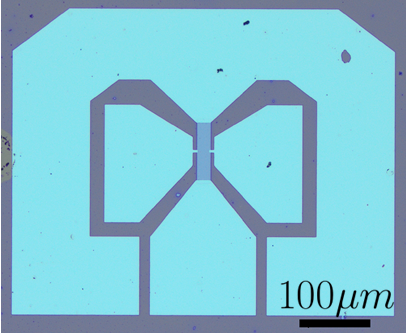
(a)

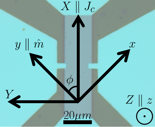
(b)

Figure 1: (a) Optical image of our Hall ST-FMR device, showing the geometry of the contact pads. This particular device featured a Pt(6)/CoFeB(6) bilayer measuring 20$\times$80 $\mu$m² (in the center, dark blue). The scale bar is 100 $\mu$m. (b) Zoomed-in optical image of the bilayer and contacts with our coordinate definitions. The $XYZ$ (capital) coordinates are fixed relative to the device geometry while $xyz$ (lowercase) coordinates are relative to the equilibrium orientation of the magnetization. The scale bar is 20 $\mu$m.

A microwave current $I_{\text{RF}}\text{Re}\left[e^{-i\omega t}\right]$ is applied, producing alternating torques with amplitudes $\tau_{x}=\tau^{0}_{\text{DL}}\cos(\phi)$ and $\tau_{z}=\tau^{0}_{z}\cos(\phi)=(\tau^{0}_{\text{FL}}+\tau^{0}_{\text{Oe}})\cos(\phi)$ in the $\hat{x}$ and $\hat{z}$ directions. With these definitions, $\tau^{0}_{\text{Oe}}$ takes a positive value by Ampere’s Law and $\tau^{0}_{\text{DL}}$ is positive for the spin Hall effect of Pt. Linearization and solution of the LLGS equation (see Supplmentary Information Sup ) allows us to calculate the oscillatory components of the magnetic moment, in complex notation,

$$\begin{split}m_{x}&=\frac{-\omega_{2}\tau_{z}+i\omega\tau_{x}}{-\gamma(B-B_{0})\omega^{+}+i\alpha\omega\omega^{+}}\\ m_{z}&=\frac{\omega_{1}\tau_{x}+i\omega\tau_{z}}{-\gamma(B-B_{0})\omega^{+}+i\alpha\omega\omega^{+}}.\end{split}$$ (4)

Here $B_{0}$ is the resonance field, $B$ is the applied external field, $\omega_{1}=\gamma B_{0}$, $\omega_{2}=\gamma(B_{0}+\mu_{0}M_{\text{eff}})$, and $\omega^{+}=\omega_{1}+\omega_{2}$; $M_{\text{eff}}$ is the in-plane saturation magnetization ($M_{S}$) minus any out-of-plane anisotropy. Note that by our definition of coordinate axes, during the precession $m_{x}=-d\phi$ and $m_{z}=-d\theta$.

Assuming that the anisotropic magnetoresistance has the form $R_{XX}=R_{0}+R_{\text{AMR}}m_{X}^{2}$, the spin-torque mixing voltage in conventional ST-FMR can be written

$$V^{\text{mix}}_{XX}=\frac{I_{\text{RF}}}{2}R_{\text{AMR}}\text{Re}\left[m_{x}\right]\sin 2\phi,$$ (5)

or

$$\ \begin{split}V^{\text{mix}}_{XX}&=\frac{I_{\text{RF}}R_{\text{AMR}}}{2\alpha\omega^{+}}\sin(2\phi)\cos(\phi)\\ &\quad\quad\quad\times\left(S(B)\tau^{0}_{\text{DL}}+A(B)\frac{\omega_{2}}{\omega}\tau^{0}_{z}\right)\end{split}$$ (6)

where we have defined the symmetric Lorentzian $S(B)=\Delta^{2}/[(B-B_{0})^{2}+\Delta^{2}]$, the antisymmetric Lorentzian $A(B)=(B-B_{0})\Delta/[(B-B_{0})^{2}+\Delta^{2}]$ and the half-width at half-maximum linewidth $\Delta=\alpha\omega/\gamma$. Here $R_{\text{AMR}}$ includes contributions from both the anisotropic magnetoresistance in the magnet and the spin Hall magnetoresistance in the Pt layer, as these produce identical contributions to the ST-FMR signals for our sample geometry (see Supplementary Information Sup ).

We can compute the transverse spin-torque mixing voltage within the same framework. We assume that the Hall resistance has the symmetry $R_{XY}=R_{\text{PHE}}m_{X}m_{Y}+R_{\text{AHE}}m_{Z}$, where $R_{\text{PHE}}$ is the scale of the planar Hall effect and $R_{\text{AHE}}$ is the scale of the anomalous Hall effect, in which case Hayashi et al. (2014)

$$V^{\text{mix}}_{XY} =\frac{I_{\text{RF}}}{2}\left(-R_{\text{PHE}}\cos 2\phi\,\text{Re}\left[m_{x}\right]+R_{\text{AHE}}\text{Re}\left[m_{z}\right]\right).$$ (7)

Using the results from Eq. (4),

$$\ \begin{split}V^{\text{mix}}_{XY}&=-\frac{I_{\text{RF}}R_{\text{PHE}}}{2\alpha\omega^{+}}\cos{(2\phi)}\cos(\phi)\\ &\quad\quad\quad\times\left(S(B)\tau^{0}_{\text{DL}}+A(B)\frac{\omega_{2}}{\omega}\tau^{0}_{z}\right)\\ &+\frac{I_{\text{RF}}R_{\text{AHE}}}{2\alpha\omega^{+}}\cos(\phi)\\ &\quad\quad\quad\times\left(S(B)\tau^{0}_{z}-A(B)\frac{\omega_{1}}{\omega}\tau^{0}_{\text{DL}}\right).\end{split}$$ (8)

The artifact signals due to spin pumping and resonant heating can also contribute to both the longitudinal and transverse ST-FMR voltages Kondou et al. (2016); Okada et al. (2019); Kumar et al. (2017). All of the artifacts we consider, SP/ISHE, LSSE/ISHE, and NE, produce resonant DC electric fields that are in-plane and perpendicular to the magnetization axis, and proportional to the square of the precession amplitude (with the precession amplitude $\propto\cos\phi$). Because these signals depend only on the precession amplitude and not phase, they have symmetric lineshapes. Taking the components in the longitudinal and transverse directions, the artifact voltages are therefore

$$\begin{split}V_{\text{art}}=E^{0}_{\text{art}}S(B)\cos^{2}\phi\begin{dcases}L\sin\phi&\text{longitudinal}\\ W\cos\phi&\text{transverse}\end{dcases}\end{split}$$ (9)

where $E^{0}_{\text{art}}=E^{0}_{\text{SP}}+E^{0}_{\text{LSSE}}+E^{0}_{\text{NE}}$ is the total electric field generated by all artifact signals. The artifact voltages for the longitudinal and transverse measurements differ only by geometric factors and angular symmetry: $L$ is the device length (parallel to the current flow) and $W$ is the transverse device width.

The electric field due to the spin pumping/inverse spin Hall effect can be calculated by the method of ref. Tserkovnyak et al. (2002a); Mosendz et al. (2010) (see Supplementary Information Sup )

$$\begin{split}E^{0}_{\text{SP}}&=\frac{e\theta_{\text{SH}}g^{\uparrow\downarrow}_{\text{eff}}}{2\pi\sum_{i}\sigma_{i}t_{i}}\lambda_{\text{sd}}\tanh\left(\frac{t_{\text{HM}}}{2\lambda_{\text{sd}}}\right)\times\\ &\left[\frac{(\tau^{0}_{\text{DL}})^{2}\omega_{1}+(\tau^{0}_{z})^{2}\omega_{2}}{\alpha^{2}\left(\omega^{+}\right)^{2}}\right].\end{split}$$ (10)

Here $\theta_{\text{SH}}$ is the spin Hall ratio in the HM (related to the damping-like spin torque efficiency by $\theta_{\text{SH}}=\xi_{\text{DL}}/T_{\text{int}}$, where $T_{\text{int}}$ is an interfacial spin transmission factor), $g^{\uparrow\downarrow}_{\text{eff}}$ is the real part of the effective spin mixing conductance, $\sigma_{i}$ ($t_{i}$) the charge conductivity (thickness) of layer $i$, and $\lambda_{\text{sd}}$ the spin diffusion length of the HM.

If one assumes that the artifacts due to resonant heating by the current-induced torques are proportional to the energy absorbed by the magnetic layer during resonant excitation, the peak DC electric field due to LSSE/ISHE and NE can be calculated similarly Holanda et al. (2017); Kikkawa et al. (2013) (see Supplementary Information Sup )

$$E^{0}_{\text{LSSE}}+E^{0}_{\text{NE}}=C\frac{M_{s}t_{\text{FM}}\alpha\omega^{+}}{2\gamma\sum_{i}\sigma_{i}t_{i}}\left[\frac{(\tau^{0}_{\text{DL}})^{2}\omega_{1}+(\tau^{0}_{z})^{2}\omega_{2}}{\alpha^{2}\left(\omega^{+}\right)^{2}}\right].$$ (11)

Here $C$ is a material-dependent prefactor. Due to the factor of $t_{\text{FM}}\alpha\omega^{+}$ in the numerator, the resonant heating contributions scale differently than the SP/ISHE as a function of FM thickness, damping, and measurement frequency.

Adding the rectification and artifact contributions [and using that $\cos^{2}\phi\sin\phi=(\sin 2\phi\cos\phi)/2$ and $\cos^{3}\phi=(\cos\phi+\cos 2\phi\cos\phi)/2$], the amplitudes of the symmetric and antisymmetric components of the total longitudinal and transverse ST-FMR signals have the angular dependence

$$\begin{split}S_{XX}(\phi)&=S_{XX}^{\text{AMR/art}}\sin 2\phi\cos\phi\\ A_{XX}(\phi)&=A_{XX}^{\text{AMR}}\sin 2\phi\cos\phi\\ S_{XY}(\phi)&=S_{XY}^{\text{PHE/art}}\cos 2\phi\cos\phi+S_{XY}^{\text{AHE/art}}\cos\phi\\ A_{XY}(\phi)&=A_{XY}^{\text{PHE}}\cos 2\phi\cos\phi+A_{XY}^{\text{AHE}}\cos\phi\end{split}$$ (12)

with the amplitude coefficients

$$\begin{split}S_{XX}^{\text{AMR/art}}&=\frac{I_{\text{RF}}}{2\alpha\omega^{+}}R_{\text{AMR}}\tau^{0}_{\text{DL}}-\frac{L}{2}E^{0}_{\text{art}}\\ &\equiv S_{XX}^{\text{AMR}}+V_{\text{art}}\\ A_{XX}^{\text{AMR}}&=\frac{I_{\text{RF}}}{2\alpha\omega^{+}}R_{\text{AMR}}\frac{\omega_{2}}{\omega}\tau^{0}_{z}\\ S_{XY}^{\text{PHE/art}}&=-\frac{I_{\text{RF}}}{2\alpha\omega^{+}}R_{\text{PHE}}\tau^{0}_{\text{DL}}-\frac{W}{2}E^{0}_{\text{art}}\\ A_{XY}^{\text{PHE}}&=-\frac{I_{\text{RF}}}{2\alpha\omega^{+}}R_{\text{PHE}}\frac{\omega_{2}}{\omega}\tau^{0}_{z}\\ S_{XY}^{\text{AHE/art}}&=\frac{I_{\text{RF}}}{2\alpha\omega^{+}}R_{\text{AHE}}\tau^{0}_{z}-\frac{W}{2}E^{0}_{\text{art}}\\ A_{XY}^{\text{AHE}}&=-\frac{I_{\text{RF}}}{2\alpha\omega^{+}}R_{\text{AHE}}\frac{\omega_{1}}{\omega}\tau^{0}_{\text{DL}}.\end{split}$$ (13)

One can see that all of the $S_{XX}$ and $S_{XY}$ rectification signals are contaminated by artifact voltages. If one measures just $S_{XX}$ and $A_{XX}$ for in-plane magnetic fields (as in conventional ST-FMR) there is no way to distinguish $\tau^{0}_{\text{DL}}$ from the artifact contributions. However, $\tau^{0}_{\text{DL}}$ appears by itself, without any artifact contamination, in the coefficient $A_{XY}^{\text{AHE}}$. One way to achieve a measurement of $\tau^{0}_{\text{DL}}$, free of these artifacts, is therefore to directly use the expression for $A_{XY}^{\text{AHE}}$ in Eq. (13) along with careful calibration of $I_{\text{RF}}$, $\alpha$, and $R_{\text{AHE}}$. The out-of-plane torque $\tau^{0}_{z}$ can similarly be determined from $A_{XX}^{\text{AMR}}$ or $A_{XY}^{\text{PHE}}$. Alternatively, the expressions in Eq. (13) also allow $E^{0}_{\text{art}}$ and the torque efficiencies $\xi_{\text{DL}}$ and $\xi_{\text{FL}}$ to be measured without calibrating $I_{\text{RF}}$, $\alpha$, and the the magnetoresistance scales by taking appropriate ratios to cancel prefactors. We can do so using measurements of either the set of parameters $\{S_{XX}^{\text{AMR/art}},A_{XX}^{\text{AMR}},S_{XY}^{\text{AHE/art}},A_{XY}^{\text{AHE}}\}$ or $\{S_{XY}^{\text{PHE/art}},A_{XY}^{\text{PHE}},S_{XY}^{\text{AHE/art}},A_{XY}^{\text{AHE}}\}$. We do not expect that the equations involving $R_{\text{AMR}}$ and $R_{\text{PHE}}$ are physically independent because anisotropic magnetoresistance and the planar Hall effect originate from the same microscopic mechanism. Therefore if the assumptions of our model are correct these two strategies for taking ratios to cancel prefactors must agree modulo experimental noise. We will perform both calculations, and test their agreement as a consistency check.

First, using that on resonance $\omega=\sqrt{\omega_{1}\omega_{2}}$ we calculate the ratio $\eta\equiv(\tau^{0}_{\text{DL}}/\tau^{0}_{z})\sqrt{\omega_{1}/\omega_{2}}$ employing the pair of parameters $S$ and $A$ associated with each of the AMR, PHE, and AHE:

$$\eta=\frac{-A^{\text{AHE}}_{XY}}{S^{\text{AHE/art}}_{XY}+W(E_{\text{art}}/2)}=\\$$

$$[left=\empheqlbrace] \frac{S^{\text{PHE/art}}_{XY}+W(E_{\text{art}}/2)}{A^{\text{PHE}}_{XY}}$$ (14a)

$$\frac{S^{\text{AMR/art}}_{XX}+L(E_{\text{art}}/2)}{A^{\text{AMR}}_{XX}}$$ (14b)

Using the measured amplitude coefficients, one can solve separately for $E_{\text{art}}$ using either Eq. (14a) or (14b), and check consistency.

It still remains to determine $\tau^{0}_{\text{DL}}$ and to separate the two contributions to $\tau^{0}_{z}=\tau^{0}_{\text{FL}}+\tau^{0}_{\text{Oe}}$. We choose to do this using a method from ref. Pai et al. (2015), in a way that determines both the of the spin-torque efficiencies $\xi_{\text{DL}}$ and $\xi_{\text{FL}}$ at the same time without requiring a separate calibration of $I_{\text{RF}}$. We perform measurements for a series of samples with different thicknesses of the ferromagnetic layer and determine $\eta=(\tau^{0}_{\text{DL}}/\tau^{0}_{z})\sqrt{\omega_{1}/\omega_{2}}$ for each sample from any of the expressions in Eqs. (14a,14b), after solving for $E_{\text{art}}$. We then define

$$\xi_{\text{FMR}} \equiv\eta\frac{e\mu_{0}M_{s}t_{\text{HM}}t_{\text{FM}}}{\hbar}\sqrt{1+\frac{\mu_{0}M_{\text{eff}}}{B_{0}}}$$ (15)

so that using Equations (2) & (3), and that by Ampere’s Law $\tau^{0}_{\text{Oe}}=\gamma\mu_{0}J_{e}t_{\text{HM}}/2$ one has

$$\frac{1}{\xi_{\text{FMR}}} =\frac{1}{\xi_{\text{DL}}}\left(1+\frac{\hbar}{e}\frac{\xi_{\text{FL}}}{\mu_{0}M_{s}t_{\text{FM}}t_{\text{HM}}}\right).$$ (16)

Performing a linear fit of $1/\xi_{\text{FMR}}$ vs. $1/t_{\text{FM}}$ then can be used to determine $1/\xi_{\text{DL}}$ (from the intercept) and $\xi_{\text{FL}}$ (from the slope).

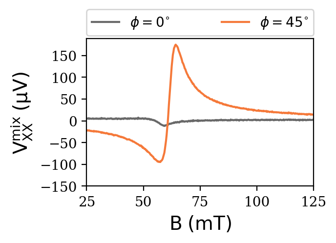
(a)

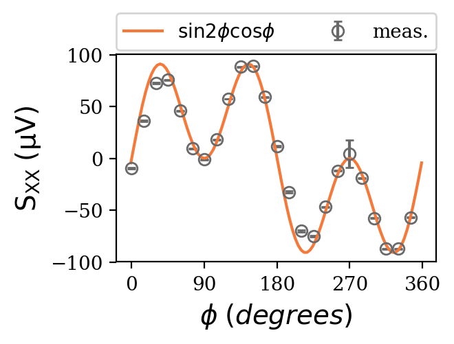
(b)

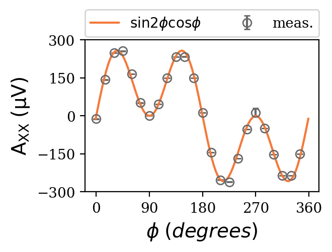
(c)

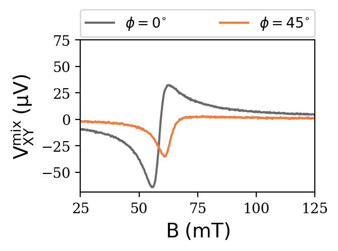
(d)

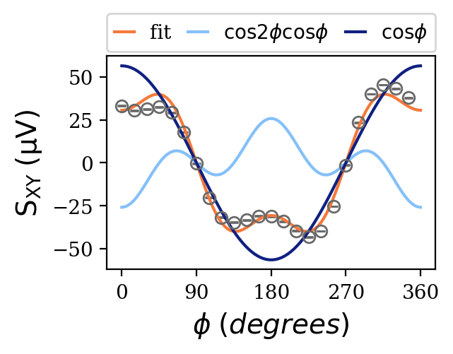
(e)

(f)

Figure 2: ST-FMR measurements of a Pt(6 nm)/CoFeB(6 nm) sample for a measurement frequency $f=8$ GHz. (a) Longitudinal resonant signals for field sweeps with two different field angles. (b) & (c) Symmetric ($S_{XX}$) and antisymmetric ($A_{XX}$) Lorentzian fit components for the longitudinal resonant signal as a function of the external field angle. (d) Transverse resonant signals for field sweeps with two different field angles. (e) & (f) Symmetric ($S_{XY}$) and antisymmetric ($A_{XY}$) Lorentzian fit components for the transverse resonant signal as a function of the external field angle. The orange fit line in (b) & (c) is a fit to $\sin 2\phi\cos\phi$ (AMR); the light and dark blue fit lines in (e,f) are fits to $\cos 2\phi\cos\phi$ (PHE) and $\cos\phi$ (AHE), respectively, and their sum (orange) fits the data.

IV Measurements

We used DC-magnetron sputtering to grow multiayers with the structure substrate/Ta(1)/Pt(6)/ferromagnet($t_{\text{FM}}$)/Al(1) (where numbers in parentheses are thicknesses in nm), using three different ferromagnets (FMs): Co₄₀Fe₄₀B₂₀ (CoFeB), permalloy (Ni₈₁Fe₁₉ = Py) and Co₉₀Fe₁₀ (CoFe). Each of the three FMs is expected to have different AMR, PHE, and AHE values, and therefore different strengths of rectified spin-torque signals relative to the artifacts. In particular, CoFeB has weak planar magnetoresistances (AMR and PHE), and has been argued previously to exhibit a significant contribution from SP/ISHE in ST-FMR Kondou et al. (2016); Okada et al. (2019). The CoFeB devices were grown with $t_{\text{FM}}=\{2,3,4,6,8,10\}$ in separate depositions. The Py and Co₉₀Fe₁₀ devices were grown with single relatively-large thicknesses to give measurable artifact signals: $t_{\text{Py}}$= 8 nm and $t_{\text{CoFe}}$= 6 nm. All devices were grown on high-resistivity ($>2\times 10^{4}\,\Omega\text{-cm}$), thermally-oxidized silicon wafers to prevent RF current leakage or capacitive coupling. The Ta was used as a seed layer and has negligible contribution to the SOTs we measure due to the low conductivity of Ta relative to Pt ($\rho_{\text{Pt}}$ = 20.4 $\mu\Omega$cm, $\rho_{\text{CoFeB}}$ = 110 $\mu\Omega$cm). The Al cap layer protects the layers below it, and is oxidized upon exposure to atmosphere.

The as-deposited samples were patterned using photolithography and Ar ion-milling to define rectangular bars ranging in size from 20 $\times$ 40 $\mu$m to 40 $\times$ 80 $\mu$m with various aspect ratios. The transverse leads and contact pads were then made using a second photolithography step, deposited by sputtering Ti(3 nm)/Pt(75 nm) and formed by lift-off so that the side channels extended a few microns on top of the main bar (see Fig. 1). We were careful that the magnetic layer did not extend beyond the defined rectangle into the transverse leads. In early devices, we etched full Hall-bar shapes within the first layer of lithography so that the transverse leads included some of the same magnetic layer as the main channel. For those early devices, we found that the resulting analyses of spin-orbit torques produced anomalous results, varying with the dimensions of the leads and the contact separation. This could possibly be due to spatial non-uniformities in the magnetic orientation and precession, as was speculated in Bose et al. (2017). Ultimately, the magnetic bilayer was left to be simply rectangular to promote uniform precession modes, and this removed the anomalous geometry dependence.

For the ST-FMR measurements, we connected the devices to an amplitude-modulated (“AM” with $f_{\text{AM}}\approx$ 1700 Hz) microwave source through the AC port of a bias tee and to a lock-in amplifier through the DC port, which detected the longitudinal signal. Another lock-in amplifier measured the DC voltage across the Hall leads of the device. Both lock-in amplifiers referenced the same AM signal, and we collected ST-FMR data in both the longitudinal and transverse directions simultaneously. An in-plane applied magnetic field was applied at varying angles $\phi$ using a projected-field magnet. We used fixed microwave frequencies in the range 7-12 GHz, applied 20 dBm of microwave power, and all measurements were performed at room temperature. In Figs. 2(a) and 2(d) we show examples of the detected resonant signals from the parallel ($XX$) and transverse ($XY$) lock-ins for the Pt(6)/CoFeB(6) sample.

Both the longitudinal and transverse resonances are well-fit to a sum of symmetric and antisymmetric Lorentzian peaks, with varying relative weights. For each sample we performed field-swept measurements at a variety of angles $\phi$, extracting the symmetric and antisymmetric components of the resonances for both the longitudinal and transverse signals. The results for a Pt(6)/CoFeB(6) sample are shown in Fig. 2(b,c,e,f), along with fits to Eq. (12). Analogous results for Pt(6)/Py(8) and Pt(6)/CoFe(6) samples are shown in the Supplementary Information Sup .

We find excellent agreement with the expected angular dependences for $S_{\text{XX}}$, $A_{\text{XX}}$, and $A_{\text{XY}}$. For $S_{\text{XY}}$ the dominant contributions to the angular dependence are, as expected the $\cos 2\phi\cos\phi$ and $\cos\phi$ terms, but in addition, we detect a small component approximately proportional to $\sin 2\phi$. This additional contribution is less than 10% of the larger terms in $S_{\text{XY}}$ for all thicknesses of CoFeB, small enough that it is not included in the fit shown in Fig. 2(e). It is more significant in the CoFe and Py samples that we measured, though still smaller than the $\cos 2\phi\cos\phi$ and $\cos\phi$ amplitudes in $S_{\text{XY}}$ (see Supplementary Information Sup ). A $\sin 2\phi$ contribution can only arise from a breaking of mirror symmetry relative to the sample’s $\hat{Y}$-$\hat{Z}$ plane (see Supplementary Information Sup ). This symmetry is broken in our samples by the different contact geometries on the two ends of the sample wire (see Fig. 1(a)). The form of the $\sin 2\phi$ signal can be explained as due resonant heating that produces an in-plane thermal gradient in the longitudinal direction of the sample (due e.g. to differences in heat sinking at the two ends) that is transduced to a tranverse voltage with the symmetry of the planar Hall effect ($\propto m_{X}m_{Y}$). We have checked that the signal is not due to a sample tilt or to a non-resonant DC current that might arise from rectification of the applied microwave signal at the sample contacts. All of the other Fourier components that are the main subject of our analysis maintain the $\hat{Y}$-$\hat{Z}$-plane mirror symmetry, and so they cannot be altered at first order by a process that breaks this symmetry. Being a separate Fourier component, the $\sin 2\phi$ contribution also does not affect the fits to Eq. (12) to determine the six amplitude coefficients $S_{XX}^{\text{AMR/art}}$, $A_{XX}^{\text{AMR}}$, $S_{XY}^{\text{PHE/art}}$, $A_{XY}^{\text{PHE}}$, $S_{XY}^{\text{AHE/art}}$, and $A_{XY}^{\text{AHE}}$. Using these coefficients, we calculate $E_{\text{art}}$ by solving Eqs. (14a) or (14b). There is a potential ambiguity in which roots of Eqs. (14a) and (14b) to select when applying the quadratic formula. In our measurements, one root would give unphysical results, e.g. a sign change of $\xi_{\text{DL}}$. An important check of our method (and a check that the $\sin 2\phi$ term in $S_{XY}$ does not contaminate the analysis) is that these two independent methods for determining $E^{0}_{\text{art}}$ (Eqs. (14a) and (14b)) give consistent results. We show below that this is indeed the case.

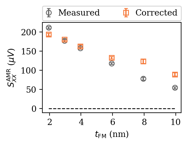
(a)

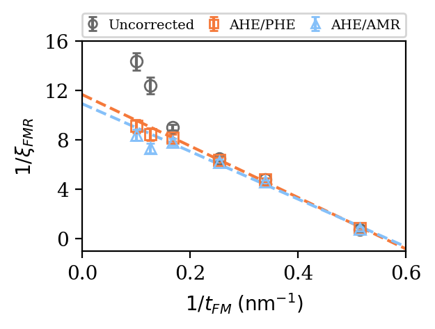
(b)

Figure 3: (a) The uncorrected measured value of $S_{XX}^{\text{AMR}}$ vs. $t_{\text{FM}}$, together with the value corrected by removing the artifact voltage. (b) The inverse $\xi_{\text{FMR}}$ vs. inverse $t_{\text{FM}}$. The y-intercept of the line is $1/\xi_{\text{DL}}$ and the slope is proportional to $\xi_{\text{FL}}$ as in Eq. (16). The two fit lines are color-matched fits to the data points from the AHE/PHE and AHE/AMR corrections.

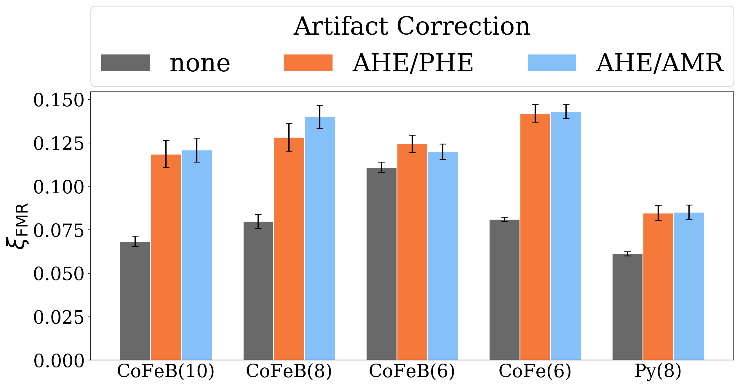
Figure 4: $\xi_{\text{FMR}}$ for various device stacks. The gray (left) bars show values without correction for the artifacts, and the orange and blue (center, right) bars show values corrected using the determination of the artifact voltages using Eqs. (14a) and (14b), respectively.

Figure 3(a) shows the total amplitude of the longitudinal symmetric ST-FMR component (labeled as “Measured”), and the corrected value $S^{\text{AMR}}_{\text{XX}}$ from which $V_{\text{art}}$ has been subtracted. For CoFeB layer thicknesses 6 nm and below, the magnitude of $V_{\text{art}}$ is much less than the magnitude of $S^{\text{AMR}}_{\text{XX}}$, so that the artifacts have little effect on ST-FMR measurements of the spin-orbit torques. However, with increasing CoFeB thickness the magnitude of $S^{\text{AMR}}_{\text{XX}}$ decreases and $V_{\text{art}}$ grows, so we find experimentally that for the CoFeB layers thicker than 6 nm the artifact voltage becomes a significant fraction of the total signal. In this regime, $V_{\text{art}}$ and $S^{\text{AMR}}_{\text{XX}}$ contribute to $S_{\text{XX}}(\phi)$ with opposite signs Schreier et al. (2014), with the consequence that if the artifact contributions are neglected in the conventional ST-FMR analysis, the result is an underestimate of the strength of $\tau^{0}_{\text{DL}}$. In this respect our results conflict with some conclusions Kondou et al. (2016); Okada et al. (2019) that neglecting the SP/ISHE contribution produces an overestimate of $\tau^{0}_{\text{DL}}$.

Analysis of the dependence of $1/\xi_{\text{FMR}}$ as a function of $1/t_{\text{FM}}$ allows a determination of the underlying spin-torque efficiencies $\xi_{\text{DL}}$ and $\xi_{\text{FL}}$ using Eq. (16). The results for the CoFeB series of samples is shown in Fig. 3(b). If one does not correct for the contribution of the artifacts, the calculated values of $1/\xi_{\text{FMR}}$ depart upward from the expected linear dependence for $t_{\text{FM}}\gtrsim 6$ nm. Similar results have been reported previously in Pai et al. (2015) where the non-linearity was speculated to be from SP/ISHE, and the spin-torque efficiencies were determined by fitting only to the thinner FM stacks. After we correct for the artifact contribution, we find good agreement with the expected linear dependence over the full thickness range. From the linear fit, we determine $\xi_{\text{DL}}=$ 0.090(6) and $\xi_{\text{FL}}=$ -0.020(2).

For the Pt(6 nm)/Py(8 nm) and Pt(6 nm)/CoFe(6 nm) samples we find the same configuration of signs as for the thicker Pt/CoFeB samples: $V_{\text{art}}$ partially cancels $S^{\text{AMR}}_{\text{XX}}$ so that the true mixing signal is larger than the measured amplitude of $S_{\text{XX}}(\phi)$. The results of the calculation of $\xi_{\text{FMR}}$ according to Eq. (15) are shown in Fig. 4 for five selected samples, both without and with the correction for artifacts. In determining $\xi_{\text{FMR}}$ we use values for $M_{s}$ determined by room temperature vibrating sample magnetometry (VSM) and values for $\mu_{0}M_{\text{eff}}$ determined by fits of the ST-FMR resonant fields as a function of frequency. These values are: for CoFeB $M_{s}=9.8\times 10^{5}$ A/m, $\mu_{0}M_{\text{eff}}=$ 0.6 – 1.4 T (depending on thickness); for Py $M_{s}=7.5\times 10^{5}$ A/m, $\mu_{0}M_{\text{eff}}=1.01$ T; and for CoFe $M_{s}=9.1\times 10^{5}$ A/m, $\mu_{0}M_{\text{eff}}=1.66$ T. If a magnetic dead layer was observed in VSM, the dead layer thickness was subtracted from $t_{\text{FM}}$. In all cases shown in Fig. 4, we find that correcting for the artifact contribution increases our estimates for the values of $\xi_{\text{FMR}}$. The value of $\xi_{\text{FMR}}$ is smaller for the Pt/Py sample than for Pt/CoFeB or Pt/CoFe primarily because $\xi_{\text{FL}}$ is both small and has a positive sign for Pt/Py Fan et al. (2013); Nan et al. (2015).

The dependence of the artifact voltage, $V_{\text{art}}$, on the ferromagnetic layer thickness is shown in Fig. 5 for the longitudinal ST-FMR component of the Pt/CoFeB series of samples. The data are compared to an estimate of the SP/ISHE contribution from Eq. (10), using the parameters (appropriate for the resistivity of our Pt layers, $\rho_{\text{Pt}}=20.4$ $\mu\Omega$cm): $\theta_{\text{SH}}=0.32$ Zhu et al. (2019b); Pai et al. (2015), $g^{\uparrow\downarrow}_{\text{eff}}=8.26\times 10^{18}$ m^-2 Zhu et al. (2019b), and $\lambda_{\text{sd}}=3.7$ nm Nguyen et al. (2016). The other quantities in Eq. (10) were measured for our samples, including the variation as a function of CoFeB thickness. The comparison therefore includes no adjustable fitting parameters, but given that there is considerable disagreement in the literature about the values of the parameters $\theta_{\text{SH}}$, $g^{\uparrow\downarrow}_{\text{eff}}$, and $\lambda_{\text{sd}}$, one should still be careful about drawing quantitative conclusions. The comparison indicates to us that for the samples with $t_{\text{FM}}\geq$ 3 nm the SP/ISHE theory predicts the correct sign and can roughly capture the overall magnitude and thickness-dependence of the measured artifact signal. However, the measured artifact voltage for $t_{\text{FM}}$= 2 nm has the opposite sign, inconsistent with the SP/ISHE. We are confident that the measured sign change is real, because we have measured and performed the analysis on five Pt(6 nm)/CoFeB(2 nm) devices with varied geometries, with consistent results.

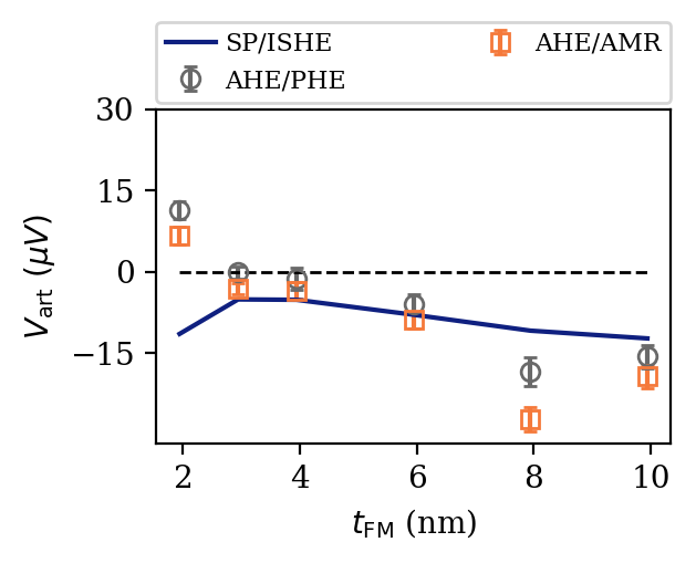
Figure 5: The artifact voltage as a function of the FM thickness in Pt(6 nm)/CoFeB samples. The two types of data points reflect the two correction equations ((14a) and (14b)). The line is the estimated SP/ISHE contribution, determined using the parameters described in the text, with no adjustable parameters.

Given that the SP/ISHE cannot explain the sign change in the artifact voltage for our $t_{\text{FM}}$= 2 nm samples, we suggest that resonant heating effects might be comparable to the SP/ISHE in our Pt(6 nm)/CoFeB samples, with sufficient strength to reverse the overall sign of the artifact voltage for our thinnest samples. This suggestion differs from previous studies on Pt/YIG samples, for which frequency-dependent measurements demonstrated that SP/ISHE signals dominate over resonant heating artifacts Iguchi and Saitoh (2017); Iguchi et al. (2012). However, the relative strength of the heating effects and SP/ISHE should scale proportional to the damping $\alpha$ (compare Eqs. (10) and (11)), so that the heating effects should be more significant in higher-damping ferromagnetic metals compared to lower-damping YIG. We calculate that the resonant heating due to the excitation of magnetic precession for our 2 nm samples is $\sim 2.5\times 10^{4}$ Wm^-2 (Supplementary Information Sup ), only about a factor of 5 less than the Ohmic heating per unit area in the CoFeB, $\sim 1.2\times 10^{5}$ Wm^-2. We suggest that this is sufficient to measurably alter the thermal gradients within the sample at resonance and induce resonant signals from the LSSE and/or Nernst effects. Due to an increase in the damping coefficient $\alpha$ with decreasing magnetic thickness, the ratio of the resonant heating to Ohmic heating is significantly greater for the 2 nm CoFeB samples than for the thicker magnetic layers (see Supplmentary Information Sup ).

As noted in the introduction, past experiments have shown a discrepancy between measurements of $\xi_{\text{DL}}$ using low frequency second harmonic Hall and ST-FMR techniques. To see if our correction for the artifact voltages in ST-FMR alleviates the discrepancy between the two techniques, we carried out low frequency second harmonic Hall measurements on the same Pt/CoFeB bilayers Sup . We found that the low frequency second harmonic measurements of $\xi_{\text{DL}}$ were still approximately 60% larger than what we measured by ST-FMR, even after correcting ST-FMR for spin pumping and resonant heating. This persisting quantitative difference suggests that the assumptions used in analyzing one or both of these experiments are missing an important bit of physics. Our analysis indicates that this missing physics is not simply the neglect of spin pumping or a simple heating-induced voltage in the ST-FMR results, and therefore more work must be done to understand the source of the disagreement.

V Conclusion

In conclusion, we have demonstrated that the rectification signal used to measure the strength of spin-orbit torques in spin-torque ferromagnetic resonance (ST-FMR) can be separated from artifact voltages that may arise due to spin pumping and resonant heating by performing ST-FMR in the transverse (Hall) configuration as well as the usual longitudinal configuration. For Pt(6 nm)/CoFeB($t_{\text{FM}}$) samples, the artifact voltages are small compared to the rectification signal for $t_{\text{FM}}<$ 6 nm, but they can become a significant part of the measured signal for thicker magnetic layers. The sign and overall magnitude of the measured artifact voltage for these thicker layers are consistent with expectations for the SP/ISHE effect signal. However, the sign of the artifact voltage is reversed for our thinnest magnetic layers, with $t_{\text{FM}}$ = 2 nm. This sign reversal cannot be explained by the SP/ISHE, so we suggest that it may be caused by a resonant heating effect.

VI Acknowledgements

This research was supported in part by task 2776.047 in ASCENT, one of six centers in JUMP, a Semiconductor Research Corporation program sponsored by DARPA, and in part by the National Science Foundation (DMR-1708499). The devices were fabricated using the shared facilities of the Cornell NanoScale Facility, a member of the National Nanotechnology Coordinated Infrastructure (NNCI), and the Cornell Center for Materials Research, both of which are supported by the NSF (NNCI-1542081 and DMR-1719875).

See pages 1 of ./supporting/SuppSee pages 2 of ./supporting/SuppSee pages 3 of ./supporting/SuppSee pages 4 of ./supporting/SuppSee pages 5 of ./supporting/SuppSee pages 6 of ./supporting/SuppSee pages 7 of ./supporting/SuppSee pages 8 of ./supporting/SuppSee pages 9 of ./supporting/SuppSee pages 10 of ./supporting/SuppSee pages 11 of ./supporting/SuppSee pages 12 of ./supporting/SuppSee pages 13 of ./supporting/SuppSee pages 14 of ./supporting/SuppSee pages 15 of ./supporting/Supp

References

- Brataas et al. (2012) A. Brataas, A. D Kent, and H. Ohno, Nature Materials 11, 372 (2012).
- Wang et al. (2013) K. L. Wang, J. G. Alzate, and P. K. Amiri, Journal of Physics D: Applied Physics 46, 074003 (2013).
- Oboril et al. (2015) F. Oboril, R. Bishnoi, M. Ebrahimi, and M. B. Tahoori, IEEE Transactions on Computer-Aided Design of Integrated Circuits and Systems 34, 367 (2015).
- Liu et al. (2011) L. Liu, T. Moriyama, D. C. Ralph, and R. A. Buhrman, Phys. Rev. Lett. 106, 036601 (2011).
- Liu et al. (2012) L. Liu, C.-F. Pai, Y. Li, H. W. Tseng, D. C. Ralph, and R. A. Buhrman, Science 336, 555 (2012).
- Mellnik et al. (2014) A. R. Mellnik, J. S. Lee, A. Richardella, J. L. Grab, P. J. Mintun, M. H. Fischer, A. Vaezi, A. Manchon, E.-A. Kim, N. Samarth, and D. C. Ralph, Nature 511, 449 (2014).
- Pi et al. (2010) U. H. Pi, K. Won Kim, J. Y. Bae, S. C. Lee, Y. J. Cho, K. S. Kim, and S. Seo, Applied Physics Letters 97, 162507 (2010).
- Garello et al. (2013) K. Garello, I. M. Miron, C. O. Avci, F. Freimuth, Y. Mokrousov, S. Blügel, S. Auffret, O. Boulle, G. Gaudin, and P. Gambardella, Nature Nanotechnology 8, 587 (2013).
- Hayashi et al. (2014) M. Hayashi, J. Kim, M. Yamanouchi, and H. Ohno, Phys. Rev. B 89, 144425 (2014).
- Fan et al. (2014) X. Fan, H. Celik, J. Wu, C. Ni, K.-J. Lee, V. O. Lorenz, and J. Q. Xiao, Nature Communications 5, 3042 (2014).
- Fan et al. (2016) X. Fan, A. R. Mellnik, W. Wang, N. Reynolds, T. Wang, H. Celik, V. O. Lorenz, D. C. Ralph, and J. Q. Xiao, Applied Physics Letters 109, 122406 (2016).
- Sun (2000) J. Z. Sun, Physical Review B 62, 570 (2000).
- Althammer et al. (2013) M. Althammer, S. Meyer, H. Nakayama, M. Schreier, S. Altmannshofer, M. Weiler, H. Huebl, S. Geprägs, M. Opel, R. Gross, D. Meier, C. Klewe, T. Kuschel, J.-M. Schmalhorst, G. Reiss, L. Shen, A. Gupta, Y.-T. Chen, G. E. W. Bauer, E. Saitoh, and S. T. B. Goennenwein, Phys. Rev. B 87, 224401 (2013).
- Kim et al. (2016) J. Kim, P. Sheng, S. Takahashi, S. Mitani, and M. Hayashi, Phys. Rev. Lett. 116, 097201 (2016).
- Emori et al. (2014) S. Emori, E. Martinez, K.-J. Lee, H.-W. Lee, U. Bauer, S.-M. Ahn, P. Agrawal, D. C. Bono, and G. S. D. Beach, Phys. Rev. B 90, 184427 (2014).
- Pai et al. (2016) C.-F. Pai, M. Mann, A. J. Tan, and G. S. D. Beach, Phys. Rev. B 93, 144409 (2016).
- Pai et al. (2015) C.-F. Pai, Y. Ou, L. H. Vilela-Leão, D. C. Ralph, and R. A. Buhrman, Phys. Rev. B 92, 064426 (2015).
- Tao et al. (2018) X. Tao, Q. Liu, B. Miao, R. Yu, Z. Feng, L. Sun, B. You, J. Du, K. Chen, S. Zhang, L. Zhang, Z. Yuan, D. Wu, and H. Ding, Science Advances 4, 1670 (2018).
- Zhu et al. (2019a) L. Zhu, K. Sobotkiewich, X. Ma, X. Li, D. C. Ralph, and R. A. Buhrman, Advanced Functional Materials 29, 1805822 (2019a).
- Lau and Hayashi (2017) Y.-C. Lau and M. Hayashi, Japanese Journal of Applied Physics 56, 0802B5 (2017).
- Tserkovnyak et al. (2002a) Y. Tserkovnyak, A. Brataas, and G. E. W. Bauer, Phys. Rev. Lett. 88, 117601 (2002a).
- Tserkovnyak et al. (2002b) Y. Tserkovnyak, A. Brataas, and G. E. W. Bauer, Phys. Rev. B 66, 224403 (2002b).
- Mosendz et al. (2010) O. Mosendz, V. Vlaminck, J. E. Pearson, F. Y. Fradin, G. E. W. Bauer, S. D. Bader, and A. Hoffmann, Phys. Rev. B 82, 214403 (2010).
- Azevedo et al. (2011) A. Azevedo, L. H. Vilela-Leão, R. L. Rodríguez-Suárez, A. F. Lacerda Santos, and S. M. Rezende, Phys. Rev. B 83, 144402 (2011).
- Uchida et al. (2010) K.-i. Uchida, H. Adachi, T. Ota, H. Nakayama, S. Maekawa, and E. Saitoh, Applied Physics Letters 97, 172505 (2010).
- Holanda et al. (2017) J. Holanda, O. Alves Santos, R. L. Rodríguez-Suárez, A. Azevedo, and S. M. Rezende, Phys. Rev. B 95, 134432 (2017).
- Lee et al. (2015) K.-D. Lee, D.-J. Kim, H. Yeon Lee, S.-H. Kim, J.-H. Lee, K.-M. Lee, J.-R. Jeong, K.-S. Lee, H.-S. Song, J.-W. Sohn, S.-C. Shin, and B.-G. Park, Scientific Reports 5, 10249 (2015).
- Kikkawa et al. (2013) T. Kikkawa, K. Uchida, Y. Shiomi, Z. Qiu, D. Hou, D. Tian, H. Nakayama, X.-F. Jin, and E. Saitoh, Phys. Rev. Lett. 110, 067207 (2013).
- Avci et al. (2014) C. O. Avci, K. Garello, M. Gabureac, A. Ghosh, A. Fuhrer, S. F. Alvarado, and P. Gambardella, Phys. Rev. B 90, 224427 (2014).
- Roschewsky et al. (2019) N. Roschewsky, E. S. Walker, P. Gowtham, S. Muschinske, F. Hellman, S. R. Bank, and S. Salahuddin, Phys. Rev. B 99, 195103 (2019).
- Kondou et al. (2016) K. Kondou, H. Sukegawa, S. Kasai, S. Mitani, Y. Niimi, and Y. Otani, Applied Physics Express 9, 023002 (2016).
- Okada et al. (2019) A. Okada, Y. Takeuchi, K. Furuya, C. Zhang, H. Sato, S. Fukami, and H. Ohno, Phys. Rev. Applied 12, 014040 (2019).
- Kumar et al. (2017) A. Kumar, S. Akansel, H. Stopfel, M. Fazlali, J. Åkerman, R. Brucas, and P. Svedlindh, Phys. Rev. B 95, 064406 (2017).
- Tulapurkar et al. (2005) A. Tulapurkar, Y. Suzuki, A. Fukushima, H. Kubota, H. Maehara, K. Tsunekawa, D. Djayaprawira, N. Watanabe, and S. Yuasa, Nature 438, 339 (2005).
- Sankey et al. (2006) J. C. Sankey, P. M. Braganca, A. G. F. Garcia, I. N. Krivorotov, R. A. Buhrman, and D. C. Ralph, Phys. Rev. Lett. 96, 227601 (2006).
- Lustikova et al. (2015) J. Lustikova, Y. Shiomi, and E. Saitoh, Phys. Rev. B 92, 224436 (2015).
- Jungfleisch et al. (2015) M. B. Jungfleisch, A. V. Chumak, A. Kehlberger, V. Lauer, D. H. Kim, M. C. Onbasli, C. A. Ross, M. Kläui, and B. Hillebrands, Phys. Rev. B 91, 134407 (2015).
- Nakayama et al. (2012) H. Nakayama, K. Ando, K. Harii, T. Yoshino, R. Takahashi, Y. Kajiwara, K. Uchida, Y. Fujikawa, and E. Saitoh, Phys. Rev. B 85, 144408 (2012).
- Rezende et al. (2014) S. M. Rezende, R. L. Rodríguez-Suárez, R. O. Cunha, A. R. Rodrigues, F. L. A. Machado, G. A. Fonseca Guerra, J. C. Lopez Ortiz, and A. Azevedo, Phys. Rev. B 89, 014416 (2014).
- Saitoh et al. (2006) E. Saitoh, M. Ueda, H. Miyajima, and G. Tatara, Applied Physics Letters 88, 182509 (2006).
- Iguchi and Saitoh (2017) R. Iguchi and E. Saitoh, Journal of the Physical Society of Japan 86, 011003 (2017).
- Bose et al. (2017) A. Bose, S. Dutta, S. Bhuktare, H. Singh, and A. A. Tulapurkar, Applied Physics Letters 111, 162405 (2017).
- Keller et al. (2017) S. Keller, J. Greser, M. R. Schweizer, A. Conca, V. Lauer, C. Dubs, B. Hillebrands, and E. T. Papaioannou, Physical Review B 96 (2017), 10.1103/physrevb.96.024437.
- Harder et al. (2016) M. Harder, Y. Gui, and C.-M. Hu, Physics Reports 661, 1 (2016), electrical detection of magnetization dynamics via spin rectification effects.
- (45) Supplemental Materials: Transverse and Longitudinal Spin-Torque Ferromagnetic Resonance for Improved Measurements of Spin-Orbit Torques .
- Schreier et al. (2014) M. Schreier, G. E. W. Bauer, V. I. Vasyuchka, J. Flipse, K. ichi Uchida, J. Lotze, V. Lauer, A. V. Chumak, A. A. Serga, S. Daimon, T. Kikkawa, E. Saitoh, B. J. van Wees, B. Hillebrands, R. Gross, and S. T. B. Goennenwein, Journal of Physics D: Applied Physics 48, 025001 (2014).
- Fan et al. (2013) X. Fan, J. Wu, Y. Chen, M. J. Jerry, H. Zhang, and J. Q. Xiao, Nature Communications 4, 1799 (2013).
- Nan et al. (2015) T. Nan, S. Emori, C. T. Boone, X. Wang, T. M. Oxholm, J. G. Jones, B. M. Howe, G. J. Brown, and N. X. Sun, Phys. Rev. B 91, 214416 (2015).
- Zhu et al. (2019b) L. Zhu, D. C. Ralph, and R. A. Buhrman, Phys. Rev. Lett. 123, 057203 (2019b).
- Nguyen et al. (2016) M.-H. Nguyen, D. C. Ralph, and R. A. Buhrman, Phys. Rev. Lett. 116, 126601 (2016).
- Iguchi et al. (2012) R. Iguchi, K. Ando, R. Takahashi, T. An, E. Saitoh, and T. Sato, Japanese Journal of Applied Physics 51, 103004 (2012).