Faster Graph Embeddings via Coarsening

Abstract

Graph embeddings are a ubiquitous tool for machine learning tasks, such as node classification and link prediction, on graph-structured data. However, computing the embeddings for large-scale graphs is prohibitively inefficient even if we are interested only in a small subset of relevant vertices. To address this, we present an efficient graph coarsening approach, based on Schur complements, for computing the embedding of the relevant vertices. We prove that these embeddings are preserved exactly by the Schur complement graph that is obtained via Gaussian elimination on the non-relevant vertices. As computing Schur complements is expensive, we give a nearly-linear time algorithm that generates a coarsened graph on the relevant vertices that provably matches the Schur complement in expectation in each iteration. Our experiments involving prediction tasks on graphs demonstrate that computing embeddings on the coarsened graph, rather than the entire graph, leads to significant time savings without sacrificing accuracy.

1 Introduction

Over the past several years, network embeddings have been demonstrated to be a remarkably powerful tool for learning unsupervised representations for nodes in a network (Perozzi et al.,, 2014; Tang et al.,, 2015; Grover and Leskovec,, 2016). Broadly speaking, the objective is to learn a low-dimensional vector for each node that captures the structure of its neighborhood. These embeddings have proved to be very effective for downstream machine learning tasks in networks such as node classification and link prediction (Tang et al.,, 2015; Hamilton et al.,, 2017).

While some of these graph embedding approaches are explicitly based on matrix-factorization (Tang and Liu,, 2011; Bruna et al.,, 2014; Cao et al.,, 2015), some of the other popular methods, such as DeepWalk (Perozzi et al.,, 2014) and LINE (Tang et al.,, 2015), can be viewed as approximately factoring random walk matrices constructed from the graph. A new approach proposed by Qiu et al., (2018) called NetMF explicitly computes a low-rank approximation of random-walk matrices using a Singular Value Decomposition (SVD), and significantly outperforms the DeepWalk and LINE embeddings for benchmark network-mining tasks.

Despite the performance gains, explicit matrix factorization results in poor scaling performance. The matrix factorization-based approaches typically require computing the singular value decomposition (SVD) of an $n\times n$ matrix, where $n$ is the number of vertices in the graph. In cases where this matrix is constructed by taking several steps of random walks, e.g., NetMF (Qiu et al.,, 2018), the matrix is often dense even though the original graph is sparse. This makes matrix factorization-based embeddings extremely expensive to compute, both in terms of the time and memory required, even for graphs with 100,000 vertices.

There are two main approaches for reducing the size of a graph to improve the efficiency and scalability of graph-based learning. The first method reduces the number of edges in the graphs while preserving properties essential to the relevant applications. This approach is often known as graph sparsification (see Batson et al., (2013) for a survey). Recently, Qiu et al., (2019) introduced NetSMF, a novel approach for computing embeddings that leverages spectral sparsification for random walk matrices (Cheng et al.,, 2015) to dramatically improve the sparsity of the matrix that is factorized by NetMF, resulting in improved space and time efficiency, with comparable prediction accuracy.

The second approach is vertex sparsification, i.e., eliminating vertices, also known as graph coarsening. However, there has been significantly less rigorous treatment of vertex sparsification for network embeddings, which is useful for many downstream tasks that only require embedding a relevant subset of the vertices, e.g., (1) core-peripheral networks where data collection and the analysis focus on a subset of vertices (Borgatti and Everett,, 2000), (2) clustering or training models on a small subset of representative vertices (Karypis and Kumar,, 1998), and (3) directly working with compressed versions of the graphs (Liu et al.,, 2016).

In all of the above approaches to graph embedding, the only way to obtain an embedding for a subset of desired vertices is to first compute a potentially expensive embedding for the entire graph and then discard the embeddings of the other vertices. Thus, in situations where we want to perform a learning task on a small fraction of nodes in the graph, this suggests the approach of computing a graph embedding on a smaller proxy graph on the target nodes that maintains much of the connectivity structure of the original network.

1.1 Our Contributions

In this paper, we present efficient vertex sparsification algorithms for preprocessing massive graphs in order to reduce their size while preserving network embeddings for a given relevant subset of vertices. Our main algorithm repeatedly chooses a non-relevant vertex to remove and contracts the chosen vertex with a random neighbor, while reweighting edges in its neighborhood. This algorithm provably runs in nearly linear time in the size of the graph, and we prove that in each iteration, in expectation the algorithm performs Gaussian elimination on the removed vertices, adding a weighted clique on the neighborhood of each removed vertex, computing what is known as the Schur complement on the remaining vertices. Moreover, we prove that the Schur complement is guaranteed to exactly preserve the matrix factorization that random walk-based graph embeddings seek to compute as the length of the random walks approaches infinity.

When eliminating vertices of a graph using the Schur complement, the resulting graph perfectly preserves random walk transition probabilities through the eliminated vertex set with respect to the original graph. Therefore, graph embeddings that are constructed by taking small length random walks on this sparsified graph are effectively taking longer random walks on the original graph, and hence can achieve comparable or improved prediction accuracy in subsequent classification tasks while also being less expensive to compute.

Empirically, we demonstrate several advantages of our algorithm on widely-used benchmarks for the multi-label vertex classification and link prediction. We compare our algorithms using LINE (Tang et al.,, 2015), NetMF (Qiu et al.,, 2018), and NetSMF (Qiu et al.,, 2019) embeddings. Our algorithms lead to significant time improvements, especially on large graphs (e.g., 5x speedup on computing NetMF on the YouTube dataset that has  1 million vertices and  3 million edges). In particular, our randomized contraction algorithm is extremely efficient and runs in a small fraction of the time required to compute the embeddings. By computing network embeddings on the reduced graphs instead of the original networks, our algorithms also result in at least comparable, if not better, accuracy for the multi-label vertex classification and AUC scores for link prediction.

1.2 Other Related Works

The study of vertex sparsifiers is closely related to graph coarsening (Chevalier and Safro,, 2009; Loukas and Vandergheynst,, 2018) and the study of core-peripheral networks (Benson and Kleinberg,, 2019; Jia and Benson,, 2019), where analytics are focused only on a core of vertices. In our setting, the terminal vertices play roles analogous to the core vertices.

In this paper, we focus on unsupervised approaches for learning graph embeddings, which are then used as input for downstream classification tasks. There has been considerable work on semi-supervised approaches to learning on graphs (Yang et al.,, 2016; Kipf and Welling,, 2017; Veličković et al.,, 2018), including some that exploit connections with Schur complements (Vattani et al.,, 2011; Wagner et al.,, 2018; Viswanathan et al.,, 2019).

Our techniques have direct connections with multilevel and multiscale algorithms, which aim to use a smaller version of a problem (typically on matrices or graphs) to generate answers that can be extended to the full problem (Chen et al.,, 2018; Liang et al.,, 2018; Abu-El-Haija et al.,, 2019). There exist well-known connection between Schur complements, random contractions, and finer grids in the multigrid literature (Briggs et al.,, 2000). These connections have been utilized for efficiently solving Laplacian linear systems (Kyng and Sachdeva,, 2016; Kyng et al.,, 2016), via provable spectral approximations to the Schur complement. However, approximations constructed using these algorithms have many more edges (by at least a factor of $1/\varepsilon^{2}$) than the original graph, limiting the practical applicability of these works. On the other hand, our work introduces Schur complements in the context of graph embeddings, and gives a simple random contraction rule that leads to a decrease in the edge count in the contracted graph, preserves Schur complements in expectation in each step, and performs well in practice.

Graph compression techniques aimed at reducing the number of vertices have been studied for other graph primitives, including cuts/flows (Moitra,, 2009; Englert et al.,, 2014) and shortest path distances (Thorup and Zwick,, 2005). However, the main objective of these works is to construct sparsifiers with theoretical guarantees and to the best of our knowledge, there are no works that consider their practical applicability.

2 Preliminaries

We introduce the notion of graph embeddings and graph coarsening. In the graph embedding problem, given an undirected, weighted graph $G=(V,E,w)$, where $V$ is the vertex set of $n$ vertices, and $E$ is the edge set of $m$ edges, the goal is to learn a function $f:V\rightarrow\mathbb{R}^{d}$ that maps each vertex to a $d$-dimensional vector while capturing structural properties of the graph. An important feature of graph embeddings is that they are independent of the vertex labels, i.e., they are learned in an unsupervised manner. This allows us to perform supervised learning by using the learned vector representation for each vertex, e.g., classifying vertices via logistic regression.

In this work, we study the matrix factorization based approach for graph embeddings introduced by Qiu et al., (2018). Assume that vertices are labeled from $1$ to $n$. Let $\mathbf{A}$ be the adjacency matrix of $G$, and let $\mathbf{D}=\textrm{diag}(d_{1},\ldots,d_{n})$ be the degree matrix, where $d_{i}=\sum_{j}\mathbf{A}_{ij}$ is the weighted degree of the $i$-th vertex. A key idea of random walk-based graph embeddings is to augment the matrix that will be factored with longer random walks. A unified view of this technique, known as Network Matrix Factorization (NetMF), is given below

$$\textrm{SVD}\left(\textrm{log}^{+}\left(\sum_{i=1}^{W}\theta^{i}\mathbf{D}^{-1}\left(\mathbf{A}\mathbf{D}^{-1}\right)^{i}\right),d\right),$$ (1)

where $d$ is the target dimension, $W$ is the window size, $\theta_{1},\ldots,\theta_{W}\in(0,1)$ are fixed parameters, and $\textrm{log}^{+}$ is the entry-wise truncated logarithm defined as $\textrm{log}^{+}(x):=\max\left(\log(m\cdot x),0\right)$.

Qiu et al., (2018) showed that NetMF is closely related to the DeepWalk model, introduced by Perozzi et al., (2014) in their seminal work on graph embeddings. NetMF also generalizes the LINE graph embedding algorithm (Tang et al.,, 2015), which is equivalent to NetMF with $W=1$.

In graph coarsening (also known as vertex sparsification), given an undirected, weighted graph $G=(V,E,w)$ and a subset of relevant vertices, referred to as terminals, $T\subseteq V$, the goal is construct a graph $H$ with fewer vertices that contains the terminals while preserving important features or properties of $G$ with respect to the terminals $T$.

An important class of matrices critical to our coarsening algorithms are SDDM matrices. A Matrix $\mathbf{M}$ is a symmetric diagonally dominant M-matrix (SDDM) if $\mathbf{M}$ is (i) symmetric, (ii) every off-diagonal entry is non-positive, and (iii) diagonally dominant, i.e., for all $i\in[n]$ we have $\mathbf{M}_{ii}\geq-\sum_{j\neq i}\mathbf{M}_{ij}$. An SDDM matrix $\mathbf{M}$ can also be written as a Laplacian matrix $\mathbf{L}:=\mathbf{D}-\mathbf{A}$ plus a non-negative, non-zero, diagonal matrix $\mathbf{D}^{s}$.

3 Graph Coarsening Algorithms

In this section, we present the graph coarsening algorithms. Our first algorithm is based on Gaussian elimination, where we start with an SDDM matrix and form its Schur complement via row and column operations. Next, we design an algorithm for undirected, weighted graphs with loops, which translates these matrix operations into graph operations.

Let $\mathbf{M}$ be an SDDM matrix and recall that by definition $\mathbf{M}=\mathbf{L}+\mathbf{D}^{s}$, where $\mathbf{L}:=\mathbf{D}-\mathbf{A}$ is the Laplacian matrix associated with some undirected, weighted graph $G=(V,E,w)$ and $\mathbf{D}^{s}$ is the slack diagonal matrix, which corresponds to self-loops in $G$. Let $\mathbf{D}^{\prime}=\mathbf{D}+\mathbf{D}^{s}$. For an edge $e=(u,v)\in E$, let $\mathbf{L}(u,v)=(\mathbf{1}_{u}-\mathbf{1}_{v})(\mathbf{1}_{u}-\mathbf{1}_{v})^{\top}$ denote the Laplacian of $e$, where $\mathbf{1}_{u}$, $\mathbf{1}_{v}$ are indicator vectors. The Laplacian matrix is also given by $\mathbf{L}:=\sum_{e\in E}w(e)\mathbf{L}(e)$. The unweighted degree of a vertex $x$ in $V$ is the number of edges incident to $x$ in $G$.

We now consider performing one step of Gaussian elimination. Given a matrix $\mathbf{M}$ and a vertex $x\in V(G)$ that we want to eliminate, assume without loss of generality that the first column and row of $\mathbf{M}$ correspond to $x$. The Schur complement of $\mathbf{M}$ with respect to $T:=V\setminus\{x\}$ is given by

$$\mathbf{SC}\left(\mathbf{M},T\right)=\mathbf{M}_{T,T}-\frac{\mathbf{M}_{T,x}\mathbf{M}_{T,x}^{\top}}{\mathbf{D}^{\prime}_{x,x}}.$$ (2)

An important feature of the output matrix is that it is an SDDM matrix (see supplementary material), i.e., it correspond to a graph on $T$ with self loops. This suggests that there should exist a reduction rule allowing us to go from the original graph to the reduced graph. We next present a way to come up with such a rule by re-writing the Schur complement in Eq. (2), which in turn leads to our first graph coarsening routine SchurComplement given in Algorithm 1. Note that this routine iteratively eliminates every vertex in $V\setminus T$ using the same reduction rule.

1

Data: graph $G=(V,E,w)$ given as $\mathbf{D}-\mathbf{A}+\mathbf{D}^{s}$, terminals $T\subseteq V$, degree threshold $\Delta$

Result: vertex sparsifier $H$ of $G$ such that $T\subseteq V_{H}$

2

3Set $H\leftarrow G$

4 while there exists a vertex $x\in V_{H}\setminus T$ with unweighted degree $\leq\Delta$ do

5       Let $x$ be the minimum degree vertex in $V_{H}\setminus T$

6       for each vertex $u\in N(x)$ do

7             for each vertex $v\in N(x)$ do

8                   Add edge $(u,v)$ to $H$ with weight $\left(w(x,u)w(x,v)\right)/\mathbf{D}^{\prime}_{x,x}$

9            Set $\mathbf{D}^{s}_{u,u}\leftarrow\mathbf{D}^{s}_{u,u}+\left(w(x,u)\cdot\mathbf{D}^{s}_{x,x}\right)/\mathbf{D}^{\prime}_{x,x}$

10      Remove vertex $x$ from $H$

return $H$

Algorithm 1 SchurComplement

Given a Laplacian $\mathbf{L}$, let $\mathbf{L}^{(v)}$ denote the Laplacian corresponding to the edges incident to vertex $v$, i.e., $\mathbf{L}^{(v)}=\sum_{e\in E:e\ni v}w(e)\mathbf{L}(e)$. If the first column of $\mathbf{L}$ can be written, for some vector $\mathbf{a}$, as

$$\begin{bmatrix}\mathbf{D}^{\prime}_{x,x}\\ -\mathbf{a}\end{bmatrix},\text{~{}~{}~{}~{}~{}then~{}~{}~{}~{}~{}}\mathbf{L}^{(x)}=\begin{bmatrix}\mathbf{D^{\prime}}_{x,x}&-\mathbf{a}^{\top}\\ -\mathbf{a}&\textrm{diag}(\mathbf{a})\end{bmatrix}.$$

Using these definitions, observe that the first term in Eq. (2) can be re-written as follows

$$\mathbf{M}_{T,T}=\left(\mathbf{L}-\mathbf{L}^{(x)}\right)_{T,T}+\textrm{diag}(\mathbf{a})+\mathbf{D}^{s}_{T,T}.$$ (3)

The first two terms in Eq. (3) give that the vertex $x$ must be deleted from the underlying graph $G$ (Line 1 in Algorithm 1). Next, the second term in Eq. (2) together with (i) $\mathbf{a}=\mathbf{M}_{T,x}$ and (ii) $(\textrm{diag}(\mathbf{a})\cdot\mathbf{D}_{x,x})/\mathbf{D}^{\prime}_{x,x}$ give us

$$\frac{\textrm{diag}(\mathbf{a})\cdot\mathbf{D}_{x,x}}{\mathbf{D}^{\prime}_{x,x}}-\frac{\mathbf{a}\mathbf{a}^{\top}}{\mathbf{D}^{\prime}_{x,x}}=\frac{1}{2}\sum_{u\in N(x)}\sum_{v\in N(x)\setminus\{u\}}\frac{w(x,u)w(x,v)}{\mathbf{D}^{\prime}_{x,x}}\mathbf{L}(u,v),$$ (4)

which corresponds to the weighted clique structure formed by Schur complement (Line 1 in Algorithm 1). Finally, the remaining terms in Eq. (3) together with the rescaled matrix $-(\textrm{diag}(\mathbf{a})\cdot\mathbf{D}_{x,x})/\mathbf{D}^{\prime}_{x,x}$ give

$$\mathbf{D}^{s}_{T,T}+\textrm{diag}(\mathbf{a})-\frac{\textrm{diag}(\mathbf{a})\mathbf{D}_{x,x}}{\mathbf{D}^{\prime}_{x,x}}=\mathbf{D}^{s}_{T,T}+\textrm{diag}(\mathbf{a})\frac{\mathbf{D}^{s}_{x,x}}{\mathbf{D}^{\prime}_{x,x}},$$

which corresponds to the rule for updating loops for the neighbors of $x$ (Line 1 in Algorithm 1). This completes the reduction rule for eliminating a single vertex.

While SchurComplement is highly efficient when the degree is small, its cost can potentially become quadratic in the number of vertices. In our experiments, we delay this explosion in edge count as much as possible by performing the widely-used minimum degree heuristic: repeatedly eliminate the vertex of the smallest degree (George and Liu,, 1989; Fahrbach et al.,, 2018). However, because the increase in edges is proportional to the degree squared, on many real-world graphs this heuristic exhibits a phenomenon similar to a phase transition—it works well up to a certain point and then it is suddenly unable to make further progress. To remedy this, we study the opposite extreme: a contraction-based scheme that does not create any additional edges.

Given a graph $G$ and terminals $T\subseteq V(G)$, the basic idea behind our second algorithm is to repeatedly pick a minimum degree vertex $x\in V\setminus T$, sample a neighbor $u\in N(x)$ with probability proportional to the edge weight $w(x,u)$, contract $(x,u)$ and then reweight the new edges incident to the chosen neighbor. We formalize this notion in the following definition.

Definition 3.1 (Random Contraction).

Let $G=(V,E,w)$ be a graph with terminals $T\subseteq V$. Let $x\in V\setminus T$ be a non-terminal vertex. Let $H_{x}$ be the random star generated by the following rules:

1. Sample a neighbor $u\in N(x)$ with probability $w(x,u)/\mathbf{D}_{x,x}$.

2. Contract the edge $(x,u)$.

3. For each edge $(u,v)$, where $v\in N(x)\setminus\{u\}$ in $H_{x}$, set $w(u,v)$ to be $\frac{w(x,u)w(x,v)}{w(x,u)+w(x,v)}\cdot\left(\mathbf{D}_{x,x}/\mathbf{D}^{\prime}_{x,x}\right)$.

Let $H$ be the sparsified graph obtained by including $H_{x}$ and removing $x$, i.e., $H:=(G\setminus\{x\})\cup H_{x}$.

As we will shortly see, the time for implementing such reweighted random contraction for vertex $x$ is linear in the degree of $x$. This is much faster compared to the Schur complement reduction rule that requires time quadratic in the degree of $x$. Another important feature of our randomized reduction rule is that it preserves the Schur complement in expectation in each iteration. Repeatedly applying such a rule for all non-terminal vertices leads to the procedure presented in Algorithm 2.

Data: graph $G=(V,E,w)$ given as $\mathbf{D}-\mathbf{A}+\mathbf{D}^{s}$, terminals $T\subseteq V$, degree threshold $\Delta$

Result: sparsifier $H$ of $G$ that approximates $\textsc{SchurComplement}(G,T)$

1 Set $H\leftarrow G$

2 while there exists a vertex $x\in V_{H}\setminus T$ with unweighted degree $\leq\Delta$ do

3       Let $x$ be the minimum degree vertex in $V_{H}\setminus T$

4       for each vertex $u\in N(x)$ do

5             Set $\mathbf{D}^{s}_{u,u}\leftarrow\mathbf{D}^{s}_{u,u}+\left(w(x,u)\cdot\mathbf{D}^{s}_{x,x}\right)/\mathbf{D}^{\prime}_{x,x}$

6      Contract the edge $(x,u)$, where $u\in N(x)$, with probability $w(x,u)/\mathbf{D}_{x,x}$

7       for each edge $(u,v)$, where $v\in N(x)\setminus\{u\}$ do

8             Set $w(u,v)\leftarrow w(u,v)+\frac{w(x,u)w(x,v)}{w(x,u)+w(x,v)}\cdot\left(\frac{\mathbf{D}_{x,x}}{\mathbf{D}^{\prime}_{x,x}}\right)$

9      Let $H^{\prime}$ be the resulting graph and set $H\leftarrow H^{\prime}$

10      

return $H$

Algorithm 2 RandomContraction

Now we analyze the behavior of our contraction-based algorithm RandomContraction. The following theorem demonstrates why it can be significantly more efficient than computing Schur complements, while still preserving the Schur complement in expectation in each iteration. In what follows, whenever we talk about a graph $G$, we assume that is given together with its associated SDDM matrix $\mathbf{M}$.

Theorem 3.2.

Given a graph $G=(V,E,w)$ with $m$ edges and terminals $T\subseteq V$, the algorithm RandomContraction produces a graph $H$ with $O(m)$ edges that contains the terminals $T$ in $O(m\log n)$ time. Moreover, $H$ preserves $\mathbf{SC}(\mathbf{M},T)$ in expectation in each iteration.

Before proving Lemma 3.2, we first analyze the scenario of removing a single non-terminal vertex using a reweighted random contraction.

Lemma 3.3.

Let $G=(V,E,w)$ be a graph with terminals $T\subseteq V$. Let $x\in V\setminus T$ be a non-terminal vertex. Let $H$ be the sparsifier of $G$ from Definition 3.1 and assume that the slacks of the neighbors of $x$ are updated according to the rule in Line 2 of Algorithm 2. Then we have

$${\mathbb{E}}\left[\mathbf{M}_{H}\right]=\mathbf{SC}\left(\mathbf{M},V\setminus\left\{x\right\}\right).$$

Furthermore, $H$ can be computed in $O(\deg(x))$ time.

Proof.

We first show that $H$ preserves the Schur complement in expectation. By Eq. (2) and the follow up discussion in Section 3, we know that taking the Schur complement with respect to $V\setminus\{x\}$ corresponds to (i) deleting $x$ together with its neighbors from $G$, (ii) updating the slacks of the neighbors of $x$ and (iii) introducing a clique among neighbors of $x$ and adding it to $G$. Note that $x$ is contracted to one of its neighbors in $H$, i.e., it is deleted from $G$, and the rule for updating the slacks in both SchurComplement and RandomContraction is exactly the same. Thus it remains to show that the random edge contraction in $H$ preserves the clique structure of Schur complement in expectation.

To this end, recall from Eq. (4) that the clique structure of Schur complement is given by

$$\frac{1}{2}\sum_{u\in N(x)}\sum_{v\in N(x)\setminus\{u\}}\frac{w(x,u)w(x,v)}{\mathbf{D}^{\prime}_{x,x}}\mathbf{L}(u,v).$$

For each $u\in N(x)$, let $H^{x\rightarrow u}$ be the weighted star that would be formed if $x$ gets contracted to $u$, that is

$$\mathbf{M}^{x\rightarrow u}_{H}:=\sum_{v\in N(x)\setminus\{u\}}\frac{w(x,u)w(x,v)}{w(x,u)+w(x,v)}\left(\frac{\mathbf{D}_{x,x}}{\mathbf{D}^{\prime}_{x,x}}\right)\mathbf{L}(u,v).$$

The probability that the edge $(x,u)$ is contracted is $w(x,u)/\mathbf{D}_{x,x}$ by Definition 3.1. As a result, we obtain the following equality

$${\mathbb{E}}_{u}\left[\mathbf{M}_{H}^{x\rightarrow u}\right] =\sum_{u\in N(x)}\frac{w(x,u)}{\mathbf{D}_{x,x}}\mathbf{M}^{x\rightarrow u}_{H}$$

$$=\sum_{u\in N(x)}\frac{w(x,u)}{\mathbf{D}_{x,x}}\cdot\sum_{v\in N(x)\setminus\{u\}}\frac{w(x,u)w(x,v)}{w(x,u)+w(x,v)}\left(\frac{\mathbf{D}_{x,x}}{\mathbf{D}^{\prime}_{x,x}}\right)\mathbf{L}(u,v)$$

$$=\frac{1}{2}\sum_{u\in N(x)}\sum_{v\in N(x)\setminus\{u\}}\frac{w(x,u)w(x,v)}{\mathbf{D}^{\prime}_{x,x}}\mathbf{L}(u,v).$$

For bounding the running time for computing $H$, reweighting the star $H(x)$ takes $O(\deg(x))$ time. We can also simulate the random edge incident to $x$ by first preprocessing the neighbors $N(x)$ in $O(\deg(x))$ time, and then generating the random edge to be contracted in $O(1)$ time, e.g., see Bringmann and Panagiotou, (2017). The contraction can also implemented in $O(\deg(x))$ time, so together this gives us $O(\deg(x))$ time. ∎

Proof of Theorem 3.2.

By the construction of RandomContraction, it follows that $T\subseteq V_{H}$. Moreover, since a single random contraction preserves the Schur complement in expectation by Lemma 3.3, we get that our output sparsifier $H$ preserves $\mathbf{SC}(\mathbf{M},T)$ in expectation in each iteration. Furthermore, the number of edges is always upper bounded by $m$ because a contraction cannot increase the number of edges.

Let $G_{(k)}$ denote the graph at the $k$-th iterative step in our algorithm, and denote by $\deg_{(k)}(x)$ the degree of $x$ in $G_{(k)}$. By Lemma 3.3, the expected running time for removing a single non-terminal $x$ via a reweighted random contraction in the graph $G_{(k)}$ is $O(\deg_{(k)}(x))$. We can implement a data structure using linked lists and bucketed vertex degrees to maintain and query the minimum degree vertex at each step in $O(\deg_{(k)}(x))$ time. At each iteration, the minimum degree vertex in $V\setminus T$ is $x$ by construction. Since the number of edges throughout the procedure is at most $m$, it follows that $\deg_{(k)}(x)\leq 2m/(n-k)$. Therefore, the total running time of RandomContraction is bounded by $O(m\sum_{k=0}^{n-1}\frac{1}{n-k})=O(m\log n)$. ∎

In contrast, it is known that the SchurComplement algorithm requires $\Omega(n^{3})$ on almost all sparse graphs Lipton et al., (1979). Even simply determining an elimination ordering of vertices with the minimum degree at each iteration as in the SchurComplement algorithm also requires at least $\Omega(n^{2-\varepsilon})$ time, for all $\varepsilon>0$, under a well-accepted conditional hardness assumption Cummings et al., (2019).

4 Guarantees for Graph Embeddings

In this section, we give theoretical guarantees by proving that our two coarsening algorithms SchurComplement and RandomContraction preserve graph embeddings among terminal vertices. Let $G=(V,E,w)$ be an undirected, weighted graph whose node-embedding function we want to learn. Assume that the parameters associated with $G$ are geometrically decreasing, i.e., $\theta_{i}=\theta^{i}$ and $\theta\in(0,1)$ where $i\in[W]$. While this version does not exactly match DeepWalk’s setting where all $\theta_{i}$ values are $1/10$, it is a close approximation for most real-world graphs, as they are typically expanders with low degrees of separation.

Our coarsening algorithm for graph embeddings first pre-processes $G$, by building a closely related graph $\widehat{G}$ that corresponds to the SDDM matrix $\mathbf{M}=\mathbf{D}-\theta\mathbf{A}$, and then runs SchurComplement on top of $\widehat{G}$ with respect to the terminals $T$. Let $H$ with $V(H)\supseteq T$ be the output graph and recall that its underlying matrix is SDDM, i.e., $\mathbf{SC}(\mathbf{M},T)=\mathbf{D}^{\prime}_{H}-\mathbf{A}_{H}$, where $\mathbf{D}_{H}^{\prime}=\mathbf{D}_{H}+\mathbf{D}^{s}_{H}$. Below we define the graph embedding of $H$.

Definition 4.1 (NetMFSC).

Given a graph $G$, a target dimension $d$ and the graph $H$ defined above, the graph embedding NetMFSC of $H$ is given by

$$\textsc{SVD}\Bigg{(}\log^{+}\Bigg{(}\sum_{i=1}^{W}\mathbf{D}_{H}^{\prime-1} \left(\mathbf{A}_{H}\mathbf{D}_{H}^{\prime-1}\right)^{i}+\mathbf{D}_{H}^{\prime-1}-\mathbf{D}^{-1}_{T,T}\Bigg{)},d\Bigg{)}.$$ (5)

The lemma below shows that Schur complement $H$ together with NetMFSC exactly preserve the node embedding of the terminal vertices in the original graph $G$.

Theorem 4.2.

For any graph $G$, any subset of vertices $T$, and any parameter $\theta\in(0,1)$, let the limiting NetMF embedding with parameters $\theta_{i}$, for $i=1,\ldots,W$, be

$$\mathbf{R}(G):=\lim_{W\rightarrow\infty}\text{\emph{NetMF}}\left(G,d,\left(\theta^{i}\right)_{i=1}^{W}\right).$$

For any threshold minimum degree $\Delta$, let $H=\mathbf{SC}(\mathbf{M},T,\Delta)$ with $\mathbf{M}=\mathbf{D}-\theta\mathbf{A}$ be the output graph along with its associated embedding

$$\mathbf{R}(H):=\lim_{W\rightarrow\infty}\text{\emph{NetMFSC}}\left(G,H,d\right).$$

Then we have that $\mathbf{R}(G)_{T,T}=\mathbf{R}(H)_{T,T}$ up to a rotation.

An important ingredient needed to prove the above lemma is the following fact.

Fact 4.3.

If $\mathbf{M}$ is an invertible matrix and $T\subseteq V$, it holds that $\mathbf{SC}(\mathbf{M},T)^{-1}=\mathbf{M}^{-1}_{T,T}$.

Proof of Theorem 4.2.

Recall that the NetMF of $G$ is the SVD factorization of an entry-wise truncated logarithm of the random walk matrix $\sum_{i=1}^{W}\theta_{i}\mathbf{D}^{-1}(\mathbf{A}\mathbf{D}^{-1})^{i}$. Substituting in our choices of $\theta_{i}=\theta^{i}$ and since $W$ tends to infinity, we get that this matrix is the inverse of the SDDM matrix $\mathbf{D}-\theta\mathbf{A}$. Concretely, we have

$$\lim_{W\rightarrow\infty}\sum_{i=1}^{W}\theta^{i}\left(\mathbf{A}\mathbf{D}^{-1}\right)^{i} =\mathbf{D}^{-1}\sum_{i=0}^{\infty}\left(\theta\mathbf{A}\mathbf{D}^{-1}\right)^{i}-\mathbf{D}^{-1}$$

$$=\mathbf{D}^{-1}\left(\mathbf{I}-\theta\mathbf{A}\mathbf{D}^{-1}\right)^{-1}-\mathbf{D}^{-1}$$

$$=\left(\mathbf{D}-\theta\mathbf{A}\right)^{-1}-\mathbf{D}^{-1}.$$ (6)

By Fact 4.3, we know that the Schur complement exactly preserves the entries among vertices in $T$ in the inverse, i.e.,

$$\mathbf{SC}\left(\mathbf{D}-\theta\mathbf{A},T\right)^{-1}=\left(\mathbf{D}-\theta\mathbf{A}\right)^{-1}_{T,T}.$$ (7)

Furthermore, the definition of NetMFSC in Eq. (5) performs diagonal adjustments and thus ensures that the matrices being factorized are exactly the same. Formally, we have

$$\lim_{W\rightarrow\infty}\sum_{i=1}^{W}\mathbf{D}_{H}^{\prime-1}\left(\mathbf{A}_{H}\mathbf{D}_{H}^{\prime-1}\right)^{i}+\mathbf{D}_{H}^{\prime-1}-\mathbf{D}^{-1}_{T,T} =\mathbf{D}_{H}^{\prime-1}\sum_{i=0}^{\infty}\left(\mathbf{A}_{H}\mathbf{D}_{H}^{\prime-1}\right)^{i}-\mathbf{D}^{-1}_{T,T}$$

$$=\mathbf{D}_{H}^{\prime-1}(\mathbf{I}-\mathbf{A}_{H}\mathbf{D}_{H}^{\prime-1})^{-1}-\mathbf{D}^{-1}_{T,T}$$

$$=\mathbf{SC}(\mathbf{D}-\theta\mathbf{A},T)^{-1}-\mathbf{D}^{-1}_{T,T}$$

$$\stackrel{{\scriptstyle\text{Eq. }(\ref{eq: terminalInverse})}}{{=}}(\mathbf{D}-\theta\mathbf{A})_{T,T}^{-1}-\mathbf{D}^{-1}_{T,T}.$$ (8)

Since the matrices in Eq. (4) and (4) are the same when restricted to the terminal set $T$, we get that their factorizations are also the same up to a rotation, which in turn implies that $\mathbf{R}(G)_{T,T}=\mathbf{R}(H)_{T,T}$ up to rotation. ∎

5 Experiments

In this section, we investigate how the vertex sparsifiers SchurComplement and RandomContraction affect the predictive performance of graph embeddings for two different learning tasks. Our multi-label vertex classification experiment builds on the framework for NetMF (Qiu et al.,, 2018), and evaluates the accuracy of logistic regression models that use graph embeddings obtained by first coarsening the networks. Our link prediction experiment builds on the setup in node2vec (Grover and Leskovec,, 2016), and explores the effect of vertex sparsification on AUC scores for several popular link prediction baselines.

5.1 Multi-label Vertex Classification

Datasets.

The networks we consider and their statistics are listed in Table 1. BlogCatalog (Tang and Liu,, 2009) models the social relationships of online bloggers, and its vertex labels represent topic categories of the authors. Flickr (Tang and Liu,, 2009) is a network of user contacts on the image-sharing website Flickr, and its labels represent groups interested in different types of photography. YouTube (Yang and Leskovec,, 2015) is a social network on users of the popular video-sharing website, and its labels are user-defined groups with mutual interests in video genres. We only consider the largest connected component of the YouTube network.

Table 1: Statistics of the networks in our vertex classification experiments.

Dataset	Nodes	Edges	Classes	Labels
BlogCatalog	10,312	333,983	3,992	14,476
Flickr	80,513	5,899,882	195	107,741
YouTube	1,134,890	2,987,624	47	50,669

Evaluation Methods.

We primarily use the embedding algorithm NetMF (Qiu et al.,, 2018), which unifies LINE (Tang et al.,, 2015) and DeepWalk (Perozzi et al.,, 2014) via a matrix factorization framework. LINE corresponds to NetMF when the window size equals 1, and DeepWalk corresponds to NetMF when the window size is greater than 1. We use the one-vs-all logistic regression model implemented in scikit-learn (Pedregosa et al.,, 2011) to investigate the quality of our vertex sparsifiers for the multi-label vertex classification task. For each dataset and embedding algorithm, we compute the embeddings of the original network and the two sparsified networks given by SchurComplement and RandomContraction. Then for each of these embeddings, we evaluate the model at increasing training ratios using the prediction pipeline in the NetMF experiments (Qiu et al.,, 2018).

Since all of the nodes in BlogCatalog and Flickr are labeled, we downsample the training set by randomly selecting half of the vertices and completely discarding their labels. This induces a smaller label set which we use for both training and evaluation. The YouTube network is already sparsely labeled, so we do not modify its training set. We refer to the labeled vertices as terminals and prohibit the sparsification algorithms from eliminating these nodes. In all of our experiments, we use the minimum degree threshold $\Delta=30$ for the SchurComplement and RandomContraction algorithms. We choose the conventional target dimension of $d=128$ for all graph embeddings. For LINE embeddings, we run NetMF with window size $W=1$. For DeepWalk embeddings, we run NetMF with the window size $W=10$ in the BlogCatalog and Flickr experiments, and we use the window size $W=2$ for the YouTube network because of the density of the resulting random walk matrix. To further study DeepWalk embeddings for the YouTube network, we compare our results with the novel embedding algorithm NetSMF (Qiu et al.,, 2019), which is leverages an intermediate spectral sparsifier for the dense random walk matrix. We use the window size $W=10$ in all instances of NetSMF.

For the BlogCatalog experiments, we vary the training ratio from $10\%$ to $90\%$, and for Flickr and YouTube we vary the training ratio from $1\%$ to $10\%$. In all instances, we perform 10-fold cross validation and evaluate the prediction accuracy in terms of the mean Micro-F1 and Macro-F1 scores. All of our experiments are performed on a Linux virtual machine with 64 Xeon E5-2673 v4 virtual CPUs (2.30GHz), 432GB of memory, and a 1TB hard disk drive.

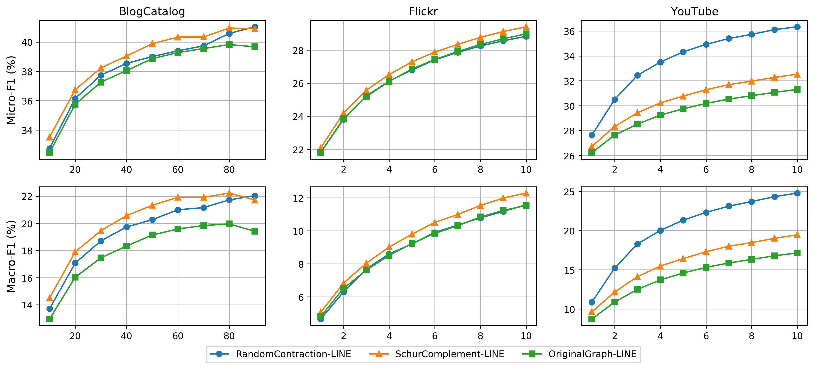
Figure 1: Accuracy of sparsified LINE embeddings. The $x$-axis denotes the training ratio $(\%)$ and the $y$-axis in the top and bottom row denotes the mean Micro-F1 and Macro-F1 scores, respectively.

Results for LINE (NetMF with $W=1$).

We start by evaluating the classification performance of LINE embeddings of the sparsified networks relative to the originals and plot the results across all datasets in Figure 1. Our first observation is that quality of the embedding for classification always improves by running the SchurComplement sparsifier. To explain this phenomenon, we note that LINE computes an embedding using length $W=1$ random walks. This approach, however, is often inferior to methods that use longer random walks such as DeepWalk. When eliminating vertices of a graph using the Schur complement, the resulting graph perfectly preserves random walk transition probabilities through the eliminated vertex set with respect to the original graph. Thus, the LINE embedding of a graph sparsified using SchurComplement implicitly captures longer length random walks through low-degree vertices and hence more structure of the network. For the YouTube experiment, we observe that RandomContraction substantially outperforms SchurComplement and the baseline LINE embedding. We attribute this behavior to the fact that contractions preserve edge sparsity unlike Schur complements. It follows that RandomContraction typically eliminates more nodes than SchurComplement when given a degree threshold. In this instance, the YouTube network sparsified by SchurComplement has 84,371 nodes while RandomContraction produces a network with 53,291 nodes (down from 1,134,890 in the original graph).

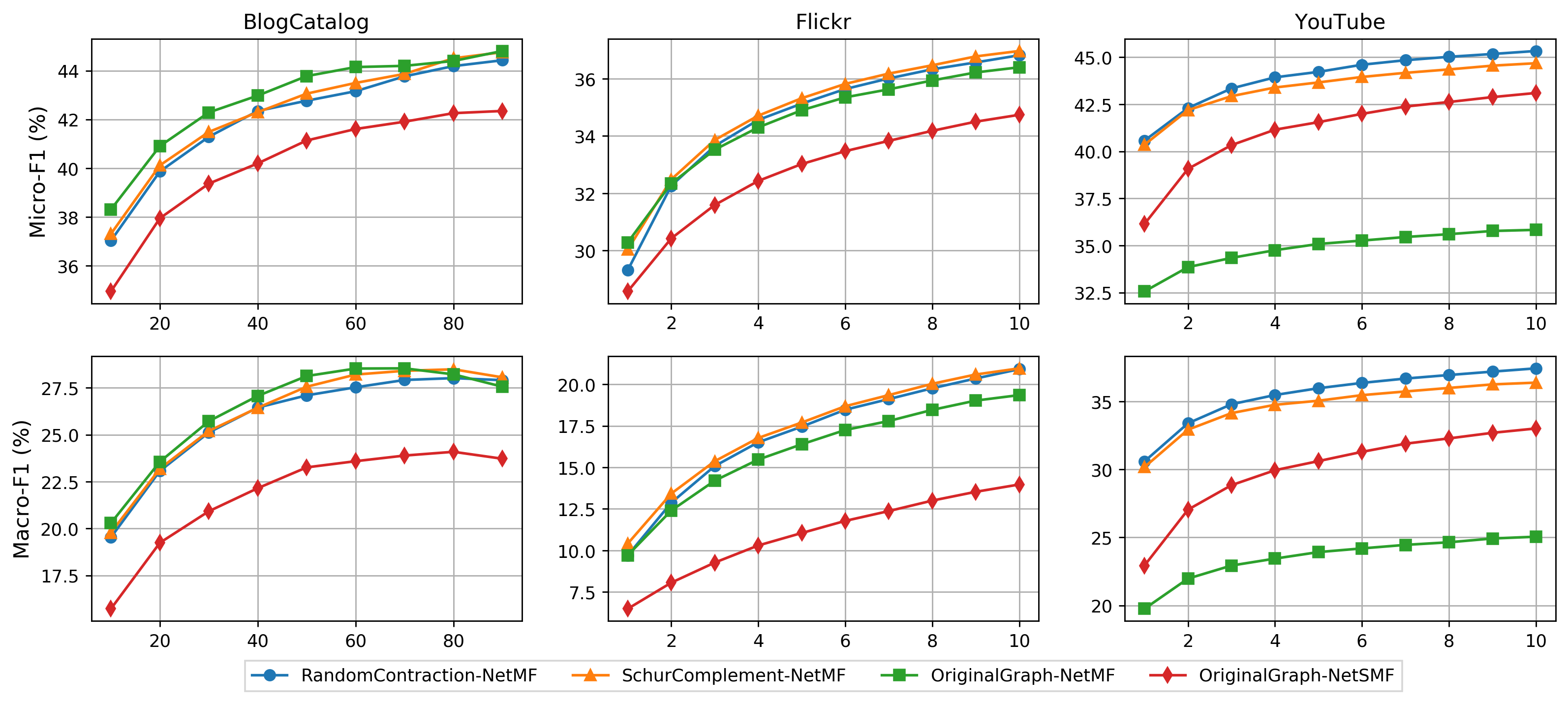
Figure 2: Accuracy of sparsified DeepWalk embeddings. The $x$-axis denotes the training ratio $(\%)$ and the $y$-axis in the top and bottom row denotes the mean Micro-F1 and Macro-F1 scores, respectively.

Results for DeepWalk (NetMF with $W\geq 2$).

Now we consider the same classification experiments using DeepWalk and NetSMF embeddings. We plot the prediction performance for various training ratios across all datasets in Figure 2. Again, we observe that the vertex-sparsified embeddings perform at least as well as the embedding of the original graph for this multi-label classification task, which we attribute to the implicit use of longer random walks. In the YouTube experiment we observe a dramatic improvement over the baseline, but this is because of an entirely different reason than before. A core subroutine of NetMF with $W\geq 2$ is computing the truncated SVD of a dense random walk matrix graph, so the benefits of vertex sparsification surface in two ways. First, the bottleneck in the runtime of the classification pipeline is the truncated SVD. By preprocessing the graph to reduce its vertex set we noticeably speed up this SVD call (e.g., see YouTube and NetMF in Table 2). Second, the convergence rate of the approximate SVD depends on the dimension of the underlying matrix, so the sparsified graphs lead to more accurate eigendecompositions and hence higher quality embeddings. We reiterate that for the YouTube experiment, we set $W=2$ to meet a 432GB memory constraint whereas in the DeepWalk experiments in Perozzi et al., (2014) the authors set $W=10$. We also run NetSMF with $W=10$ on the original graphs as another benchmark, but in some instances we need to use fewer samples to satisfy our memory limit, hence the lower accuracies than in Qiu et al., (2019). When trained on $10\%$ of the label set, SchurComplement achieves 24.45% and 44.67% relative gains over DeepWalk in terms of Micro-F1 and Macro-F1 scores. Furthermore, since RandomContraction yields a coarser graph on fewer nodes, it gives 26.43% and 48.94% improvements relative to DeepWalk.

Table 2: Running times of the coarsening and graph embedding stages in the vertex classification experiment (seconds).

Network	Sparsify	LINE	NetMF	NetSMF
BlogCatalog	–	3.72	20.80	45.56
BlogCatalog SC	1.53	3.88	15.66	–
BlogCatalog RC	2.47	3.83	15.61	–
Flickr	–	51.62	1,007.17	950.60
Flickr SC	19.43	56.62	571.70	–
Flickr RC	59.43	43.41	597.08	–
YouTube	–	147.55	4,714.88	3,458.75
YouTube SC	22.91	44.84	2,053.59	–
YouTube RC	44.13	16.55	909.16	–

5.2 Link Prediction

Datasets.

We build on the experimental framework in node2vec (Grover and Leskovec,, 2016) and evaluate our vertex sparsification algorithms on the following datasets: Facebook (Leskovec and Krevl,, 2014), arXiv ASTRO-PH (Leskovec and Krevl,, 2014), and Protein-Protein Interaction (PPI) (Stark et al.,, 2006). We present the statistics of these networks in Table 3. Facebook is a social network where nodes represent users and edges represent a friendship between two users. The arXiv graph is a collaboration network generated from papers submitted to arXiv. Nodes represent scientists and an edge is present between two scientists if they have coauthored a paper. In the PPI network for Homo Sapiens, nodes represent proteins and edges indicate a biological interaction between a pair of proteins. We consider the largest connected component of the arXiv and PPI graphs.

Table 3: Statistics of the networks in our link prediction experiments.

Dataset	Nodes	Edges
Facebook	4,039	88,234
arXiv ASTRO-PH	17,903	196,972
Protein-Protein Interaction (PPI)	21,521	338,625

Evaluation Methods.

In the terminal link prediction task, we are given a graph and a set of terminal nodes. A subset of the terminal-to-terminal edges are removed, and the goal is to accurately predict edges and non-edges between terminal pairs in the original graph. We generate the labeled dataset of edges as follows: first, randomly select a subset of terminal nodes; to obtain positive examples, remove 50% of the edges chosen uniformly at random between terminal nodes while ensuring that the network is still connected; to obtain negative examples, randomly choose an equal number of terminal pairs that are not adjacent in the original graph. We select 500 (12.4%) nodes as terminals in the Facebook network, 2000 (9.3%) in PPI, and 4000 (22.3%) in arXiv.

For each network and terminal set, we use RandomContraction and SchurComplement to coarsen the graph. Then we compute node embeddings using LINE and NetMF. We calculate an embedding for each edge $(u,v)$ by taking the Hadamard or weighted L2 product of the node embeddings for $u$ and $v$ (Grover and Leskovec,, 2016). Finally, we train a logistic regression model using the edge embeddings as features, and report the area under the receiver operating characteristic curve (AUC) from the prediction scores.

Table 4: Area under the curve (AUC) scores for different operators, coarsening, and embedding algorithms for the link prediction task.

Operator	Algorithm	Facebook	arXiv	PPI
	LINE	0.9891	0.9656	0.9406
	RC + LINE	0.9937	0.9778	0.9431
Hadamard	SC  + LINE	0.9950	0.9854	0.9418
	NetMF	0.9722	0.9508	0.8558
	RC + NetMF	0.9745	0.9752	0.9072
	SC  + NetMF	0.9647	0.9811	0.9018
	LINE	0.9245	0.6129	0.7928
	RC + LINE	0.9263	0.6217	0.7983
Weighted L2	SC  + LINE	0.9523	0.6824	0.7835
	NetMF	0.9865	0.9574	0.8646
	RC + NetMF	0.9852	0.9800	0.9207
	SC  + NetMF	0.9865	0.9849	0.9120

Results.

We summarize our results in Table 4. For all of the datasets, using RandomContraction or SchurComplement for coarsening and LINE with Hadamard products for edge embeddings gives the best results. Moreover, coarsening consistently outperforms the baseline (i.e., the same network and terminals without any sparsification). We attribute the success of LINE-based embeddings in this experiment to the fact that our coarsening algorithms preserve random walks through the eliminated nodes; hence, running LINE on a coarsened graph implicitly uses longer-length random walks to compute embeddings. We see the same behavior with coarsening and NetMF, but the resulting AUC scores are marginally lower. Lastly, our experiments also highlight the importance of choosing the right binary operator for a given node embedding algorithm.

6 Conclusion

We introduce two vertex sparsification algorithms based on Schur complements to be used as a preprocessing routine when computing graph embeddings of large-scale networks. Both of these algorithms repeatedly choose a vertex to remove and add new edges between its neighbors. In Section 4 we demonstrate that these algorithms exhibit provable trade-offs between their running time and approximation quality. The RandomContraction algorithm is faster because it contracts the eliminated vertex with one of its neighbors and reweights all of the edges in its neighborhood, while the SchurComplement algorithm adds a weighted clique between all pairs of neighbors of the eliminated vertex via Gaussian elimination. We prove that the random contraction based-scheme produces a graph that is the same in expectation as the one given by Gaussian elimination, which in turn yields the matrix factorization that random walk-based graph embeddings such as DeepWalk, NetMF and NetSMF aim to approximate.

The main motivation for our techniques is that Schur complements preserve random walk transition probabilities through eliminated vertices, which we can then exploit by factorizing smaller matrices on the terminal set of vertices. We demonstrate on commonly-used benchmarks for graph embedding-based multi-label vertex classification tasks that both of these algorithms empirically improve the prediction accuracy compared to using graph embeddings of the original and unsparsified networks, while running in less time and using substantially less memory.

Appendix A Closure of SDDM Matrices Under the Schur Complement

Lemma A.1.

If $\mathbf{M}$ is an SDDM matrix and $T=V\setminus\{x\}$ is a subset of its columns, then $\mathbf{S}:=\mathbf{SC}(\mathbf{M},T)$ is also an SDDM matrix.

Proof.

Recall that

$$\mathbf{SC}(\mathbf{M},T)=\mathbf{M}_{T,T}-\frac{\mathbf{M}_{T,x}\mathbf{M}^{\top}_{T,x}}{\mathbf{D}^{\prime}_{x,x}},$$

and observe that $\mathbf{D}^{\prime}_{x,x}=\mathbf{M}_{x,x}$. By definition of SDDM matrices, we need to show that $\mathbf{S}$ is (i) symmetric, (ii) its off-diagonal entries are non-positive, and (iii) for all $i\in[n-1]$ we have $\mathbf{S}_{ii}\geq-\sum_{j\neq i}\mathbf{S}_{ij}$. An easy inspection shows that $\mathbf{S}$ satisfies (i) and (ii). We next show that (iii) holds.

To this end, by definition of $\mathbf{S}$, we have that

$$-\sum_{j\neq i}\mathbf{S}_{ij} =\sum_{j\neq i}\left(-\mathbf{M}_{ij}+\frac{\mathbf{M}_{ix}\mathbf{M}_{xj}}{\mathbf{M}_{xx}}\right)$$

$$=-\sum_{j\neq i}\mathbf{M}_{ij}+\frac{\mathbf{M}_{ix}}{\mathbf{M}_{xx}}\left(\sum_{j\neq i}\mathbf{M}_{xj}\right)$$ (9)

As $\mathbf{M}$ is an SDDM matrix, the following inequality holds for the $x$-th row of $\mathbf{M}$

$$-\sum_{j\neq i}\mathbf{M}_{xj}\leq\mathbf{M}_{ix},$$

or equivalently

$$\mathbf{M}_{ix}\left(\sum_{j\neq i}\mathbf{M}_{xj}\right)\leq-\mathbf{M}^{2}_{ix}.$$ (10)

Plugging Eq. (10) in Eq. (A) and using the fact that $-\sum_{j\neq i}\mathbf{M}_{ij}\leq\mathbf{M}_{ii}$, we get that

$$-\sum_{j\neq i}\mathbf{S}_{ij} \leq\mathbf{M}_{ii}-\frac{\mathbf{M}^{2}_{ix}}{\mathbf{M}_{xx}}=\mathbf{S}_{ii},$$

which completes the proof of the lemma. ∎

References

- Abu-El-Haija et al., (2019) Abu-El-Haija, S., Perozzi, B., Kapoor, A., Alipourfard, N., Lerman, K., Harutyunyan, H., Steeg, G. V., and Galstyan, A. (2019). MixHop: Higher-order graph convolutional architectures via sparsified neighborhood mixing. In Proceedings of the 36th International Conference on Machine Learning, pages 21–29. PMLR.
- Batson et al., (2013) Batson, J., Spielman, D. A., Srivastava, N., and Teng, S.-H. (2013). Spectral sparsification of graphs: Theory and algorithms. Communications of the ACM, 56(8):87–94.
- Benson and Kleinberg, (2019) Benson, A. and Kleinberg, J. (2019). Link prediction in networks with core-fringe data. In Proceedings of the 28th International Conference on World Wide Web, pages 94–104. ACM.
- Borgatti and Everett, (2000) Borgatti, S. P. and Everett, M. G. (2000). Models of core/periphery structures. Social networks, 21(4):375–395.
- Briggs et al., (2000) Briggs, W. L., Henson, V. E., and McCormick, S. F. (2000). A Multigrid Tutorial. SIAM.
- Bringmann and Panagiotou, (2017) Bringmann, K. and Panagiotou, K. (2017). Efficient sampling methods for discrete distributions. Algorithmica, 79(2):484–508.
- Bruna et al., (2014) Bruna, J., Zaremba, W., Szlam, A., and LeCun, Y. (2014). Spectral networks and locally connected networks on graphs. In Proceedings of the 2nd International Conference on Learning Representations.
- Cao et al., (2015) Cao, S., Lu, W., and Xu, Q. (2015). GraRep: Learning graph representations with global structural information. In Proceedings of the 24th ACM International Conference on Information and Knowledge Management, pages 891–900.
- Chen et al., (2018) Chen, H., Perozzi, B., Hu, Y., and Skiena, S. (2018). HARP: Hierarchical representation learning for networks. In Proceedings of the Thirty-Second AAAI Conference on Artificial Intelligence, pages 2127–2134.
- Cheng et al., (2015) Cheng, D., Cheng, Y., Liu, Y., Peng, R., and Teng, S.-H. (2015). Efficient sampling for Gaussian graphical models via spectral sparsification. In Proceedings of The 28th Conference on Learning Theory (COLT), pages 364–390. PMLR.
- Chevalier and Safro, (2009) Chevalier, C. and Safro, I. (2009). Comparison of coarsening schemes for multilevel graph partitioning. In International Conference on Learning and Intelligent Optimization, pages 191–205. Springer.
- Cummings et al., (2019) Cummings, R., Fahrbach, M., and Fatehpuria, A. (2019). A fast minimum degree algorithm and matching lower bound. arXiv preprint arXiv:1907.12119.
- Englert et al., (2014) Englert, M., Gupta, A., Krauthgamer, R., Räcke, H., Talgam-Cohen, I., and Talwar, K. (2014). Vertex sparsifiers: New results from old techniques. SIAM J. Comput., 43(4):1239–1262.
- Fahrbach et al., (2018) Fahrbach, M., Miller, G. L., Peng, R., Sawlani, S., Wang, J., and Xu, S. C. (2018). Graph sketching against adaptive adversaries applied to the minimum degree algorithm. In 2018 IEEE 59th Annual Symposium on Foundations of Computer Science (FOCS), pages 101–112. IEEE.
- George and Liu, (1989) George, A. and Liu, J. W. H. (1989). The evolution of the minimum degree ordering algorithm. SIAM Review, 31(1):1–19.
- Grover and Leskovec, (2016) Grover, A. and Leskovec, J. (2016). Node2vec: Scalable feature learning for networks. In Proceedings of the 22nd ACM SIGKDD International Conference on Knowledge Discovery and Data Mining, page 855–864.
- Hamilton et al., (2017) Hamilton, W. L., Ying, Z., and Leskovec, J. (2017). Inductive representation learning on large graphs. In Advances in Neural Information Processing Systems, pages 1024–1034.
- Jia and Benson, (2019) Jia, J. and Benson, A. R. (2019). Random spatial network models for core-periphery structure. In Proceedings of the Twelfth ACM International Conference on Web Search and Data Mining, pages 366–374. ACM.
- Karypis and Kumar, (1998) Karypis, G. and Kumar, V. (1998). A software package for partitioning unstructured graphs, partitioning meshes, and computing fill-reducing orderings of sparse matrices.
- Kipf and Welling, (2017) Kipf, T. N. and Welling, M. (2017). Semi-supervised classification with graph convolutional networks. In Proceedings of the 5th International Conference on Learning Representations.
- Kyng et al., (2016) Kyng, R., Lee, Y. T., Peng, R., Sachdeva, S., and Spielman, D. A. (2016). Sparsified cholesky and multigrid solvers for connection laplacians. In Proceedings of the 48th Annual ACM SIGACT Symposium on Theory of Computing (STOC), pages 842–850.
- Kyng and Sachdeva, (2016) Kyng, R. and Sachdeva, S. (2016). Approximate gaussian elimination for laplacians - fast, sparse, and simple. In 2016 IEEE 57th Annual Symposium on Foundations of Computer Science (FOCS), pages 573–582.
- Leskovec and Krevl, (2014) Leskovec, J. and Krevl, A. (2014). SNAP Datasets: Stanford large network dataset collection. http://snap.stanford.edu/data.
- Liang et al., (2018) Liang, J., Gurukar, S., and Parthasarathy, S. (2018). MILE: A multi-level framework for scalable graph embedding. arXiv preprint arXiv:1802.09612.
- Lipton et al., (1979) Lipton, R. J., Rose, D. J., and Tarjan, R. E. (1979). Generalized nested dissection. SIAM Journal on Numerical Analysis, 16(2):346–358.
- Liu et al., (2016) Liu, Y., Dighe, A., Safavi, T., and Koutra, D. (2016). A graph summarization: A survey. CoRR, abs/1612.04883.
- Loukas and Vandergheynst, (2018) Loukas, A. and Vandergheynst, P. (2018). Spectrally approximating large graphs with smaller graphs. In Proceedings of the 35th International Conference on Machine Learning, pages 3237–3246. PMLR.
- Moitra, (2009) Moitra, A. (2009). Approximation algorithms for multicommodity-type problems with guarantees independent of the graph size. In 50th Annual IEEE Symposium on Foundations of Computer Science (FOCS), pages 3–12.
- Pedregosa et al., (2011) Pedregosa, F., Varoquaux, G., Gramfort, A., Michel, V., Thirion, B., Grisel, O., Blondel, M., Prettenhofer, P., Weiss, R., Dubourg, V., et al. (2011). Scikit-learn: Machine learning in Python. Journal of Machine Learning Research, 12:2825–2830.
- Perozzi et al., (2014) Perozzi, B., Al-Rfou, R., and Skiena, S. (2014). Deepwalk: Online learning of social representations. In Proceedings of the 20th ACM SIGKDD International Conference on Knowledge Discovery and Data Mining, pages 701–710. ACM.
- Qiu et al., (2019) Qiu, J., Dong, Y., Ma, H., Li, J., Wang, C., Wang, K., and Tang, J. (2019). NetSMF: Large-scale network embedding as sparse matrix factorization. In Proceedings of the 28th International Conference on World Wide Web, pages 1509–1520. ACM.
- Qiu et al., (2018) Qiu, J., Dong, Y., Ma, H., Li, J., Wang, K., and Tang, J. (2018). Network embedding as matrix factorization: Unifying deepwalk, line, pte, and node2vec. In Proceedings of the Eleventh ACM International Conference on Web Search and Data Mining, pages 459–467.
- Stark et al., (2006) Stark, C., Breitkreutz, B.-J., Reguly, T., Boucher, L., Breitkreutz, A., and Tyers, M. (2006). BioGRID: A general repository for interaction datasets. Nucleic Acids Research, 34:D535–D539.
- Tang et al., (2015) Tang, J., Qu, M., Wang, M., Zhang, M., Yan, J., and Mei, Q. (2015). LINE: Large-scale information network embedding. In Proceedings of the 24th International Conference on World Wide Web, pages 1067–1077.
- Tang and Liu, (2009) Tang, L. and Liu, H. (2009). Relational learning via latent social dimensions. In Proceedings of the 15th ACM SIGKDD International Conference on Knowledge Discovery and Data Mining, pages 817–826. ACM.
- Tang and Liu, (2011) Tang, L. and Liu, H. (2011). Leveraging social media networks for classification. Data Mining and Knowledge Discovery, 23(3):447–478.
- Thorup and Zwick, (2005) Thorup, M. and Zwick, U. (2005). Approximate distance oracles. J. ACM, 52(1):1–24.
- Vattani et al., (2011) Vattani, A., Chakrabarti, D., and Gurevich, M. (2011). Preserving personalized pagerank in subgraphs. In Proceedings of the 28th International Conference on Machine Learning, page 793–800.
- Veličković et al., (2018) Veličković, P., Cucurull, G., Casanova, A., Romero, A., Lio, P., and Bengio, Y. (2018). Graph attention networks. In Proceedings of the 6th International Conference on Learning Representations.
- Viswanathan et al., (2019) Viswanathan, K., Sachdeva, S., Tomkins, A., and Ravi, S. (2019). Improved semi-supervised learning with multiple graphs. In The 22nd International Conference on Artificial Intelligence and Statistics, pages 3032–3041.
- Wagner et al., (2018) Wagner, T., Guha, S., Kasiviswanathan, S., and Mishra, N. (2018). Semi-supervised learning on data streams via temporal label propagation. In Proceedings of the 35th International Conference on Machine Learning, pages 5095–5104.
- Yang and Leskovec, (2015) Yang, J. and Leskovec, J. (2015). Defining and evaluating network communities based on ground-truth. Knowledge and Information Systems, 42(1):181–213.
- Yang et al., (2016) Yang, Z., W. Cohen, W., and Salakhutdinov, R. (2016). Revisiting semi-supervised learning with graph embeddings. In Proceedings of the 33rd International Conference on Machine Learning, pages 40–48.