Signatures of Long-Range Spin-Triplet Component in Andreev Interferometer

Abstract

We analyze the Josephson,$I_{J}$, and dissipative,$I_{V}$, currents in a magnetic Andreev interferometer in the presence of the long-range spin triplet component (LRSTC). Andreev interferometer has a cross-like geometry and consists of a SF_l - F - F_rS circuit and perpendicular to it a N - F - N circuit, where S, F_l,r are superconductors and weak ferromagnets with non-collinear magnetisations $\mathbf{M}_{l,r}$, F is a strong ferromagnet. The ferromagnetic wire F can be replaced with a non-magnetic wire n. In the limit of a weak proximity effect (PE), we obtain simple analytical expressions for the currents $I_{J}$ and $I_{V}$. In particular, the critical Josephson current in a long Josephson junction (JJ) is $I_{c}(\alpha,\beta)=I_{0c}\chi(\alpha,\beta)$, where the function $\chi(\alpha,\beta)$ is a function of angles $(\alpha,\beta)_{l,r}$ that characterize the orientations of $\mathbf{M}_{l,r}$. The oscillating part of the dissipative current $I_{osc}(V)=\chi(\alpha,\beta)\cos\varphi I_{0}(V)$ in the N - F(n)- N circuit depends on the angles $(\alpha,\beta)_{l,r}$ in the same way as the critical Josephson current $I_{c}(\alpha,\beta)$, but can be much greater than the $I_{c}(\alpha,\beta)$. At some angles the current $I_{c}(\alpha,\beta)$ changes sign. We briefly discuss a relation between the negative current $I_{c}$ and paramagnetic response. We argue that the measurements of the conductance in N - F(n) - N circuit can be used as another complementary method to identify the LRSTC in S/F heterostructures.

I Introduction

The phenomenon of phase coherence in superconducting systems is especially well studied in Josephson junctions (JJs). In particular, if the magnetic flux $\Phi$ of an external magnetic field $H_{ex}$ in a JJ with planar geometry is equal to an integer number of the flux quanta $\Phi_{0}=hc/2e$ ($\Phi=n\Phi_{0}$), the Josephson current $I_{J}$ turns periodically to zero KulikBook70 ; LikharevRMP79 ; BaroneBook82 . Another example of phase coherence are the so-called Shapiro steps that arise on the $I-V$ characteristics in a JJ irradiated by an $ac$ electromagnetic field with a frequency $\omega$. The positions of the steps $V_{n}$ is defined by the condition $V_{n}=n\hbar\omega/2e$. Since the discovery of Josephson effect Josephson62 , various aspects of this effect have been intensively studied on JJs of different types such as SIS, SNS, ScS junctions, where S, N, c stand for a superconductor, normal metal and constriction, respectivelyKulikBook70 ; LikharevRMP79 ; BaroneBook82 .

In the last few decades a great attention was paid to the study of magnetic JJs, i.e. SFS junctions, where the Josephson coupling is realized via a ferromagnetic layer(s) F. A number of interesting phenomena have been predicted and observed in such JJs. One of them is the sign-reversal of the Josephson critical current with changing temperature or thickness of the F layer GolubovRMP04 ; BuzdinRev05 ; BVErev05 ; EschrigRev11 ; LinderRev15 . This effect was originally predicted back in the 80s of the 20th century Bulaev77 ; Bulaev82 ; BuzdinKup90 ; BuzdinKup91 , but was observed experimentally only much later RyazanovPRL01 ; RyazanovPRL06 ; ApriliPRL02 ; SellierPRB03 ; Weides06 .

Another interesting feature of magnetic JJs is the appearance of the so-called long-range spin triplet component (LRSTC) of the condensate BuzdinRev05 ; BVErev05 ; EschrigRev11 ; LinderRev15 ; LinderBalRMP17 . The triplet component is induced by proximity effect in the F layer in any magnetic JJs due to Zeeman interaction of quasiparticles, which build Cooper pairs, with an exchange field of a ferromagnet. However, a uniform exchange field produces only a short-ranged component, which quickly decays inside the F layer. The wave function of this component, $f$, is given by $f(t,t^{\prime})$ $\sim\langle\psi_{\uparrow}(t)\psi_{\downarrow}(t^{\prime})+\psi_{\downarrow}(t^{\prime})\psi_{\uparrow}(t)\rangle$ and its spin is perpendicular to the magnetization vector $\mathbf{M}$ in F. Such pairs penetrate ferromagnet on a short distance of the order $\xi_{F}\cong\sqrt{D_{F}/E_{F}}$, where $D_{F}$ is the diffusion coefficient in F and $E_{F}$ is the exchange energy. In addition, this penetration is accompanied by oscillations of $f(x)$ in space. At the same time, the actual LRSTC described by the wave functions $f\sim\langle\psi_{\uparrow}(t)\psi_{\uparrow}(t^{\prime})\rangle$ or $f\sim\langle\psi_{\downarrow}(t)\psi_{\downarrow}(t^{\prime})\rangle$ occurs in magnetic JJs with a non-uniform magnetization $\mathbf{M}(\mathbf{r})$ in the F film BVEprl01 ; Footnote ; BuzdinRev05 ; BVErev05 ; EschrigRev11 ; LinderRev15 ; LinderBalRMP17 . The penetration depth of the LRSTC into a ferromagnet is much longer than $\xi_{F}$ and may be of the order of the Cooper pair penetration length into a normal metal, $\xi_{T}=\sqrt{D_{F}/2\pi T}$. The prediction of a long-range penetration of the triplet Cooper pairs into a ferromagnet was observed in multiple experiments KlapwijkNature06 ; SosninVolkovPRL06 ; BirgePRL10 ; BlamireScience10 ; ZabelPRB10 ; AartsPRB10 ; BlamirePRL10 ; PetrashovZaikinPRL11 ; BirgePRL16 ; BirgePRB18 ; BlamirePRB18 . Observe that both components, long- and short-range, can be described by the Fourier transform, $f_{\omega}$, of the function $f(t,t^{\prime})$ which should be an odd function of $\omega$ to satisfy the Pauli principle, i.e. $f(t,t)=0$ BuzdinRev05 ; BVErev05 ; EschrigRev11 ; LinderRev15 . The sign reversal of the critical Josephson current $I_{c}$ may be then related both to the short-range (see reviews GolubovRMP04 ; BuzdinRev05 ; LinderRev15 ) and long-range triplet components BVEprl03 ; AnischPRB06 ; EschrigPRB07 ; EschrigPRL08 ; Kawabata10 ; GolubovPRL10 ; HaltermanPRB14 ; HaltermanPRB15 ; BlamirePRL19 . The interest in the study of magnetic JJs is caused not only by new physical effects, but also by possible applications of these junctions in spintronics (see review LinderRev15 as well as recent papers Birge20 ; Blamire20 ; BlamireBuzdin20 and references therein) or in Josephson magnetic random access memory Birge19 .

Although it is less known outside of the community, the phase coherence takes place not only in JJs, but also in multi-terminal superconducting structures like the so-called Andreev interferometers (see Fig.1), which for a number of applications may have several important advantages over some devices based on JJs Petrashov94 ; KlapwijkPRL96 ; TakayanVolkovPRL96 ; PannetierPRL96 ; PannVolkovPRL96 ; PetrashovPRL99 ; PetrashovPRB00 ; PetrashovPRL05 ; ErvandPRB10 ; ZaikinPRB12 ; GiazottoPRB17 ; ZaikinPRB19 . It has been found that the conductance between the N-reservoirs oscillates with variation of the phase difference $\varphi$ between the superconducting reservoirs S. The phase variation is provided either by passing a $dc$ current between S reservoirs or by an external magnetic field $H_{ext}$ applied in a superconducting loop connecting the S reservoirs. Beside the conductance oscillations other interesting phenomena may arise in Andreev interferometers TakayanVolkovPRL96 ; KlapwijkPRL96 ; PetrashovPRB00 ; PetrashovPRL05 ; ZaikinPRB12 ; GiazottoPRB17 ; ZaikinPRB19 like the change of sign of the Josephson critical current $I_{c}$ in multiterminal S-n-N structures. In contrast to the change of sign discussed above for the magnetic JJs, here it is related to an imbalance between the condensate and the quasiparticles in the S-n-S circuit out-of-equilibrium. The effect of sign inversion in S-n-S JJs has been considered in Refs. BagwellPRB97 in ballistic JJs (see also references in ShumeikoPRB03 ). In the more practical case of diffusive JJs the sign change effect has been predicted in VolkovPRL95 (for further development of this idea, see Refs.ZaikinPRL98 ; Yip98 ; Bobkov10 ; Bobkov12 ). The predicted effect has been observed by the Klapwijk group vanWees02 ; KlapwijkNat06 . The voltage $V$ applied between N and S reservoirs leads to a non-equilibrium distribution function $n(V)$ which affects strongly the current $I_{c}$ if $V\approx\Delta/e$.

Despite of numerous studies of various phenomena in magnetic superconducting heterostructures, the LRSTC in Andreev interferometer remains largely unexplored except for the conductance analysis in an interferometer-like (three-terminal) superconducting system with a topological insulator and in presence of a spin-orbit and Zeeman interactions Mal'shukovPRB18 . In this manuscript we study the propagation of the LRSTC in an Andreev interferometer and its influence on the conductance $G_{NN}$ of the N - F(n) - N circuit as well as on the Josephson current $I_{J}$. As we are mostly interested in propagation of the LRSTC, our results are equally applied for the normal (n) or ferromagnetic (F) wire between the reservoirs S or N. It is only assumed that its length, $L_{x}$, is larger than $\xi_{F}$ such that only the LRSTC penetrates the F wire. Note also, that in the case of SF_l - n - F_rS junction (horizontal line), not only the LRSTC penetrates in the n-wire but also a spin singlet component.

The calculations are carried out in the approximation of a weak PE. We show that the conductance $G_{NN}$ contains a part $G_{osc}$ which oscillates with the increase of the phase difference $\varphi$: $G_{osc}=G_{0}\chi(\alpha,\beta)\cos\varphi$, where $\chi(\alpha,\beta)$ is a function of the angles $(\alpha,\beta)$ which characterize the magnetization vectors in the ferromagnetic layers $F_{l,r}$.(see Eq.(43)). The Josephson current $I_{J}=I_{c}(\alpha,\beta)\sin\varphi$ has the standard phase dependence with the critical current $I_{c}(\alpha,\beta)$ which has the same angle dependence as $G_{osc}(\alpha,\beta)$. In the case of SF_l - F - F_r structure, the critical current turns to zero at $\alpha_{l}=\alpha_{r}\pm\pi/2$ and any $\beta$ or at $\beta_{l,r}=0$ and any $\alpha$. We further discuss the relation between negative $I_{c}$ and a paramagnetic response.

II Basic Equations

We consider the structure shown in Fig.1. It consists of two superconducting S and two normal-metal N reservoirs, respectively. They are connected by ferromagnetic (normal) wires of length, $L$. The superconductors are covered by thin magnetic layers. These layers are made of weak ferromagnets F_l,r whereas the wire between N or S reservoirs consists of a strong ferromagnet F_st or normal (non-magnetic) metal. The magnetization vector $\mathbf{M}_{l,r}=(M\mathbf{n)}_{l,r}$ in the weak ferromagnets are expected to be not collinear with respect to each other and to the magnetization $\mathbf{M}_{st}=M_{st}\mathbf{n}_{z}$ in the magnetic wire so that the LRSTC arises in the structure due to proximity effect (PE) BVEprl01 ; BVErev05 ; EschrigRev11 ; LinderRev15 . The unit vector $\mathbf{n}$ is characterized by the polar ($\beta$) and the azimuthal ($\alpha$) angles in the usual way $\mathbf{n}=(\sin\beta\cos\alpha$, $\sin\beta\sin\alpha$, $\cos\beta)$. In particular, non-collinearity means that $\beta\neq 0$ and $\alpha_{l}\neq\alpha_{r}$. In principle, for LRSTC penetration it should not matter whether the F wire is magnetic or non-magnetic yet in practice possible magnetic inhomogeneities in the F wire may shorten the penetration length of the LRSTC IvanovFominSkvorts09 . In what follows we calculate the conductance between the N reservoirs, $G$, and its deviation due to the PE from that in the normal state (above $T_{c}$) $G_{nor}$. The voltages in the N reservoirs are assumed to be $\pm V$, the electric potential in the S reservoirs is set to zero and their phases are different and equal to $\pm\varphi/2$. In the considered symmetric N - F(n) - N circuit the electric potential $V$ equals zero in the center of the cross, i.e. $V(y)=0$ at $y=0$, such that there is no voltage difference between the S-F(n)-S superconducting circuit and the N - F(n) - N circuit. In this respect, the case considered here differs from that studied in Ref.VolkovPRL95 , where a voltage drop between the center of the $x$-circuit ($V(x)$ at $x=0$) and the S reservoirs was of the order of $\Delta/e$. This means that, unlike the current situation, the quasiparticles in the S-F(n)-S circuit, considered in Ref.VolkovPRL95 were not in equilibrium with condensate.

The calculations are carried out on the basis of equations for generalized quasiclassical Green’s functions $\check{G}$ LOrev ; VZK93 ; ZaitsevVolkov99 ; ZaikinBelzig99 ; KopninBook , which are widely and successfully used in the theory of S/N or S/F structures VZK93 ; Zaitsev94 ; NazarovStoof96 ; Zaikin97 ; ZaitsevVolkov99 . Here, the elements of the matrix $\check{G}$ are the retarded (advanced) Green’s functions $\check{g}^{R(A)}=\check{G}_{11,22}$ as well as the Keldysh function $\check{g}=\check{G}_{12}$, which in turn are also matrices in the Gor’kov-Nambu ($\hat{\tau}$ matrices) and the spin ($\sigma$ matrices) space, respectively. In particular, the Keldysh function $\check{g}$ is written in terms of matrix distribution functions $\check{n}$

$$\check{g}=\check{g}^{R}\cdot\check{n}-\check{n}\cdot\check{g}^{A}$$ (1)

where the matrix $\check{n}$ can be represented as

$$\check{n}=\hat{n}_{od}\cdot\hat{\tau}_{0}+\hat{n}_{ev}\cdot\hat{\tau}_{3}$$ (2)

where $\hat{n}_{od}$ and $\hat{n}_{ev}$ are matrices in the spin space and $\tau_{i}$ are matrices in the Gor’kov-Nambu space. The reservoirs S and N are supposed to be in equilibrium so that the distribution functions $\hat{n}_{od,ev}=\hat{\sigma}n_{odd,ev}$ are equal to

$$n_{od}=\tanh(\epsilon/2T)\text{, }n_{ev}=0;$$ S reservoirs,

$$n_{od,ev}(L_{y})=F_{\pm}(V);$$ N reservoir at the top, (3)

$$\hat{n}_{nod,ev}(-L_{y})=F_{\pm}(-V);$$ N reservoir at the bottom,

where $F_{\pm}(\epsilon,V)=\frac{1}{2}[\tanh((\epsilon+eV)/2T)\pm\tanh((\epsilon-eV)/2T]$. The subscripts $ev,odd$ denote even (odd) functions of the energy $\epsilon$, respectively. $\check{g}$, $\check{g}^{R(A)}$ also obey the normalization condition

$$\check{g}^{R}\cdot\check{g}+\check{g}\cdot\check{g}^{A} = 0,$$ (4)

$$\check{g}^{R(A)}\cdot\check{g}^{R(A)} = \check{1}$$ (5)

In the F wire the matrices $\check{g}$ and $\check{g}^{R(A)}$ satisfy the generalized Usadel equation LOrev ; VZK93 ; ZaikinBelzig99 ; KopninBook

$$D_{v}\nabla(\check{g}^{R}\cdot\nabla\check{g}+\check{g}\cdot\nabla\check{g}^{A})+i\epsilon[\hat{\tau}_{3}\cdot\hat{\sigma}_{0},\check{g}]+i\kappa_{F}[\hat{\tau}_{3}\cdot\hat{\sigma}_{3},\check{g}] = 0\text{,}$$ (6)

$$D_{v}\nabla(\check{g}\cdot\nabla\check{g})^{R(A)}+i\epsilon[\hat{\tau}_{3}\cdot\hat{\sigma}_{0},\check{g}^{R(A)}]+i\kappa_{F}[\hat{\tau}_{3}\cdot\hat{\sigma}_{3},\check{g}^{R(A)}] = 0\text{ }$$ (7)

where $\kappa_{F}=\sqrt{E_{F}sign(\omega)/D_{F}}$ is a parameter which characterizes a decay of the short-range component in the F film. In the case

Observe that if the wires connecting S and N reservoirs are non-magnetic (n metals), the last terms vanishes. The charge current density $I$ in a wire with conductivity $\sigma$ is expressed conventionally in terms of matrices $\check{G}$ and is a sum of the condensate current $I_{S}$ and the quasiparticle current $I_{qp}$, $I=I_{S}+I_{qp}$, as follows

$$I=\frac{\sigma}{4e}\int d\epsilon\{\check{g}^{R}\cdot\partial_{x}\check{g}+\check{g}\cdot\partial_{x}\check{g}^{A}\}_{3,0}$$ (8)

where $\{(..)\}_{3,0}\equiv$ Tr$\{(\hat{\sigma}_{0}\cdot\hat{\tau}_{3})\cdot(..)\}/4$. In the symmetric case, considered here, only $I_{S}$ differs from zero in the $x$-wire. It is proportional to $\hat{n}_{eq}=\hat{\sigma}_{0}\tanh(\epsilon/2T)$ and, as follows from Eq.(8), is expressed in terms of the condensate functions $\check{f}_{\omega}$

$$I_{S} = \frac{\sigma_{x}}{4e}\int d\epsilon\{(\check{g}^{R}\cdot\partial_{x}\check{g}^{R}-\check{g}^{A}\cdot\partial_{x}\check{g}^{A})\hat{n}_{eq}\}_{3,0}=$$ (9)

$$= i\pi\sigma_{x}\frac{T}{e}\sum_{\omega\geqslant 0}\{\check{f}_{\omega}\cdot\partial_{x}\check{f}_{\omega}\}_{3,0}\text{.}$$ (10)

where $\sigma_{x,y}$ are conductivities in the $x$- and $y$- wires, the condensate Green’s function $\check{f}^{R(A)}$ are defined below (see Eq.(11)); they anticommutes with the matrix $\hat{\tau}_{3}\cdot\hat{\sigma}_{0}$. Eq.(10) is identical to Eq.(9) in the Matsubara representation with $\omega=\pi T(2n+1)$. Here we represent $\check{g}^{R(A)}$ functions as follows

$$\check{g}^{R(A)}=\hat{g}^{R(A)}\hat{\tau}_{3}+\check{f}^{R(A)}$$ (11)

The condensate matrix Green’s functions $\check{f}^{R(A)}$ have the form $\check{f}^{R(A)}=\hat{\tau}_{\perp}\hat{f}^{R(A}$ with $\hat{\tau}_{\perp}\sim\hat{\tau}_{1,2}$ (see next section). In the vertical wire there is no supercurrent and the current $I_{y}$ is carried by quasiparticles. Eq. (8) can be written as

$$I_{y}=\frac{\sigma_{y}}{4e}\int d\epsilon\partial_{y}\{\hat{n}_{ev}\}_{0}[1-\{\check{g}^{R}\cdot\hat{\tau}_{3}\cdot\check{g}^{A}\}_{3,0}]=\frac{\sigma_{y}T}{eL_{y}}\int d\zeta\tilde{J}(\zeta)\text{ }$$ (12)

where $\{\hat{n}_{ev}\}_{0}\equiv(1/2)$Tr$(\hat{\sigma}_{0}\hat{n}_{ev})$ and $\zeta=\epsilon/(2T)$. Using Eq.(11), we can represent the partial current $J(\epsilon)$ in the following form

$$\tilde{J}(\zeta,y)\text{ }=\frac{L_{y}}{2}(\partial_{y}n_{0})(1-m(\zeta,y))$$ (13)

where $n_{0}=\{\hat{n}_{ev}\}_{0}$ and

$$m(\zeta,y)=\frac{1}{4}\{[\check{f}^{R}(\zeta,y)-\check{f}^{A}(\zeta,y)]^{2}\}_{0,0}$$ (14)

Here, we use the approximation $\check{g}^{R(A)}\approx\pm(1+(1/2)(\check{f}^{R(A)})^{2})$, which follows from Eq.(5) in the case of a weak PE, i. e., $|\check{f}^{R(A)}(y)|\ll 1$. Thus, the product $(\hat{g}^{R}\cdot\hat{g}^{A})_{0}$ is equal to

$$-(\hat{g}^{R}(\zeta,y)\cdot\hat{g}^{A}(\zeta,y))_{0}\cong 1+\{\frac{1}{2}(\hat{f}^{R}(\zeta,y)+\hat{f}^{A}(\zeta,y))^{2}\}_{0}\text{,}$$ (15)

Thus, the currents $I_{x,y}$ are given by Eq.(10) and Eqs.(11-14), respectively. In order to evaluate further these currents, we need to determine the condensate Green’s functions $\check{f}^{R(A)}$ in the $x$- and $y$-wires. This we do in the next section.

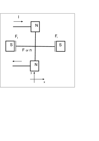
Figure 1: (Color online.) Schematic structure of the system under consideration. The current $I$ is the dissipative current in the vertical circuit.

III Condensate Green’s Functions

III.1 Condensate Functions in the x-Wire

In order to simplify the calculation, we assume that the interface resistance of the cross is larger than the resistance of the F_x,y or n_x,y wires, i. e.

$$R_{B}/w_{x,y}\gg L_{x,y}/\sigma_{x,y}\text{,}$$ (16)

where $R_{B}$ is the resistance of the interface between $x$ - and $y$-wires per unit area, $w_{x,y}$ is the width of these wires. This assumption means that when determining the condensate function in the $x$-wire, we can neglect the leakage of Cooper pairs from the $x$-wire into the $y$-wire. On the other hand, the condensate into the $y$-wire is determined by a small leakage from the $x$ wire. The generalization for the case of arbitrary $R_{B}$ is straightforward and does not change the results qualitatively.

In what follows we evaluate the condensate function $\check{f}_{\omega}(x,y)$ in the $x$- and $y$-wires. In the SF_l - n(F) - F_rS wire, the condensate functions in the Matsubara representation $\check{f}_{\omega}(x,0)$ obey the linearized Usadel equation, Eq.(7)

$$-\partial_{xx}^{2}\check{f}_{\omega}+\kappa_{\omega}^{2}\check{f}_{\omega}+i(\kappa_{F}^{2}/2)[\hat{\sigma}_{3},\check{f}_{\omega}]_{+}+i(\kappa_{l}/2)\delta(x+L_{x})[\hat{\sigma}_{1},\check{f}_{\omega}]_{+}+i(\kappa_{r}/2)\delta(x-L_{x})[\hat{\sigma}_{r},\check{f}_{\omega}]_{+}=0\text{,}$$ (17)

where $\kappa_{\omega}^{2}=2|\omega|/D_{F}$, $\kappa_{F}^{2}=E_{F}$sign $(\omega)/D_{F}$, $\kappa_{l,r}=(wE)_{l,r}\mbox{sign}(\omega)/D_{F}$. Here, $E_{H}$ and $E_{l,r}$ are the exchange energy in the strong or left (right) ferromagnetic films, respectively, $w$ is the thickness of the F_l,r films. The matrices $\hat{\sigma}_{l,r}\equiv(\mathbf{\hat{\sigma}n})_{l,r}$are defined in the following way

$$\hat{\sigma}_{l,r}=\{(\hat{\sigma}_{1}\cos\alpha+\hat{\sigma}_{2}\sin\alpha)\sin\beta+\hat{\sigma}_{3}\cos\beta\}_{l,r}.$$ (18)

The unit vector $\mathbf{n}$ has the components $\mathbf{n}_{l,r}=(\cos\alpha\sin\beta$,$\sin\alpha\sin\beta$,$\cos\beta)_{l,r}$. It is important to note that the spin and the orbital degree of freedom are decoupled in our model as no spin-orbit interaction is included. Therefore, the components of the vectors $\mathbf{n}_{l,r}=(n_{x},n_{y}$,$n_{z})$ are arbitrarily oriented independent of the coordinate system shown in Fig.1. In particular, we would like to stress that the magnetisation vector $\mathbf{M}=M_{0}\mathbf{n}$ is not necessarily oriented along the $x$-axis shown in Fig.1 if $\alpha=0$ and $\beta=\pi/2$. The $\delta$-functions in Eq.(17) refer to the thickness of the F_l,r layers, $w_{l,r}$, which is assumed to be is thinner than $\kappa_{l,r}^{-1}$. In addition, Eq.(17) is supplemented by boundary conditions ZaitsevBC ; KupLukichev88

$$\partial_{x}|\check{f}_{\pm L}=\pm\kappa_{b}F_{S}\hat{\tau}_{r,l}\cdot\hat{\sigma}_{0}\text{.}$$ (19)

where $\kappa_{b}=1/(R_{b}\sigma_{x})$, $R_{b}$ and $\sigma_{x}$ are the S/F interface resistance (per unit area) and the conductivity of the $x$-wire. The matrices $\hat{\tau}_{l,r}$ are defined as follows

$$\hat{\tau}_{l,r}=\hat{\tau}_{1}(\cos(\varphi/2)\pm i\hat{\tau}_{3}\sin(\varphi/2))$$ (20)

The Green’s functions $F_{S}$ have a standard BCS form: $F_{S}=\Delta/\sqrt{\omega^{2}+\Delta^{2}}$. The quantities $\pm\varphi/2$ are the phases of the order parameter in the right (left) superconductors.

By integrating Eq.(17) over $x$ in the vicinity of the left (right) SF_l,r interfaces, we can get rid of the $\delta$-functions from this equation and obtain new effective BCs for $\partial_{x}\check{f}$

$$\partial_{x}\check{f}_{\omega}(\pm L,0)=$$ (21)

$$\pm\{\kappa_{b}F_{S}\hat{\tau}_{r,l}\cdot\hat{\sigma}_{0}+i(\kappa_{r,l}/2)[\hat{\sigma}_{r},\check{f}(\pm L,0)]_{+}\}\text{.}$$

Finally, in order to find the function $\check{f}_{\omega}(x)$ in the SF_l - F - F_rS circuit, one has to solve the following equation

$$-\partial_{xx}^{2}\check{f}_{\omega}+\kappa_{\omega}^{2}\check{f}_{\omega}+i\kappa_{F}^{2}[\hat{\sigma}_{3},\check{f}_{\omega}]_{+}=0\text{,}$$ (22)

with the boundary condition (21). In the case of the SF_l - n - F_rS circuit, the third term should be dropped.

For simplicity we assume that the distance between F_l and F_r, 2L_x, is larger than $\xi_{T}=\sqrt{D_{F}/2\pi T}$. Then, a solution $\check{f}_{\omega}(x,0)$ can be written as a sum

$$\check{f}_{\omega}(x,0)=\check{f}_{l}(x,0)+\check{f}_{r}(x,0)$$ (23)

where the functions $\check{f}_{l,r}(x,0)\equiv$ $\check{f}_{l,r}(x,y|_{0})$ decay exponentially from the left (right) superconductors. We discuss them for the cases of SF_l - F - F_rS and SF_l - n - F_rS structures below.

1) SF_l - F - F_rS structure: A solution for the case of the SF_l - F - F_rS circuit has the form

$$\check{f}_{l,r}(x,0)=\hat{\tau}_{l,r}\cdot\sum_{s=\pm}\left[(\hat{\sigma}_{0}A_{s}+\hat{\sigma}_{3}B_{s})_{l,r}\exp(-\kappa_{s}(L\pm x)+C_{l,r}((\mathbf{\hat{\sigma}n})_{l,r}-\hat{\sigma}_{3}n_{z})\exp(-\kappa_{\omega}(L\pm x))\right]$$ (24)

where $\kappa_{\pm}^{2}=\kappa_{\omega}^{2}\pm i\kappa_{F}^{2}$.and the matrices $\hat{\tau}_{l,r}$ are defined in Eq.(19). Note, the presence of the term $\hat{\sigma}_{3}n_{z}$ means that only triplet component with non-collinear spin directions penetrates the F wire over the length $\kappa_{\omega}^{-1}$.

The constants $A$ and $B$ which characterize the singlet and $B_{l\pm}$ triplet short-range components are equal to $A_{l-}=A_{l+}$, $B_{l+}=A_{l+}$, $B_{l-}=-A_{l-}$, $A_{l+}=(\kappa_{b}F_{S}-i\kappa_{l}C_{l})/2\kappa_{+}=(\kappa_{-}/\kappa_{l})A$. The amplitude of the LRSTC $C$, which we are mostly interested is

$$C_{l}=-i\frac{\kappa_{b}\kappa_{l}\text{Re}\kappa_{+}}{\kappa_{l}^{2}\text{Re}\kappa_{+}+\kappa_{\omega}|\kappa_{+}|^{2}}F_{S}.$$ (25)

The coefficients $\check{f}_{r}(x,0)$ are equal to those in Eqs. (24-25) upon replacing $l\Rightarrow r$. The constants $A_{l\pm}$ (singlet) and $B_{l\pm}$(triplet) are the amplitudes of the short-range components of the condensate. They decay over the length $\xi_{F}\cong\kappa_{F}^{-1}$, which is much shorter than the length $\xi_{T}=\kappa_{\omega}^{-1}\cong\sqrt{D_{F}/2\pi T}$ in the case of a strong ferromagnet F ($T,\Delta\ll E_{F}$). The last term in Eq.(24) refers to the LRSTC. It penetrates the F wire on the distance of the order of $\xi_{T}$.

2) SF_l- n - F_rS structure: Here, the solution is given by

$$\check{f}_{l,r}(x,0)=\hat{\tau}_{l,r}\cdot\{a_{l,r}\hat{\sigma}_{0}+C_{l,r}\hat{\sigma}_{l})\exp(-\kappa_{\omega}(L_{x}\pm x))$$ (26)

The coefficients $a_{l}$ and $a_{l}$ can be found from the boundary condition (21)

$$a_{l,r}=\frac{\kappa_{b}\kappa_{\omega}}{\kappa_{l,r}^{2}+\kappa_{\omega}^{2}}F_{S}\text{, }C_{l,r}=-i\frac{\kappa_{b}\kappa_{l,r}}{\kappa_{l,r}^{2}+\kappa_{\omega}^{2}}F_{S}$$ (27)

In this case, both components, singlet and triplet, decrease over a long distance of the order $\xi_{T}$.

III.2 Condensate Functions in the y-Wire

To find the condensate function in the $y$-wire induced by PE we assume that the widths of the wire $w_{x,y}$ are less than $\xi_{T}$. Then one can write Eq.(22) for the LRSTC in $y$-wire as follows

$$-\partial_{yy}^{2}\check{f}_{\omega}(0,y)+\kappa_{\omega}^{2}\check{f}_{\omega}(0,y)=\kappa_{B}^{2}w_{x}\check{f}_{\omega}(0,0)\delta(y)\text{, }$$ (28)

where the term on the $r.h.s$ is a source of the Cooper pairs leaking from the $x$-wire. The coefficient $\kappa_{B}=1/(R_{B}\sigma_{y})$ is related to the interface resistance F_x/F_y (or n_x/n_y) per unit area. The contact of the $y$-wire with the N reservoirs is supposed to be ideal so that the boundary conditions for the $\check{f}_{\omega}(0,y)$ function is $\check{f}_{\omega}(0,\pm L_{y})=0$. Then the solution to Eq.(28) satisfying this boundary condition is given by

$$\check{f}_{\omega}(0,y)=\frac{\kappa_{B}^{2}w_{x}}{2\kappa_{\omega}}\frac{\sinh(\kappa_{\omega}(L_{y}-|y|))}{\cosh\theta_{\omega y}}\check{f}_{\omega}(0,0)\text{, }$$ (29)

where $\theta_{\omega y}=\kappa_{\omega}L_{y}$, and $\check{f}_{\omega}(0,0)$ is given by Eqs.(24-26) and can be expressed as

$$\check{f}_{\omega}(0,0)=\Bigg{\{}\begin{array}[]{l}\sum_{s=l,r}\hat{\tau}_{s}\cdot(\hat{\sigma}_{s}-\hat{\sigma}_{3}n_{z})C_{s}\exp(-\kappa_{\omega}L),\text{{case 1}}\\ \sum_{s=l,r}\hat{\tau}_{s}\cdot(a_{s}\hat{\sigma}_{0}+C_{s}\hat{\sigma}_{s})\exp(-\kappa_{\omega}L),\text{{case 2}}\end{array}$$ (30)

Knowing the condensate functions, we find the Josephson current $I_{J}$ between the superconductors S and corrections to the conductance between the N reservoirs due to the PE.

IV Conductance of the y-Wire

In this section we calculate the conductance of the $y$-wire. If the condition, Eq.(16), is fulfilled one can neglect the leakage of the current $I_{y}$ into the $x$-wire and use the Eqs.(12)-(14). The partial current $J(\epsilon)$ in Eq.(12) does not depend on the $y$-coordinate as can be seen from taking the trace of Eq.(6) multiplied by the matrix $\hat{\sigma}_{0}\cdot\hat{\tau}_{3}$. Thus, we have

$$D_{y}\partial_{y}\{\check{g}^{R}\cdot\partial_{y}\check{g}+\check{g}\cdot\partial_{y}\check{g}^{A}\}_{3,0}\equiv D_{y}\partial_{y}\tilde{J}(\epsilon)=0\text{, }$$ (31)

Since the N/F(n) contacts are assumed to be ideal, the distribution function $n_{0}(\pm L_{y})$ should coincide with the distribution functions $F_{\pm V}$ in the N reservoirs, i. e. $n_{0}(\pm L_{y})=F_{\pm V}$, where $F_{\pm V}(\epsilon)$ are defined in Eq.(3). From Eq.(13) we find the partial current (see VZK93 )

$$\tilde{J}(\zeta)\text{ } = \frac{F_{V}(\zeta)}{1+\langle m(\epsilon,y)\rangle}\cong$$ (32)

$$\cong F_{V}(\zeta)(1-\langle m(\zeta,y)\rangle)$$

where we used the smallness of the condensate functions. The distribution function in the upper N reservoir $F_{V}(\zeta)$ is $F_{V}(\zeta)=(1/2)[\tanh(\zeta+v)-\tanh(\zeta-v)]$ with $v=eV/2T$. The function $\langle m(\epsilon,y)\rangle=(1/L_{y})\int_{0}^{L_{y}}dy\{m(\epsilon,y)\}$ can be expressed as

$$\langle m(\zeta,y)\rangle=\frac{1}{4}\langle\{(\check{f}^{R}(\zeta,0,y))^{2}+(\check{f}^{A}(\zeta,0,y))^{2}-2\check{f}^{R}(\zeta,0,y)\cdot\check{f}^{A}(\zeta,0,y)\}_{0,0}\rangle$$ (33)

According to Eq.(12), the normalized correction to the current $\delta\tilde{I}_{y}\equiv\delta IeL_{y}/(2T\sigma_{y})$ caused by PE is

$$\delta\tilde{I}_{y}\equiv\delta IeL_{y}/(2T\sigma_{y})=\frac{1}{2}\int_{-\infty}^{\infty}d\zeta F_{V}(\zeta)\langle m(\zeta,y)\rangle$$ (34)

where $\check{f}^{R(A)}$ is defined in Eq.(29). The average $\langle\delta m(\zeta,y)\rangle$ is easily found with the help of Eqs.(29)-(30). In particular, we represent $\langle m(\epsilon,y)\rangle$ in the form

$$\langle m(\zeta,y)\rangle=m^{RR}(\zeta)+m^{AA}(\zeta)-2m^{RA}(\zeta)$$ (35)

where

$$m^{RR}(\zeta) = \frac{1}{4}\langle\{(\check{f}^{R}(\zeta,0,y))^{2}\}_{0,0}\rangle$$ (36)

$$m^{RA}(\zeta) = \frac{1}{4}\langle\{\check{f}^{R}(\zeta,0,y)\cdot\check{f}^{A}(\zeta,0,y)\}_{0,0}\rangle$$ (37)

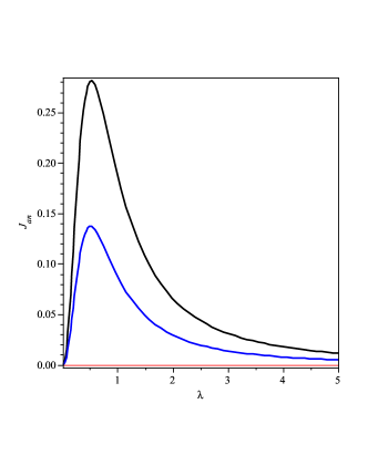
Figure 2: (Color online.) The normalized amplitude of the oscillating part of the current $J_{an}=$ $\mathcal{I}_{an}(P_{x},P_{y},v,\lambda)/\mathcal{I}_{c,n}(P_{x})$ as a function of the parameter $\lambda$ for $P_{x}=1$(black), and $P_{x}=2$(blue) with different scaling factors: $1\ast J_{an}(1)$ and $0.02\ast J_{an}(2)$ . Other parameters are: $P_{y}=5$, $v=1$.

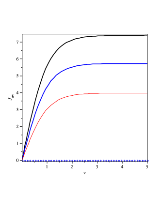
Figure 3: (Color online.) The same quantity as in Fig.2 as a function of the dimensionless voltage $v=eV/2T$ for $P_{x}=1$ (black), $P_{x}=2$ (blue) and $P_{x}=3$ (red). The scaling factors are: $30\ast J_{an}(1)$, $1\ast J_{an}(2)$ and $0.03\ast J_{an}(3)$.

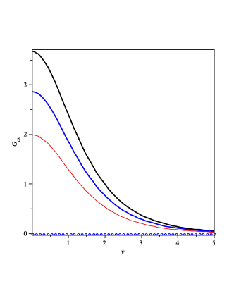
Figure 4: (Color online.) The normalized differential conductance $G_{an}$ vs the dimensionless voltage $v=eV/2T$ for the same parameters as in Fig.3.

The terms $m^{RR}(\zeta)$ and $m^{AA}(\zeta)$ contribute to the so-called regular part of the current $\delta\tilde{I}_{y}$

$$\delta\tilde{I}_{reg}=-\frac{1}{2}\int_{-\infty}^{\infty}d\zeta F_{V}(\zeta)[m^{RR}(\zeta)+m^{AA}(\zeta)]\text{.}$$ (38)

The anomalous current is given by

$$\delta\tilde{I}_{an}=2\int_{0}^{\infty}d\zeta F_{V}(\zeta)m^{RA}(\zeta)\text{.}$$ (39)

The integral in Eq.(38) can be transformed into the sum over Matsubara frequencies

$$\delta\tilde{I}_{reg}=-2\pi\text{Im}\sum_{n\geqslant 0}m(\zeta_{n}+2iv)$$ (40)

where $m(\zeta_{n})=m^{RR}(\epsilon_{n}/2T)$, $\epsilon_{n}=i\omega_{n}=T\zeta_{n}$, $\zeta_{n}=\pi(2n+1)$.

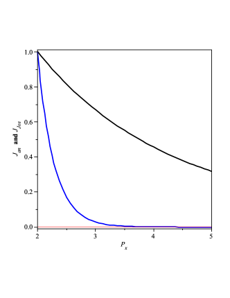
Figure 5: (Color online.) Comparison of the amplitude of oscillatory part of the current $J_{an}=0.23\ast\mathcal{I}_{an}(P_{x})/\mathcal{I}_{c,n}(2)$ and the Josephson critical current $J_{Jos}=\mathcal{I}_{c,n}(P_{x})/\mathcal{I}_{c,n}(2)$ in S - n - S junction as functions of the parameter $P_{x}$. One can see that the phase-coherent part of the current in N - F(n) - N circuit is much larger than the Josephson critical current $I_{c}$ in S - n - S junction.

We need to evaluate $m^{RA}(\epsilon)\equiv\langle\{\check{f}^{R}(y)\cdot\check{f}^{A}(y)\}_{0,0}\rangle$ as $m^{RR}(\epsilon)$ and $m^{AA}(\epsilon)$ can be found directly from it. The function $m^{RA}(\epsilon)$ can be obtained with the aid of Eq.(30). In particular, we find

$$m^{RA}(\zeta)=s^{RA}(\zeta)\exp(-(\theta_{x}^{R}+\theta_{x}^{A})\sum_{s=l,r}[C_{s}^{R}C_{s}^{A}+C_{s}^{R}C_{\bar{s}}^{A}\chi_{1}(\alpha,\beta)\cos\varphi],\textit{\ case 1}$$ (41)

and

$$m^{RA}(\zeta)=s^{RA}(\zeta)\exp(-(\theta_{x}^{R}+\theta_{x}^{A})\sum_{s=l,r}[a_{s}^{R}a_{s}^{A}+C_{s}^{R}C_{s}^{A}+\cos\varphi(a_{s}^{R}a_{\bar{s}}^{A}+\chi_{2}(\alpha,\beta)C_{s}^{R}C_{\bar{s}}^{A})],\textit{\ case 2}$$ (42)

with subscripts $s=l,r$ and $\bar{s}=r,l$. The coefficients $a$ and $C$ are also functions of $\zeta$. The function $m^{RR}(\epsilon)$ is obtained from Eqs.(41-42) by replacing $A\Rightarrow R$ and changing its sign. The angle-dependent function $\chi_{1,2}(\alpha,\beta)$ is then determined as

$$\chi(\alpha,\beta)=\Bigg{\{}\begin{array}[]{l}\chi_{1}(\alpha,\beta)\text{,}\quad\quad\quad\mathit{\quad\ \ \ \ \ \ \ \ \ \ }\text{{case 1}}\\ \chi_{1}(\alpha,\beta)+\cos\beta_{l}\cos\beta_{r}\text{,\ \ \ {case 2}}\end{array}$$ (43)

where $\chi_{1}(\alpha,\beta)=\cos(\alpha_{r}-\alpha_{l})\sin\beta_{l}\sin\beta_{r}$. The angles $\alpha_{l,r}$ and $\beta_{l,r}$ determine the orientation of the unit vector $\mathbf{n}$, see Eq.(18). The coefficients $s^{RA}(\zeta)$ and $s^{RR}(\zeta)$ are then equal to

$$s^{RA}(\epsilon) = \frac{\theta_{B}^{2}}{16|\theta_{y}^{R}(\zeta)|^{2}}\frac{\text{Im}[\theta_{y}(\zeta)\tanh\theta_{y}^{\ast}(\zeta)]}{\text{Re}\theta_{y}(\zeta)\text{Im}\theta_{y}^{\ast}(\zeta)}\text{,}$$ (44)

$$\text{ }s^{RR}(\epsilon_{n}) = \frac{\theta_{B}^{2}}{16\theta_{y}^{2}(\epsilon)\cosh^{2}\theta_{y}(\epsilon)}[\frac{\sinh(2\theta_{y}(\epsilon))}{2\theta_{y}(\epsilon)}-1]\text{,}$$ (45)

where $\theta_{B}=(\kappa_{B}^{2}w)L_{y}$, $\theta_{x,y}(\zeta)=P_{x,y}\sqrt{\zeta}$, $P_{x,y}=\sqrt{2T/E_{x,y}}$, $E_{x,y}=\{D/L^{2}\}_{x,y}$.

The most interesting parts of the current $\delta\tilde{I}=\delta\tilde{I}_{reg}+\delta\tilde{I}_{an}$ are the parts which depend on the phase $\varphi$ and angles $\{\alpha$, $\beta\}$. We represent them in the form

$$\delta\tilde{I}_{reg} = p_{i}\mathcal{I}_{reg}(v)\cos\varphi\chi_{i}(\alpha,\beta)\text{.}$$ (46)

$$\delta\tilde{I}_{an} = p_{i}\mathcal{I}_{an}(v)\cos\varphi\chi_{i}(\alpha,\beta)\text{.}$$ (47)

where the subindex $i=1,2$ stands for the cases 1,2. The amplitudes $\mathcal{I}_{reg}$, $\mathcal{I}_{an}$ are given by Eq.(57-62) in Appendix.

Eqs.(46-47) describe the oscillating part $\delta\tilde{I}$ of the current in the $y$-wire. It turns out that the function $\mathcal{I}_{reg}$,is much less than $\mathcal{I}_{an}$: $\mathcal{I}_{reg}$/$\mathcal{I}_{an}\lesssim 10^{-3}$ for $P_{x}=2$, $P_{y}=1$, and $\lambda_{1}=0.5$. One can show that, with increasing $P_{x}$, the anomalous part decays slower than the regular part (see Fig.5). Whereas the regular part decays with $P_{x}$ exponentially, $\mathcal{I}_{reg}\sim\exp[-2P_{x}(\pi^{2}+4v^{2})^{1/4}]$, the anomalous part $\mathcal{I}_{an}$ decreases in a power-law fashion. Earlier the slow decrease of anomalous contribution in space has been obtained in other problems Lempitsky98 ; TakayanVolkovPRL96 .

In Figs.2-5 we plot the dependence the normalized current $J_{an}=\mathcal{I}_{an}/\mathcal{I}_{J,n}$ and the differential conductance $G_{an}=(d\mathcal{I}_{an}(v)/dv)/\mathcal{I}_{J,n}$ vs different variables, i. e., vs the ”voltage $v$, the parameter $\lambda$. We plot Fig.2 for $\lambda=\lambda_{1}$; qualitatively similar form has the curve for$\lambda=\lambda_{2}$. The current $J_{an}(\lambda)$ increases from zero (no LRSTC in the absence of ferromagnetic films F_l,r with non-collinear magnetisations, i. e., at $\lambda=0$), reaches a maximum and then decreases to zero at large $\lambda$. As a function of the normalized voltage $v$ the current $J_{an}(v)$ increases to a constant value whereas the differential conductance $G_{an}$ drops to zero. The corresponding curves are shown in Figs.3 and 4 for different values of the parameter $P_{x}$; $P_{x}=1$, $2$ and $3$ from top to bottom.

V Josephson Current

In this section we calculate the Josephson current in an SF_l/F_st/F_rS  and SF_l/n/F_rS junctions using formulas for the condensate functions (see Eqs.(24-27)). Note that the obtained formulas for the Josephon current are also applicable to fully planar structures. The Josephson current in magnetic junctions was calculated in many theoretical papers. Ballistic regime was considered in Refs. HaltermanPRB15 ; RadovicPRB10 ; Mel'nikovPRL12 and diffusive case was analyzed in many papers for equilibrium BVEprl03 ; FominovPRB05 ; AnischPRB06 ; EschrigPRB07 ; BraudePRL07 ; HouzetPRB07 ; EschrigPRL08 ; EschrigPRL09 ; Kawabata10 ; GolubovPRL10 ; HaltermanSST16 and nonequilibrium cases Bobkov10 ; LinderHaltermanPRB14 ; Silaev19 ; Rahmonov19 . Since we assume that the length between superconductors $2L_{x}$ is larger than $\xi_{F}=\sqrt{D_{F}/E_{F}}$, we need to take into account only the LRSTC, i. e., the latter term in Eq.(24) and both components in Eq.(26). Substituting these components in Eq.(10), we obtain

$$I_{J}=I_{c}(\alpha,\beta)\sin\varphi\text{,}$$ (48)

where $\varphi$ is the phase difference and the critical current $I_{c}=I_{c}(\alpha,\beta)$ depends on orientation of the magnetization vectors $\mathbf{M}_{l,r}$ in the left and right layers F_l,r. This dependence has different forms in the cases 1 and 2.

The critical current $I_{c}$ is equal to

$$I_{c}(\alpha,\beta) = -(4\pi T/e)\sigma_{x}\chi_{1}(\alpha,\beta)\sum_{\omega}|C_{r}C_{l}|\kappa_{\omega}\exp(-2\kappa_{\omega}L_{x}),\text{{Case 1}}$$ (49)

$$I_{c}(\alpha,\beta) = (4\pi T/e)\sigma_{x}\sum_{\omega}[a_{l}a_{r}-\chi_{2}(\alpha,\beta)C_{r}C_{l}]\kappa_{\omega}\exp(-2\kappa_{\omega}L),\text{{Case 2}}$$ (50)

where the coefficients $C_{l,r}$ are defined in Eqs.(25) and the function $\chi(\alpha,\beta)$ in Eq.(43). The coefficients $a_{l,r}$ and $C_{l,r}$ are given in Eq.(27).

Note, at $\beta_{l}=\beta_{r}=\pi/2$, the sign of the critical current $I_{c}$ is determined by the difference $(\alpha_{r}-\alpha_{l})$. If this difference is equal to $\pi$, that is, the vector $\mathbf{n}_{\perp}$ rotates by $\pi$ over the length $2L$, then $I_{c}$ is positive. If the rotation angle is zero, the current $I_{c}$ becomes negative. The first case can be called topological since the winding number of the vector $\mathbf{n}_{\perp}$ in the first case is $var\{angle(\mathbf{n}_{\perp})\}/\pi=1$, while in the second case $var\{angle(\mathbf{n}_{\perp})\}/\pi=0$. The sign change of the current $I_{c}$ can occur not only in magnetic Josephson junctions, but also in multiterminal structures with a non-equilibrium distribution function VolkovPRL95 ; ZaikinPRL98 ; Yip98 ; Bobkov10 ; Bobkov12 . In other words, the SF_l-F-F_rS circuit models a ferromagnetic wire with two domain walls. The topological configuration with $(\alpha_{l}-\alpha_{r})=\pi$ corresponds to a positive $I_{c}$ (the magnetization vector $\mathbf{M}$ rotates clockwise or counter clockwise) that the critical current $I_{c}(\alpha)$ is positive if the difference $(\alpha_{l}-\alpha_{r})=\pi$. In a non-topological case when the vector $\mathbf{M}$ rotates first by $\pi/2$ from $\alpha_{l}=0$ at F_l and then returns to $\alpha_{r}=0$, the critical current in the last case is negative.

The first term in Eq.(50) is due to the singlet component. The second term that changes sign by varying the angles $\alpha$ is caused by the triplet component. If the parameter $\kappa_{l,r}$ is small compared to $\kappa_{\omega}$, i. e. $\kappa_{l,r}\xi_{T}\ll 1$, then the first term in square brackets dominates and the critical current is positive. In the opposite limit, $\kappa_{l,r}\xi_{T}\gg 1$, the second term in Eq.(50) is larger than the first one and the sign of $I_{c}$ depends on orientations of the vector $\mathbf{M}_{l,r}$.

In analogy with Eqs.(46-47), the angle-dependent part of the critical current $I_{c}(\alpha,\beta)$ can be written as

$$\tilde{I}_{c}(\alpha,\beta) = p_{J}\mathcal{I}_{Jos}\chi(\alpha,\beta)\text{,}$$ (51)

$$\mathcal{I}_{Jos} = 2\pi\sum_{n\geqslant 0}|C(\zeta_{n})|^{2}\sqrt{\zeta_{n}}\exp(-2P_{x}\sqrt{\zeta_{n}})$$ (52)

where $p_{J1,2}$ are given in Appendix (Eqs.(63)).

In order to compare the formulas for the currents $I_{an}$, $I_{Jos}$, it is useful to write down the formula for the critical current $I_{c,n}$ in an S - n - S junction. The formula for $I_{c,n}$ can be directly found from Eq.(50) by setting $C=0$

$$I_{c,n}=2\pi(\frac{\kappa_{b}}{\kappa_{T}})^{2}\sum\frac{\exp(-2P_{x}\sqrt{\zeta_{n}})}{\sqrt{\zeta_{n}}}\frac{\tilde{\Delta}^{2}}{\tilde{\Delta}^{2}+\zeta_{n}^{2}}\text{.}$$ (53)

where $\tilde{\Delta}=\Delta/(2T)$.

At $\varphi=0$, the Josephson current $I_{J}$ turns to zero for any angles $\alpha$ and $\beta$. In the terminology of Ref.MoorVE15 , the obtained result corresponds to the nematic case in contrast to the ferromagnetic one when the Josephson current $I_{J}\neq 0$ even for $\varphi=0$. The phase-current relation in the latter case has the form $I_{J}=I_{c}\sin(\varphi+\psi)$, where $\psi$ is an angle dependent constant. The unusual phase dependence of the critical Josephson current may arise in the presence of spin-orbit interaction Krive05 ; Buzdin08 ; Balseiro08 ; Nazarov14 ; TokatlyPRB15 ; Silaev17 , in the case of spin filters BuzdinAPL20 ; MoorVE15 or in S/AF/S Josephson junctions with antiferromagnetic (AF) layer RabinovichPRR19 .

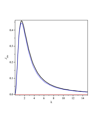
Figure 6: (Color online.) The ratio of the critical Josephson current in the system under consideration and in a S - n - S Josephson junction, $J_{Jos}=$ $\mathcal{I}_{Jos}(P_{x},\lambda)/\mathcal{I}_{c,n}(P_{x})$, with equal S/n or S/F_l,r interface transparency as a function of the parameter $\lambda$ for $P_{x}=1$ (black) and $P_{x}=2$ (blue).

In the considered nematic case, the angle dependence of the current $I_{c}$ is determined by the function $\chi(\alpha,\beta)$. For $\beta_{l}=\beta_{r}=\pi/2$ and $\alpha_{l}=-\alpha_{r}=\alpha$, the angle dependence of $I_{c}$, Eq.(53), coincides with that obtained by Braude and Nazarov (see Eq.(8) for the critical current $I_{c}=I_{\uparrow}+I_{\downarrow}$ in Ref.BraudePRL07 ). However, the amplitudes of $I_{c}$ are different because the models considered here and in Ref.BraudePRL07 are different (a weak PE, a long JJ in our model and a strong PE and a short JJ in Ref.BraudePRL07 ). For $\alpha_{l}=\alpha_{r}$ the angle dependence of the critical current $I_{c}$, Eq.(53), is the same as obtained by Buzdin and Houzet HouzetPRB07 for a three magnetic layer SF_lFF_rS Josephson junction. This model has been analysed recently by Houzet and Birge in more detail Birge19 (see also Birge20 ). Similar angle dependence of the Josephson critical current was obtained, mostly numerically, in Ref.HaltermanPRB14 .

Figure 7: (Color online.) The dependence of the critical current on the field $h$.

In Fig.6 we show the normalized critical current $J_{c}=\mathcal{I}_{c}(\lambda)/\mathcal{I}_{c,n}$ as a function of $\lambda$. One can see that the critical current reaches a maximum value at $\lambda\sim 1$ and decreases to zero at large $\lambda$.

V.1 Negative Josephson Current and Paramagnetic Response

In this section we discuss the analogy between negative critical Josephson current $I_{c}$ and a paramagnetic response of a superconducting system to an external magnetic field. As we mentioned before, the negative $I_{c}$ may arise in a magnetic S-F-S Josephson junctions and in multiterminal S-n-S Josephson junctions with a nonequilibrium distribution function $\hat{n}(\epsilon)$. The negative $I_{c}$ in magnetic JJs has been predicted in Refs.Bulaev77 ; BuzdinKup90 and observed in Refs.RyazanovPRL01 ; RyazanovPRL06 . In a recent paper LinderBelzigPRL20 , the possibility of a paramagnetic response of S-n bilayer with a nonequilibrium distribution function was analyzed . Here we point out the close analogy between negative $I_{c}$ and paramagnetic response. We show that the response of a JJ with negative $I_{c}$ to external fields (ac electric or magnetic) is paramagnetic regardless of the mechanism of negative critical current. Indeed, it is well known that at low temperatures, a JJ in an electric circuit plays a role of an inductance $\mathcal{L}$. For small variation $\delta\varphi=\varphi-\varphi_{0}$ and $I_{J},$ Eq.(48) can be written

$$\partial I_{J}/\partial t\cong I_{c}\partial(2\delta\varphi)/\partial t\cos\varphi_{0}=I_{c}\frac{2eV}{\hbar}\text{.}$$ (54)

As follows from this equation, $\mathcal{L}=I_{c}\hbar/(2e)\cos\varphi_{0}$. Thus, at a fixed $\varphi_{0}$ the inductance $\mathcal{L}$ changes sign if $I_{c}$ becomes negative. On the other hand, the London equation yields

$$\partial I_{J}/\partial t = -\Lambda\partial A/\partial t=c\Lambda E=$$ (55)

$$= c(\Lambda/l_{ch})V\text{.}$$ (56)

where $l_{ch}$ is a characteristic length which is determined by a concrete type of  a system. The effective inductance is $\mathcal{L}=l_{ch}/(c\Lambda)$. The positive coefficient $\Lambda$ corresponds to a diamagnetic response while negative $\Lambda$ describes a paramagnetic response. The negative inductance $\mathcal{L}$ means a paramagnetic response of a JJ which has a negative $I_{c}$.

Figure 8: (Color online.) The dependence of the integral $J$ on the ratio $R=P_{y}/P_{y}$.

VI Conclusions

We have studied propagation of the LRSTC in a magnetic Andreev interferometer. The LRSTC is created by two thin ferromagnetic layers F_l,r deposited on the superconductors S. For the propagation of the LRSTC it does not matter whether the wires connecting the normal metal reservoirs N or superconducting reservoirs S are made of normal (n) or magnetic (F) metals. The magnetic layers F_l,r have magnetisations $M_{l,r}$ which are characterized by the angles $(\alpha)_{l,r}$ in the spin space. The oscillating part of the dissipative current between the N reservoirs $I_{osc}=I_{V}\chi(\alpha,\beta)\cos\varphi$ has the same angle dependence as the Josephson current between the S reservoirs $I_{J}=I_{c0}\chi(\alpha)\sin\varphi$. However, the current $I_{osc}$ decreases with increasing temperature $T$ or the length $L_{x}$ much slower than the critical current $I_{c0}$ (see Fig.6). In the first case the decrease follows the power law behavior, while in the second case the decrease is exponential: $I_{c0}\sim\exp(-2L_{x}/\xi(T))$. The critical current $I_{c}=I_{c0}\chi(\alpha,\beta)$ has different signs in topological JJ’s ($\alpha_{r}-\alpha_{l}=\pi$) and in non-topological ones ($\alpha_{r}-\alpha_{l}=0$). At certain angles, the Josephson and phase-dependent dissipative currents turn to zero, for example, for angles $\alpha_{r}-\alpha_{l}=(\pi/2)(2n+1)$ and $\beta_{r,l}=\pi/2$. Note that we assumed that the proximity effect is weak. This is true if the parameters $\kappa_{b,B}/\kappa_{\omega}\ll 1$. However the obtained results remain qualitatively valid if this ratio is of the order of 1.

In the language of Ref.MoorVE15 , the obtained current-phase dependence, $I_{J}=I_{c}\sin\varphi$, corresponds to a nematic case contrary to a ferromagnetic case, $I_{J}=I_{c}\sin(\varphi+\psi)$, that is, the Josephson current is equal to zero for the phase difference $\varphi=0$. Therefore, it is of interest experimentally to investigate the angle and phase dependence of the currents $I_{J}$ and $I_{osc}$. The obtained results for the Josephson current $I_{J}$ are valid not only for the JJ shown in Fig.1, but also for a planar geometry used in Ref.BirgePRL10 ; BirgePRL16 . Note also that the measurements of the $I_{osc}$ in Andreev interferometers provides an additional possibility to study the propagation of the LRSTC in magnetic superconducting structures.

VII Acknowledgements

The author thanks Ilya M. Eremin for careful reading of the manuscript and acknowledge support from the Deutsche Forschungsgemeinschaft Priority Program SPP2137, Skyrmionics, under Grant No. ER 463/10.

VIII Appendix

The formulas for the amplitudes $\mathcal{I}_{reg}$, $\mathcal{I}_{an}$ can be readily obtained from Eqs.(39-40). We find

$$\mathcal{I}_{reg}(v) = \frac{\pi}{4}\text{Im}\sum_{n\geqslant 0}\{\frac{c_{reg}(\zeta_{n})\exp(-2\theta_{x}(\zeta_{n}))}{(\zeta_{n}+2iv)\cosh^{2}\theta_{y}(\zeta_{n})}[\frac{\sinh(2\theta_{y}(\zeta_{n}))}{2\theta_{y}(\zeta_{n})}-1]\}$$ (57)

$$\mathcal{I}_{an}(v) = -\frac{1}{8}\frac{\sinh(2v)}{P_{y}}\int_{0}^{\infty}\frac{c_{an}(\zeta)d\zeta}{\zeta^{3/2}}\frac{\text{Im}[(1-i)\tanh(P_{y}(1+i)\sqrt{\zeta})]}{\cosh(\zeta+v)\cosh(\zeta-v)}\}\exp(-2P_{x}\sqrt{\zeta})\text{,}$$ (58)

where $\theta_{x,y}(\zeta_{n})=P_{x,y}\sqrt{\zeta_{n}+2iv}$. The functions $j_{reg,an}$ are given by equations

$$c_{reg}(\zeta_{n}) = -\frac{\lambda_{1,2}^{2}}{[\lambda_{1,2}^{2}+\sqrt{\zeta_{n}+2iv}]^{2}}(F_{S}^{R})^{2},$$ (60)

$$c_{an}(\zeta) = \frac{\lambda_{1,2}^{2}}{(\lambda_{1,2}^{2}+\sqrt{\zeta})^{2}+\zeta}F_{S}^{R}F_{S}^{A}.$$ (61)

and the constants $\lambda_{1,2}$ are equal to: $\lambda_{1}\mathcal{=}\kappa_{l}/\sqrt{\kappa_{F}\kappa_{T}}$, $\lambda_{2}\mathcal{=}\kappa_{l}/\kappa_{T}$.

The constants $p_{i}$ and $p_{J1,2}$are defined as follows

$$p_{1} \mathcal{=} \frac{1}{2}(\frac{\kappa_{B}\kappa_{b}}{\kappa_{T}^{2}})^{2}(\frac{\kappa_{T}}{\kappa_{F}})\text{, }p_{2}\mathcal{=}\frac{1}{2}(\frac{\kappa_{B}\kappa_{b}}{\kappa_{T}^{2}})^{2}\text{,}$$ (62)

$$p_{J1} \mathcal{=} (\frac{\kappa_{b}}{\kappa_{T}})^{2}(\frac{\kappa_{T}}{\kappa_{F}})\text{, }p_{J2}\mathcal{=}(\frac{\kappa_{b}}{\kappa_{T}})^{2}\text{.}$$ (63)

We also write the expression of the critical current $\tilde{I}_{c}=I_{c}(..)$ of a S - n - S Josephson junction with the same S/n interface penetrability as in the considered structure. This quantity can serve as a reference scale of the current

$$\delta\tilde{I}_{c,n}=p_{n}\mathcal{I}_{c,n}\sin\varphi\text{.}$$ (64)

where $p_{n}=(\kappa_{b}/\kappa_{T})^{2}$ and the function $\mathcal{I}_{n}$ is

$$\mathcal{I}_{c,n}=2\pi\sum_{n\geqslant 0}\frac{\exp(-2P_{x}\sqrt{\zeta_{n}})}{\sqrt{\zeta_{n}}}\text{.}$$ (65)

with $\zeta_{n}=\pi(2n+1)$.

References

• (1) Kulik, I. O., and I. K. Yanson, 1970, The Josephson Effect in Superconducting Tunneling Structures Nauka, Moscow; John Wiley & Sons, Incorporated, 1972.
• (2) K. K. Likharev, Rev. Mod. Phys. 51, 101 (1979).
• (3) A. Barone and G. Paterno, in Physics and Applications of the Josephson Effect, (Wiley, New York, 1982), pp. 1–24.
• (4) B. D.Β Josephson, Physics Lett. 1, 251 (1962)
• (5) A. A. Golubov, M. Yu. Kupriyanov, and E. Il’ichev, Rev. Mod. Phys. 76, 411 (2004)
• (6) A. I. Buzdin, Rev. Mod. Phys. 77, 935 (2005).
• (7) L. N. Bulaevskii, V. V. Kuzii, and A. A. Sobyanin, Pis’ma Zh. Eksp. Teor. Fiz. 25, 314 (1977) [JETP Lett. 25, 290 1977] .
• (8) A. I.Β Buzdin, L. N. Bulaevskii, and S. V. Panjukov, , Pis’ma Zh. Eksp. Teor. Fiz. 35, 147 (1982); JETP Lett. 35, 20 (1982).
• (9) Buzdin, A. I., and M. Y. Kupriyanov, Pis’ma Zh. Eksp. Teor. Fiz. 52, 1089 ( 1990) [JETP Lett. 52, 487 1990].
• (10) A. I. Buzdin and M. Y. Kuprianov, Pis’ma Zh. Eksp. Teor. Fiz. 53, 308 (1991) [JETP Lett. 53, 321 (1991)].
• (11) V. V. Ryazanov, , V. A. Oboznov, A. Yu. Rusanov, A. V. Veretennikov, A. A. Golubov, and J. Aarts, Phys. Rev. Lett. 86, 2427 (2001).
• (12) V. A. Oboznov, V. V. Bol’ginov, A. K. Feofanov, V. V. Ryazanov, and A. I. Buzdin, Phys. Rev. Lett. 96, 197003 (2006).
• (13) T. Kontos, M. Aprili, J. Lesueur, F.Genet, B. Stephanidis, and R. Boursier, Phys. Rev. Lett. 89, 137007 (2002).
• (14) H. Sellier, C. Baraduc, F. Lefloch, and R. Calemczuk, Phys. Rev. B 68, 054531 (2003).
• (15) M. Weides, M. Kemmler, E. Goldobin, D. Koelle, R. Kleiner, H. Kohlstedt, and A. Buzdin, Appl. Phys. Lett. 89, 122511 (2006).
• (16) F. S. Bergeret, A. F. Volkov, and K. B. Efetov, Rev. Mod. Phys. 77, 1321 (2005).
• (17) M. Eschrig, Phys. Today 64(1), 43 (2011); Rep. Prog. Phys. 78, 104501 (2015).
• (18) J. Linder and J. W. A. Robinson, Nature Physics 11, 307-315 (2015).
• (19) J. Linder, A. V. Balatsky, Rev. Mod. Phys. 91, 045005 (2019).
• (20) F. S. Bergeret, A. F. Volkov, and K. B. Efetov, Phys. Rev. Lett. 86, 3140 (2001).
• (21) A. Kadigrobov, R. I. Shekhter, and M. Jonson, Europhys. Lett. 54, 394 (2001).
• (22) The idea similar to that presented in Ref.BVEprl01 was discussed a little later in Ref.Kadigr01 . The authors of Ref.BVEprl01 considered a diffusive case using the Usadel equation. The width of the domain wall $d_{DW}$ in the ferromagnet was assumed to be larger than the mean free path $l$. The authors of Ref. Kadigr01 considered the case when $d_{DW}\lesssim l$. However they could not find the appropriate correct solution for the Eilenberger equation. This solution for the case of a narrow domain wall has been found in Ref.VolkovEfetovPRB08 .
• (23) A. F. Volkov, and K. B. Efetov, Phys. Rev. B 78, 024519 (2008).
• (24) R.S. Keizer, S.T.B. Goennenwein, T.M. Klapwijk, G. Miao, G. Xiao, and A. Gupta, Nature (London) 439, 825 (2006).
• (25) H. Sosnin, H. Cho, V.T. Petrashov, and A.F. Volkov, Phys. Rev. Lett. 96, 157002 (2006).
• (26) J.W.A. Robinson, J.D.S. Witt and M.G. Blamire, Science 329, 59 (2010).
• (27) T.S. Khaire, M.A. Khasawneh, W.P. Pratt Jr. and N.O. Birge, Phys. Rev. Lett. 104, 137002 (2010);
• (28) C. Klose et al, Phys. Rev. Lett. 108, 127002 (2012); W. Martinez, W. P. Pratt, Jr., N. O. Birge, Phys. Rev. Lett. 116, 077001 (2016).
• (29) D. Sprungmann, K. Westerholt, H. Zabel, M. Weides and H. Kohlstedt, Phys. Rev. B 82, 060505 (2010).
• (30) M. S. Anwar, F. Czeschka, M. Hesselberth, M. Porcu, and J. Aarts, Phys. Rev. B 82, 100501 (2010).
• (31) M. S. Kalenkov, A. D. Zaikin, and V. T. Petrashov, Phys. Rev. Lett. 107, 087003 (2011).
• (32) J. W. A. Robinson, G. B. HalΓ‘sz, A. I. Buzdin, and M. G. Blamire, Phys. Rev. Lett. 104, 207001 (2010). M. G. Blamire and J. W. A. Robinson, J. Phys. Condens. Matter 26, 453201 (2014).
• (33) D. Massarotti, N. Banerjee, R. Caruso, G. Rotoli, M. G. Blamire, and F. Tafuri, Phys. Rev. B 98, 144516 (2018).
• (34) B. M. Niedzielski, T.J. Bertus, J. A. Glick, R. Loloee, W. P. Pratt Jr., N. O. Birge, Phys. Rev. B 97, 024517 (2018).
• (35) F. S. Bergeret, A. F. Volkov, and K. B. Efetov, Phys. Rev. Lett. 90, 117006 (2003).
• (36) A. F. Volkov, A. Anishchanka, K. B Efetov, Phys. Rev. B 73, 104412 (2006).
• (37) T. Lofwander, T. Champel, M. Eschrig, Phys. Rev. B 75, 014512 (2007).
• (38) T. Champel, T. LΓΆfwander, M. Eschrig, Phys. Rev. Lett. 100, 077003 (2008).
• (39) Luka Trifunovic and Zoran RadoviΔ‡, Phys. Rev. B 82, 020505(R) (2010).
• (40) A. S. Mel’nikov, A. V. Samokhvalov, S. M. Kuznetsova, and A. I. Buzdin, Phys. Rev. Lett. 109, 237006 (2012).
• (41) Shiro Kawabata, Yasuhiro Asano, Yukio Tanaka, Satoshi Kashiwaya, Physica E 42, 1010 (2010).
• (42) S. Kawabata, Y. Asano, Y. Tanaka, A. A. Golubov, S. Kashiwaya, Phys. Rev. Lett. 104, 117002 (2010).
• (43) M. Alidoust, K. Halterman, Phys. Rev. B 89, 195111 (2014).
• (44) Klaus Halterman, Oriol T. Valls, Chien-Te Wu, Phys. Rev. B 92, 174516 (2015).
• (45) K. Halterman, M. Alidoust, Supercond. Sci. Technol. 29, 055007 (2016)
• (46) N. O. Birge and M.Β Houzet, arXiv:191001230.
• (47) H. G. Ahmad, R. Caruso, A. Pal, G. Rotoli, G. P. Pepe, M. G. Blamire, F. Tafuri, D. Massarotti, Phys. Rev. Applied 13, 014017 (2020)
• (48) V. Aguilar, D. Korucu, J. A. Glick, R. Loloee, W. P. Pratt Jr., N. O. Birge, arXiv:2005.066
• (49) Sachio Komori, et al., arXiv:2006.16654.
• (50) R. Caruso, et al., Phys. Rev. Lett. 122, 047002 (2019).
• (51) V. T. Petrashov, V. N. Antonov, P. Delsing, and T. Claeson, JETP Lett.60,606 (1994).
• (52) A. Dimoulas, J. P. Heida, B. J. v. Wees, T. M. Klapwijk, W. v. d. Graaf, and G. Borghs, Phys. Rev. Lett. 74, 602 (1995).
• (53) H. Courtois, Ph. Gandit, D. Mailly, and B. Pannettier, Phys. Rev. Lett.76,130 (1996);
• (54) P. Charlat, H. Courtois, Ph. Gandit, D. Mailly, A. F. Volkov, and B. Pannettier, Phys. Rev. Lett.77, 4950 (1996).
• (55) A. F. Volkov and H. Takayanagi, Phys. Rev. Lett. 76, 4026 (1996.)
• (56) V. T. Petrashov, I. A. Sosnin, I. Cox, A. Parsons, and C. Troadec, Phys. Rev. Lett. 83, 3281 (1999)
• (57) R. Shaikhaidarov, A. F. Volkov, H. Takayanagi, V. T. Petrashov, P. Delsing, Phys. Rev. B 62, R14649(R) (2000).
• (58) V. T. Petrashov, K. G. Chua, K. M. Marshall, R. Sh. Shaikhaidarov, J. T. Nicholls, Phys. Rev. Lett. 95, 147001 (2005).
• (59) E. Kandelaki, A. F. Volkov, K. B. Efetov, and V. T. Petrashov, Phys. Rev. B 82, 024502 (2010).
• (60) A. V. Galaktionov, A. D. Zaikin, L. S Kuzmin, Phys. Rev. B 85, 224523 (2012) .
• (61) F. Vischi, M. Carrega, E. Strambini, S. D’Ambrosio, F. S. Bergeret, Yu. V. Nazarov, F. Giazotto, Phys. Rev. B 95, 054504 (2017).
• (62) P. E. Dolgirev, M. S. Kalenkov, A. E. Tarkhov, A. D. Zaikin, Phys. Rev. B 100, 054511 (2019).
• (63) L. F. Chang and P. F. Bagwell, Phys. Rev. B55, 12678(1997).
• (64) V. Bezuglyi, V. S. Shumeiko, G. Wendin, Phys. Rev. B v.68, 134506 (2003).
• (65) A. F. Volkov, Phys. Rev. Lett. 74, 4730 (1995).
• (66) F. K. Wilhelm, G. SchΓΆn, and A. D. Zaikin, Phys. Rev. Lett. 81,1682 (1998).
• (67) S. K. Yip, Phys. Rev. B58, 5803 (1998).
• (68) I. V. Bobkova, A. M. Bobkov, Phys. Rev. Lett. 108, 197002 (2012).
• (69) I. V. Bobkova, A. M. Bobkov, Phys. Rev. B 82, 024515 (2010); ibid 84, 054533 (2011)
• (70) J. J. A. Baselmans, B. J. van Wees, and T. M. Klapwijk, Phys. Rev. B 65, 224513 (2002).
• (71) R. S. Keizer, S. T. B. Goennenwein, T. M. Klapwijk, G. Miao, G. Xiao, and A. Gupta, Nature 439, 825 (2006).
• (72) A. G. Mal’shukov, Phys. Rev. B 97, 064515 (2018).
• (73) D. A. Ivanov, Ya. V. Fominov, M. A. Skvortsov, P. M. Ostrovsky, Phys. Rev. B 80, 134501 (2009).
• (74) A. I. Larkin, and Y. N. Ovchinnikov, 1984, Nonequilibrium Superconductivity Elsevier, Amsterdam , p. 530.
• (75) A. Volkov, A. Zaitsev, and T. Klapwijk, Physica C (Amsterdam) 210, 21 (1993).
• (76) A. V. Zaitsev, A. F. Volkov, S. W. D. Bailey, and C. J. Lambert, Phys. Rev. B 60, 3559 (1999).
• (77) W. Belzig, F.K.Wilhelm, C. Bruder, G. SchΒ¨on, andA.D. Zaikin, Superlatt. Microstruct. 25, 1251 (1999).
• (78) N. Kopnin, Theory of Nonequilibrium Superconductivity, (Oxford Science, London, 2001).
• (79) A.V. Zaitsev, Sov. Phys. JETP 59 (1984) 863.
• (80) M. Yu. Kupriyanov and V. F. Lukichev, Zh. Eksp. Teor. Fiz. 94, 139 (1988) [Sov. Phys. JETP 67, 1163 (1988)]
• (81) M. A. Silaev, I. V. Tokatly, F. S. Bergeret, Phys. Rev. B 95, 184508 (2017).
• (82) D. S. Rabinovich, I. V. Bobkova, A. M. Bobkov, M. A. Silaev, Phys. Rev. Lett. 123, 207001 (2019)
• (83) A. V. Zaitsev, Physica B203, 274 (1994).
• (84) Yu. V. Nazarov and T. H. Stoof, Phys. Rev. Lett76, 823 (1996).
• (85) A. A. Goluov, F. K. Wilhelm, A. D. Zaikin, Phys. Rev.B55, 1123 (1997).
• (86) S.V. Lempitsky Sov. Phys. JETP 57, 910(1983)
• (87) A. Moor, A. F. Volkov, K. B. Efetov, Phys. Rev. B 93, 104525 (2016).
• (88) A. F. Volkov, Y. V. Fominov, and K. B. Efetov, Phys. Rev. B 72, 184504 (2005).
• (89) V. Braude, Yu. V. Nazarov, Phys. Rev. Lett. 98, 077003 (2007).
• (90) M. Houzet and A. I. Buzdin, Phys. Rev. B 76, 060504 (2007).
• (91) R. Grein, M. Eschrig, G. Metalidis, Gerd SchΓΆn, Phys. Rev. Lett. 102, 227005 (2009) .
• (92) J. Linder, K. Halterman, Phys. Rev. B. 90, 104502 (2014).
• (93) Yu. M. Shukrinov, I. R. Rahmonov, and K. Sengupta, Phys. Rev. B 99, 224513 (2019).
• (94) I. V. Krive, A. M. Kadigrobov, R. I. Shekhter, and M.Jonson, Phys. Rev. B71, 214516 (2005).
• (95) A. Buzdin, Phys. Rev. Lett.101, 107005 (2008).
• (96) T. Yokoyama, M. Eto, Y. V. Nazarov, Phys. Rev. B89,195407 (2014).
• (97) F. Konschelle, I. V. Tokatly, and F. S. Bergeret, Phys. Rev. B 92, 125443 (2015).
• (98) A. A. Reynoso, G. Usaj, C. A. Balseiro, D. Feinberg, andM. Avignon, Phys. Rev. Lett.101, 107001 (2008).
• (99) J. A. Ouassou, W. Belzig, J. Linder, Phys. Rev. Lett. 124, 047001 (2020).
• (100) D. S. Rabinovich, I. V. Bobkova, A. M. Bobkov, Phys. Rev. Research 1, 033095 (2019).
• (101) A. Moor, A. F. Volkov, K. B. Efetov, Phys. Rev. B 92,180506(R) (2015).
• (102) S. Mironov, H. Meng, A. Buzdin, Appl. Phys. Lett. 116, 162601 (2020).