Black-box Adversarial Example Generation with Normalizing Flows

Abstract

Deep neural network classifiers suffer from adversarial vulnerability: well-crafted, unnoticeable changes to the input data can affect the classifier decision. In this regard, the study of powerful adversarial attacks can help shed light on sources of this malicious behavior. In this paper, we propose a novel black-box adversarial attack using normalizing flows. We show how an adversary can be found by searching over a pre-trained flow-based model base distribution. This way, we can generate adversaries that resemble the original data closely as the perturbations are in the shape of the data. We then demonstrate the competitive performance of the proposed approach against well-known black-box adversarial attack methods.

1 Introduction

Deep neural network (DNN) classifiers have been successfully applied to many object recognition tasks. However, Szegedy et al. (2014) pointed out that even the slightest intentional changes to a DNN input, widely known as adversarial attacks, can change the classifier decision. This observation is peculiar as those changes are tiny and can barely affect a human’s judgment about the object class. Since their emergence, many adversarial attack methods have been devised. These studies are often helpful in recognizing sources of this misbehavior, which ultimately can lead to more robust DNN classifiers.

There are many attributes by which adversarial attacks can be categorized (Yuan et al., 2019). Perhaps the most famous one is with respect to the adversary’s knowledge about the target DNN. In this sense, threat models are divided into white- and black-box attacks. In white-box attacks, it is assumed that the adversary has full access to the internal weights of the target DNN, and can leverage this knowledge in generating adversarial examples by using the DNN gradients. In contrast, black-box adversarial attacks are assumed to have access to solely the input and output of a classifier. As a result, they have to utilize this limited capacity in order to construct their adversarial examples.

There has been some research on the use of generative models in the construction of adversarial examples, for instance,  Baluja & Fischer (2018); Xiao et al. (2018); Song et al. (2018); Wang & Yu (2019). These works are mostly concerned with training a generative model on a target network so that the samples generated by them are adversarial. To this end, they often require taking the gradient of the target network, and hence, are mostly suitable for white-box settings. To adapt themselves to the black-box scenario, they often replace the target network with a substitute version. Thus, the performance of such approaches heavily depends on the resemblance of the target network to the substitute one. Moreover, for various types of defenses, such methods often require re-training their generator on a different substitute network.

In this paper, we propose using pre-trained flow-based models to generate adversarial attacks for the black-box setting. We first formulate the problem of adversarial example generation. Then, we show how searching over the base distribution of a pre-trained normalizing flow can be related to generating adversaries. Finally, we show the effectiveness of the proposed method in attacking vanilla and defended models. We see that the perturbations generated by our method follow the shape of the data closely. However, this is generally not the case for other existing methods, as they often look like an additive noise.

To the best of our knowledge, this is the first work that exploits normalizing flows to generate adversarial examples. Through the experimental results, we see how this method can be used to make adversarial perturbations less noticeable. We hope our work can be a stepping stone into modeling adversaries using exact likelihood approaches with their ability to model the data distribution closely. Hopefully, such works can lead to the statistical treatment of DNNs’ adversarial vulnerability.

2 Background

2.1 Normalizing Flows

Normalizing flows (Tabak & Turner, 2013; Dinh et al., 2015; Rezende & Mohamed, 2015) are a relatively novel family of generative models. They use invertible neural networks (INN) to transform a simple density into data distribution. To this end, they exploit the change of variables theorem. In particular, assume that ${\mathbf{Z}\in\mathbb{R}^{d}}$ denote an arbitrary random vector from a uniform or standard normal distribution. If we construct a new random vector ${\mathbf{X}\in\mathbb{R}^{d}}$ by applying a differentiable INN ${\mathbf{f}(\cdot):\mathbb{R}^{d}\rightarrow\mathbb{R}^{d}}$ to ${\mathbf{Z}}$, then the relationship between their corresponding densities can be written as

$$p(\mathbf{x})=p(\mathbf{z})\left|\mathrm{det}\Big{(}\dfrac{\partial\mathbf{f}}{\partial\mathbf{z}}\Big{)}\right|^{-1}.$$ (1)

The multiplicative term on the RHS is known as the Jacobian determinant. This term accounts for normalizing the base distribution ${p(\mathbf{z})}$ such that the density ${p(\mathbf{x})}$ represents the data distribution. To make modeling of high-dimensional data feasible, the Jacobian determinant must be computed efficiently. Otherwise, this calculation can hinder the application of such models to high-dimensional data as the cost of computing the determinant grows cubically with the data dimension. Once set, we can use maximum likelihood to fit the flow-based model of Eq. (1) to data observations. This fitting is done using numerical optimization methods such as Adam (Kingma & Ba, 2015).

One of the earliest INN designs for flow-based modeling is Real NVP (Dinh et al., 2017). This network uses affine transformations in conjunction with ordinary neural networks such as ResNets (He et al., 2016) to construct a normalizing flow. In this paper, we use a reformulation of Real NVP (Dinh et al., 2017) introduced by Ardizzone et al. (2019). This transformation is defined by stacking two consecutive layers of ordinary Real NVP together

$$\mathbf{x}_{1} =\mathbf{z}_{1}\odot\exp\big{(}\mathbf{s}_{1}({\mathbf{z}_{2}})\big{)}+\mathbf{t}_{1}({\mathbf{z}_{2}})$$

$$\mathbf{x}_{2} =\mathbf{z}_{2}\odot\exp\big{(}\mathbf{s}_{2}({\mathbf{x}_{1}})\big{)}+\mathbf{t}_{2}({\mathbf{x}_{1}}).$$ (2)

Here, ${\mathbf{s}_{1,2}(\cdot)}$ and ${\mathbf{t}_{1,2}(\cdot)}$ represent the scaling and translation functions, and they are implemented using ordinary neural networks as they are not required to be invertible. For more information about flow-based models and architectures, we refer the interested reader to Kobyzev et al. (2019); Papamakarios et al. (2019).

2.2 Adversarial Example Generation

Let $\mathcal{C}(\cdot)$ denote a DNN classifier. Assume that this network is defined so that it takes an image $\mathbf{x}$ as its input, and outputs a vector whose $y$-th element indicates the probability of the input belonging to class $y$. Now, we can solve the following optimization problem to find an adversarial example for $\mathbf{x}$

$${\mathbf{x}}_{adv}=\operatorname*{arg\,min}_{\left\lVert\mathbf{x}^{\prime}-\mathbf{x}\right\rVert_{p}\leq\epsilon}\mathcal{L}(\mathbf{x}^{\prime}).$$ (3)

Here, ${\mathcal{L}(\mathbf{x}^{\prime})=\max\big{(}0,\log\mathcal{C}(\mathbf{x}^{\prime})_{y}-\max_{c\neq y}\log\mathcal{C}(\mathbf{x}^{\prime})_{c}\big{)}}$ is the Carlini & Wagner (2017) (C&W) loss. This objective function is always non-negative. Upon becoming zero, it indicates that we have found a category for which the classifier outputs a higher probability than the data, and hence, constructed an adversarial example. Moreover, we limit our search to the images whose $\ell_{p}$ norm lies within the $\epsilon$-boundary of the original image. This constraint is in place to ensure that the adversarial image looks like the clean data.

White-box attacks can leverage the network architecture and internal weights to solve the objective of Eq. (3) via back-propagating through the classifier ${\mathcal{C}(\cdot)}$. However, in black-box attacks, we are restricted to querying the classifier ${\mathcal{C}(\cdot)}$ and working with its outputs only. In this paper, we are going to solve Eq. (3) for an adversarial image in the black-box setting.

3 Proposed Method

Consider a flow-based model that is trained on some image dataset in an unsupervised manner. It was empirically shown that given such a generator, all the latent points in a neighborhood tend to generate visually similar pictures. This property is the result of the invertibility and differentiability of normalizing flows, which causes the image manifolds to be smooth (Kingma & Dhariwal, 2018). We can exploit this property of flow-based models to generate adversarial examples. To this end, we need to search in the vicinity of the latent representation of an image, and find the one that minimizes the cost function of Eq. (3). We can achieve this goal by assuming an adjustable base distribution around a given image’s latent representation. Then we tune this base distribution so that it generates an adversarial example. The natural way of doing so is to consider an isometric Gaussian with non-zero mean as the base distribution of the normalizing flow, as opposed to the standard Gaussian, which is used in training it.

Figure 1: Adversarial example generation with pre-trained flow-based model $\mathbf{f}(\cdot)$.

In particular, let ${\mathbf{f}(\cdot)}$ denote our pre-trained normalizing flow. Furthermore, let ${\mathbf{z}_{clean}=\mathbf{f}^{-1}(\mathbf{x}_{clean})}$ be the base distribution representation of the clean test image ${\mathbf{x}_{clean}}$. Given the smoothness property of the generated images manifold, we assume that the adversarial example is being generated from

$${\mathbf{z}}_{adv}={\mathbf{z}}_{clean}+\boldsymbol{\mu}+\sigma\boldsymbol{\epsilon}$$ (4)

on the latent space of the flow-based model. Here, $\boldsymbol{\mu}\in\mathbb{R}^{d}$ and $\sigma\in\mathbb{R}$ are the parameters that control the movement of our algorithm in the base distribution space. We set $\sigma\in\mathbb{R}$ via hyper-parameter tuning, and keep $\boldsymbol{\mu}$ as an adjustable parameter in our algorithm. Furthermore, we assume ${\boldsymbol{\epsilon}}$ to come from a standard normal distribution. In other words, Eq (4) defines a vicinity of the target image $\mathbf{x}$ in the base distribution space. We then try to adjust the positioning of this distribution through parameter $\boldsymbol{\mu}$ so that it generates adversarial examples.

In order to generate an adversarial example, we propose the following iterative algorithm. First, we initialize $\boldsymbol{\mu}$ to a small random vector. Next, $n$ samples of ${\mathbf{z}}_{adv}$ are drawn according to Eq. (4). These samples are then translated into their corresponding images using the pre-trained flow-based model $\mathbf{f}(\cdot)$. Afterward, we compute the C&W loss for all of these samples by querying the target DNN $\mathcal{C}(\cdot)$. Out of these samples, we select the top-$k$ ones for which the C&W objective is the lowest. We then update the vector $\boldsymbol{\mu}$ by averaging over the base distribution representation of the $k$ chosen samples that result in the lowest C&W costs. This procedure is repeated until we reach an adversarial example or hit the quota for the maximum number of classifier queries. Note that in order to satisfy ${\left\lVert\mathbf{x}_{adv}-\mathbf{x}\right\rVert_{p}\leq\epsilon}$, we have to project the generated data into their corresponding images for which they satisfy this constraint in each iteration. Figure 1 shows a schematic of the proposed framework.

A key advantage of our proposed method is that the adversarial perturbations found lie on the image manifold, and hence, should reflect the structure of the clean image. This property is in contrast to traditional methods whose perturbations do not necessarily follow the image manifold.

4 Experiments

To evaluate our proposed method, we first train a flow-based model on the training part of the CIFAR-10 (Krizhevsky & Hinton, 2009) dataset. To this end, we use the framework of Ardizzone et al. (2019) for invertible generative modeling. We use a two-level architecture for our normalizing flow. At level one, the data first goes through $4$ layers of modified Real-NVP (Eq. (2.1)). We then reduce the image resolution using RevNet downsamplers (Jacobsen et al., 2018). Next, the image is sent through $6$ layers of low-resolution invertible mappings. In this first level, all the transformations exploit convolutional neural networks. Afterward, three-quarters of the data is sent directly to the output. The rest then goes under another round of transformations that consists of $6$ fully-connected layers. Table 3 in the Appendix summarizes the hyperparameters used for training the flow-based part of our black-box attack.

Note that although here we use Real NVP (Dinh et al., 2017) as our flow-based model, we are not restricted to use this method. In fact, any other normalizing flow that has an easy-to-compute inverse (such as NICE (Dinh et al., 2015), Glow (Kingma & Dhariwal, 2018), and spline-based flows (Müller et al., 2019; Durkan et al., 2019a, b; Dolatabadi et al., 2020)) can be used within our approach.

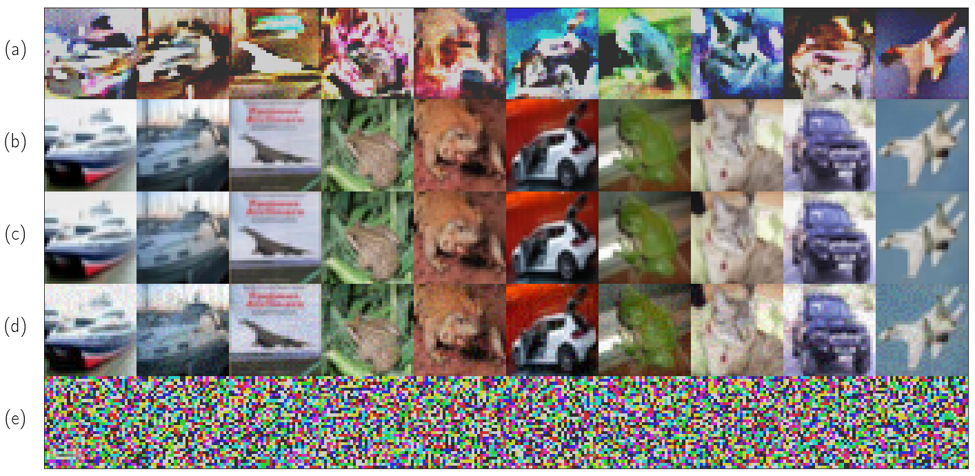
Figure 2: Magnified perturbation and adversarial examples generated by our proposed method vs. bandit attacks (Ilyas et al., 2019). As can be seen, the proposed method generates more realistic adversaries by using a flow-based model as its prior. (a) our method magnified perturbation (b) our method adversarial example (c) clean image (d) bandits adversarial example (e) bandits magnified perturbation.

Table 1: Attack success rate (in %, higher is better) to generate an adversarial example for CIFAR-10 (Krizhevsky & Hinton, 2009) test data. Clean data accuracy and white-box PGD-100 attack success rate are also shown as a reference. All attacks are with respect to the $\ell_{\infty}$ norm with $\epsilon=8/255$.

		Attack
Defense	Clean Acc.(%)	PGD-100	NES	Bandits	Flow-based (ours)
Vanilla	$91.77$	$100$	$99.53$	$98.68$	$99.12$
FreeAdv	$81.29$	$47.52$	$23.45$	$37.10$	$41.06$
FastAdv	$86.33$	$46.37$	$20.15$	$36.70$	$40.06$
RotNetAdv	$86.58$	$46.59$	$20.64$	$36.67$	$40.50$

Table 2: Average and median of the number of queries used to generate an adversarial example for scenarios of Table 1.

	Avg. of Queries $\downarrow$			Med. of Queries $\downarrow$
Defense	NES	Bandits	Flow-based (ours)	NES	Bandits	Flow-based (ours)
Vanilla	$458.50$	$524.14$	$991.98$	$300$	$156$	$460$
FreeAdv	$629.38$	$1430.30$	$842.37$	$100$	$463$	$180$
FastAdv	$1465.51$	$1425.78$	$904.78$	$800$	$454$	$200$
RotNetAdv	$1526.46$	$1470.35$	$821.80$	$800$	$520$	$180$

Next, we select a Wide-ResNet-32 (Zagoruyko & Komodakis, 2016) with width $10$ as our classifier architecture. This classifier is trained in both vanilla and defended fashions. For the defended case, we use free (Shafahi et al., 2019) and fast (Wong et al., 2020) adversarial training alongside adversarial training with auxiliary rotations (Hendrycks et al., 2019). Each one of these classifiers is trained with respect to the $\ell_{\infty}$ norm with $\epsilon=8/255$.

Once the training is done, we can then perform our proposed black-box adversarial attack. To this end, we try to generate an adversary from CIFAR-10 unseen test data. An attack is counted successful if it can change the classifier decision about a correctly classified image in less than $10,000$ queries. We compare our method against NES (Ilyas et al., 2018) and bandits with time and data-dependent priors (Ilyas et al., 2019). The hyperparameters of each method are given in Tables 4-6 in the Appendix.

Tables 1 and 2 show the attack success rate as well as the average and median of the number of queries for attacking nominated DNN classifiers. As can be seen, the proposed method can improve the performance of baselines in attacking defended classifiers in both attack strength (success rate) and efficiency (number of queries). Also, we see that the number of required queries for the proposed method remains almost consistent for both vanilla and defended classifiers. However, this is not generally the case for the other methods, and their performance heavily depends on the classifier type. Furthermore, as shown in Figure 2, the adversarial examples generated by the proposed method look less suspicious in contrast to bandit attacks (Ilyas et al., 2019). Also, we see that the perturbations generated by our approach are disguised in the underlying image structure. However, bandit attack (Ilyas et al., 2019) perturbations do not have this property and look like an additive noise.

5 Conclusion

In this paper, we proposed a novel black-box adversarial attack method using normalizing flows. In particular, we utilize a pre-trained flow-based model to search in the vicinity of the base distribution representation of the target image and generate an adversarial example. Due to the smoothness of image manifolds in normalizing flows, our adversarial examples look natural and unnoticeable. This way, we can generate adversaries that can compete with well-known methods in terms of strength and efficiency. We hope that this work can be inspiring in exploiting such methods for adversarial machine learning and lead to finding statistical treatments to DNNs’ adversarial vulnerabilities.

Appendix

Appendix A Experimental Settings

Table 3: Hyperparameters used in training flow-based part of our approach.

Optimizer	Adam
Scheduler	Exponential
Initial learning rate	$10^{-4}$
Final learning rate	$10^{-6}$
Batch size	$64$
Epochs	$350$
Multi-scale levels	$2$
Each level network type	CNN-FC
High-res transformation blocks	$4$
Low-res transformation blocks	$6$
FC transformation blocks	$6$
$\alpha$ (clamping hyperparameter)	$1.5$
CNN layers hidden channels	$128$
FC layers internal width	$128$
Activation function	Leaky ReLU
Leaky slope	$0.1$

Table 4: Hyperparameters of query-limited NES attack (Ilyas et al., 2018).

Hyperparameter	Vanilla	Defended
$\sigma$ (noise std.)	$0.1$	$0.001$
Sample size	$50$	$100$
Learning rate	$0.01$	$0.01$

Table 5: Hyperparameters of bandits with time and data-dependent priors (Ilyas et al., 2019).

Hyperparameter	Vanilla	Defended
OCO learning rate	$100$	$0.1$
Image learning rate	$0.01$	$0.01$
Bandit exploration	$0.1$	$0.1$
Finite difference probe	$0.1$	$0.1$
Tile size	$(6\mathrm{px})^{2}$	$(4\mathrm{px})^{2}$

Table 6: Hyperparameters of our flow-based adversarial attack.

Hyperparameter	Value
$\sigma$ (noise std.)	$0.1$
Sample size	$20$
$k$ (samples used to update $\boldsymbol{\mu}$)	$4$
Maximum iteration	$500$

References

- Ardizzone et al. (2019) Ardizzone, L., Lüth, C., Kruse, J., Rother, C., and Köthe, U. Guided image generation with conditional invertible neural networks. CoRR, abs/1907.02392, 2019.
- Baluja & Fischer (2018) Baluja, S. and Fischer, I. Learning to attack: Adversarial transformation networks. In Proceedings of the 32nd AAAI Conference on Artificial Intelligence, pp. 2687–2695, 2018.
- Carlini & Wagner (2017) Carlini, N. and Wagner, D. Towards evaluating the robustness of neural networks. In Proceedings of the 2017 IEEE Symposium on Security and Privacy (SP), pp. 39–57, 2017.
- Dinh et al. (2015) Dinh, L., Krueger, D., and Bengio, Y. NICE: non-linear independent components estimation. In Workshop Track Proceedings of the 3rd International Conference on Learning Representations (ICLR), 2015.
- Dinh et al. (2017) Dinh, L., Sohl-Dickstein, J., and Bengio, S. Density estimation using real NVP. In Proceedings of the 5th International Conference on Learning Representations (ICLR), 2017.
- Dolatabadi et al. (2020) Dolatabadi, H. M., Erfani, S. M., and Leckie, C. Invertible generative modeling using linear rational splines. In Proceedings of the 23rd International Conference on Artificial Intelligence and Statistics (AISTATS), pp. 4236–4246, 2020.
- Durkan et al. (2019a) Durkan, C., Bekasov, A., Murray, I., and Papamakarios, G. Cubic-spline flows. In Workshop on Invertible Neural Nets and Normalizing Flows of 36th International Conference on Machine Learning (ICML), 2019a.
- Durkan et al. (2019b) Durkan, C., Bekasov, A., Murray, I., and Papamakarios, G. Neural spline flows. In Proceedings of the Advances in Neural Information Processing Systems 32: Annual Conference on Neural Information Processing Systems (NeurIPS), pp. 7511–7522, 2019b.
- He et al. (2016) He, K., Zhang, X., Ren, S., and Sun, J. Deep residual learning for image recognition. In Proceedings of the 2016 IEEE Conference on Computer Vision and Pattern Recognition (CVPR), pp. 770–778, 2016.
- Hendrycks et al. (2019) Hendrycks, D., Mazeika, M., Kadavath, S., and Song, D. Using self-supervised learning can improve model robustness and uncertainty. In Proceedings of the Advances in Neural Information Processing Systems 32: Annual Conference on Neural Information Processing Systems (NeurIPS), pp. 15637–15648, 2019.
- Ilyas et al. (2018) Ilyas, A., Engstrom, L., Athalye, A., and Lin, J. Black-box adversarial attacks with limited queries and information. In Proceedings of the 35th International Conference on Machine Learning (ICML), pp. 2142–2151, 2018.
- Ilyas et al. (2019) Ilyas, A., Engstrom, L., and Madry, A. Prior convictions: Black-box adversarial attacks with bandits and priors. In Proceedings of the 7th International Conference on Learning Representations (ICLR), 2019.
- Jacobsen et al. (2018) Jacobsen, J., Smeulders, A. W. M., and Oyallon, E. i-RevNet: Deep invertible networks. In Proceedings of the 6th International Conference on Learning Representations (ICLR), 2018.
- Kingma & Ba (2015) Kingma, D. P. and Ba, J. Adam: A method for stochastic optimization. In Proceedings of the 3rd International Conference on Learning Representations (ICLR), 2015.
- Kingma & Dhariwal (2018) Kingma, D. P. and Dhariwal, P. Glow: Generative flow with invertible 1x1 convolutions. In Proceedings of the Advances in Neural Information Processing Systems 31: Annual Conference on Neural Information Processing Systems (NeurIPS), pp. 10236–10245, 2018.
- Kobyzev et al. (2019) Kobyzev, I., Prince, S., and Brubaker, M. A. Normalizing flows: Introduction and ideas. CoRR, abs/1908.09257, 2019.
- Krizhevsky & Hinton (2009) Krizhevsky, A. and Hinton, G. Learning multiple layers of features from tiny images. Master’s thesis, Department of Computer Science, University of Toronto, 2009.
- Müller et al. (2019) Müller, T., McWilliams, B., Rousselle, F., Gross, M., and Novák, J. Neural importance sampling. ACM Transactions on Graphics, 38(5):1–19, 2019.
- Papamakarios et al. (2019) Papamakarios, G., Nalisnick, E., Rezende, D. J., Mohamed, S., and Lakshminarayanan, B. Normalizing flows for probabilistic modeling and inference. CoRR, abs/1912.02762, 2019.
- Rezende & Mohamed (2015) Rezende, D. J. and Mohamed, S. Variational inference with normalizing flows. In Proceedings of the 32nd International Conference on Machine Learning (ICML), pp. 1530–1538, 2015.
- Shafahi et al. (2019) Shafahi, A., Najibi, M., Ghiasi, A., Xu, Z., Dickerson, J. P., Studer, C., Davis, L. S., Taylor, G., and Goldstein, T. Adversarial training for free! In Proceedings of the Advances in Neural Information Processing Systems 32: Annual Conference on Neural Information Processing Systems (NeurIPS), pp. 3353–3364, 2019.
- Song et al. (2018) Song, Y., Shu, R., Kushman, N., and Ermon, S. Constructing unrestricted adversarial examples with generative models. In Proceedings of the Advances in Neural Information Processing Systems 31: Annual Conference on Neural Information Processing Systems (NeurIPS), pp. 8322–8333, 2018.
- Szegedy et al. (2014) Szegedy, C., Zaremba, W., Sutskever, I., Bruna, J., Erhan, D., Goodfellow, I. J., and Fergus, R. Intriguing properties of neural networks. In Proceedings of the 2nd International Conference on Learning Representations (ICLR), 2014.
- Tabak & Turner (2013) Tabak, E. G. and Turner, C. V. A family of nonparametric density estimation algorithms. Communications on Pure and Applied Mathematics, 66(2):145–164, 2013.
- Wang & Yu (2019) Wang, H. and Yu, C. A direct approach to robust deep learning using adversarial networks. In Proceedings of the 7th International Conference on Learning Representations (ICLR), 2019.
- Wong et al. (2020) Wong, E., Rice, L., and Kolter, J. Z. Fast is better than free: Revisiting adversarial training. In Proceedings of the 8th International Conference on Learning Representations (ICLR), 2020.
- Xiao et al. (2018) Xiao, C., Li, B., Zhu, J., He, W., Liu, M., and Song, D. Generating adversarial examples with adversarial networks. In Proceedings of the 27th International Joint Conference on Artificial Intelligence (IJCAI), pp. 3905–3911, 2018.
- Yuan et al. (2019) Yuan, X., He, P., Zhu, Q., and Li, X. Adversarial examples: Attacks and defenses for deep learning. IEEE Transactions on Neural Networks and Learning Systems, 30(9):2805–2824, 2019.
- Zagoruyko & Komodakis (2016) Zagoruyko, S. and Komodakis, N. Wide residual networks. In Proceedings of the British Machine Vision Conference (BMVC), 2016.