Second and third harmonics generation by coherent sub-THz radiation at induced Lifshitz transitions in gapped bilayer graphene

Abstract

Using the microscopic nonlinear quantum theory of interaction of strong coherent electromagnetic radiation with a gapped bilayer graphene is developed for high harmonic generation at low-energy photon excitation- induced Lifshitz transitions. The Liouville-von Neumann equation for the density matrix is solved numerically at the nonadiabatic multiphoton excitation regime. By numerical solutions, we examine the rates of the second and third harmonics generation at the particle-hole annihilation in induced Lifshitz transitions by the two linearly polarized coherent electromagnetic waves propagating in opposite directions. The obtained results show that the gapped bilayer graphene can serve as an effective medium for generation of even and odd high harmonics in the sub-THz domain of frequencies.

I Introduction

Many quantum electrodynamic nonlinear phenomena induced by strong laser radiation in condensed matter, specifically in graphene/nanostructures, have significant contribution in low-energy physics and nano-opto-electronics and have been systematically investigated mainly in case of monolayer graphene 1 ; 1bb ; 2 that has been conditioned by unique physical properties of such two-dimensional (2D) nanosystem of atomic thickness 1 , 1bb . On the other hand, for induced electrodynamic phenomena in 2D atomic systems-nanostructures a bilayer graphene ($AB$-stacked) is of great interest too, since its electronic states are considerably richer than those for monolayer graphene, and multiphoton resonant excitation with high-harmonic generation (HHG) via nonlinear channels in bilayer graphene were also considered hhg1 ; Abook ; hhg2 . The pioneer studies of laser-induced HHG process in recent decades were made generally in gaseous media, while it is of interest the investigation of HHG and related processes in low-dimensional nanostructures, such as graphene and its derivatives H2 ; Mer ; Mer1 ; H3 ; H4 ; H6 ; H7 ; H8 ; H9 ; H99 ; H10 ; H11 ; H12 ; H12a ; H13 ; H14 ; H15 ; H16 ; H17 ; H18 ; H19 ; H21 , bulk crystals s1 ; s2 ; s3 ; s5 ; s6 ; s7 , hexagonal boron nitride BN , monolayer transition metal dichalcogenides TMD ; TMD1 ; TMD11 , topological insulator TI , TII , in monolayers of black phosphorus phosph , buckled 2D hexagonal nanostructures Mer2019 , solids corcumsolid , semimetal , as well as in other 2D systems twodem1 ; twodem2 ; twodem3 . The 2D nanosystems enable to develop important technological applications. The quantum cascade laser is one of such examples QCL using the physical phenomena in 2D systems such as the quantum Hall effect Abook . The nonlinear coherent response in $AB$-stacked bilayer graphene under the influence of intense electromagnetic radiation leads to the modification of quasi-energy spectrum, the induction of valley polarized currents 26b , 27b as well as the second and third-order nonlinear-optical effects 28b ; 29b ; 30b ; 31b . Moreover, the bilayer graphene system represents a unique system in which the topology of the band structure can be externally influenced and chosen. The bilayer graphene is a highly tunable material: not only one can tune the Fermi energy using standard gates, as in single-layer graphene, but the band structure can also be modified by external perturbations such as transverse electric fields or strain 1a ; 1ab ; 1aa ; 9 ; 22b ; 24b ; Liftrans . Particularly, due to the realization of a widely tunable electronic bandgap in an electrically gated bilayer graphene 9 , 10 ; 10a ; 16 , it is of interest to consider HHG process in the strong wave-bilayer graphene coupling regime with a bandgap induced by an external constant electric field as a condensed matter material with nontrivial topology Mer2019 , in particular, with the bands acquiring Berry curvature Berry . Moreover, with the current technology 16 one can make such large gaps in $AB$-stacked bilayer graphene, which is sufficient to produce field-effect transistors with a high on-off ratio not only at cryogenic temperatures but at room-temperature Ber1 , transist .

In addition, it is known the graphene-based low energy photon-counting photodetector of different applications, in areas as diverse as medical and space sciences or security applications. The tunable bandgap in bilayer graphene may enable sensitive photon-counting photodetectors to operate with a trade-off between resolution and operational temperatures, with resulting operational benefits. Note that the large bandgap can also make possible effective room temperature HHG H14 in bilayer graphene, which is suppressed in intrinsic bilayer graphene H3 . Unfortunately, the effective pump wave-induced Lifshitz transitions (with photon energy much smaller than Lifshitz energy) in $AB$-stacked gapped bilayer graphene are less investigated.

In the present paper, with the help of the numerical simulations in a microscopic nonlinear quantum theory of interaction of $AB$-stacked gapped bilayer graphene with the moderately strong laser radiation, we find out the optimal values of the main parameters, in particular, for bandgap, pump wave intensity, graphene temperature for practically significant case in high-order harmonics coherent emission in the particle low-energy region of the induced Lifshitz transitions (the fragmentation of the singly-connected Fermi line into four separate pieces) 22b , Lifshitz ; Lif1 ; Lif2 . The Liouville-von Neumann equation is treated numerically for the generation of the higher (here -second, third) harmonics in the multiphoton excitation regime near the Dirac points of the Brillouin zone. We consider the harmonic generation process in the nonadiabatic regime of interaction when the Keldysh parameter is of the order of unity. The picture of the multiphoton excitation of the Fermi-Dirac sea and the trigonal warping effect is also revealed. We examine the rates of the HHG at the particle-hole annihilation in the strong effective field of two linearly polarized plane electromagnetic waves, propagating in opposite direction for practically optimal parameters of the considering system. Due to the special magnitudes of the bandgap, we can operate with the sample temperature. The obtained results show that for specially chosen values of the corresponding characteristic parameters of this process we can use gapped bilayer graphene as a convenient nonlinear medium to generate the higher harmonics of the pump wave with an effective yield in the sub-THz and THz domains of the spectrum, at the graphene temperatures of higher than the cryogenic temperatures.

The paper is organized as follows. In Sec. II the set of equations for a single-particle density matrix is formulated and numerically solved in the multiphoton interaction regime. In Sec. III, we consider the problem of harmonics generation at the low-energy excitation of gapped bilayer graphene. Finally, conclusions are given in Sec. IV.

II Basic theory

At the higher harmonic emission process in gapped bilayer graphene during the coherent electromagnetic radiation-induced Lifshitz transitions with the energies much smaller than the Lifshitz energy $\mathcal{E}_{L}$ have some peculiarities Lifshitz ; Lif1 ; Lif2 , 46bb ; 47bb ; 48bb ; 49bb . The Lifshitz transition someone is unique with thermoelectric properties of bilayer graphene thermoelectric . Two touching parabolas of the Fermi surface are broken into four separate ‘pockets’. However, as opposed to bulk graphite, the external perturbations like the strain 19bb , 20bb or electric field 21bb can modify the topology of the electronic dispersion and change the energy of the Lifshitz transition which connects regions of different Fermi contour topologies 22bb . Moreover, due to the two-dimensional nature of bilayer graphene, its chemical potential and its topology can be tuned with electrostatic gates 1 , simplifying experimental studies of the Lifshitz transition. By the way, in unperturbed bilayer graphene, it is achieved at low energies $\mathcal{E}_{L}\sim 1$ $\mathrm{meV}$. To induce the asymmetry, a chemical doping can be used 1a or external gates 1ab can be patterned. This induced asymmetry opens a bandgap between the two layers of the bilayer graphene 22b , 46bb ; 47bb ; 48bb ; 49bb . As is shown in 22bb , particularly for an induced asymmetry $U=100$ $\mathrm{meV,}$ the Lifshitz transition occurs at the higher energy $\mathcal{E}_{L}\sim 1.6$ $\mathrm{meV}$. One can conclude from the estimate given in 22bb that the experimental observation of the Lifshitz transition should be facilitated by the layer-asymmetry induced bandgap and that, the wider the gap, the more enhanced the visibility of this effect.

At an intraband transitions the interaction of a particle with the wave at the THz or sub-THz photon low-energies $\hbar\omega\ll\mathcal{E}_{L}$, characterizes by the effective interaction parameter $\chi$ H3 :

$$\chi=eE_{0}\mathrm{v}_{3}/(\hbar\omega^{2}),$$ (1)

where $E_{0}$ is the wave strength, $\omega$ is the wave frequency, $e$ is the electron charge. Due to the gap, the interband transitions are characterized by so-called Keldysh Keld1 ; Keld2 parameter expressed in the form:

$$\gamma=\omega\sqrt{m_{\ast}U}/\left(eE_{0}\right)=\chi^{-1}\mathrm{v}_{3}\sqrt{m_{\ast}U}/\left(\hbar\omega\right).$$ (2)

Here $U$ is the bandgap energy, $\hbar$ is the Planck constant; $m_{\ast}=\gamma_{1}/(2\mathrm{v}_{F}^{2})$ is the effective mass ($\mathrm{v}_{F}$ is the Fermi velocity in monolayer graphene); $\mathrm{v}_{3}=\sqrt{3}a\gamma_{3}/(2\hbar)\approx\mathrm{v}_{F}/8$ is the effective velocity related to oblique interlayer hopping $\gamma_{3}=0.32$ $\mathrm{eV}$ ($a\approx 0.246$ $\mathrm{nm}$ is the distance between the nearest $A$ sites), $\gamma_{1}\simeq 0.39$ $\mathrm{eV.}$

For the gapped materials, the Keldysh parameter gives the character of the ionization process which with the electron-hole pair creation is the first step of HHG. In the limit of $\gamma\gg 1$, the multiphoton ionization dominates in the ionization process. In the so-called nonadiabatic regime $\gamma\sim 1$, both multiphoton ionization and tunneling ionization can take place. In the limit of $\gamma\ll 1$, the tunneling ionization dominates. For the considered case, the ionization process reduces to the transfer of the electron from the valence band into the conduction band that is the creation of an electron-hole pair. Since the interband transitions can be neglected when $\gamma\gg 1$, then the wavefield cannot provide enough energy for the creation of an electron-hole pair, and the generation of harmonics is suppressed. So that, in the nonadiabatic regime due to the large ionization probabilities the intensity of harmonics can be significantly enhanced compared with tunneling one H14 , H19 . If $\gamma\sim 1$ or $\gamma\ll 1$, interband transitions take place. From this point of view, condensed matter materials with bilayer graphene are preferable due to the tunable bandgap with nontrivial topology.

In the present paper, we will consider the nonadiabatic regime for the generation of HHG at $\chi\sim 1$ and $\gamma\sim 1$, when the multiphoton effects become essential. Our consideration is mainly focused on the low photon energies. Note that the average intensity of the wave expressed by $\chi$ can be given as

$$I_{\chi}=\chi^{2}\times 6\times 10^{10}\mathrm{Wcm}^{-2}(\hbar\omega/\mathrm{eV})^{3},$$

so the required intensity $I_{\chi}$ for the nonlinear regime  strongly depends on the photon energy. Particularly, for the photons with the energies $0.4-0.9$ $\mathrm{meV,}$ the multiphoton interaction regime can be achieved at the intensities $I_{\chi}=1-10^{2}\mathrm{\ Wcm}^{-2}$. Note, that modern photonic-based THz and sub-THz (with energies $0.4-1.24$ $\mathrm{meV}$) sources include quantum cascade lasers and can achieve admirable output powers, mainly at cryogenic temperatures, whereas used in conjunction with nonlinear crystals can make microwatts of tunable continuous wave THz at room temperature subTHz . Unfortunately, all of these sources offer impressive performance in their own ways, but none so far are easily integrated into larger digital electronic systems, which is arguably their biggest downfall for communication systems subTHz1 .

In the following we use the microscopic nonlinear quantum theory of interaction of coherent electromagnetic radiation with gapped bilayer graphene which was developed in H14 , H19 . To get the sub-THz frequencies, let propose two linearly polarized plane electromagnetic waves with carrier frequency $\omega$ and slowly varying amplitude of the electric field $E_{a}f(t)$:

$$E_{1}\left(t\right)=\widehat{\mathbf{e}}E_{a}f(t)\cos\left(\omega t+\mathbf{kr}\right),$$ (3)

$$E_{2}\left(t\right)=\widehat{\mathbf{e}}E_{a}f(t)\cos\left(\omega t-\mathbf{kr}\right),$$ (4)

propagating in opposite directions in a vacuum. We assume that the pump wave wavelength $\lambda\gg a$, where $a$ is the characteristic size of the carbon system–the distance between the nearest $A$ sites (for the HHG this condition is always satisfied). In considering case of a standing wave formed by the laser beams (4), a significant input in the HHG process is conditioned by the Dirac points situated near the stationary maxima of the standing wave. For these points, the magnetic fields of the counterpropagating waves cancel each other Abook , physrevA2011 , plasma2011 . Since the HHG is essentially produced at the lengths $l\ll\lambda$ near the electric field maximums, we assume the effective field in the plane of the graphene sheets ($XY$) to be:

$$\mathbf{E}\left(t\right)=f\left(t\right)E_{0}\widehat{\mathbf{e}}\cos\omega t,$$ (5)

where $E_{0}=2E_{a}$, and $\widehat{\mathbf{e}}$ is the unit polarization vector. The pump wave slowly varying envelope is described by the function:

$$f\left(t\right)=\left\{\begin{array}[]{cc}\sin^{2}\left(\pi t/\mathcal{T}\right),&0\leq t\leq\mathcal{T},\\ 0,&t<0,t>\mathcal{T},\end{array}\right.,$$ (6)

where $\mathcal{T}$ characterizes the pulse duration and is taken to be $\mathcal{T}=10\mathcal{T}_{0}$, $\phi$ is the pump wave polarization parameter, $\mathcal{T}_{0}=2\pi/\omega$.

In $AB$-stacked gapped bilayer graphene, the low-energy excitations $\left|\mathcal{E}_{\sigma}\right|<\gamma_{1}\simeq 0.39$ $\mathrm{eV}$ in the vicinity of the Dirac points $K_{\zeta}$ can be described by an effective single-particle Hamiltonian 9 ; 22b ; 24b :

$$\widehat{H}_{\zeta}=\left(\begin{array}[]{cc}\frac{U}{2}&g_{\zeta}^{\ast}\left(\mathbf{p}\right)\\ g_{\zeta}\left(\mathbf{p}\right)&-\frac{U}{2}\end{array}\right),$$ (7)

where

$$g_{\zeta}\left(\mathbf{p}\right)=-\frac{1}{2m_{\ast}}\left(\zeta\widehat{p}_{x}+i\widehat{p}_{y}\right)^{2}+\mathrm{v}_{3}\left(\zeta\widehat{p}_{x}-i\widehat{p}_{y}\right),$$ (8)

$\mathbf{\hat{p}}=\left\{\widehat{p}_{x},\widehat{p}_{y}\right\}$ is the electron momentum operator, $\zeta=\pm 1$ is the valley quantum number. The diagonal elements in Eq. (7) correspond to opened gap $U$. The first term in Eq. (8) gives a pair of parabolic bands $\mathcal{E}=\pm p^{2}/(2m_{\ast})$, and the second term connecting with $\gamma_{3}$ causes trigonal warping in the band dispersion. The spin and the valley quantum numbers are conserved. There is no degeneracy upon the valley quantum number $\zeta$ for the issue considered. However, since there are no intervalley transitions, the valley index $\zeta$ can be considered as a parameter.

The eigenstates of the effective Hamiltonian (7) are the spinors,

$$\Psi_{\sigma}(\mathbf{r})=\frac{1}{\sqrt{S}}|\sigma,\mathbf{p}\rangle e^{\frac{i}{\hbar}\mathbf{pr}}$$ (9)

where

$$|\sigma,\mathbf{p}\rangle=\frac{1}{\sqrt{S}}\sqrt{\frac{\mathcal{E}_{\sigma}+\frac{U}{2}}{2\mathcal{E}_{\sigma}}}\left(\begin{array}[]{c}1\\ \frac{1}{\mathcal{E}_{\sigma}+\frac{U}{2}}\Upsilon\left(\mathbf{p}\right)\end{array}\right),$$ (10)

$$\Upsilon\left(\mathbf{p}\right)=-\frac{p^{2}}{2m}e^{i2\zeta\vartheta}+\zeta\mathrm{v}_{3}pe^{-i\zeta\vartheta}.$$ (11)

$\vartheta=\arctan\left(p_{y}/p_{x}\right)$, $\sigma$ is the band index: $\sigma=1$ and $\sigma=-1$ for conduction and valence bands, respectively; and $S$ is the quantization area. The corresponding eigenenergies are

$$\mathcal{E}_{\sigma}\left(\mathbf{p}\right)=\sigma\sqrt{\frac{U^{2}}{4}+\left(\mathrm{v}_{3}p\right)^{2}-\zeta\frac{\mathrm{v}_{3}p^{3}}{m}\cos 3\vartheta+\left(\frac{p^{2}}{2m}\right)^{2}}.$$ (12)

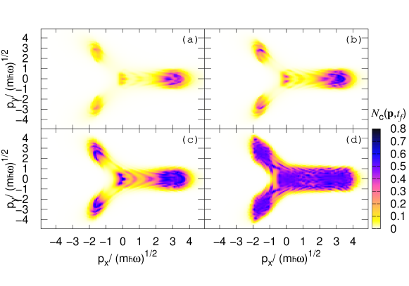
Figure 1: (Color online) Particle distribution function $N_{c}(\mathbf{p},t_{f})$ (in arbitrary units) after the interaction at the instant $t_{f}=10T$, as a function of scaled dimensionless momentum components is shown. The effective field is assumed to be linearly polarized along the $y$ axis. Multiphoton excitation with the trigonal warping effect for low-energy photon excitation-induced Lifshitz transitions at the photon energy $\hbar\omega=\mathcal{E}_{L}/1.1$ $\simeq$ $0.9$ $\mathrm{meV}$, the temperature $T/\hbar\omega=0.4$ are demonstrated at dimensionless intensity parameter $\chi=1$ for valley $\zeta=-1$. (a)–(d) correspond to the gap energy $U=5$ $\mathrm{meV},$ $4$ $\mathrm{meV,}$ $3$ $\mathrm{meV}$ and $0.0008$ $\mathrm{meV,}$ respectively.

Due to the second quantized technique, we can write the Fermi-Dirac field operator in the form of an expansion in the free states, given in (9), that is,

$$\widehat{\Psi}(\mathbf{r},t)=\sum\limits_{\mathbf{p,}\sigma}\widehat{a}_{\mathbf{p},\sigma}(t)\Psi_{\sigma}(\mathbf{r}),$$ (13)

where $\widehat{a}_{\mathbf{p},\sigma}(t)$ ($\widehat{a}_{\mathbf{p},\sigma}^{+}(t)$) is the annihilation (creation) operator for an electron with momentum $\mathbf{p}$ which satisfy the usual fermionic anticommutation rules at equal times. The single-particle Hamiltonian in the presence of a uniform time-dependent electric field $E(t)$ can be expressed in the form:

$$\widehat{H}_{s}=\widehat{H}_{\zeta}+\left(\begin{array}[]{cc}e\mathbf{rE}\left(t\right)&0\\ 0&e\mathbf{rE}\left(t\right)\end{array}\right),$$ (14)

where for the interaction Hamiltonian we have used a length gauge, describing the interaction by the potential energy Corkum , 32b . Taking into account expansion (13), the second quantized total Hamiltonian can be expressed in the form:

$$\widehat{H}=\sum\limits_{\sigma,\mathbf{p}}\mathcal{E}_{\sigma}\left(\mathbf{p}\right)\widehat{a}_{\sigma\mathbf{p}}^{+}\widehat{a}_{\sigma\mathbf{p}}+\widehat{H}_{\mathrm{s}},$$ (15)

where the light–matter interaction part is given in terms of the gauge-independent field $\mathbf{E}\left(t\right)$ as follow:

$$\widehat{H}_{\mathrm{s}}=ie\sum\limits_{\mathbf{p,p}^{\prime},\sigma}\delta_{\mathbf{p}^{\prime}\mathbf{p}}\partial_{\mathbf{p}^{\prime}}\mathbf{E}\left(t\right)\widehat{a}_{\mathbf{p},\sigma}^{\dagger}\widehat{a}_{\mathbf{p}^{\prime},\sigma^{\prime}}\$$

$$+\sum\limits_{\mathbf{p},\sigma}\mathbf{E}\left(t\right)\left(\mathbf{D}_{\mathrm{t}}\left(\sigma,\mathbf{p}\right)\widehat{a}_{\mathbf{p},\sigma}^{+}\widehat{a}_{\mathbf{p},-\sigma}+\mathbf{D}_{\mathrm{m}}\left(\sigma,\mathbf{p}\right)\widehat{a}_{\mathbf{p},\sigma}^{+}\widehat{a}_{\mathbf{p},\sigma}\right),$$ (16)

where

$$\mathbf{D}_{\mathrm{t}}\left(\sigma,\mathbf{p}\right)=\hbar e\langle\sigma,\mathbf{p}|i\partial_{\mathbf{p}}|-\sigma,\mathbf{p}\rangle$$ (17)

is the transition dipole moment and

$$\mathbf{D}_{\mathrm{m}}\left(\sigma,\mathbf{p}\right)=\hbar e\langle\sigma,\mathbf{p}|i\partial_{\mathbf{p}}|\sigma,\mathbf{p}\rangle$$ (18)

is the Berry connection or mean dipole moment, which are given in Appendix.

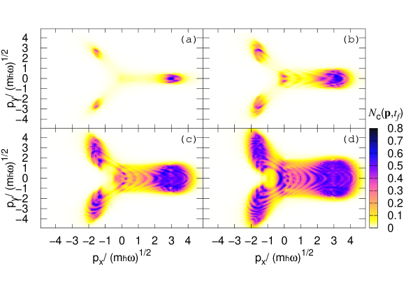
Figure 2: (Color online) Creation of a particle-hole pair in bilayer graphene at multiphoton resonant excitation. Particle distribution function $N_{c}(\mathbf{p},t_{f})$ (in arbitrary units) after the interaction is displayed at various intensities corresponding to : (a) $\chi=0.5$, (b) $\chi=1$, (c) $\chi=1.5$, and (d) $\chi=2$. The temperature is taken to be $T/\hbar\omega=0.4$. The effective field is assumed to be linearly polarized along the $y$ axis with the photon energy $\hbar\omega=\mathcal{E}_{L}/1.1$ $\simeq$ $0.9$ $\mathrm{meV}$ and gap energy is $U=4$ $\mathrm{meV}$. The results are for the valley $\zeta=-1$.

Multiphoton interaction of a bilayer graphene with a strong radiation field will be described by the Liouville–von Neumann equation for a single-particle density matrix (see Appendix equations (29), (30)). As an initial state, we assume an ideal Fermi gas in equilibrium with chemical potential to be zero. We will solve the set of Eqs. (31), and followed from the last closed set of differential equations (32), (33) given in the Appendix, for the functions $N_{\mathrm{v}}(\mathbf{p},t)$, $N_{c}(\mathbf{p},t)$, $P(\mathbf{p},t)$, taking into account the initial conditions:

$$P(\mathbf{p},0)=0;\ N_{c}(\mathbf{p},0)=\frac{1}{1+e^{\mathcal{E}_{1}\left(\mathbf{p}\right)/T}};$$ (19)

$$N_{\mathrm{v}}(\mathbf{p},0)=1-N_{c}(\mathbf{p},0).$$ (20)

Here $T$ is the temperature in energy units. Note that we will incorporate relaxation processes into Liouville–von Neumann equation with inhomogeneous phenomenological damping rate $\Gamma$, since homogeneous relaxation processes are slow compared with inhomogeneous.

The set of equations (32), (33), and (34) can not be solved analytically. For the numerical solution we made a change of variables and transform the equations with partial derivatives into ordinary ones. The new variables are $t$ and $\widetilde{\mathbf{p}}=\mathbf{p}-\mathbf{p}_{E}$ $\left(t\right)$, where

$$\mathbf{p}_{E}\left(t\right)=-e\int_{0}^{t}\mathbf{E}\left(t^{\prime}\right)dt^{\prime}$$ (21)

is the classical momentum given by the wave field. After these transformations, the integration of equations (32), (33), and (34) is performed on a homogeneous grid of $10^{4}$ ($\widetilde{p}_{x},\widetilde{p}_{y}$)-points. For the maximal momentum we take $\widetilde{p}_{\max}/\sqrt{m\hbar\omega}=5$. The time integration is performed with the standard fourth-order Runge-Kutta algorithm. For the relaxation rate we take $\Gamma=0.5\mathcal{T}^{-1}$.

Photoexcitations of the Fermi-Dirac sea - induced Lifshitz transitions, are presented in Figs. 1, 2. The effective wave is assumed to be linearly polarized along the $y$ axis. Similar calculations for a wave linearly polarized along the $x$ axis show qualitatively the same picture. In Fig.1 density plot of the particle distribution function $N_{c}(\mathbf{p},t_{f})$ is shown as a function of scaled dimensionless momentum components after the interaction at the different energy gaps. The pump wave pulse duration is $\mathcal{T}=10\mathcal{T}_{0}\approx 46$ $\mathrm{ps}$. It is clearly seen as the trigonal warping effect describing the deviation of the excited iso-energy contours from circles, which is smeared with the increase of the gap magnitude. In all considering cases, the two touching parabolas are transformed into the four separate “pockets”. Note that trigonal warping is crucial for even-order nonlinearity. As is seen with the increasing of $U$ we approach to perturbative regime $\gamma>1$ and only weak excitation of Fermi-Dirac sea.

Figure 3: The harmonic emission rate (in arbitrary units) of  (a) second $G_{2}$ and (b) third $G_{3}$ order in bilayer graphene at Lifshitz transition versus the intensity parameter $\chi$ is shown for various gap energies. The temperature is taken to be $T/\hbar\omega=0.4$. The effective wave is assumed to be linearly polarized with the frequency $\omega=$ $0.9$ $\mathrm{meV/\hbar}$.

Figure 4: (a) Second $G_{2}$ and (b) third $G_{3}$ harmonic emission rates (in arbitrary units) versus the band gap $U$ for various intensities at the same other parameters as in Fig. 3.

In Fig. 2, we show the photoexcitation depending on the pump wave intensity at fixed sub-THz frequency. For the large values of $\chi$ when $\gamma=1.1$ we clearly see multiphoton excitations. With the increasing wave intensity, the states with the absorption of more photons appear in the Fermi-Dirac sea. At the parameters $\chi\succsim 1$ when $\gamma\simeq 1$, the multiphoton excitation of the Fermi-Dirac sea takes place along the trigonally warped isolines of the quasienergy spectrum modified by the wave field. Thus, the multiphoton probabilities of particle-hole pair production will have maximal values for the iso-energy contours defined by the resonant condition $\mathcal{T}_{0}^{-1}\int\limits_{0}^{\mathcal{T}_{0}}2\mathcal{E}_{1}\left(\widetilde{\mathbf{p}}+\mathbf{p}_{E}\left(t\right),t\right)dt=n\hbar\omega,\ \ n=1,2,3$…These contours are also seen in Fig. 1. The investigations of the temperature dependence of the excitation of the Fermi-Dirac sea are cleared that for considering cases it exhibits a tenuous dependence on the optimal temperatures: the excited isolines are slightly smeared out with temperature increase. This effect is small since $U\gg$ $T$ and one can expect that harmonic spectra will be robust against temperature change in contrast to the gap $U=0$ case where harmonics radiation is suppressed with the increase of temperature in H14 , H19 . So, the temperature dependence was missed.

In the following section, we will investigate the nonlinear response of the bilayer graphene in the process of the second and third-order harmonics generation under the influence of the laser field in the nonadiabatic regime $\gamma\simeq 1$ with the frequencies in sub-THz domain: $\omega=0.4\div 0.9$ $\mathrm{meV/}\hbar$.

III Harmonics generation at induced low-energy transitions in gapped bilayer graphene

In this section, we examine the nonlinear response of a bilayer graphene to harmonic generation process considering the nonadiabatic regime of induced Lifshitz transitions, when the Keldysh parameter is of the order of unity. For the coherent part of the radiation spectrum one needs the mean value of the current density operator,

$$j_{\zeta}=-2e\left\langle\widehat{\Psi}(\mathbf{r},t)\left|\widehat{\mathbf{v}}_{\zeta}\right|\widehat{\Psi}(\mathbf{r},t)\right\rangle.$$ (22)

The velocity operator $\widehat{\mathbf{v}}_{\zeta}=\partial\widehat{H}/\partial\widehat{\mathbf{p}}$ is given in Appendix. Using the Eqs. (22)–(40) and (29), the expectation value of the current for the valley $\zeta$ can be written in the form:

$$\mathbf{j}_{\zeta}\left(t\right)=-\frac{2e}{(2\pi\hbar)^{2}}\int d\mathbf{p}\left\{\mathbf{V}_{1}\left(\mathbf{p}\right)\left(N_{c}(\mathbf{p},t)-N_{\mathrm{v}}(\mathbf{p},t)\right)\right.$$

$$\left.+2\hbar^{-1}i\mathcal{E}_{1}\left(\mathbf{p}\right)\left[\mathbf{D}_{\mathrm{t}}\left(\mathbf{p}\right)P^{\ast}(\mathbf{p},t)-\mathbf{D}_{\mathrm{t}}^{\ast}\left(\mathbf{p}\right)P(\mathbf{p},t)\right]\right\},$$ (23)

where $\mathbf{V}_{1}\left(\mathbf{p}\right)$ is the intraband velocity. In Eq. (23) the first term is the intraband current which conditioned by intraband high harmonics and is generated as a result of the independent motion of carriers in their respective bands. The second term in Eq. (23) describes high harmonics which are generated as a result of the recombination of accelerated electron-hole pairs. Since we study the nonadiabatic regime, the contribution of both mechanisms is essential.

There is no degeneracy upon valley quantum number $\zeta$, so the total current can be obtained by a summation over $\zeta$:

$$j_{x}=j_{1,x}+j_{-1,x};$$ (24)

$$j_{y}=j_{1,y}+j_{-1,y}.$$ (25)

The current density components $j_{x,y}$ are defined as

$$\frac{j_{x,y}}{j_{0}}=G_{x,y}\left(\omega t,\chi,\gamma,\frac{\mathcal{E}_{L}}{\hbar\omega},\frac{T}{\hbar\omega},\frac{U}{\hbar\omega}\right).$$ (26)

Here

$$j_{0}=\frac{e\omega}{\pi^{2}}\sqrt{\frac{m\omega}{\hbar}},$$ (27)

and $G_{x}$ and $G_{y}$ are the dimensionless periodic (for monochromatic wave) functions which parametrically depend on the interaction parameters $\chi$, $\gamma$, scaled Lifshitz energy, and temperature. Thus, using solutions of  Eqs. (32)-(34), and making an integration in Eq. (23), one can calculate the harmonic radiation spectra with the help of a Fourier transform of the function $G_{x,y}(t)$. The emission rate of the $n$th harmonic is proportional to $n^{2}|j_{n}|^{2}$, where $|j_{n}|^{2}$ = $|j_{xn}|^{2}+|j_{yn}|^{2}$, with $j_{xn}$ and $j_{yn}$ being the $n$th Fourier components of the field-induced total current. To find $j_{n}$, the fast Fourier transform algorithm has been used. We use the normalized current density (26) for the plots.

For clarification of harmonics generation due to the multiphoton resonant excitation and particle-hole annihilation, from the coherent superposition states at $\gamma\simeq 1$ initially, we examine the emission rate of the second and third harmonics. The emission rate versus the pump wave strength defined by the parameter $\chi$ at the same wave frequency is demonstrated in Fig. 3 for various gap energies. In Fig. 3, plots for $U=4$ $\mathrm{meV}$ and $U=5$ $\mathrm{meV}$ coincided. As is seen from this figure, for the field intensities $\chi\succsim 1$ at the considering values of the gap energy $U$ we have a strong deviation from power law for the emission rate of the second or third harmonic (in accordance with the perturbation theory $\sim\chi^{2}$ and $\chi^{3}$, respectively). In Fig. 4, the second and third harmonics emission rate, expectantly, is assumed as a function of the energy gap at various intensities defined by the parameter $\chi$ at the same wave frequency. As shown in Fig. 4, all plots have the minimum values at $U=4$ $\mathrm{meV}$. As a result, we find the optimal parameters when the harmonic emission rate is significant at the larger intensity for the considered wave frequency. So, in accordance with the results of Figs. 3 and 4, the intense radiation of the second and third harmonics at the pump-wave-induced particle or hole acceleration and annihilation in gapped graphene can be obtained with the pump wave frequency in the sub-THz domain. Then, as in case of the similar calculations for the intense pump wave or large gap energy $U$ ($U\gg T$) has shown that the emission rate exhibits a tenuous dependence on the temperature.

Figure 5 demonstrates the emission rate dependence on the pump frequency for gapped bilayer graphene. We plot the second and third harmonic emission rates for a gapped bilayer graphene versus the pump frequency for the gap $4$ $\mathrm{meV}$ and various intensity parameters. As was expected and shown from this figure, the emission rate has different maxima at various photon energies and intensities. For third harmonic generation, the maximal value is reached at frequency $\omega=$ $0.9$ $\mathrm{meV/\hbar}$. Concerning the generation of high harmonics up to the far-infrared range, note that this has been demonstrated in the paper H19 where quantum cascade lasers are readily available and can provide higher powers.

Finally, we investigate the physical conditions for considered case of HHG in a bilayer graphene. Let us study the coherent interaction of bilayer graphene with a pump wave in the ultrafast excitation regime, which is correct only for the times $t<\tau_{\min}$, where $\tau_{\min}$ is the minimum of all relaxation times. For the excitations of energies $\mathcal{E}\ll\gamma_{1}=0.39$ $\mathrm{eV}$, the dominant mechanism for relaxation will be electron-phonon coupling via longitudinal acoustic phonons Hwang , Viljas . For the low-temperature limit $T\ll 2\left(c_{ph}/\mathrm{v}_{F}\right)\sqrt{\mathcal{E}\gamma_{1}}$, where $c_{ph}\simeq 2\times 10^{6}$ $\mathrm{cm/s}$ is the velocity of the longitudinal acoustic phonon, the relaxation time for the energy level $\mathcal{E}$ can be estimated as Viljas :

Figure 5: (a) Second $G_{2}$ and (b) third $G_{3}$ harmonic emission rate (in arbitrary units) for bilayer graphene versus $\hbar\omega$ for various intensities. The temperature is taken to be $T/\hbar\omega=0.4$, and the band gap $U=4$ $\mathrm{meV}$. The effective field is assumed to be linearly polarized along the $y$ axis.

$$\tau\left(\mathcal{E}\right)\simeq\left(\frac{\pi D^{2}T^{2}}{8\rho_{m}\hbar^{3}c_{ph}^{3}\mathrm{v}_{F}}\sqrt{\frac{\gamma_{1}}{\mathcal{E}}}\right)^{-1}.$$ (28)

Here $D\simeq 20$ $\mathrm{eV}$ is the electron-phonon coupling constant and $\rho_{m}\simeq 15\times 10^{-8}$ $\mathrm{g/cm}^{2}$ is the mass density of the bilayer graphene. For $\mathcal{E}\simeq 0.9$ $\mathrm{meV}$ at the temperatures $T=0.4\hbar\omega$, from Eq. (28) we obtain $\tau\simeq 50$ $\mathrm{ps}$. Thus, in this energy range one can coherently manipulate with multiphoton transitions in bilayer graphene on the time scales $t\precsim 50\mathrm{ps}$, not taking into account the particle-particle collisions.

Note that the transition currents with comparing the intrinsic graphene $j_{0}$ Mer , Mer1 , for a bilayer graphene is larger by a factor $\left(\gamma_{1}/2\hbar\omega\right)^{1/2}$. Besides, the cutoff harmonic is larger than in case of a monolayer graphene Mer , which is a result of strong nonlinearity caused by trigonal warping. Hence, for considered setups $\hbar\omega\ll\gamma_{1}$ the harmonics’ radiation intensity is at least one order of magnitude larger than in the monolayer graphene.

IV Conclusion

We have presented the microscopic theory of nonlinear interaction of the gapped bilayer graphene with a strong coherent radiation field at low-energy photon Lifshitz transitions. The closed set of differential equations for the single-particle density matrix is solved numerically for a bilayer graphene in the Dirac cone approximation. For the pump wave, the sub-THz frequency range has been taken. Such waves can be produced by the two linearly polarized plane electromagnetic waves of the same frequencies, propagating in opposite. We have considered nonadiabatic wave-induced Lifshitz transitions of Fermi-Dirac sea towards the HHG. It has been shown that the role of the gap in the nonlinear optical response of bilayer graphene is quite considerable. In particular, even-order nonlinear processes are present in contrast to intrinsic bilayer graphene, the cutoff of harmonics increases, and harmonic emission processes become robust against the temperature increase. The obtained results show that the gapped bilayer graphene can serve as an effective medium for the generation of even and odd high harmonics in the THz and sub-THz domain of frequencies, which is sufficient for a new high-speed wireless communication systems development subTHz , subTHz1 . The obtained results certify that the process of high-harmonic generation for sub-THz photons (wavelengths from $0.3$ $\mathrm{mm}\$to $1$ $\mathrm{mm}$) can already be observed for intensities $I_{\chi}=1-10^{3}\mathrm{\ Wcm}^{-2}$ at the temperature of the sample $T<\hbar\omega$. So, bilayer graphene is a very tunable material. The features, such as the Lifshitz transition, can be largely influenced by external parameters such as strain, magnetic fields, or even displacement static electric fields, like to considering case. Bilayer graphene represents therefore a unique system in which the topology of the band structure can be externally influenced and chosen.

V Appendix

Here we present the Liouville–von Neumann equation for a single-particle density matrix

$$\rho_{\alpha,\beta}(\mathbf{p},t)=\langle\widehat{a}_{\mathbf{p},\beta}^{+}\left(t\right)\widehat{a}_{\mathbf{p},\alpha}\left(t\right)\rangle,$$ (29)

where $\widehat{a}_{\mathbf{p},\alpha}\left(t\right)$ obeys the Heisenberg equation

$$i\hbar\frac{\partial\widehat{a}_{\mathbf{p},\alpha}\left(t\right)}{\partial t}=\left[\widehat{a}_{\mathbf{p},\alpha}\left(t\right),\widehat{H}\right].$$ (30)

Note that due to the homogeneity of the problem we only need the $\mathbf{p}$-diagonal elements of the density matrix. Thus, taking into account Eqs. (15)-(30), the evolutionary equation will be

$$i\hbar\frac{\partial\rho_{\alpha,\beta}(\mathbf{p},t)}{\partial t}-i\hbar e\mathbf{E}\left(t\right)\frac{\partial\rho_{\alpha,\beta}(\mathbf{p},t)}{\partial\mathbf{p}}=$$

$$\left(\mathcal{E}_{\alpha}\left(\mathbf{p}\right)-\mathcal{E}_{\beta}\left(\mathbf{p}\right)-i\hbar\Gamma\left(1-\delta_{\alpha\beta}\right)\right)\rho_{\alpha,\beta}(\mathbf{p},t)$$

$$+\mathbf{E}\left(t\right)\left(\mathbf{D}_{\mathrm{m}}\left(\alpha,\mathbf{p}\right)-\mathbf{D}_{\mathrm{m}}\left(\beta,\mathbf{p}\right)\right)\rho_{\alpha,\beta}(\mathbf{p},t)$$

$$+\mathbf{E}\left(t\right)\left[\mathbf{D}_{\mathrm{t}}\left(\alpha,\mathbf{p}\right)\rho_{-\alpha,\beta}(\mathbf{p},t)-\mathbf{D}_{\mathrm{t}}\left(-\beta,\mathbf{p}\right)\rho_{\alpha,-\beta}(\mathbf{p},t)\right],$$ (31)

where $\Gamma$ is the damping rate. In Eq. (31) the diagonal elements represent particle distribution functions for conduction $N_{c}(\mathbf{p},t)=\rho_{1,1}(\mathbf{p},t)$ and valence $N_{\mathrm{v}}(\mathbf{p},t)=\rho_{-1,-1}(\mathbf{p},t)$ bands, and the nondiagonal elements are interband polarization $\rho_{1,-1}(\mathbf{p},t)=P(\mathbf{p},t)$ and its complex conjugate $\rho_{-1,1}(\mathbf{p},t)=P^{\ast}(\mathbf{p},t)$. Thus, we need to solve the closed set of differential equations for these quantities:

$$i\hbar\frac{\partial N_{c}(\mathbf{p},t)}{\partial t}-i\hbar e\mathbf{E}\left(t\right)\frac{\partial N_{c}(\mathbf{p},t)}{\partial\mathbf{p}}=$$

$$\mathbf{E}\left(t\right)\mathbf{D}_{\mathrm{t}}\left(\mathbf{p}\right)P^{\ast}(\mathbf{p},t)-\mathbf{E}\left(t\right)\mathbf{D}_{\mathrm{t}}^{\ast}\left(\mathbf{p}\right)P(\mathbf{p},t),$$ (32)

$$i\hbar\frac{\partial N_{\mathrm{v}}(\mathbf{p},t)}{\partial t}-i\hbar e\mathbf{E}\left(t\right)\frac{\partial N_{\mathrm{v}}(\mathbf{p},t)}{\partial\mathbf{p}}=$$

$$-\mathbf{E}\left(t\right)\mathbf{D}_{\mathrm{t}}\left(\mathbf{p}\right)P^{\ast}(\mathbf{p},t)+\mathbf{E}\left(t\right)\mathbf{D}_{\mathrm{t}}^{\ast}\left(\mathbf{p}\right)P(\mathbf{p},t),$$ (33)

$$i\hbar\frac{\partial P(\mathbf{p},t)}{\partial t}-i\hbar e\mathbf{E}\left(t\right)\frac{\partial P(\mathbf{p},t)}{\partial\mathbf{p}}=$$

$$\left[2\mathcal{E}_{1}\left(\mathbf{p}\right)+\mathbf{E}\left(t\right)\mathbf{D}_{\mathrm{m}}\left(\mathbf{p}\right)-i\hbar\Gamma\right]P(\mathbf{p},t)$$

$$+\mathbf{E}\left(t\right)\mathbf{D}_{\mathrm{t}}\left(\mathbf{p}\right)\left[N_{\mathrm{v}}(\mathbf{p},t)-N_{c}(\mathbf{p},t)\right],$$ (34)

The components of the transition dipole moments are calculated via Eq. (17) by spinor wave functions (10):

$$D_{\mathrm{t}x}\left(\mathbf{p}\right)=-\frac{e\hbar}{2\mathcal{E}_{1}\left(\mathbf{p}\right)\sqrt{\mathcal{E}_{1}^{2}\left(\mathbf{p}\right)-\frac{U^{2}}{4}}}$$

$$\mathbf{\times}\left(\left[\left(\frac{p^{2}}{2m}-m\mathrm{v}_{3}^{2}\right)\frac{\zeta p_{y}}{m}+\frac{\mathrm{v}_{3}}{m}p_{x}p_{y}\right]\right.$$

$$\left.-i\frac{U}{2\mathcal{E}_{1}}\left\{\left(\frac{p^{2}}{2m}+m\mathrm{v}_{3}^{2}\right)\frac{p_{x}}{m}-\frac{3\zeta\mathrm{v}_{3}}{2m}\left(p_{x}^{2}-p_{y}^{2}\right)\right\}\right),$$ (35)

$$D_{\mathrm{t}y}\left(\mathbf{p}\right)=-\frac{e\hbar}{2\mathcal{E}_{1}\left(\mathbf{p}\right)\sqrt{\mathcal{E}_{1}^{2}\left(\mathbf{p}\right)-\frac{U^{2}}{4}}}$$

$$\times\left(\left[\left(-\frac{p^{2}}{2m}+m\mathrm{v}_{3}^{2}\right)\frac{\zeta p_{x}}{m}+\frac{\mathrm{v}_{3}}{2m}\left(p_{x}^{2}-p_{y}^{2}\right)\right]\right.$$

$$\left.-i\frac{U}{2\mathcal{E}_{1}}\left\{\left(\frac{p^{2}}{2m}+m\mathrm{v}_{3}^{2}\right)\frac{p_{y}}{m}+\frac{3\zeta\mathrm{v}_{3}}{m}p_{x}p_{y}\right\}\right).$$ (36)

The total mean dipole moments are

$$D_{x\mathrm{m}}\left(\mathbf{p}\right)=D_{x\mathrm{m}}\left(1,\mathbf{p}\right)-D_{x\mathrm{m}}\left(-1,\mathbf{p}\right)=-\frac{e\hbar U}{2\mathcal{E}_{1}\left(\mathbf{p}\right)\left(\mathcal{E}_{1}^{2}\left(\mathbf{p}\right)-\frac{U^{2}}{4}\right)}$$

$$\mathbf{\times}\left[\left(\frac{p^{2}}{2m}-m\mathrm{v}_{3}^{2}\right)\frac{\zeta p_{y}}{m}+\frac{\mathrm{v}_{3}}{m}p_{x}p_{y}\right],$$ (37)

$$D_{y\mathrm{m}}\left(\mathbf{p}\right)=D_{y\mathrm{m}}\left(1,\mathbf{p}\right)-D_{y\mathrm{m}}\left(-1,\mathbf{p}\right)=-\frac{e\hbar U}{2\mathcal{E}_{1}\left(\mathbf{p}\right)\left(\mathcal{E}_{1}^{2}\left(\mathbf{p}\right)-\frac{U^{2}}{4}\right)}$$

$$\times\left[\left(-\frac{p^{2}}{2m}+m\mathrm{v}_{3}^{2}\right)\frac{\zeta p_{x}}{m}+\frac{\mathrm{v}_{3}}{2m}\left(p_{x}^{2}-p_{y}^{2}\right)\right].$$ (38)

Note, that the velocity operator is defined by the relation $\widehat{\mathbf{v}}_{\zeta}=\partial\widehat{H}/\partial\widehat{\mathbf{p}}$. After the simple calculations for the effective $2\times 2$ Hamiltonian (7), the velocity operator in components can be presented by the expressions:

$$\widehat{\mathrm{v}}_{\zeta x}=\zeta\left(\begin{array}[]{cc}0&-\frac{1}{m}\left(\zeta\widehat{p}_{x}-i\widehat{p}_{y}\right)+\mathrm{v}_{3}\\ -\frac{1}{m}\left(\zeta\widehat{p}_{x}+i\widehat{p}_{y}\right)+\mathrm{v}_{3}&0\end{array}\right),$$ (39)

$$\widehat{\mathrm{v}}_{\zeta y}=i\left(\begin{array}[]{cc}0&\frac{1}{m}\left(\zeta\widehat{p}_{x}-i\widehat{p}_{y}\right)+\mathrm{v}_{3}\\ -\frac{1}{m}\left(\zeta\widehat{p}_{x}+i\widehat{p}_{y}\right)-\mathrm{v}_{3}&0\end{array}\right).$$ (40)

The intraband velocity $\mathbf{V}_{1}\left(\mathbf{p}\right)$ at HHG in bilayer $AB$-stacked graphene is given by the formula:

$$\mathbf{V}_{1}\left(\mathbf{p}\right)=\frac{\mathrm{v}_{3}\mathbf{p}-3\zeta\frac{\mathrm{v}_{3}p}{2m}\mathbf{p}\cos 3\vartheta+3\zeta\frac{\mathrm{v}_{3}p^{3}}{2m}\sin 3\vartheta\frac{\partial\vartheta}{\partial\mathbf{p}}+2\frac{\mathbf{p}^{3}}{\left(2m\right)^{2}}}{\mathcal{E}_{1}\left(\mathbf{p}\right)}.$$ (41)

- (1) K. S. Novoselov, A. K. Geim, S. V. Morozov, D. Jiang, Y. Zhang, S. V. Dubonos, I. V. Grigorieva, and A. A. Firsov, “Electric field effect in atomically thin carbon films”, Science 306(5696), 666–669 (2004), http://dx.doi.org/10.1126/science.1102896.
- (2) A. K. Geim, “Graphene: Status and prospects”, Science 2009, 324:1530–1534, http://dx.doi.org/10.1126/science.1158877.
- (3) A. H. Castro Neto, F. Guinea, N. M. R. Peres, K. S. Novoselov, and A. K. Geim, “The electronic properties of graphene”, Rev. Mod. Phys. 81, 109–162 (2009), http://dx.doi.org/10.1103/RevModPhys.81.109.
- (4) T. Brabec and F. Krausz, ”Intense few-cycle laser fields: Frontiers of nonlinear optics”, Rev. Mod. Phys. 72, 545–591 (2000), https://doi.org/10.1103/RevModPhys.72.545.
- (5) H. K. Avetissian, ”Relativistic Nonlinear Electrodynamics”, The QED vacuum and matter in super-strong radiation fields, Springer, the Netherlands, 2016.
- (6) M. Ferray, A. L’Huillier, X. F. Li, L. A. Lompre, G. Mainfray and C. Manus, “Multiple-harmonic conversion of 1064 nm radiation in rare gasesn”, J. Phys. B 21, L31–L35 (1988), https://doi.org/10.1088/0953-4075/21/3/001.
- (7) S. A. Mikhailov, K. Ziegler, “Nonlinear EM response of graphene: frequency multiplication and the self-consistent-field effects”, J. Phys. Condens. Matter 20, 384204(1)–384204(10) (2008), http://dx.doi.org/10.1088/0953-8984/20/38/384204/meta.
- (8) H. K. Avetissian, A. K. Avetissian, G. F. Mkrtchian, K. V. Sedrakian, “Creation of particle-hole superposition states in graphene at multiphoton resonant excitation by laser radiation”, Phys. Rev. B 85, 115443(1)–115443(10) (2012), http://dx.doi.org/10.1103/PhysRevB.85.115443.
- (9) H. K. Avetissian, A. K. Avetissian, G. F. Mkrtchian, K. V. Sedrakian, “ Multiphoton resonant excitation of Fermi-Dirac sea in graphene at the interaction with strong laser fields”, J. Nanophoton. 6, 061702(1)-061702(9) (2012), https://doi.org/10.1117/1.JNP.6.061702.
- (10) H. K. Avetissian, G. F. Mkrtchian, K. G. Batrakov, S. A.Maksimenko, A. Hoffmann, “Multiphoton resonant excitations and high-harmonic generation in bilayer grapheme”, Phys. Rev. B. 88, 165411(1)–165411(9) (2013), http://dx.doi.org/10.1103/PhysRevB.88.165411.
- (11) P. Bowlan, E. Martinez-Moreno, K. Reimann, T. Elsaesser, and M. Woerner, “Ultrafast terahertz response of multilayer graphene in the nonperturbative regime”, Phys. Rev. B 89, 041408(1)–041408(5) (2014), https://dx.doi.org/10.1103/PhysRevB.89.041408.
- (12) I. Al-Naib, J. E. Sipe and M. M. Dignam, “Nonperturbative model of harmonic generation in undoped graphene in the terahertz regime”, New J. Phys. 17, 113018(1)–113018(17) (2015), http://dx.doi.org/10.1088/1367-2630/17/11/113018.
- (13) L. A. Chizhova, F. Libisch, J. Burgdorfer, “Nonlinear response of graphene to a few-cycle terahertz laser pulse: Role of doping and disorder”, Phys. Rev. B 94, 075412(1)–075412(10) (2016), http://dx.doi.org/10.1103/PhysRevB.94.075412.
- (14) H. K. Avetissian, G. F. Mkrtchian, “Coherent nonlinear optical response of graphene in the quantum Hall regime”, Phys. Rev. B 94, 045419(1)–045419(7) (2016), https://dx.doi.org/10.1103/PhysRevB.94.045419.
- (15) H. K. Avetissian, A.G. Ghazaryan, G. F. Mkrtchian, K. V. Sedrakian, “High harmonic generation in Landau-quantized graphene subjected to a strong EM radiation”, J. Nanophoton. 11, 016004(1)–016004(9) (2017), http://dx.doi.org/10.1117/1.JNP.11.016004.
- (16) H. K. Avetissian, B. R Avchyan, G. F. Mkrtchian, K. A. Sargsyan, “On the extreme nonlinear optics of graphene nanoribbons in the strong coherent radiation fields”, J. Nanophoton. 14, 026018(1)–026018(9) (2020), https://doi.org/10.1117/1.JNP.14.026018.
- (17) L. A. Chizhova, F. Libisch, and J. Burgdorfer, “High-harmonic generation in graphene: Interband response and the harmonic cutoff”, Phys. Rev. B 95, 085436(1)– 085436(8) (2017), https://doi.org/10.1103/PhysRevB.95.085436.
- (18) D. Dimitrovski, L. B. Madsen, T. G. Pedersen, “High-order harmonic generation from gapped graphene”, Phys. Rev. B 95, 035405(1)–035405(9) (2017), https://dx.doi.org/10.1103/PhysRevB.95.035405.
- (19) N. Yoshikawa, T. Tamaya, K. Tanaka, “High-harmonic generation in graphene enhanced by elliptically polarized light excitation”, Science 356, 736–738 (2017), http://dx.doi.org/10.1126/science.aam8861.
- (20) A. Golub, R. Egger, C. Muller, and S. Villalba-Chavez, “Dimensionality-driven photoproduction of massive Dirac pairs near threshold in gapped graphene monolayers”, Phys. Rev. Lett 124, 110403(1)–110403(7) (2020), https://doi.org/10.1103/PhysRevLett.124.110403.
- (21) H. K. Avetissian, G.F. Mkrtchian, “Impact of electron-electron Coulomb interaction on the high harmonic generation process in graphene”, Phys. Rev. B 97, 115454(1)–115454(9) (2018), http://dx.doi.org/10.1103/PhysRevB.97.115454.
- (22) A. K. Avetissian, A. G. Ghazaryan, Kh. V. Sedrakian, “Third harmonic generation in gapped bilayer graphene”, J. Nanophoton. 13(3), 036010(1)–036010(13) (2019), https://doi.org/10.1117/1.JNP.13.036010.
- (23) A. G. Ghazaryan, Kh. V. Sedrakian, “Multiphoton cross sections of conductive electrons stimulated bremsstrahlung in doped bilayer graphene ”, J. Nanophoton. 13(4), 046004(1)–046004(14) (2019), https://doi.org/10.1117/1.JNP.13.046004.
- (24) A. G. Ghazaryan, Kh. V. Sedrakian, “Microscopic nonlinear quantum theory of absorption of coherent electromagnetic radiation in doped bilayer graphene”, J. Nanophoton. 13(4), 046008(1)–046008(14) (2019), https://doi.org/10.1117/1.JNP.13.046008.
- (25) A. K. Avetissian, A.G. Ghazaryan, K. V. Sedrakian, and B. R. Avchyan, “Induced nonlinear cross sections of conductive electrons scattering on the charged impurities in doped graphene”, J. Nanophoton. 11, 036004(1)–036004(11) (2017), https://doi.org/10.1117/1.JNP.11.036004.
- (26) A. K. Avetissian, A.G. Ghazaryan, K. V. Sedrakian, and B. R. Avchyan, “Microscopic nonlinear quantum theory of absorption of strong EM radiation in doped graphene”, J. Nanophoton. 12, 016006(1)–016006(12) (2018), https://doi.org/10.1117/1.JNP.12.016006.
- (27) H. K. Avetissian, A. K. Avetissian, A. G. Ghazaryan, G. F. Mkrtchian, and Kh. V. Sedrakian, “High-harmonic generation at particle-hole multiphoton excitation in gapped bilayer graphene”, J. Nanophoton. 14, 026004(1)–026004(15) (2020), https://doi.org/10.1117/1.JNP.14.026004.
- (28) Yu. Bludov, N. Peres, M. Vasilevskiy, “Excitation of localized graphene plasmons by a metallic slit”, Phys. Rev. B 101, 075415(1)-075415(8), https://doi.org/10.1103/PhysRevB.101.075415.
- (29) Sh. Ghimire, A. D. DiChiara, E. Sistrunk, P. Agostini, L. F. DiMauro, and D. A. Reis, “Observation of high-order harmonic generation in a bulk crystal”, Nature Physics 7, 138-141 (2011), https://doi.org/10.1038/nphys1847.
- (30) O. Schubert, M. Hohenleutner, F. Langer, B. Urbanek, C. Lange, U. Huttner, D. Golde, T. Meier, M. Kira, S. W. Koch, and R. Huber, “Sub-cycle control of terahertz high-harmonic generation by dynamical Bloch oscillations”, Nature Photonics 8, 119–123 (2014), https://doi.org/10.1038/nphoton.2013.349.
- (31) G. Vampa, T. J. Hammond, N. Thir, B. E. Schmidt, F. Legare, C. R. McDonald, T. Brabec, and P. B. Corkum, “Linking high harmonics from gases and solidsl”, Nature 522, 462-464 (2015), https://doi.org/10.1038/nature14517.
- (32) G. Ndabashimiye, S. Ghimire, M. Wu, D. A. Browne, K. J. Schafer, M. B. Gaarde, and D. A. Reis “Solid-state harmonics beyond the atomic limit”, Nature 534, 520-523 (2016), https://doi.org/10.1038/nature17660.
- (33) Y. S. You, D. A. Reis , and S. Ghimire, “Anisotropic high-harmonic generation in bulk crystals”, Nature Physics 13, 345–349 (2017), https://doi.org/10.1038/nphys3955.
- (34) H. Liu, C. Guo, G. Vampa, J. L. Zhang , T. Sarmiento, M. Xiao, P. H. Bucksbaum , J. Vuckovic, S. Fan, and D. A. Reis, “Enhanced high-harmonic generation from an all-dielectric metasurface”, Nature Physics 14: 1006–1010, https://doi.org/10.1038/s41567-018-0233-6.
- (35) G. L. Breton, A. Rubio, N. Tancogne-Dejean, “High-harmonic generation from few-layer hexagonal boron nitride: Evolution from monolayer to bulk response”, Phys. Rev. B 98, 165308(1)–165308(7) (2018), https://doi.org/10.1103/PhysRevB.98.165308.
- (36) H. Liu, Y. Li, Y. S. You, Sh. Ghimire, T. F. Heinz, and D. A. Reis, “High-harmonic generation from an atomically thin semiconductor”, Nature Physics 13, 262–265 (2017), https://doi.org/10.1038/nphys3946.
- (37) G. F. Mkrtchian, A. Knorr, and M. Selig, “Theory of second-order excitonic nonlinearities in transition metal dichalcogenides”, Phys. Rev. B 100, 125401(1)–125401(7) (2020), https://doi.org/10.1103/PhysRevB.100.125401.
- (38) H. K. Avetissian, G. F. Mkrtchian, K. Z. Hatsagortsyan, “Many-body effects for excitonic high-order wave mixing in monolayer transition metal dichalcogenides”, Phys. Rev. Research 2, 023072(1)–023072(9) (2020), https://doi.org/10.1103/PhysRevResearch.2.023072.
- (39) H. K. Avetissian, A. K. Avetissian, B. R. Avchyan, G. F. Mkrtchian, “Multiphoton excitation and high-harmonics generation in topological insulator”, J. Phys. Condens. Matter 30, 185302(1)–185302(7) (2018), https://doi.org/10.1088/1361-648X/aab989.
- (40) H. K. Avetissian, A. K. Avetissian, B. R. Avchyan, G. F. Mkrtchian, “Wave mixing and high harmonic generation at two-color multiphoton excitation in two-dimensional hexagonal nanostructures”, Phys. Rev. B 100, 035434(1)–035434(7) (2019), https://doi.org/10.1103/PhysRevB.100.035434.
- (41) T. G. Pedersen, “Suppression of magnetic excitations near the surface of the topological Kondo insulator SmB6”, Phys. Rev. B 95, 235419(1)-235419(6) (2017), https://doi.org/10.1103/PhysRevB.95.020410.
- (42) H. K. Avetissian and G. F. Mkrtchian, “Higher harmonic generation by massive carriers in buckled two-dimensional hexagonal nanostructures”, Phys. Rev. B 99, 085432(1)–085432(10) (2019), https://doi.org/10.1103/PhysRevB.99.085432.
- (43) S. Almalki, A. M. Parks, G. Bart, P. B. Corkum, T. Brabec, and C. R. McDonald, “High harmonic generation tomography of impurities in solids: Conceptual analysis”, Phys. Rev. B 98, 144307(1)–144307(6) (2018), https://doi.org/10.1103/PhysRevB.98.144307.
- (44) B. Cheng, N. Kanda, T. N. Ikeda, T. Matsuda, P. Xia, T. Schumann, S. Stemmer, J. Itatani, N. P. Armitage, and R. Matsunaga, “Efficient terahertz harmonic generation with coherent aAcceleration of electrons in the Dirac semimetal Cd3As2”, Phys. Rev. Lett 124, 117402(1)–117402(6) (2020)), https://doi.org/10.1103/PhysRevLett.124.117402.
- (45) T. Cao, Z. Li, and S. G. Louie, “Tunable magnetism and half-metallicity in hole-doped monolayer GaSe”, Phys. Rev. Lett. 114, 236602(1)-236602(5) (2015), https://doi.org/10.1103/PhysRevLett.114.236602.
- (46) L. Seixas, A. S. Rodin, A. Carvalho, and A. H. Castro Neto, “Multiferroic two-dimensional materials”, Phys. Rev. Lett. 116, 206803(1)-206803(6) (2016), https://doi.org/10.1103/PhysRevLett.116.206803.
- (47) H. Sevinzli, “Quartic dispersion, strong singularity, magnetic instability, and unique thermoelectric properties in two-dimensional hexagonal lattices of group-VA elements”, Nano Lett. 17, 2589-2595 (2017), https://doi.org/10.1021/acs.nanolett.7b00366.
- (48) J. Faist, F. Capasso, D. L. Sivco, C. Sirtori, A. L. Hutchinson, Al. Y. Cho, “Quantum Cascade Laser”, Science 264(5158), 553-556 (1994), http://dx.doi.org/10.1126/science.264.5158.55.
- (49) D. S. L. Abergel and T. Chakraborty, “Generation of valley polarized current in bilayer graphene”, Appl. Phys. Lett. 95, 062107(1)–062107(3) (2009), https://doi.org/10.1063/1.3205117.
- (50) E. Suarez Morell and L. E. F. Foa Torres, “Radiation effects on the electronic properties of bilayer graphene”, Phys. Rev. B 86, 125449(1)–125449(5) (2012), https://doi.org/10.1103/PhysRevB.86.125449.
- (51) J. J. Dean and H. M. van Driel, “Graphene and few-layer graphite probed by second-harmonic generation: Theory and experiment”, Phys. Rev. B 82, 125411(1)–125411(10) (2010), https://doi.org/10.1103/PhysRevB.82.125411.
- (52) S. Wu, L. Mao, A. M. Jones, W. Yao, C. Zhang, and X. Xu, “Quantum-enhanced tunable second-order optical nonlinearity in bilayer graphene”, Nano Lett. 12, 2032–2036 (2012), https://doi.org/10.1021/nl300084j.
- (53) Y. S. Ang, S. Sultan, and C. Zhang, “Nonlinear optical spectrum of bilayer graphene in the terahertz regime”, Appl. Phys. Lett. 97, 243110(1)–243110(3) (2010), https://doi.org/10.1063/1.3527934.
- (54) N. Kumar, J. Kumar, C. Gerstenkorn, R. Wang, H.-Y. Chiu, A. L. Smirl, and H. Zhao, “Third harmonic generation in graphene and few-layer graphite films”, Phys. Rev. B 87, 121406(1)–121406(5) (2013), https://doi.org/10.1103/PhysRevB.87.121406.
- (55) E. V. Castro, K. S. Novoselov, S. V. Morozov, N. M. R. Peres, J. M. B. Lopes dos Santos, J. Nilsson, F. Guinea, A. K. Geim, and A. H. Castro Neto, “Biased bilayer graphene: semiconductor with a gap tunable by the electric field effect”, Phys. Rev. Lett. 99, 216802(1)–216802(4) (2007), https://doi.org/10.1103/PhysRevLett.99.216802.
- (56) J. B. Oostinga, H. B. Heersche, X. Liu, A. F. Morpurgo, and L. M. K. Vandersypen, “Gate-induced insulating state in bilayer graphene devices”, Nature Materials 7, 151-157 (2008), https://doi.org/10.1038/nmat2082.
- (57) Y. B. Zhang, T.-T. Tang, C. Girit, Z. Hao, M. C. Martin, A. Zettl, M. F. Crommie, Y. R. Shen, and F. Wang, “Direct observation of a widely tunable bandgap in bilayer graphene”, Nature 459, 820–823 (2009), https://doi.org/10.1038/nature08105.
- (58) F. Guinea, A. H. C. Neto, N. M. R. Peres, “Electronic states and Landau levels in graphene stacks”, Phys. Rev. B 73, 245426(1)–245426(8) (2006), https://doi.org/10.1103/PhysRevB.73.245426.
- (59) E. McCann and V. I. Fal’ko, “Landau-level degeneracy and quantum Hall effect in a graphite bilayer”, Phys. Rev. Lett. 96, 086805(1)–086805(4) (2006), https://doi.org/10.1103/PhysRevLett.96.086805.
- (60) M. Koshino and T. Ando, “Transport in bilayer graphene: Calculations within a self-consistent Born approximation”, Phys. Rev. B 73, 245403(1)–245403(8) (2006), https://doi.org/10.1103/PhysRevB.73.245403.
- (61) A.Varleta,M. Mucha-Kruczynski, D. Bischoff, P. Simonet, T. Taniguchi, K. Watanabe, V. Fal’ko, T. Ihn, K. Ensslin, “Tunable Fermi surface topology and Lifshitz transition in bilayer graphene”, Synthetic Metals 210, 19-31 (2015) https://doi.org/10.1016/j.synthmet.2015.07.006.
- (62) M. Aoki, H. Amawashi, “Dependence of band structures on stacking and field in layered graphene”, Solid State Commun. 142, 123–127 (2007), https://doi.org/10.1016/j.ssc.2007.02.013.
- (63) L. A. Falkovsky, “Gate-tunable bandgap in bilayer graphene”, Sov. Phys.-JETP 110(2), 319–324 (2010) https://doi.org/10.1134/S1063776110020159.
- (64) K. Tang, R. Qin, J. Zhou, H. Qu, J. Zheng, R. Fei, H. Li, Q. Zheng, Z. Gao, and J. Lu, “Electric-field-induced energy gap in few-layer graphene”, J. Phys. Chem. C 115, 9458–9464 (2011), https://doi.org/10.1021/jp201761p.
- (65) D. Xiao, M. C. Chang , Q. Niu, “Berry phase effects on electronic properties”, Rev. Mod. Phys. 82, 1959–2007 (2010), https://doi.org/10.1103/RevModPhys.82.1959.
- (66) L. Vicarelli, M. S Vitiello, D. Coquillat, A. Lombardo, A.C. Ferrari, W. Knap, M. Polini, V. Pellegrini, A. Tredicucci, “Graphene field-effect transistors as room-temperature terahertz detectors”, Nature Mater. 11, 865–871 (2012), https://doi.org/10.1038/nmat3417.
- (67) K. Wang, M. M. Elahi, L. Wang, K. M. M. Habib, T. Taniguchi, K. Watanabe, J. Hone, A. Ghosh, G. Lee, Ph. Kim, “Graphene transistor based on tunable Dirac fermion optics”, Proceedings of the National Academy of Sciences 116(14), 201816119 (2019), https://doi.org/10.1073/pnas.1816119116.
- (68) L. M. Lifshitz, “Anomalies of electron characteristics of a metal in the high pressure region”, Sov. Phys.-JETP 11, 1130-1135 (1960), http://jetp.ac.ru/cgi-bin/dn/e_011_05_1130.pdf.
- (69) J. L. Manes, F. Guinea, and Maria A. H. Vozmediano, “Existence and topological stability of Fermi points in multilayered graphene”, Phys. Rev. B 75, 155424(1)-155424(6) (2007), https://doi.org/10.1103/PhysRevB.75.155424.
- (70) G. P. Mikitik and Yu. V. Sharlai, “Electron energy spectrum and the Berry phase in a graphite bilayer”, Phys. Rev. B 77 113407(1)-113407(4) (2008), https://doi.org/10.1103/PhysRevB.77.113407.
- (71) E. McCann, “Asymmetry gap in the electronic band structure of bilayer graphene”, Phys. Rev. B 74, 161403(1)-161403(4) (2006), https://doi.org/10.1103/PhysRevB.74.161403.
- (72) H. Min, B. Sahu, S. Banerjee, and A. H. MacDonald, “Ab initio theory of gate induced gaps in graphene bilayers”, Phys. Rev. B 75, 155115(1)-155115(7) (2007), https://doi.org/10.1103/PhysRevB.75.155115.
- (73) E. McCann, D. Abergel, and V. Falko, “Electrons in bilayer graphene”, Solid State Commun 143, 110-115 (2007), https://doi.org/10.1016/j.ssc.2007.03.054.
- (74) M. Mucha-Kruczy nski, E. McCann, and V. I. Falko, “The influence of interlayer asymmetry on the magnetospectroscopy of bilayer graphene”, Solid State Commun. 149, 1111-1116 (2009), https://doi.org/10.1016/j.ssc.2009.02.057.
- (75) D. Suszalski, G. Rut, and A. Rycerz, “Lifshitz transition and thermoelectric properties of bilayer graphene”, Phys. Rev. B 97, 125403(1)-125403(10) (2018), https://doi.org/10.1103/PhysRevB.97.125403.
- (76) M. Mucha-Kruczynski, I. L. Aleiner, and V. I. Falko, “Strained bilayer graphene: Band structure topology and Landau level spectrum”, Phys. Rev. B 84, 041404(1)-041404(4) (2011), https://doi.org/10.1103/PhysRevB.84.041404.
- (77) M. Mucha-Kruczynski, I. L. Aleiner, and V. I. Falko, “Landau levels in deformed bilayer graphene at low magnetic fields”, Solid State Commun 151, 1088-1093 (2011), https://doi.org/10.1016/j.ssc.2011.05.019.
- (78) A. Varlet, D. Bischo , P. Simonet, K. Watanabe, T. Taniguchi, T. Ihn, K. Ensslin, M. Mucha-Kruczynski, and V. Falko, “Anomalous sequence of quantum Hall liquids revealing a tunable Lifshitz transition in bilayer graphene”, Phys. Rev. Lett. 113, 116602(1)-116602(5) (2014), https://doi.org/10.1103/PhysRevLett.113.116602.
- (79) A. Varlet, M. Mucha-Kruczynski, D. Bischo, P. Simonet, T. Taniguchi, K Watanabe, V. I. Fal’ko, T. Ihn, and K. Ensslin, “Tunable Fermi surface topology and Lifshitz transition in bilayer graphene”, Synthetic Metals 210, 19-31 (2015), https://doi.org/10.1016/j.synthmet.2015.07.006.
- (80) L. V. Keldysh, “The Effect of a Strong Electric Field on the Optical Properties of Insulating Crystals”, Sov. Phys.-JETP 7, 788–790 (1958), http://www.jetp.ac.ru/cgi-bin/dn/e_0070_050_0788.pdf.
- (81) L. V. Keldysh, “Ionization in the field of a strong EM wave”, Sov. Phys.-JETP 20, 1307-1313 (1965), http://www.jetp.ac.ru/cgi-bin/dn/e_020_05_1307.pdf.
- (82) I. F. Akyildiz, J. M. Jornet, and C. Han, “Terahertz band: next frontier for wireless communications”, Phys. Commun. 12, 16–32, 2014, https://doi.org/10.1016/j.phycom.2014.01.006.
- (83) H. Vettikalladi , W. T. Sethi, A. F. Bin Abas , W Ko, M. A. Alkanhal, and M. Himdi, “sub-THz Antenna for High-Speed Wireless Communication Systems”, Int. Journal of Anten. and Propagat. 2019, 9573647: 1-9 (2019), https://doi.org/10.1155/2019/9573647.
- (84) H. K. Avetissian, A. G. Markossian, and G. F. Mkrtchian, “High-order harmonic generation on atoms and ions with laser fields of relativistic intensities”, Phys. Rev. A 84, 013418(1)-013418(6) (2011), https://doi.org/10.1103/PhysRevA.84.013418.
- (85) H. K. Avetissian, A. G. Markossian, and G. F. Mkrtchian, “High-order harmonic generation in plasma with ultraintense laser and ion beams”, Phys. Lett. A 375, 3699-3703 (2011), https://doi.org/10.1016/j.physleta.2011.08.062.
- (86) M. Lewenstein, Ph. Balcou, Ivanov M Yu, A. L’Huillier, and P. B. Corkum, “Theory of high-harmonic generation by low-frequency laser fields”, Phys. Rev. A 49 2117–2132 (1994), https://doi.org/10.1103/PhysRevA.49.2117.
- (87) C. Cohen-Tannoudji, J. Dupont-Roc, and G. Grynberg, “Photons and Atoms. Introduction to Quantum Electrodynamics.”, Wiley, New York, 1989.
- (88) E. H. Hwang and S. Das Sarma, “Acoustic phonon scattering limited carrier mobility in two-dimensional extrinsic graphene”, Phys. Rev. B 77, 115449 (2008), https://doi.org/10.1103/PhysRevB.77.115449.
- (89) J. K. Viljas and T. T. Heikkila, “Electron-phonon heat transfer in monolayer and bilayer graphene”, Phys. Rev. B 81, 245404 (2010), https://doi.org/10.1103/PhysRevB.81.245404.