Thermodynamics and screening in the Ising-Kondo model

Abstract

We introduce and study a simplification of the symmetric single-impurity Kondo model. In the Ising-Kondo model, host electrons scatter off a single magnetic impurity at the origin whose spin orientation is dynamically conserved. This reduces the problem to potential scattering of spinless fermions that can be solved exactly using the equation-of-motion technique. The Ising-Kondo model provides an example for static screening. At low temperatures, the thermodynamics at finite magnetic fields resembles that of a free spin-1/2 in a reducedexternal field. Alternatively, the Curie law can be interpreted in terms of an antiferromagnetically screened effective spin. The spin correlations decay algebraically to zero in the ground state and display commensurate Friedel oscillations. In contrast to the symmetric Kondo model, the impurity spin is not completely screened, i.e., the screening cloud contains less than a spin-1/2 electron. At finite temperatures and weak interactions, the spin correlations decay to zero exponentially with correlation length $\xi(T)=1/(2\pi T)$.

1 Introduction

Dilute magnetic spin-1/2 impurities strongly influence the physical properties of a metallic host at low temperatures. The most celebrated example is the Kondo resistivity minimum [1] that results from spin-flip scattering of conduction electrons off magnetic impurities. The magnetic response of these systems is also peculiar: the zero-field magnetic susceptibility of the impurities does not obey Curie’s law [2] down to lowest temperatures but remains finite in the ground state; for finite temperatures, characteristic logarithmic corrections are discernible, see Ref. [3] for a review.

The finite zero-field susceptibility shows that the impurity spin is screened by the conduction electrons. At zero temperature they form a non-magnetic ‘Kondo singlet’ that is separated from the triplet by a finite energy gap. The screening cloud around the impurity spreads over a sizable distance and serves as a scattering center for the conduction electrons [4]. Since the size, and thus the scattering phase shift, of the screening cloud decreases as a function of temperature, the resistivity decreases from its value at zero temperature before it eventually increases again due to electron-phonon scattering. In this way, the occurrence of the Kondo resistance minimum is qualitatively understood.

The Kondo physics is properly incorporated in Zener’s $s$-$d$ model [3, 5], also known as ‘Kondo model’. Unfortunately, the Kondo model poses a true many-body problem and its solution requires sophisticated analytical approaches such as the Bethe Ansatz [6, 7], or advanced numerical techniques such as the Numerical Renormalization Group technique [8, 9]. Therefore, it is advisable to analyze simpler models to study the thermodynamics and screening in interacting many-particle problems. Examples are the non-interacting single-impurity and two-impurity Anderson models [10, 11, 12].

In this work, we address the Ising-Kondo model that disregards the spin-flip scattering in the $s$-$d$ model. Therefore, it only contains the effects of static screening because the impurity spin is dynamically conserved, i.e., there is no term in the Ising-Kondo Hamiltonian that changes the impurity spin orientation. This has the advantage that its exact solution requires only the solution of a single-particle scattering problem off an impurity at the origin. Therefore, the free energy and the spin correlation function can be calculated exactly. The lack of dynamical screening in the Ising-Kondo model has the drawback that the Kondo singlet does not form at low temperatures. Therefore, the zero-field susceptibility displays the Curie behavior of a free spin down to zero temperature with a reduced Curie constant that reflects the static screening by the host electrons.

Our work is organized as follows. In Sect. 2 we introduce the model Hamiltonian, define the free energy, thermodynamic potentials (internal energy, entropy, magnetization), and response functions (specific heat, magnetic susceptibilities), and introduce the spin correlation function and the amount of unscreened spin at some distance from the impurity to visualize the screening cloud. In Sect. 3 we calculate the free energy and discuss the thermodynamics of the Ising-Kondo model at zero and finite magnetic field. While the formulae apply for arbitrary magnetic fields $B<1$, we focus on small fields, $B\ll 1$. In Sect. 4 we restrict ourselves to the case of zero magnetic field and one spatial dimension. We discuss the spin correlation function and the unscreened spin as a function of distance from the impurity at zero and finite temperatures. In particular, we analytically determine the asymptotic behavior at large distances. Short conclusions, Sect. 5, close our presentation. Technical details of the calculations for spinless fermions are deferred to appendix A. The extraction of correlation lengths is discussed in appendix B.

2 Single-impurity Ising-Kondo model

We start our analysis with the definition of the Kondo and Ising-Kondo models. Next, we consider the thermodynamic quantities of interest (free energy, chemical potential at half band-filling, thermodynamic potentials, susceptibilities). At last, to analyze the screening cloud, we define the spin correlation function and the unscreened spin as a function of the distance from the impurity.

2.1 Model Hamiltonians

The Hamiltonian for the Kondo model reads [2, 3, 13]

$$\hat{H}_{\rm K}=\hat{T}+\hat{V}+\hat{H}_{\rm m}\;,$$ (1)

where $\hat{T}$ is the kinetic energy of the host electrons, $\hat{V}$ is their interaction with the impurity spin at the lattice origin, and $\hat{H}_{\rm m}$ describes the electrons’ interaction with the external magnetic field.

2.1.1 Host electrons

The kinetic energy of the host electrons is given by

$$\hat{T}=\sum_{\sigma}\hat{T}_{\sigma}\;,\;\hat{T}_{\sigma}=\sum_{i,j}t_{i,j}\hat{c}_{i,\sigma}^{+}\hat{c}_{j,\sigma}^{\vphantom{+}}\;.$$ (2)

Here, $\hat{c}_{i,\sigma}^{+}$ ($\hat{c}_{i,\sigma}^{\vphantom{+}}$) creates (annihilates) an electron with spin $\sigma=\uparrow,\downarrow$ on lattice site $i$, and $t_{i,j}=t_{j,i}^{*}$ are the matrix elements for the tunneling of an electron from site $j$ to site $i$ on a lattice with $L$ sites. Assuming translational invariance, $t_{i,j}=t(i-j)$, the kinetic energy is diagonal in momentum space,

$$\hat{T}_{\sigma}=\sum_{k}\epsilon(k)\hat{a}_{k,\sigma}^{+}\hat{a}_{k,\sigma}^{\vphantom{+}}\;,$$ (3)

where

$$\hat{a}^{+}_{k,\sigma} = \frac{1}{\sqrt{L}}\sum_{r}e^{{\rm i}kr}\hat{c}^{+}_{r,\sigma}\;,$$

$$\hat{c}^{+}_{r,\sigma} = \frac{1}{\sqrt{L}}\sum_{k}e^{-{\rm i}kr}\hat{a}^{+}_{k\sigma}\;.$$ (4)

The corresponding density of states of the host electrons is given by

$$\rho_{0}(\omega)=\frac{1}{L}\sum_{k}\delta(\omega-\epsilon(k))\;.$$ (5)

We assume particle-hole symmetry. It requires that there exists half a reciprocal lattice vector $Q$ for which $\epsilon(Q-k)=-\epsilon(k)$ for all $k$. Consequently, $\rho_{0}(-\omega)=\rho_{0}(\omega)$. In the following, we set half the bandwidth $W$ as our energy unit, i.e., $W=2$, so that $\rho_{0}(|\omega|>1)=0$.

The Hilbert transform of the density of states $\rho_{0}(\omega)$ provides the real part $\Lambda_{0}(\omega)$ of the local host-electron Green function $g_{0}(\omega)$,

$$g_{0}(\omega)=\frac{1}{L}\sum_{k}\frac{1}{\omega-\epsilon(k)+{\rm i}\eta}\equiv\Lambda_{0}(\omega)-{\rm i}\pi\rho_{0}(\omega)$$ (6)

with

$$\Lambda_{0}(\omega)=\int_{-1}^{1}{\rm d}\epsilon\,\frac{\rho_{0}(\epsilon)}{\omega-\epsilon}\;.$$ (7)

For $|\omega|<1$, this is a principal-value integral. To be definite, we frequently choose to work with a one-dimensional density of states for electrons with nearest-neighbor electron transfer on a ring,

$$\rho_{0}^{\rm 1d}(|\omega|\leq 1)=\frac{1}{\pi}\frac{1}{\sqrt{1-\omega^{2}}}\;,$$ (8)

with its Hilbert transform

$$\Lambda_{0}^{\rm 1d}(|\omega|>1) = \frac{{\rm sgn}(\omega)}{\sqrt{\omega^{2}-1}}\;,$$

$$\Lambda_{0}^{\rm 1d}(|\omega|<1) = 0\;,$$ (9)

where ${\rm sgn}(x)=x/|x|$ is the sign function.

Alternatively, we shall employ the semi-elliptic density of states that corresponds to electrons with nearest-neighbor electron transfer on a Bethe lattice with infinite coordination number,

$$\rho_{0}^{\rm se}(|\omega|\leq 1)=\frac{2}{\pi}\sqrt{1-\omega^{2}}\;,$$ (10)

with its Hilbert transform

$$\Lambda_{0}^{\rm se}(|\omega|\leq 1) = 2\omega\;,$$

$$\Lambda_{0}^{\rm se}(\omega>1) = 2\left(\omega-\sqrt{\omega^{2}-1}\right)\;,$$

$$\Lambda_{0}^{\rm se}(\omega<-1) = 2\left(\omega+\sqrt{\omega^{2}-1}\right)\;.$$ (11)

In the following we shall consider the case where the host electron system is filled on average with $\bar{N}=\bar{N}_{\uparrow}+\bar{N}_{\downarrow}$ electrons; the thermodynamic limit, $\bar{N},L\to\infty$ with $n=\bar{N}/L$ fixed, is implicit.

2.1.2 Kondo interaction

In the (anisotropic) Kondo model, the host electrons interact locally with the impurity spin at the origin,

$$\hat{V} = \hat{V}_{\perp}+\hat{V}_{z}\;,$$

$$\hat{V}_{\perp} = J_{\perp}\left(\hat{s}^{x}_{0}\hat{S}^{x}+\hat{s}^{y}_{0}\hat{S}^{y}\right)$$

$$= \frac{J_{\perp}}{2}\left(\hat{c}^{+}_{0,\uparrow}\hat{c}^{\vphantom{+}}_{0,\downarrow}\hat{d}^{+}_{\Downarrow}\hat{d}^{\vphantom{+}}_{\Uparrow}+\hat{c}^{+}_{0,\downarrow}\hat{c}^{\vphantom{+}}_{0,\uparrow}\hat{d}^{+}_{\Uparrow}\hat{d}^{\vphantom{+}}_{\Downarrow}\right)\;,$$

$$\hat{V}_{\rm z} = J_{z}\hat{s}^{z}_{0}\hat{S}^{z}$$ (12)

$$= \frac{J_{z}}{4}\left(\hat{c}^{+}_{0,\uparrow}\hat{c}^{\vphantom{+}}_{0,\uparrow}-\hat{c}^{+}_{0,\downarrow}\hat{c}^{\vphantom{+}}_{0,\downarrow}\right)\left(\hat{d}^{+}_{\Uparrow}\hat{d}^{\vphantom{+}}_{\Uparrow}-\hat{d}^{+}_{\Downarrow}\hat{d}^{\vphantom{+}}_{\Downarrow}\right)\;.$$

The operators $\hat{d}^{+}_{s}$ ($\hat{d}^{\vphantom{+}}_{s}$) create (annihilate) an impurity electron with spin $s=\Uparrow,\Downarrow$. In eq. (12) it is implicitly understood that the impurity is always filled with an electron with spin $\Uparrow$ or $\Downarrow$. For the isotropic Kondo model we have $J_{\perp}=J_{z}$.

2.1.3 External magnetic field

We couple the electrons to a global external magnetic field

$$\hat{H}_{\rm m}=-B\left(\hat{n}^{d}_{\Uparrow}-\hat{n}^{d}_{\Downarrow}\right)-B\sum_{i}\left(\hat{n}_{i,\uparrow}-\hat{n}_{i,\downarrow}\right)$$ (13)

with the local density operators $\hat{n}^{d}_{s}=\hat{d}^{+}_{s}\hat{d}^{\vphantom{+}}_{s}$ and $\hat{n}_{i,\sigma}=\hat{c}^{+}_{i,\sigma}\hat{c}^{\vphantom{+}}_{i,\sigma}$ to investigate the magnetic properties of the Ising-Kondo model. Here, the magnetic energy reads

$$B=g_{e}\mu_{\rm B}\mathcal{H}/2>0\;,$$ (14)

where ${\cal H}$ is the external field, $g_{e}\approx 2$ is the electrons’ gyromagnetic factor, and $\mu_{\rm B}$ is Bohr’s magneton.

2.1.4 Particle-hole transformation

In the definition of the particle-hole transformation we include a spin-flip operation,

$$\widetilde{\tau}_{S}:\; \hat{a}_{k,\sigma}^{\vphantom{+}}\mapsto\hat{a}_{Q-k,\bar{\sigma}}^{+}\;,\hat{d}_{s}^{\vphantom{+}}\mapsto\hat{d}_{\bar{s}}^{+}\;,$$ (15)

$$\hat{a}_{k,\sigma}^{+}\mapsto\hat{a}_{Q-k,\bar{\sigma}}^{\vphantom{+}}\;,\hat{d}_{s}^{+}\mapsto\hat{d}_{\bar{s}}^{\vphantom{+}}\;,$$

where $\bar{\uparrow}=\downarrow$ ($\bar{\Uparrow}=\Downarrow$) and $\bar{\downarrow}=\uparrow$ ($\bar{\Downarrow}=\Uparrow$) denotes the flipped spin. The particle-hole transformation implies $\hat{c}_{0,\sigma}^{+}\mapsto\hat{c}_{0,\bar{\sigma}}^{\vphantom{+}}$. The Hamiltonian is invariant under the transformation, $\widetilde{\tau}_{S}:\hat{H}_{\rm K}\mapsto\hat{H}_{\rm K}$.

2.1.5 Ising-Kondo model

In this work, we investigate the Ising-Kondo model where we disregard the spin-flip terms in eq. (12), $J_{\perp}=0$,

$$\hat{H}_{\rm IK}=\hat{T}+\hat{V}_{z}+\hat{H}_{\rm m}\;.$$ (16)

The anisotropic Kondo model reduces to the Ising-Kondo model for an infinitely strong anisotropy in $z$-direction. Thus, the Ising-Kondo model and the anisotropic Kondo model share the same relationship as the Ising model and the anisotropic Heisenberg model [2].

2.2 Thermodynamics

For the thermodynamics we need to calculate the free energy from which we obtain the thermodynamic potentials and the response functions.

2.2.1 Free energy

The free energy of a quantum-mechanical system is given by

$$F(T,\mu) = -T\ln\left({\cal Z}(\beta,\mu)\right)\;,$$

$${\cal Z}(\beta,\mu) = {\rm Tr}\left(e^{-\beta(\hat{H}-\mu\hat{N})}\right)$$ (17)

$$\equiv \sum_{N,n}\exp\left[-\beta(E_{n}^{N}-\mu N)\right]\;,$$

where ${\cal Z}(\beta,\mu)$ is the grand-canonical partition function, $T$ is the temperature, $\beta=1/T$ ($k_{\rm B}\equiv 1$), and $\mu$ is the chemical potential. Here, $E_{n}^{N}$ denote the eigenenergies of the Hamiltonian $\hat{H}$ for a system with $N$ particles.

The chemical potential $\mu$ is fixed by the requirement that the system contains $\bar{N}$ particles on average

$$\bar{N}=\langle\hat{N}\rangle\;,$$ (18)

where $\hat{N}$ counts all electrons; for the (Ising-)Kondo model we have

$$\hat{N}=\sum_{i,\sigma}\hat{n}_{i,\sigma}+\sum_{s}\hat{n}^{d}_{s}\;.$$ (19)

The thermal average of an operator $\hat{A}$ is defined by

$$\langle\hat{A}\rangle = \frac{1}{{\cal Z}}{\rm Tr}\left(e^{-\beta(\hat{H}-\mu\hat{N}))}\hat{A}\right)$$ (20)

$$\equiv \frac{1}{{\cal Z}}\sum_{N,n}e^{-\beta(E_{n}^{N}-\mu N)}\langle\Psi_{n}^{N}|\hat{A}|\Psi_{n}^{N}\rangle\;.$$

Here, $|\Psi_{n}^{N}\rangle$ denote the eigenstates of the Hamiltonian $\hat{H}$ for a system with $N$ particles. In general, eq. (18) has a solution that depends on the temperature $T$ and the average particle number $\bar{N}$, i.e., $\mu\equiv\mu(T,\bar{N})$.

2.2.2 Chemical potential for the Kondo and Ising-Kondo models at half band-filling

We consider the case of half band-filling, $\bar{N}=L+1$. For the (Ising-)Kondo model we have for all interactions

$$\mu(T,L+1)=0\;.$$ (21)

This relation is readily proven using particle-hole symmetry. The particle-hole transformation (15) leaves the anisotropic Kondo Hamiltonian invariant but it affects the particle number operator,

$$\widetilde{\tau}_{S}:\;\hat{N}\mapsto 2L+2-\hat{N}\;.$$ (22)

Therefore,

$$\bar{N}(\mu) = \frac{1}{{\cal Z}}{\rm Tr}\left(e^{-\beta(\hat{H}-\mu\hat{N})}\hat{N}\right)$$ (23)

$$= \frac{{\rm Tr}\left(e^{-\beta(\hat{H}-\mu(2L+2-\hat{N}))}(2L+2-\hat{N})\right)}{{\rm Tr}\left(e^{-\beta(\hat{H}-\mu(2L+2-\hat{N}))}\right)}$$

$$= 2L+2-\bar{N}(-\mu)\;,$$

or

$$\bar{N}(\mu)+\bar{N}(-\mu)=2L+2\;.$$ (24)

This relation holds for the anisotropic Kondo model at all temperatures. It readily proves eq. (21) when we demand half band-filling, $\bar{N}=L+1$. Note that this relation holds for all values of $J_{\perp}$ and $J_{z}$. In particular, it also applies for the Ising-Kondo model, $J_{\perp}=0$.

2.2.3 Thermodynamic potentials

Thermodynamic potentials are first derivatives of the free energy. The internal energy is the thermal expectation value of the Hamiltonian. At fixed chemical potential $\mu(T)=0$ we have

$$U(T)=\langle\hat{H}\rangle=-\frac{\partial\ln\left({\cal Z}(\beta)\right)}{\partial\beta}=-T^{2}\frac{\partial}{\partial T}\left(\frac{F(T)}{T}\right)\;.$$ (25)

The entropy follows from the general relation $F(T)=U(T)-TS(T)$ as

$$S(T)=\frac{U(T)-F(T)}{T}=-\frac{\partial F(T)}{\partial T}\;.$$ (26)

In the presence of a finite external field, we calculate the magnetization

$$M(B,T) = -\frac{\partial F}{\partial{\cal H}}=g_{e}\mu_{\rm B}m(B,T)\;,$$

$$m(B,T) = -\frac{1}{2}\frac{\partial F}{\partial B}$$

$$= \frac{1}{2}\langle\hat{n}^{d}_{\Uparrow}-\hat{n}^{d}_{\Downarrow}+\sum_{i}\bigl{(}\hat{n}_{i,\uparrow}-\hat{n}_{i,\downarrow}\bigr{)}\rangle\;.$$

For the Kondo and Ising-Kondo models we are interested in the impurity-induced contributions of order unity. We denote these quantities with the an upper index ‘i’, e.g., $F^{\rm i}(T)$ and $m^{\rm i}(T)$ [7, 14, 15].

The impurity-induced contribution to the magnetization $m^{\rm i}(B,T)$ is a thermodynamic potential. It must be distinguished from the impurity spin polarization,

$$S_{z}(B,T)=\frac{1}{2}\langle\hat{n}^{d}_{\Uparrow}-\hat{n}^{d}_{\Downarrow}\rangle\;.$$ (28)

For a thorough discussion of the difference between the impurity-induced magnetization, $m^{\rm i}(T)$, and the impurity spin polarization, $S_{z}(T,B)$, see Refs. [14, 15].

2.2.4 Susceptibilities

Response functions (susceptibilities) are first derivatives of the thermodynamic potentials. For example, the impurity-induced contribution to the specific heat is defined by

$$c_{V}^{\rm i}(T)=\frac{\partial U^{\rm i}(T)}{\partial T}$$ (29)

and the impurity-induced magnetic susceptibility reads

$$\chi^{\rm i}(B,T)=\frac{\partial M^{\rm i}(B,T)}{\partial{\cal H}}=\left(\frac{g_{e}\mu_{\rm B}}{2}\right)^{2}\frac{\partial[2m^{\rm i}(B,T)]}{\partial B}\,.$$ (30)

Likewise, we are also interested in the impurity spin-polarization susceptibility,

$$\chi^{\rm i,S}(B,T) = g_{e}\mu_{\rm B}\frac{\partial S_{z}(B,T)}{\partial{\cal H}}$$ (31)

$$= \left(\frac{g_{e}\mu_{\rm B}}{2}\right)^{2}\frac{\partial[2S_{z}(B,T)]}{\partial B}\;.$$

Below, in Sect. 3.3, we shall focus on the zero-field susceptibilities, $\chi_{0}^{\rm i(S)}(T)=\chi^{\rm i(S)}(0,T)$.

2.3 Screening cloud

The Kondo impurity distorts the charge and spin distribution of the host electrons around the origin, known as screening clouds. To describe these clouds, two-point correlation functions at some distance $r$ between impurity and the bath electrons need to be investigated.

A well-known textbook example is the screening of an extra charge in an electron gas [16, 17]. Apart from some Friedel oscillations at large distances from the impurity, the additional charge is screened on the scale of the inverse Thomas-Fermi wave number $k_{\rm TF}^{-1}$. i.e., the corresponding charge distribution function decays essentially proportional to $\exp(-k_{\rm TF}r)$ as a function of the distance $r$ from the extra charge.

To visualize the spin screening cloud for the Ising-Kondo model, we calculate the spin correlation function between the impurity and bath electrons. We work at finite temperatures, $T\geq 0$, and zero magnetic field, $B=0$, and focus on the spin correlation function along the spin quantization axis. The local correlation function is defined by

$$C_{dd}^{S}=\langle\hat{S}^{z}\hat{S}^{z}\rangle=\frac{1}{4}\langle\left(\hat{n}_{\Uparrow}^{d}-\hat{n}_{\Downarrow}^{d}\right)^{2}\rangle=\frac{1}{4}-\frac{1}{2}\langle\hat{n}_{\Uparrow}^{d}\hat{n}_{\Downarrow}^{d}\rangle=\frac{1}{4}\;,$$ (32)

where we used the fact that the impurity is singly occupied.

The correlation function between the impurity site and the bath site $r$ is defined by

$$C_{dc}^{S}(r)=\langle\hat{S}^{z}\hat{s}^{z}_{r}\rangle=\frac{1}{4}\langle\left(\hat{n}_{\Uparrow}^{d}-\hat{n}_{\Downarrow}^{d}\right)\bigl{(}\hat{n}_{r,\uparrow}-\hat{n}_{r,\downarrow}\bigr{)}\rangle\,.$$ (33)

To visualize the screening of the impurity spin, we define ${\cal S}(0,T,V)=C_{dd}^{S}+C_{dc}^{S}(0)$ and, for $R\geq 1$,

$${\cal S}(R,T,V)=C_{dd}^{S}+C_{dc}^{S}(0)+\sum_{||r||=1}^{R}C_{dc}^{S}(r)\;,$$ (34)

where $||r||$ denotes a suitable measure for the length of a lattice vector. The function ${\cal S}(R,T,V)$ describes the amount of unscreened spin at distance $R$ from the impurity site.

As we shall show below, for the one-dimensional Ising-Kondo model the screening is incomplete at all temperatures, ${\cal S}(R\to\infty,T\geq 0,V)={\cal S}_{\infty}(T,V)>0$. Moreover, ${\cal S}(R,T\geq 0,V)$ shows an oscillating convergence to its limiting value, i.e., it displays Friedel oscillations.

3 Thermodynamics of the Ising-Kondo model

In this section we derive closed formulae for the free energy of the Ising-Kondo model. We give expressions for some thermodynamic potentials (internal energy, entropy, magnetization) and for two response functions (specific heat, zero-field magnetic susceptibilities).

3.1 Free energy

First, we express the partition function of the Ising-Kondo model in terms of an (incomplete) partition function for spinless fermions. Next, we provide explicit expressions for the free energy of spinless fermions in terms of the single-particle density of states; the derivation is deferred to appendix A.4. Lastly, we express the impurity-induced contribution to the free energy in terms of the corresponding expressions for spinless fermions.

3.1.1 Partition function of the Ising-Kondo model

The trace over the eigenstates in the partition function (17) contains the sum over the two impurity orientations ($V\equiv J_{z}/4>0$),

$${\cal Z}_{\rm IK}(\beta,V) = \langle\Uparrow\!|\mathop{\rm Tr}\nolimits_{c}e^{-\beta\hat{C}}|\!\Uparrow\rangle+\langle\Downarrow\!|\mathop{\rm Tr}\nolimits_{c}e^{-\beta\hat{C}}|\!\Downarrow\rangle\;,$$

$$\hat{C} = \sum_{\sigma}\hat{T}_{\sigma}+V(\hat{n}_{\Uparrow}^{d}-\hat{n}_{\Downarrow}^{d})(\hat{c}_{0,\uparrow}^{+}\hat{c}_{0,\uparrow}^{\vphantom{+}}-\hat{c}_{0,\downarrow}^{+}\hat{c}_{0,\downarrow}^{\vphantom{+}})$$ (35)

$$-B(\hat{n}_{\Uparrow}^{d}-\hat{n}_{\Downarrow}^{d})-B\sum_{i}\left(\hat{n}_{i,\uparrow}-\hat{n}_{i,\downarrow}\right)\;,$$

where we used $\mu(T,V)=0$ at half band-filling for all temperatures $T$ and interaction strengths $V$, see eq. (21), and ${\cal Z}_{\rm IK}(\beta,V)\equiv{\cal Z}_{\rm IK}(\beta,\mu=0,V)$ henceforth. Since the spin orientation of the impurity spin is dynamically conserved in the Ising-Kondo model, we can evaluate the expectation values with respect to the impurity spins. The remaining terms describe potential scattering for spinless fermions in the presence of an energy shift due to an external field,

$${\cal Z}_{\rm IK}(\beta,V) = e^{\beta B}\bar{Z}_{\rm sf}(\beta,B,V)\bar{Z}_{\rm sf}(\beta,-B,-V)$$

$$+e^{-\beta B}\bar{Z}_{\rm sf}(\beta,B,-V)\bar{Z}_{\rm sf}(\beta,-B,V)\;,$$

$$\bar{Z}_{\rm sf}(\beta,B,V) = \mathop{\rm Tr}\nolimits_{\rm sf}e^{-\beta\hat{H}_{\rm sf}(B,V)}\;,$$ (36)

$$\hat{H}_{\rm sf}(B,V) = \sum_{k}\left(\epsilon(k)-B\right)\hat{a}_{k}^{+}\hat{a}_{k}^{\vphantom{+}}+\frac{V}{L}\sum_{k,p}\hat{a}_{k}^{+}\hat{a}_{p}^{\vphantom{+}}\;.$$

Here, the creation and annihilation operators $\hat{a}_{k}^{+}$ and $\hat{a}_{k}^{\vphantom{+}}$ carry no spin index but still obey the Fermionic algebra, $\hat{a}_{k}^{+}\hat{a}_{p}^{\vphantom{+}}+\hat{a}_{p}^{\vphantom{+}}\hat{a}_{k}^{+}=\delta_{k,p}$, and all other anticommutators vanish.

Note that $\bar{Z}_{\rm sf}$ is an incomplete grand-canonical partition function because it lacks the chemical potential term, see appendix A.4. The chemical potential is not zero even at half band-filling because $\hat{H}_{\rm sf}$ is not particle-hole symmetric.

3.1.2 Free energy for spinless fermions

As is derived in appendix A.4, the chemical potential correction is of the order $1/L$, as had to be expected for a single impurity problem. Eventually, it drops out of the problem and we find for the (incomplete) free energy of spinless fermions

$$\bar{Z}_{\rm sf} = e^{-\beta\bar{F}_{\rm sf}}\;,$$

$$\bar{F}_{\rm sf} = F_{\rm sf}^{(0)}(B,T)+F_{\rm sf}^{\rm i}(B,T,V)\;,$$ (37)

where

$$F_{\rm sf}^{(0)}(B,T)=-T\int_{-\infty}^{\infty}{\rm d}\omega\rho_{0}(\omega)\ln\left[1+e^{-\beta(\omega-B)}\right]$$ (38)

is the free energy of non-interacting spinless fermions with $V=0$ in eq. (36), and

$$F_{\rm sf}^{\rm i}(B,T,V)=-T\int_{-\infty}^{\infty}\!{\rm d}\omega D_{0}(\omega,V)\ln\left[1+e^{-\beta(\omega-B)}\right]$$ (39)

is the contribution due to the impurity; the impurity-contribution $D_{0}(\omega,V)$ to the single-particle density of states is calculated in appendix A.1. In one dimension we find with $\omega_{p}\equiv\omega_{p}(V)=\sqrt{1+V^{2}}$

$$D_{0}^{\rm 1d}(\omega,V) = \delta(\omega+\omega_{\rm p})\theta_{\rm H}(-V)+\delta(\omega-\omega_{\rm p})\theta_{\rm H}(V)$$

$$-\frac{1}{2}\delta(\omega+1)-\frac{1}{2}\delta(\omega-1)$$

$$-\theta_{\rm H}(1^{-}-|\omega|)\frac{1}{\pi}\frac{\partial}{\partial\omega}\arctan\left[\frac{V}{\sqrt{1-\omega^{2}}}\right],$$

and, for $V<1/2$,

$$D_{0}^{\rm se}(\omega,V)=-\theta_{\rm H}(1-|\omega|)\frac{1}{\pi}\frac{\partial}{\partial\omega}\arctan\biggl{[}\frac{2V\sqrt{1-\omega^{2}}}{1-2\omega V}\biggr{]}$$ (41)

for the semi-elliptic density of states, where $\theta_{\rm H}(x)$ is the Heaviside step function. For $V>1/2$, poles appear also for the semi-elliptic host-electron density of states [10]; we do not analyze this case in our present work.

3.1.3 Impurity contribution to the free energy

We insert eq. (37) into eq. (36) and find that the free energy of the Ising-Kondo model is given by the sum of the free energy of the host electrons and of the free energy from the impurity,

$$F_{\rm IK}(B,T,V) = -T\ln\left[{\cal Z}_{\rm IK}(\beta,V)\right]$$ (42)

$$= F^{\rm h}(B,T)+F^{\rm i}(B,T,V)\;,$$

with the free energy of the non-interacting host electrons

$$F^{\rm h}(B,T)=-T\!\sum_{s=\pm 1}\int_{-\infty}^{\infty}\!\!{\rm d}\omega\rho_{0}(\omega)\ln\left[1+e^{-\beta(\omega-sB)}\right]\!.$$ (43)

The impurity contribution reads

$$F^{\rm i}(B,T,V) = -T\ln\Bigl{[}e^{-\beta[-B+F_{\rm sf}^{\rm i}(B,T,V)+F_{\rm sf}^{\rm i}(-B,T,-V)]}$$

$$\hphantom{-}+e^{-\beta[B+F_{\rm sf}^{\rm i}(B,T,-V)+F_{\rm sf}^{\rm i}(-B,T,V)]}\Bigr{]}\;.$$

For the derivation, see appendix A.4.

In the following we discuss the impurity contribution (LABEL:eq:fullFimpuritycontribution) that is of order unity, and ignore the host-electron contribution because the thermodynamic properties of the host electrons are well understood [2, 18]. Note that physical constraints that apply to the total free energy do not necessarily apply to the impurity contribution alone, e.g., the condition that the specific heat must be strictly positive is not necessarily guaranteed when solely $F^{\rm i}$ is considered, see Sect. 3.2.4.

3.2 Thermodynamics at zero magnetic field

In this section, we discuss the thermodynamics of the Ising-Kondo model at zero external field.

3.2.1 Free energy

We start from eq. (LABEL:eq:fullFimpuritycontribution) that simplifies to

$$F^{\rm i}(T,V) = F^{\rm spin}(T)+\Delta F^{\rm i}(T,V)\;,$$

$$F^{\rm spin}(T) = -T\ln(2)\;,$$

$$\Delta F^{\rm i}(T,V) = F_{\rm sf}^{\rm i}(T,V)+F_{\rm sf}^{\rm i}(T,-V)\;,$$

$$F_{\rm sf}^{\rm i}(T,V) = -T\int_{-\infty}^{\infty}{\rm d}\omega D_{0}(\omega,V)\ln\left[1+e^{-\beta\omega}\right]$$ (45)

in the absence of an external field, where we abbreviate $F^{\rm i}(T,V)\equiv F^{\rm i}(B=0,T,V)$, etc. The free energy of the isolated spin-1/2 is given by the entropy term alone, $F^{\rm spin}(T)=-TS^{\rm spin}$ with $S^{\rm spin}=\ln(2)$. The interaction contribution to the impurity-induced free energy $\Delta F^{\rm i}(T,V)$ obeys $\Delta F^{\rm i}(T,V=0)=0$ for all temperatures.

For large temperatures, the entropy contribution from the free spin dominates the interaction term,

$$\Delta F^{\rm i}(T\gg 1,V)\approx-\frac{V^{2}}{4T}\;,$$ (46)

both for the one-dimensional density of states and for the semi-elliptic density of states.

The one-dimensional density of states is very special because the total density of states consists of isolated peaks only [$\omega_{p}\equiv\omega_{p}(V)=\sqrt{1+V^{2}}$]

$$D_{0}^{\rm 1d}(\omega,V)+D_{0}^{\rm 1d}(\omega,-V) = \delta(\omega+\omega_{\rm p})-\delta(\omega+1)$$

$$+\delta(\omega-\omega_{\rm p})-\delta(\omega-1)\;,$$

as seen from eq. (3.1.2) due to the antisymmetry of the arctan function. In contrast to our expectation, only the (anti-) bound states and the band edges matter for the free energy, the states near the Fermi edge drop out in $F^{\rm i}(T,V)$.

Therefore, the free energy becomes particularly simple,

$$\Delta F^{\rm i}_{\rm 1d}(T,V)=-T\ln\biggl{[}\frac{1+\cosh[\omega_{p}(V)/T]}{1+\cosh[1/T]}\biggr{]}$$ (48)

with $\omega_{p}(V)=\sqrt{1+V^{2}}$. For the semi-elliptic density of states, eq. (45) can be simplified to

$$\Delta F^{\rm i}_{\rm se}(T,V) = -\int_{-1}^{1}\frac{{\rm d}\omega}{\pi}\tanh\Bigl{[}\frac{\omega}{2T}\Bigr{]}$$ (49)

$$\hphantom{-\int_{-1}^{1}\frac{{\rm d}\omega}{\pi}}\times\arctan\biggl{[}\frac{2V\sqrt{1-\omega^{2}}}{1-2\omega V}\biggr{]}$$

for $V=J_{\rm K}/4<1/2$. In general, the integral must be evaluated numerically.

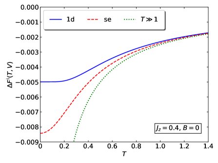
Figure 1: Interaction contribution to the impurity-induced free energy at zero field $\Delta F^{\rm i}(T,V)$ as a function of temperature for the one-dimensional and semi-elliptic density of states for $J_{z}=4V=0.4$. Also included is the large-temperature asymptote (46).

In Fig. 1 we show the interaction contribution to the impurity-induced free energy for zero magnetic field as a function of temperature for the one-dimensional and semi-elliptic density of states. For high temperatures, the free energy becomes independent of the choice of the density of states. It is seen from Fig. 1 that the high-temperature formula (46) becomes applicable for $T\gtrsim 1$.

At $T=0$, the free energy is identical to the ground-state energy, $F(T=0,V)=e_{0}(V)$,

$$e_{0}(V)=\int_{-\infty}^{0}{\rm d}\omega\,\omega\left(D_{0}(\omega,V)+D_{0}(\omega,-V)\right).$$ (50)

From appendix A.2 or, alternatively, from eq. (48) we find the ground-state energy of the Ising-Kondo model

$$e_{0}^{\rm 1d}(V) = 1-\omega_{p}(V)=1-\sqrt{1+V^{2}}$$ (51)

$$\approx -\frac{1}{2}V^{2}\quad\hbox{for}\;V\ll 1$$

for the one-dimensional density of states, and

$$e_{0}^{\rm se}(V) = \frac{1}{\pi}-\frac{1+4V^{2}}{4\pi V}\arctan\left[\frac{4V}{1-4V^{2}}\right]$$ (52)

$$\approx -\frac{8}{3\pi}V^{2}\quad\hbox{for}\;V\ll 1$$

for the semi-elliptic density of states. The ground-state energy for the semi-elliptic density of states is lower than the ground-state energy for the one-dimensional density of states.

As we mentioned earlier, in one dimension only the bound state and the lower band edge contribute to the free energy for low temperatures. Therefore, as a function of temperature, the changes in the interaction contribution to the impurity-induced free energy are exponentially small in $\Delta F^{\rm i}_{\rm 1d}(T,V)$.

In contrast, $\Delta F^{\rm i}_{\rm se}(T,V)$ displays the generic quadratic dependence in $T$ for the semi-elliptic density of states. To make this dependence explicit, we note that the temperature dependence of the free energy in eq. (49) results from the region $|\omega|\lesssim T$. We readily find

$$\Delta F^{\rm i}_{\rm se}(T,V) \approx e_{0}^{\rm se}(V)+F_{2}^{\rm se}(V)T^{2}+{\cal O}(T^{4})\;,$$

$$F_{2}^{\rm se}(V) = \frac{4\pi V^{2}}{3(1+4V^{2})}\;.$$ (53)

Note that $F_{2}^{\rm se}(V)$ is positive for all interaction strengths $V$. This leads to a negative contribution to the specific heat for low temperatures, see Sect. 3.2.4.

3.2.2 Internal energy

We use eq. (25) to calculate the impurity-induced internal energy from the impurity contribution to the free energy. For the one-dimensional density of states we find from eq. (48)

$$U_{\rm 1d}^{\rm i}(T,V)=-\omega_{p}(V)\tanh\left[\frac{\omega_{p}(V)}{2T}\right]+\tanh\left[\frac{1}{2T}\right]$$ (54)

with $\omega_{p}(V)=\sqrt{1+V^{2}}$ for the impurity-induced contribution to the internal energy. For the semi-elliptic density of states, eq. (49) yields

$$U^{\rm i}_{\rm se}(T,V) = -\!\int_{-1}^{1}\frac{{\rm d}\omega}{\pi}\left(\frac{\omega/(2T)}{\cosh^{2}[\omega/(2T)]}+\tanh\Bigl{[}\frac{\omega}{2T}\Bigr{]}\right)$$ (55)

$$\hphantom{-\int_{-1}^{1}\frac{{\rm d}\omega}{\pi}\biggl{[}}\times\arctan\biggl{[}\frac{2V\sqrt{1-\omega^{2}}}{1-2\omega V}\biggr{]}\;.$$

For high temperatures, eq. (46) gives

$$U^{\rm i}(T\gg 1,V)=-\frac{V^{2}}{2T}\;.$$ (56)

This result is independent of the choice of the density of states.

For zero temperature, the internal energy reduces to the ground-state energy, $U^{\rm i}(0,V)=e_{0}(V)$, where the ground-state energy is given in eq. (51) for the one-dimensional density of states (8) and in eq. (52) for the semi-elliptic density of states (10). In one dimension, eq. (54) shows that finite-temperature corrections to the ground-state energy are exponentially small at low temperatures. For the generic semi-elliptic density of states, we find from eq. (53) and eq. (25) that

$$U^{\rm i}_{\rm se}(T,V)\approx e_{0}^{\rm se}(V)-F_{2}^{\rm se}(V)T^{2}+{\cal O}(T^{4})\;.$$ (57)

The impurity contribution to the internal energy decreases as a function of temperature. This again implies that the impurity contribution to the specific heat is negative at low temperatures, see Sect. 3.2.4.

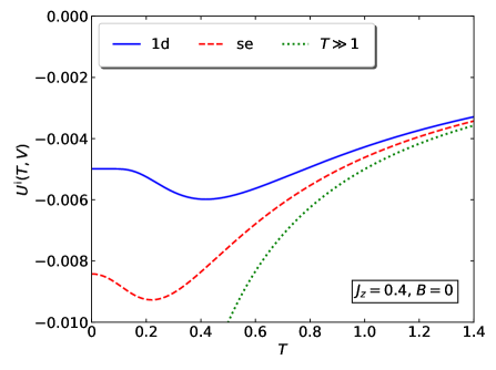
Figure 2: Impurity-induced internal energy at zero field $U^{\rm i}(T,V)$ as a function of temperature for the one-dimensional and semi-elliptic density of states for $J_{z}=4V=0.4$. Also included is the large-temperature asymptote (56).

In Fig. 2 we show the internal energy as a function of temperature for $J_{z}=4V=0.4$ for the one-dimensional and semi-elliptic density of states. Both curves are qualitatively similar. The common high-temperature asymptotic is reached for $T\gtrsim 1.5$ at $J_{z}=0.4$. For small temperatures and in one dimension, the gap for thermal excitations leads to exponentially small changes of the internal energy from the ground-state energy. The semi-elliptic density of states leads to the generic quadratic dependence of the internal energy as a function of temperature for small $T$.

3.2.3 Entropy

The entropy consists of the free impurity contribution $S^{\rm spin}=\ln(2)$ and the interaction-induced impurity terms. Using eq. (26) and eq. (45) we can write

$$S^{\rm i}(T,V)=S^{\rm spin}+\frac{U^{\rm i}(T,V)-\Delta F^{\rm i}(T,V)}{T}\;.$$ (58)

Explicit expressions for $U^{\rm i}(T,V)$ and $\Delta F^{\rm i}(T,V)$ for the one-dimensional density of states are given in eqs. (48) and (54), their counterparts for the semi-elliptic density of states are found in eq. (49) and (55).

For large temperatures, we use the high-temperature limit (56) for $U^{\rm i}(T,V)$ and (46) for $\Delta F^{\rm i}(T,V)$ to determine the limiting behavior of the entropy,

$$S^{\rm i}(T\gg 1,V)\approx\ln(2)-\frac{V^{2}}{4T^{2}}\;;$$ (59)

again, the result is independent of the choice of the density of states. For small temperatures, the interaction-induced contribution to the impurity entropy is exponentially small for the one-dimensional density of states. For the semi-elliptic density of states, we obtain from eq. (53) in eq. (26)

$$S_{\rm se}^{\rm i}(T\ll 1,V)\approx\ln(2)-2F_{2}^{\rm se}(V)T\;,$$ (60)

which displays a linear dependence of the entropy on temperature that is generic for fermionic systems. The negative prefactor shows that the interaction tends to reduce the entropy of the free spin.

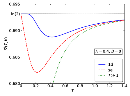
Figure 3: Impurity-induced entropy at zero field $S^{\rm i}(T,V)$ as a function of temperature for the one-dimensional and semi-elliptic density of states for $J_{z}=4V=0.4$. Also included is the large-temperature asymptote (59).

In Fig. 3 we show the impurity entropy. It is seen that the Ising-Kondo interaction decreases the impurity-spin entropy $S^{\rm spin}=\ln(2)$. Note, however, that for small interactions the reduction is small for all temperatures and vanishes for both small and large temperatures. This indicates that screening is not very effective in the Ising-Kondo model. The high-temperature asymptote (59) is reached for $T\gtrsim 1$.

3.2.4 Specific heat

As last point in this subsection, we discuss the specific heat in the absence of a magnetic field. In one dimension, it explicitly reads

$$c_{V}^{\rm i,1d}(T,V) = \frac{[\omega_{p}(V)]^{2}}{2T^{2}\cosh^{2}[\omega_{p}(V)/(2T)]}$$ (61)

$$-\frac{1}{2T^{2}\cosh^{2}[1/(2T)]}$$

with $\omega_{p}(V)=\sqrt{1+V^{2}}$. For the semi-elliptic density of states eq. (55) leads to

$$c_{V}^{\rm i,se}(T,V) = \int_{-1}^{1}{\rm d}\omega\frac{\omega(2T-\omega\tanh[\omega/(2T)])}{2\pi T^{3}\cosh^{2}[\omega/(2T)]}$$ (62)

$$\hphantom{\int_{0}^{1}{\rm d}\omega}\times\arctan\biggl{[}\frac{2V\sqrt{1-\omega^{2}}}{1-2\omega V}\biggr{]}$$

for $V<1/2$. The limit of high temperatures is independent of the choice of the density of states,

$$c_{V}^{\rm i}(T\gg 1,V)\approx\frac{V^{2}}{2T^{2}}\;,$$ (63)

using eq. (56) in eq. (29).

For small temperatures, the specific heat is exponentially small for the one-dimensional density of states. Using eq. (57) in eq. (29) the impurity-induced contribution to the specific heat for the semi-elliptic density of states shows the generic linear dependence on $T$ but with a negative coefficient,

$$c_{V}^{\rm i,se}(T\ll 1,V)\approx-2F_{2}^{\rm se}(V)T$$ (64)

with $F_{2}^{\rm se}(V)$ from eq. (53). Note that the total specific heat of the system remains positive as required for thermodynamic stability since the impurity provides only a small negative contribution.

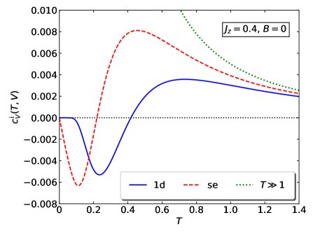
Figure 4: Impurity contribution to the specific heat at zero field $c_{V}^{\rm i}(T,V)$ as a function of temperature for the one-dimensional and semi-elliptic density of states for $J_{z}=4V=0.4$. Also included is the large-temperature asymptote (63).

In Fig. 4 we show the impurity contribution to the specific heat at zero field as a function of temperature for the one-dimensional and semi-elliptic density of states for $J_{z}=4V=0.4$. The specific heat is negative for small temperatures and displays a minimum around $T\lesssim J_{z}/2$ ($T\lesssim J_{z}/4$) and a broad maximum around $T\approx 2J_{z}$ ($T\approx J_{z}$) for the one-dimensional (semi-elliptic) density of states. The high-temperature asymptote (63) becomes applicable for $T\gtrsim 1.5$.

3.3 Thermodynamics at finite magnetic field

As our last subsection, we discuss the thermodynamics at finite magnetic field. While the results are applicable for general $0\leq B<1$, we restrict the discussion to the experimentally realistic region $B\ll V\ll 1$.

3.3.1 Free energy

To address the impurity-induced contribution to the free energy, we abbreviate

$$\bar{F}(B,T,V)=F_{\rm sf}^{\rm i}(B,T,V)+F_{\rm sf}^{\rm i}(-B,T,-V)\;,$$ (65)

where $F_{\rm sf}^{\rm i}(B,T,V)$ is calculated in appendix A.4, so that in eq. (LABEL:eq:fullFimpuritycontribution) we can write

$$F^{\rm i}(B,T,V) = -T\ln\Bigl{[}e^{-\beta[-B+\bar{F}(B,T,V)]}$$ (66)

$$\hphantom{-T\ln\Bigl{[}}+e^{-\beta[B+\bar{F}(-B,T,V)]}\Bigr{]}\;.$$

We split $\bar{F}(B,T,V)=\bar{F}_{\rm s}(B,T,V)+\bar{F}_{\rm a}(B,T,V)$ into two parts that are symmetric and antisymmetric in $B$,

$$\bar{F}_{\rm s}(-B,T,V) = \bar{F}_{\rm s}(B,T,V)\;,$$

$$\bar{F}_{\rm a}(-B,T,V) = -\bar{F}_{\rm a}(B,T,V)\;,$$ (67)

and find in eq. (66)

$$F^{\rm i}(B,T,V) = \bar{F}_{\rm s}(B,T,V)$$ (68)

$$-T\ln\left[2\cosh[B^{\rm eff}(B,T,V)/T]\right]\,,$$

$$B^{\rm eff}(B,T,V) = B-\bar{F}_{\rm a}(B,T,V)\;.$$ (69)

For small fields we have

$$\bar{F}_{\rm s}(B\ll 1,T,V) = F^{\rm i}(T,V)+{\cal O}(B^{2})\;,$$

$$\bar{F}_{\rm a}(B\ll 1,T,V) = \alpha(T,V)B+{\cal O}(B^{3})\;,$$

$$\alpha(T,V) = \left.\frac{\partial\bar{F}(B,T,V)}{\partial B}\right|_{B=0}$$ (70)

so that, in the small-field limit,

$$B^{\rm eff}(B\ll 1,T,V) = \left(1-\alpha(T,V)\right)B\;,$$

$$F^{\rm i}(B\ll 1,T,V) \approx F^{\rm i}(T,V)$$

$$-T\ln\biggl{[}2\cosh\Bigl{[}\frac{(1-\alpha(T,V))B}{T}\Bigr{]}\biggr{]}.$$

For a free spin we obtain

$$F^{\rm spin}(B,T)=-T\ln\biggl{[}2\cosh\Bigl{[}\frac{B}{T}\Bigr{]}\biggr{]}\;.$$ (72)

A comparison with eq. (LABEL:eq:FilowTsecondstepgeneralsmallB) shows that, for small external fields, the impurity-contribution to the free energy consists of the field-free term discussed in Sect. 3.2 and the contribution of a free spin in the effective field $B^{\rm eff}(B,T,V)=(1-\alpha(T,V))B$.

To present tangible results, we use the one-dimensional host-electron density of states in eq. (3.1.2) and the semi-elliptic host-electron density of states in eq. (41) when $V<1/2$ to evaluate the free energy for spinless fermions from eq. (39). Performing a partial integration we can write ($F^{\rm 1d,se}_{\rm s,a}\equiv F^{\rm 1d,se}_{\rm s,a}(B,T,V)$, $\omega_{p}(V)=\sqrt{1+V^{2}}$)

$$\bar{F}^{\rm 1d}_{\rm s}=-T\ln\left[\frac{\cosh(B/T)+\cosh(\omega_{p}(V)/T)}{\cosh(B/T)+\cosh(1/T)}\right]\;,$$ (73)

compare eq. (48), and

$$\bar{F}^{\rm 1d}_{\rm a} = \int_{-1}^{1}\frac{{\rm d}\omega}{\pi}\arctan\left[\frac{V}{\sqrt{1-\omega^{2}}}\right]$$ (74)

$$\hphantom{\int_{-1}^{1}\frac{{\rm d}\omega}{\pi}}\left(\frac{1}{1+e^{(\omega-B)/T}}-\frac{1}{1+e^{(\omega+B)/T}}\right)\,.$$

Moreover,

$$\bar{F}^{\rm se}_{\rm s} = -\int_{-1}^{1}\frac{{\rm d}\omega}{2\pi}\left(\tanh\left[\frac{\omega-B}{2T}\right]+\tanh\left[\frac{\omega+B}{2T}\right]\right)$$ (75)

$$\hphantom{-\int_{-1}^{1}\frac{{\rm d}\omega}{2\pi}}\times\arctan\biggl{[}\frac{2V\sqrt{1-\omega^{2}}}{1-2\omega V}\biggr{]}\,,$$

compare eq. (49), and

$$\bar{F}^{\rm se}_{\rm a} = -\int_{-1}^{1}\frac{{\rm d}\omega}{2\pi}\left(\tanh\left[\frac{\omega-B}{2T}\right]-\tanh\left[\frac{\omega+B}{2T}\right]\right)$$ (76)

$$\hphantom{-\int_{-1}^{1}\frac{{\rm d}\omega}{2\pi}}\times\arctan\biggl{[}\frac{2V\sqrt{1-\omega^{2}}}{1-2\omega V}\biggr{]}\,.$$

We again split the impurity free energy into the interaction contributions and that of the free spin,

$$\Delta F^{\rm i}(B,T,V)=F^{\rm i}(B,T,V)-F^{\rm spin}(B,T)$$ (77)

with $F^{\rm spin}(B,T)$ from eq. (72) so that $\Delta F^{\rm i}(B,T,V=0)=0$ for all fields and temperatures.

Simplifications of the above expressions are only possible in limiting cases. For high temperatures, $T\gg 1$, we expand

$$-\beta F_{\rm sf}^{\rm i}(B,T\gg 1,V) \approx -\frac{1}{2T}\omega_{1}(V)$$

$$+\frac{1}{8T^{2}}\left(\omega_{2}(V)-2B\omega_{1}(V)\right)\;,$$

$$\omega_{n} = \int_{-\infty}^{\infty}{\rm d}\omega\,\omega^{n}D_{0}(\omega,V)\;.$$ (78)

Note that $\omega_{n}(-V)=(-1)^{n}\omega_{n}(V)$ due to the symmetry $D_{0}(\omega,-V)=D_{0}(-\omega,V)$. Then, we obtain

$$F^{\rm spin}(B,T\gg 1) \approx -T\ln(2)-\frac{B^{2}}{2T}\;,$$

$$\Delta F^{\rm i}(B,T\gg 1,V) \approx -\frac{\omega_{2}(V)}{4T}+\frac{\omega_{1}(V)B^{2}}{2T^{2}}\;,$$ (79)

with corrections of the order $1/T^{3}$. Using Mathematica [19] we find $\omega_{1}(V)=V$ and $\omega_{2}(V)=V^{2}$ so that for $T\gg 1$

$$\Delta F^{\rm i}(B,T\gg 1,V)\approx-\frac{V^{2}}{4T}+\frac{VB^{2}}{2T^{2}}\;,$$ (80)

up to and including second order in $1/T$. Using perturbation theory in $J_{z}/T$ [7, 15], it is readily shown that $\Delta F^{\rm i}(B,T,V)$ is indeed independent of the host-electron density of states up to second order in $J_{z}/T$. Eqs. (79) and (80) show that small magnetic fields induce small corrections, of the order $B^{2}$.

At low temperatures, eq. (LABEL:eq:FilowTsecondstepgeneralsmallB) shows that the temperature dependence of the impurity contribution to the free energy is dominated by the logarithm. Therefore, the Sommerfeld expansion of $\bar{F}(T,V)$ [2, 18] can be restricted to the leading-order term, i.e., we use $\bar{F}(B,T\ll 1,V)\approx\bar{F}(B,T=0,V)\equiv\bar{E}(B,V)$. Thus, we find in eq. (68)

$$F^{\rm i}(B,T\ll 1,V) \approx \bar{E}_{\rm s}(B,V)$$ (81)

$$-T\ln\left[2\cosh[B^{\rm eff}(B,V)/T]\right]\,,$$

$$B^{\rm eff}(B,V) = B-\bar{E}_{\rm a}(B,V)$$ (82)

with $B^{\rm eff}(B,V)\equiv B^{\rm eff}(B,T=0,V)$. Eq. (81) shows that the low-temperature thermodynamics of the model at finite fields is described by a free spin in an effective field $B^{\rm eff}(B,V)$. Eq. (81) is actually applicable in the temperature region $T\lesssim B^{\rm eff}(B,V)$. At low temperatures, the interaction-induced impurity contribution to the free energy becomes

$$\Delta F^{\rm i}(T\ll 1) \approx \bar{E}_{\rm s}(B,V)$$

$$-T\ln\left[\frac{\cosh[(B-\bar{E}_{\rm a}(B,V))/T]}{\cosh[B/T]}\right]\;,$$

where we abbreviate $\Delta F^{\rm i}(T\ll 1)\equiv\Delta F^{\rm i}(B,T\ll 1,V)$.

The above expressions can be worked out further when the density of states is specified. For the one-dimensional density of states we have

$$\bar{E}^{\rm 1d}_{\rm s}(B,V) = e_{0}^{\rm 1d}(V)=1-\omega_{p}(V)=1-\sqrt{1+V^{2}}\;,$$

$$\bar{E}^{\rm 1d}_{\rm a}(B,V) = \int_{-B}^{B}\frac{{\rm d}\omega}{\pi}\arctan\left[\frac{V}{\sqrt{1-\omega^{2}}}\right]$$ (84)

with $e_{0}^{\rm 1d}(V)$ from eq. (51), and, with $\omega_{p}(V)=\sqrt{1+V^{2}}$,

$$\bar{E}^{\rm 1d}_{\rm a}(B,V) = \frac{2V}{\pi}\arcsin(B)+\frac{2B}{\pi}\arctan\left[\frac{V}{\sqrt{1-B^{2}}}\right]$$ (85)

$$-\frac{2\omega_{p}(V)}{\pi}\arctan\biggl{[}\frac{BV}{\omega_{p}(V)\sqrt{1-B^{2}}}\biggr{]}\;,$$

where we used Mathematica [19] to carry out the integral.

For the semi-elliptic density of states we find

$$\bar{E}^{\rm se}_{\rm s}(B,V) = \int_{-1}^{-B}\frac{{\rm d}\omega}{\pi}\arctan\left[\frac{2V\sqrt{1-\omega^{2}}}{1-2\omega V}\right]$$ (86)

$$-\int_{B}^{1}\frac{{\rm d}\omega}{\pi}\arctan\left[\frac{2V\sqrt{1-\omega^{2}}}{1-2\omega V}\right]$$

and

$$\bar{E}^{\rm se}_{\rm a}(B,V)=\int_{-B}^{B}\frac{{\rm d}\omega}{\pi}\arctan\left[\frac{2V\sqrt{1-\omega^{2}}}{1-2\omega V}\right]\;.$$ (87)

With $\bar{\omega}(V)=\sqrt{1+4V^{2}}$ we explicitly have

$$\bar{E}^{\rm se}_{\rm s}(B,V) = \frac{\sqrt{1-B^{2}}}{\pi}\;$$

$$+\frac{B}{\pi}\arctan\left[\frac{2V\sqrt{1-B^{2}}}{1-2BV}\right]$$

$$-\frac{B}{\pi}\arctan\left[\frac{2V\sqrt{1-B^{2}}}{1+2BV}\right]$$

$$+\frac{\bar{\omega}^{2}(V)}{8\pi V}\arctan\left[\frac{B\bar{\omega}^{2}(V)-4V}{\sqrt{1-B^{2}}(1-4V^{2})}\right]$$

$$-\frac{\bar{\omega}^{2}(V)}{8\pi V}\arctan\left[\frac{B\bar{\omega}^{2}(V)+4V}{\sqrt{1-B^{2}}(1-4V^{2})}\right]$$

and

$$\bar{E}^{\rm se}_{\rm a}(B,V) = -\frac{(1-4V^{2})\arcsin(B)}{4\pi V}$$

$$+\frac{B}{\pi}\arctan\left[\frac{2V\sqrt{1-B^{2}}}{1-2BV}\right]$$

$$+\frac{B}{\pi}\arctan\left[\frac{2V\sqrt{1-B^{2}}}{1+2BV}\right]$$

$$+\frac{\bar{\omega}^{2}(V)}{8\pi V}\arctan\left[\frac{B\bar{\omega}^{2}(V)-4V}{\sqrt{1-B^{2}}(1-4V^{2})}\right]$$

$$+\frac{\bar{\omega}^{2}(V)}{8\pi V}\arctan\left[\frac{B\bar{\omega}^{2}(V)+4V}{\sqrt{1-B^{2}}(1-4V^{2})}\right]\;,$$

where we used Mathematica [19] to carry out the integrals.

At $T=0$, the impurity-contribution to the ground-state energy is obtained from eq. (81) as

$$e_{0}(B,V)=\bar{E}_{\rm s}(B,V)-|B-\bar{E}_{a}(B,V)|\;.$$ (90)

The absolute value can be ignored because the argument is always positive for $B>0$. Thus, we have

$$e_{0}(B,V) \equiv F^{\rm i}(B,T=0,V)$$ (91)

$$= \bar{E}_{\rm s}(B,V)+\bar{E}_{a}(B,V)-B$$

for the interaction contribution to the impurity-induced change in the ground-state energy at finite fields $B$.

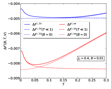
Figure 5: Interaction contribution to the impurity-induced free energy $\Delta F^{\rm i}(B,T,V)$ as a function of temperature for the one-dimensional and semi-elliptic density of states for $B=0.01$ and $J_{z}=4V=0.4$. Also included is the free energy at zero field, eqs. (48) and (49), and the low-temperature approximation (LABEL:eq:DeltaFi).

In Fig. 5 we show the interaction contribution to the impurity-induced free energy $\Delta F^{\rm i}(B,T,V)$ as a function of temperature for the one-dimensional and semi-elliptic density of states for $B=0.01$ and $J_{z}=4V=0.4$. The low-temperature expression (LABEL:eq:DeltaFi) works very well until $\Delta F^{\rm i}(B,T,V)$ reaches its limiting value $\Delta F^{\rm i}(B,T\gg B,V)=\bar{E}_{\rm s}(B,V)$ for $T\gtrsim 2B^{\rm eff}$. Thus, it is clearly seen that, at very low temperatures $T\lesssim B\ll 1$, the thermodynamics of the Ising-Kondo model can be described by a spin-1/2 in an effective field, see eq. (82). In the region $T\gtrsim V$, a small magnetic field becomes irrelevant and we may approximate $\Delta F^{\rm i}(B\ll 1,T\gtrsim B,V)\approx\Delta F^{\rm i}(B=0,T,V)$.

For further reference, we list the results in the limit of small fields. We have

$$\bar{E}^{\rm 1d}_{\rm a}(B,V) \approx \frac{2B}{\pi}\arctan(V)+\frac{B^{3}}{3\pi}\frac{V}{1+V^{2}}+{\cal O}(B^{5})\;,$$

$$\bar{E}^{\rm se}_{\rm s}(B,V) \approx e_{0}^{\rm se}(V)+\frac{4B^{2}}{\pi}\frac{V^{2}}{1+4V^{2}}+{\cal O}(B^{4})\;,$$

$$\bar{E}^{\rm se}_{\rm a}(B,V) \approx \frac{2B}{\pi}\arctan(2V)-\frac{2B^{3}}{3\pi}\frac{1-4V^{2}}{(1+4V^{2})^{2}}$$ (92)

$$+{\cal O}(B^{5})$$

for $B\ll 1$ with $e_{0}^{\rm se}(V)$ from eq. (52). Moreover, for the ground-state energy we find

$$e_{0}^{\rm 1d}(B\ll 1,V) \approx e_{0}^{\rm 1d}(V)-B\left(1-\frac{2}{\pi}\arctan(V)\right)\;,$$

$$e_{0}^{\rm se}(B\ll 1,V) \approx e_{0}^{\rm se}(V)+\frac{4B^{2}}{\pi}\frac{V^{2}}{1+4V^{2}}$$ (93)

$$-B\left(1-\frac{2}{\pi}\arctan(2V)\right)\;,$$

up to and including second order in $B>0$ with $e_{0}^{\rm 1d}(V)$ from eq. (51) and $e_{0}^{\rm se}(V)$ from eq. (52).

For small fields, the effective field in eq. (82) is scaled linearly, see eqs. (70) and (LABEL:eq:FilowTsecondstepgeneralsmallB) with $\alpha(V)\equiv\alpha(T=0,V)$,

$$B^{\rm eff}(B,V) \approx (1-\alpha(V))B\;,$$

$$\alpha^{\rm 1d}(V) = \frac{2}{\pi}\arctan(V)\;,$$

$$\alpha^{\rm se}(V) = \frac{2}{\pi}\arctan(2V)\;.$$ (94)

For small interactions, the effect is small, of the order $V$. Due to the interaction, the effective magnetic field is somewhat smaller than the external field. This is readily understood from the fact that the conduction electrons screen the impurity and thus weaken the externally applied field.

3.3.2 Internal energy and entropy

Next, we briefly discuss the impurity-induced internal energy and entropy for the case of small fields.

For all temperatures, couplings, and fields, the internal energy and the entropy are obtained from the free energy by differentiation with respect to $T$, see eq. (25) for the internal energy and eq. (26) for the entropy. Since we assume a small magnetic field, typically $B\ll J_{z}\ll 1$, the impurity-induced internal energy and entropy follow the curves shown in Fig. 2 and Fig. 3 when $T\gtrsim V$, with small corrections of the order $B^{2}$.

For small temperatures, $T\lesssim B$, we start from eq. (LABEL:eq:DeltaFi) and find for the internal energy of a spin in an effective field

$$U^{\rm i}(B,T\lesssim B,V) = \bar{E}_{\rm s}(B,V)$$

$$-B^{\rm eff}(B,V)\tanh\left[\frac{B^{\rm eff}(B,V)}{T}\right]$$

with $B^{\rm eff}(B,V)$ from eq. (82). The impurity-contribution to the entropy reads

$$S^{\rm i}(B,T\lesssim B,V) = \ln\left[2\cosh(B^{\rm eff}(B,V)/T)\right]$$

$$-\frac{B^{\rm eff}(B,V)}{T}\tanh\left[\frac{B^{\rm eff}(B,V)}{T}\right]$$

for low temperatures; for a free spin, replace $B^{\rm eff}$ by $B$ in eqs. (3.3.2) and (3.3.2).

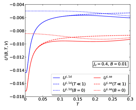
Figure 6: Impurity-induced internal energy $U^{\rm i}(B,T,V)$ as a function of temperature for the one-dimensional and semi-elliptic density of states for $J_{z}=4V=0.4$ and external field $B=0.01$. Also included is the low-temperature approximation (3.3.2) and the zero-field approximation shown in Fig. 2.

Figure 7: Impurity-induced entropy $S^{\rm i}(B,T,V)$ as a function of temperature for the one-dimensional and semi-elliptic density of states for $J_{z}=4V=0.4$ and external field $B=0.01$. Also included is the low-temperature approximation (3.3.2) and the zero-field approximation shown in Fig. 3.

In Fig. 6 we show the impurity-induced internal energy $U^{\rm i}(B,T,V)$ as a function of temperature for the one-dimensional and semi-elliptic density of states for $J_{z}=4V=0.4$, a small external field $B=0.01$, and low temperatures. The internal energy increases from its value $e_{0}(B,V)$, eq. (91), only exponentially slowly because the magnetic field induces an energy gap of the order $B^{\rm eff}(B,V)$ between the two spin orientations.

When the temperature becomes of the order of the effective magnetic field $B^{\rm eff}(B,V)$, the impurity contribution to the internal energy $U^{\rm i}(B,T,V)$ approaches the value $\bar{E}_{\rm s}(B,V)\approx e_{0}(V)$, with corrections of the order $B^{2}$, and the approximate low-temperature internal energy (3.3.2) starts to deviate from the exact result. At temperatures $T\gtrsim V$, the internal energy becomes essentially identical to its zero-field value shown in Fig. 2 on a larger temperature scale.

In Fig. 7 we show the impurity contribution to the entropy $S^{\rm i}(B,T,V)$ as a function of temperature for the one-dimensional and semi-elliptic density of states for $J_{z}=4V=0.4$, and a small external field $B=0.01$. In contrast to the zero-field case, the entropy is zero at zero temperature because the impurity spin is oriented along the effective external field. Due to the excitation gap, the entropy is exponentially small for $T\ll B^{\rm eff}(B,V)$. When the temperature becomes of the order of $B^{\rm eff}(B,V)$, the impurity entropy approaches $S\approx\ln(2)$. For $T\gtrsim V$, it becomes essentially identical to its zero-field value shown in Fig. 3 on a larger temperature scale.

3.3.3 Magnetization and impurity spin polarization

For the calculation of the impurity-induced magnetization $m^{\rm i}(B,T,V)\equiv m^{\rm i}$, see eq. (2.2.3), we start from eq. (68) and find

$$m^{\rm i}=-\frac{1}{2}\left[\frac{\partial\bar{F}_{\rm s}}{\partial B}-\left(1-\frac{\partial\bar{F}_{\rm a}}{\partial B}\right)\tanh\left[\frac{B-\bar{F}_{\rm a}}{T}\right]\right]$$ (97)

with $\bar{F}_{\rm s/a}\equiv\bar{F}_{\rm s/a}(B,T,V)$. We numerically perform the derivatives with respect to $B$ for all temperatures.

At temperature $T=0$, eq. (91) gives for $B>0$

$$m^{\rm i}(B,V) \equiv m^{\rm i}(B,0,V)\;,$$

$$m^{\rm i}(B,V) = \frac{1}{2}\left(1-\frac{\partial\bar{E}_{\rm s}(B,V)}{\partial B}-\frac{\partial\bar{E}_{\rm a}(B,V)}{\partial B}\right)\;.$$ (98)

For the model density of states we obtain

$$m^{\rm i,1d}(B,V) = \frac{1}{2}-\frac{1}{\pi}\arctan\left[\frac{V}{\sqrt{1-B^{2}}}\right]\;,$$

$$m^{\rm i,se}(B,V) = \frac{1}{2}-\frac{1}{\pi}\arctan\left[\frac{2V\sqrt{1-B^{2}}}{1-2BV}\right]\;.$$ (99)

At $V=0$, we recover the value for a free spin in a finite field at zero temperature, $m^{\rm i}(B>0,T=0,V=0)=m^{\rm spin}(B>0,T=0)=1/2$. For finite antiferromagnetic interactions, $V>0$, the impurity-induced magnetization is smaller than the free-spin value because the impurity spin is screened by the band electrons in its surrounding, see Sect. 4.

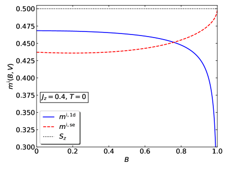
Figure 8: Impurity-induced magnetization at zero temperature $m^{\rm i}(B,T=0,V)$ as a function of magnetic field for the one-dimensional and semi-elliptic density of states for $J_{z}=4V=0.4$ from eq. (99). Also included is the value for the impurity spin polarization, $S_{z}(B>0,T=0,V)=1/2$ from eq. (104).

In Fig. 8 we show the impurity-induced magnetization at zero temperature $m^{\rm i}(B,V)\equiv m^{\rm i}(B,T=0,V)$ as a function of magnetic field for the one-dimensional and semi-elliptic density of states for $J_{z}=4V=0.4$. Due to the larger density of states at the Fermi energy for small $B$, the screening is more effective for the semi-elliptic density of states than for the one-dimensional density of states. Since the one-dimensional density of states diverges at the band edges, the two curves cross at some (very large) magnetic fields, $B\approx 0.8$. At $B=1$, the screening vanishes for the semi-elliptic density of states, $m^{\rm i,se}(B=1,T=0,V)=1/2$, and becomes perfect for the one-dimensional density of states, $m^{\rm i,1d}(B=1,T=0,V)=0$, reflecting the behavior of the density of states at the band edges.

For low temperatures, $T\lesssim B$, the asymptotic expression for the magnetization is obtained from eq. (97) as

$$m^{\rm i}(B,T\lesssim B,V) \approx -\frac{1}{2}\frac{\partial\bar{E}_{\rm s}}{\partial B}$$

$$+\frac{1}{2}\Bigl{(}1-\frac{\partial\bar{E}_{\rm a}}{\partial B}\Bigr{)}\tanh\biggl{[}\frac{B^{\rm eff}(B,V)}{T}\biggr{]}$$

with $B^{\rm eff}(B,V)$ from eq. (82). For small fields this can be further simplified to give

$$m^{\rm i}(B\ll 1,T\ll 1,V)\approx\!\frac{B^{\rm eff}(B,V)}{2B}\tanh\biggl{[}\frac{B^{\rm eff}(B,V)}{T}\biggr{]}$$ (101)

with $B^{\rm eff}(B,V)/B=1-\alpha(V)$ from eq. (94). This shows that, for small fields and temperatures, the magnetization is a universal function of $B/T$, as for a free spin [2, 18].

For high temperatures, we can derive the asymptote from eqs. (79) and (80) as

$$m^{\rm i}(B,T\gg 1)\approx\frac{B}{2T}\left(1-\frac{V}{T}\right)\;,$$ (102)

with corrections of the order $1/T^{3}$.

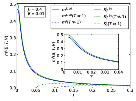
Figure 9: Impurity-induced magnetization $m^{\rm i}(B,T,V)$ and impurity spin polarization $S_{z}(B,T,V)$ as a function of temperature for the one-dimensional density of states for $J_{z}=4V=0.4$ and external field $B=0.01$. Also included are the approximate results for low temperatures and small fields from eq. (101) and eq. (104), respectively, and the large-temperature asymptotes, eq. (102) and eq. (105). Inset: region of small temperatures.

In Fig. 9 we show the impurity-induced magnetization $m^{\rm i}(B,T,V)$ as a function of temperature for the one-dimensional of states for $J_{z}=4V=0.4$ and $B=0.01$; the curves for the semi-elliptic density of states are qualitatively very similar. For small interactions, the temperature-dependence of the magnetization follows that of a free spin in an effective field, i.e., the temperature dependence is very small as long as $T\lesssim B^{\rm eff}(B,V)$, see eq. (LABEL:eq:magsmallTapprox). When $T$ exceeds $B^{\rm eff}$ the magnetization rapidly declines and approaches zero for high temperatures. Indeed, as seen from eq. (102), at large temperatures the magnetization vanishes proportional to $1/T$, as for a free spin; interaction corrections are smaller, of the order $V/T^{2}$.

To demonstrate the screening of the host electrons, we compare the impurity-induced magnetization with the impurity spin polarization. We have from eq. (28)

$$S_{z} = \frac{1}{2}\frac{e^{-\beta[-B+\bar{F}(B,T,V)]}-e^{-\beta[B-\bar{F}(-B,T,V)]}}{e^{-\beta[-B+\bar{F}(B,T,V)]}+e^{-\beta[B-\bar{F}(-B,T,V)]}}$$ (103)

$$= \frac{1}{2}\tanh\left[\frac{B^{\rm eff}(B,T,V)}{T}\right]$$

with $S_{z}\equiv S_{z}(B,T,V)$ and $B^{\rm eff}(B,T,V)$ from eq. (LABEL:eq:FilowTsecondstepgeneralsmallB).

For low temperatures and $B>0$, this expression simplifies to

$$S_{z}(B,T\lesssim B,V)\approx\frac{1}{2}\tanh\left[\frac{B^{\rm eff}(B,V)}{T}\right]$$ (104)

with $B^{\rm eff}(B,V)$ from eq. (82). For $T=0$ and $B>0$, the impurity spin is aligned with the external field. A comparison with eq. (101) shows that, at low temperatures and small fields, the impurity spin polarization and the impurity-induced magnetization differ by a factor $B^{\rm eff}(B,V)/B=1-\alpha(V)$. The impurity-induced magnetization is smaller because it is more sensitive to the screening by the host electrons.

For large temperatures, we find from eq. (78)

$$S_{z}(B,T\gg 1,V)\approx\frac{B}{2T}\left(1-\frac{V}{2T}\right)$$ (105)

with corrections of the order $T^{-3}$. The impurity-induced magnetization and the impurity spin polarization agree to first order in $1/T$ (free spin) but slightly differ already in second order, compare eq. (102) and eq. (105). Again, the impurity-induced magnetization is smaller than the impurity spin polarization because of the larger screening contribution from the host electrons. The results for the impurity spin polarization are visualized in Fig. 9 in comparison with those for the impurity-induced magnetization. For small fields and interactions, the differences between $m^{\rm i}$ and $S_{z}$ are small but discernible.

3.3.4 Response functions

Lastly, we discuss the specific heat in the presence of a small magnetic field and the zero-field susceptibilities for the impurity-induced magnetization and the impurity spin polarization.

In general, we calculate the specific heat from the internal energy using eq. (29), see eqs. (61) and (62) for the zero-field case and the two model density of states. For small $B$, we thus focus on small temperatures where we can use eq. (3.3.2) to find

$$c_{V}^{\rm i}(B,T\lesssim B,V)\approx\left(\frac{B^{\rm eff}(B,V)}{T\cosh[B^{\rm eff}(B,V)/T]}\right)^{2}$$ (106)

with $B^{\rm eff}(B,V)$ from eq. (82). It is seen that the specific heat displays a peak around $B^{\rm eff}(B,V)$. Due to the screening by the host electrons, the impurity spin in the Ising-Kondo model behaves like a free spin in an effective field.

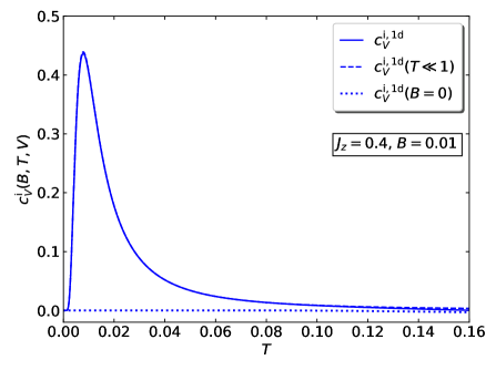
Figure 10: Impurity contribution to the specific heat $c_{V}^{\rm i}(B,T,V)$ as a function of temperature for the one-dimensional density of states for $J_{z}=4V=0.4$ and $B=0.01$. Also included is the specific heat for zero field from eq. (61) as shown in Fig. 4 on a larger temperature scale.

We show the specific heat in Fig. 10 for $J_{z}=4V=0.4$ and $B=0.01$ as a function of temperature for the one-dimensional density of states; the curves for the semi-elliptic density of states differ only slightly. For small fields, the specific heat approaches the zero-field value around $T\gtrsim V$, with small corrections of the order $B^{2}$.

Lastly, we consider the zero-field susceptibilities at finite temperature $T>B=0$. Since we keep $T$ finite and let $B$ go to zero first, none of the approximate expressions is applicable that were derived for the impurity-induced magnetization or the impurity spin polarization in Sect. 3.3.3.

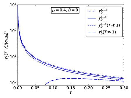
Figure 11: Impurity contribution to the zero-field magnetic susceptibilities $\chi_{0}^{\rm i(S)}(T,V)$ as a function of temperature for the one-dimensional density of states for $J_{z}=4V=0.4$. Also included are the asymptotic expressions for $\chi_{0}^{\rm i}(T,V)$, eq. (110) for high temperatures and eq. (111) for low temperatures. Note the logarithmic scale on the ordinate.

Using the impurity-induced free energy (LABEL:eq:FilowTsecondstepgeneralsmallB) we can derive the zero-field susceptibility as

$$\frac{\chi_{0}^{\rm i}(T,V)}{(g_{e}\mu_{\rm B})^{2}}=\frac{1}{4T}\left(1-\alpha(T,V)\right)^{2}\;,$$ (107)

see eq. (70). Explicitly, for the one-dimensional density of states we have

$$\alpha_{\rm 1d}(T,V) = \tanh\left[\frac{\sqrt{1+V^{2}}}{2T}\right]-\tanh\left[\frac{1}{2T}\right]$$ (108)

$$+\frac{2}{T}\int_{-1}^{1}\frac{{\rm d}\omega}{\pi}\left(\frac{1}{2\cosh[\omega/(2T)]}\right)^{2}$$

$$\hphantom{+\frac{2}{T}\int_{-1}^{1}}\times\arctan\left[\frac{V}{\sqrt{1-\omega^{2}}}\right],$$

and for the semi-elliptic density of states we find

$$\alpha_{\rm se}(T,V) = \frac{2}{T}\int_{-1}^{1}\frac{{\rm d}\omega}{\pi}\left(\frac{1}{2\cosh[\omega/(2T)]}\right)^{2}$$ (109)

$$\hphantom{\frac{2}{T}\int_{-1}^{1}}\times\arctan\left[\frac{2V\sqrt{1-\omega^{2}}}{1-2\omega V}\right].$$

For high temperatures, this gives

$$\frac{\chi_{0}^{\rm i}(T\gg 1,V)}{(g_{e}\mu_{\rm B})^{2}}=\frac{1}{4T}\left(1-\frac{V}{2T}\right)^{2}+{\cal O}(T^{-4})\;.$$ (110)

for a general density of states. For small temperatures we find

$$\frac{\chi_{0}^{\rm i}(T\ll 1,V)}{(g_{e}\mu_{\rm B})^{2}}=\frac{1}{4T}\left(1-\alpha(V)\right)^{2}\equiv\frac{\tilde{C}}{T}\;,$$ (111)

where $1-\alpha(V)$ is the reduction factor for the magnetic field for small fields at zero temperature, see eq. (94). This had to be expected because, for small fields and low temperatures, the system describes an impurity spin in an effective field. Therefore, we obtain the Curie law (111) with a modified Curie constant $\tilde{C}$ [2, 18].

In Fig. 11 we show the impurity-induced zero-field magnetic susceptibility $\chi_{0}^{\rm i}(T,V)$ as a function of temperature for the one-dimensional density of states for $V=0.1$ ($J_{z}=0.4$); the curves for the semi-elliptic density of states are almost identical. The high-temperature asymptote (110) and the low-temperature asymptote (111) together provide a very good description of the zero-field impurity-induced magnetic susceptibility.

Since the Curie constant is proportional to $S(S+1)/3$ with $S=1/2$ in our case, we can argue that the Ising-Kondo interaction with the host electrons reduces the effective spin on the impurity,

$$S^{\rm eff}(V) = \frac{1}{2}-\left(1-\sqrt{1-\frac{3\alpha(V)}{2}+\frac{3\alpha^{2}(V)}{4}}\right)$$ (112)

$$\approx \frac{1}{2}-\frac{3\alpha(V)}{4}\quad\hbox{for $\alpha\ll 1$.}$$

It is only for $V=\infty$ that $\alpha(V)=1$, i.e., there always remains an unscreened spin on the impurity.

Finally, we address the spin impurity susceptibility,

$$\frac{\chi_{0}^{\rm i,S}(T,V)}{(g_{e}\mu_{\rm B})^{2}}=\frac{1}{4T}\left(1-\alpha(T,V)\right)\;,$$ (113)

where we took the derivative of $S_{z}(B,T,V)$ in eq. (103) with respect to $B$ and put $B=0$ afterwards. The impurity spin susceptibility is also reduced from its free-spin value but the reduction factor is only linear in $(1-\alpha(T,V))$ instead of quadratic as for the impurity-induced magnetic susceptibility, see eq. (107). Fig. 11 also shows the impurity spin susceptibility as a function of temperature for $J_{z}=4V=0.4$.

4 Screening cloud

In this section we first calculate the matrix element for the spin correlation between impurity and bath electrons. Next, we focus on the spin correlation function on a chain. Lastly, we discuss the screening cloud in one spatial dimension.

4.1 Spin correlation function

We evaluate the spin correlation function (33). At $B=0$, the partition function is given by

$${\cal Z}_{\rm IK}(\beta,V)=2\bar{Z}_{\rm sf}(\beta,V)\bar{Z}_{\rm sf}(\beta,-V)$$ (114)

with $\bar{Z}_{\rm sf}(\beta,V)\equiv\bar{Z}_{\rm sf}(\beta,B=0,V)$ and $V=J_{z}/4>0$ because, in the absence of a magnetic field, the two impurity orientations contribute equally and the bath electrons experience either a repulsive or an attractive potential at the origin. Then,

$$C_{dc}^{S}(r) = \frac{1}{2{\cal Z}}\langle\Uparrow\!|\mathop{\rm Tr}\nolimits_{c}\biggl{[}e^{-\beta[\hat{T}+V(\hat{n}_{\Uparrow}^{d}-\hat{n}_{\Downarrow}^{d})(\hat{c}_{0,\uparrow}^{+}\hat{c}_{0,\uparrow}^{\vphantom{+}}-\hat{c}_{0,\downarrow}^{+}\hat{c}_{0,\downarrow}^{\vphantom{+}})]}$$

$$\hphantom{\frac{1}{4{\cal Z}}\langle\Uparrow\!|}\times\left(\hat{n}_{\Uparrow}^{d}-\hat{n}_{\Downarrow}^{d}\right)\Bigl{(}\hat{n}_{r,\uparrow}-\hat{n}_{r,\downarrow}\Bigr{)}\biggr{]}|\!\Uparrow\rangle$$

because the impurity spin configuration $|\!\Downarrow\rangle$ gives the same contribution due to spin symmetry. At half band-filling, $\mu(T,V)=0$ for all temperatures $T$ and interaction strengths $V$, see eq. (21).

Since $\hat{n}_{\Uparrow}^{d}|\!\Uparrow\rangle=|\!\Uparrow\rangle$ and $\hat{n}_{\Downarrow}^{d}|\!\Uparrow\rangle=0$, we find

$$C_{dc}^{S}(r) = \frac{1}{2{\cal Z}}\mathop{\rm Tr}\nolimits_{c,\uparrow}\biggl{[}e^{-\beta[\hat{T}_{\uparrow}+V\hat{c}_{0,\uparrow}^{+}\hat{c}_{0,\uparrow}^{\vphantom{+}}]}\hat{c}_{r,\uparrow}^{+}\hat{c}_{r,\uparrow}^{\vphantom{+}}\biggr{]}$$ (116)

$$\hphantom{\frac{1}{2{\cal Z}}}\times\mathop{\rm Tr}\nolimits_{c,\downarrow}\biggl{[}e^{-\beta[\hat{T}_{\downarrow}-V\hat{c}_{0,\downarrow}^{+}\hat{c}_{0,\downarrow}^{\vphantom{+}}]}\biggr{]}$$

$$-\frac{1}{2{\cal Z}}\mathop{\rm Tr}\nolimits_{c,\uparrow}\biggl{[}e^{-\beta[\hat{T}_{\uparrow}+V\hat{c}_{0,\uparrow}^{+}\hat{c}_{0,\uparrow}^{\vphantom{+}}]}\biggr{]}$$

$$\hphantom{-\frac{1}{2{\cal Z}}}\times\mathop{\rm Tr}\nolimits_{c,\downarrow}\biggl{[}e^{-\beta[\hat{T}_{\downarrow}-V\hat{c}_{0,\downarrow}^{+}\hat{c}_{0,\downarrow}^{\vphantom{+}}]}\hat{c}_{r,\downarrow}^{+}\hat{c}_{r,\downarrow}^{\vphantom{+}}\biggr{]}$$

$$= \frac{1}{4}\Bigl{(}\langle\hat{c}_{r}^{+}\hat{c}_{r}^{\vphantom{+}}\rangle_{\rm sf}(V)-\langle\hat{c}_{r}^{+}\hat{c}_{r}^{\vphantom{+}}\rangle_{\rm sf}(-V)\Bigr{)}\;,$$

where

$$\langle\hat{A}_{\rm sf}\rangle_{\rm sf}(V)=\frac{1}{\bar{Z}_{\rm sf}(\beta,V)}\mathop{\rm Tr}\left(e^{\beta[\hat{T}+V\hat{c}_{0}^{+}\hat{c}_{0}^{\vphantom{+}}]}\hat{A}_{\rm sf}\right)$$ (117)

is the thermal expectation value for an operator $\hat{A}_{\rm sf}$ for spinless fermions with impurity scattering of strength $V$ at the origin.

4.2 Spin correlations in one dimension

The expressions (116) for spinless fermions in one dimension are evaluated in Appendix A.5. In the following, we use $r\geq 0$ because the spin correlation function is inversion symmetric. We analytically derive explicit expressions for the long-range asymptotics of the spin correlation function at zero and finite temperatures.

4.2.1 Analytic expressions

The correlation function contains contributions from the poles and from the band part ($V=J_{z}/4>0$), see appendix A.5,

$$C_{dc}^{S}(r) = \frac{1}{4}\bigl{(}N_{0}(r,T,V)-N_{0}(r,T,-V)\bigr{)}$$ (118)

$$\equiv C_{dc}^{S,{\rm p}}(r)+C_{dc}^{S,{\rm b}}(r)$$

with

$$C_{dc}^{S,{\rm p}}(r) = \frac{1}{4}\bigl{(}N_{0}^{\rm p}(r,T,V)-N_{0}^{\rm p}(r,T,-V)\bigr{)}$$

$$= -\frac{1}{4}\frac{V\left(V+\sqrt{1+V^{2}}\right)^{-2r}}{\sqrt{1+V^{2}}}\tanh\biggl{[}\frac{\sqrt{1+V^{2}}}{2T}\biggr{]}$$

and

$$C_{dc}^{S,{\rm b}}(r) = \frac{1}{4}\left(N_{0}^{\rm b}(r,T,V)-N_{0}^{\rm b}(r,T,-V)\right)$$

$$= \frac{(-1)^{r}V}{2\pi}\int_{-\pi/2}^{\pi/2}\!\!{\rm d}pf(\sin(p),T)\frac{\sin(2pr)\cos(p)}{V^{2}+\cos^{2}(p)}$$

with the Fermi function $f(\omega,T)=1/(1+\exp(\omega/T))$. In general, the integral must be evaluated numerically.

In Fig. 12 we show the spin correlation function as a function of distance in the ground state for $J_{z}=4V=0.4$. It is seen that the asymptotic expression (125) as derived in Sect. 4.2.2 becomes applicable for $r\gtrsim r_{0}$ with $2r_{0}(J_{z}/4)\approx 1$ or $r_{0}\approx 5$ for $J_{z}=0.4$.

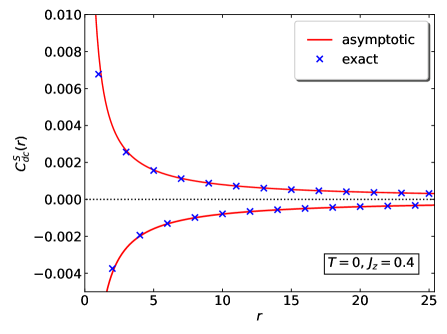
Figure 12: Spin correlation function as a function of distance $r$ from the impurity for $J_{z}=4V=0.4$ at temperature $T=0$ in one dimension. The numerical data are compared with the asymptotic expressions (125).

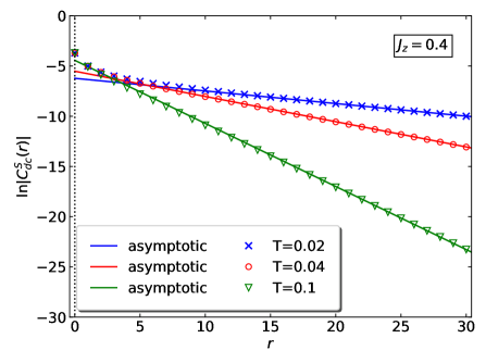
Figure 13: Logarithm of the absolute value of the spin correlation function as a function of distance $r$ from the impurity for $J_{z}=4V=0.4$ at temperatures $T=0.02$, $T=0.04$, $T=0.1$ in one dimension. The numerical data are compared with the analytically determined exponential decay with exponent $(\xi_{2})^{-1}=2\pi T$, see eq. (127).

In Fig. 13 we show the logarithm of the absolute value of the spin correlation function as a function of distance for $J_{z}=4V=0.4$ for various small temperatures. It is seen that the correlation function decays to zero exponentially. The correlation length agrees with the analytically determined value $(\xi_{2})^{-1}=2\pi T$ from eq. (127), as derived in Sect. 4.2.3.

4.2.2 Asymptotics at zero temperature

The pole contribution to the spin correlation function decays exponentially for all temperatures, as has to be expected for bound and anti-bound states that are localized around the impurity. Therefore, the long-range asymptotic is governed by the Friedel oscillations of the band contribution. We focus on the limit of small interactions, $V=J_{z}/4\ll 1$.

For the band contribution to the correlation function we consider at $T=0$

$$C_{dc}^{S,{\rm b}}(r,T=0)=\frac{V}{2\pi}c^{S}(r,V)$$ (121)

with

$$c^{S}(r,V) = (-1)^{r}\int_{-\pi/2}^{0}{\rm d}p\frac{\sin(2pr)\cos(p)}{V^{2}+\cos^{2}(p)}$$

$$= \int_{0}^{\pi/2}{\rm d}u\frac{\sin(2ur)}{\sin(u)}\left(1-\frac{V^{2}}{\sin^{2}(u)+V^{2}}\right)\;.$$

The first term in the brackets can be integrated analytically using Mathematica [19],

$$c_{1}^{S}(r,V) = \frac{1}{4}\biggl{[}\psi\left(\frac{1}{4}+\frac{r}{2}\right)-\psi\left(\frac{1}{4}-\frac{r}{2}\right)$$ (123)

$$\hphantom{\frac{1}{4}\Bigl{[}}-\psi\left(\frac{3}{4}+\frac{r}{2}\right)+\psi\left(\frac{3}{4}-\frac{r}{2}\right)\biggr{]}$$

$$\approx \frac{\pi}{2}-(-1)^{r}\frac{1}{2r}\quad\hbox{for}\;r\gg 1\;,$$

where $\psi(x)=\Gamma^{\prime}(x)/\Gamma(x)$ is the digamma function.

The integrand in the second term of eq. (4.2.2) is of the order $V^{2}$ when $\sin(u)$ is of order unity. Therefore, only small arguments are of interest,

$$c_{2}^{S}(r,V) \approx -\int_{0}^{\gamma V}{\rm d}u\frac{\sin(2ru)}{u}\frac{V^{2}}{u^{2}+V^{2}}$$ (124)

$$\approx -\int_{0}^{\infty}{\rm d}x\frac{(2rV)^{2}}{x^{2}+(2rV)^{2}}\frac{\sin(x)}{x}$$

$$= -\frac{\pi}{2}\left(1-e^{-2rV}\right)$$

$$\approx -\frac{\pi}{2}\quad\hbox{for}\;r\gg 1$$

with $\gamma$ smaller than one but of the order unity so that $2r\gamma V\gg 1$ for $r\gg 1$. The integral was evaluated using Mathematica [19].

Summing the two terms from eq. (123) and (124) gives the long-range asymptotics of the spin correlation function at zero temperature for small interaction strengths, $V\ll 1$,

$$C_{dc}^{S,{\rm b}}(r\gg 1,T=0)=-(-1)^{r}\frac{V}{4\pi r}\;.$$ (125)

The correlation function decays to zero algebraically, and displays Friedel oscillations [2] that are commensurate with the lattice at half band-filling.

4.2.3 Asymptotics at finite temperature

At finite temperature and small interactions $V=J_{z}/4\ll 1$, the correlation function decays to zero exponentially as a function of distance $r$ from the impurity,

$$C_{dc}^{S}(r\gg 1,T>0)\sim(-1)^{r}e^{-r/\xi_{2}(T)}$$ (126)

with

$$\xi_{2}(T)=\frac{1}{2\pi T}\;.$$ (127)

A detailed derivation is given in Appendix B.3. Note that the same correlation length was obtained earlier for the non-interacting single-impurity Anderson model [11].

4.3 Screening cloud in one dimension

Lastly, we discuss the screening cloud. We analytically derive the long-range asymptotics of the unscreened spin.

4.3.1 Analytic expressions

We have $C_{dd}^{S}=1/4$ from eq. (32) and $C_{dc}(0)=C_{dc}^{\rm p}(0)$. After summing the spin correlation function from $|r|=1$ up to $|r|=R$ we find for the unscreened spin at distance $R\geq 1$

$${\cal S}^{\rm 1d}(R,T,V) = \frac{1}{4}\left(1-\frac{V}{\sqrt{1+V^{2}}}\tanh\biggl{[}\frac{\sqrt{1+V^{2}}}{2T}\biggr{]}\right)$$ (128)

$$+s_{R}^{\rm p}(T,V)+s_{R}^{\rm b}(T,V)$$

with ($K=V+\sqrt{1+V^{2}},1-K^{2}=-2VK$)

$$s_{R}^{\rm p}(T,V)=-\tanh\left(\frac{\sqrt{1+V^{2}}}{2T}\right)\frac{\left(1-K^{-2R}\right)}{4K\sqrt{1+V^{2}}}\;,$$ (129)

and

$$s_{R}^{\rm b}(T,V) = \frac{V}{2\pi}\int_{-\pi/2}^{\pi/2}{\rm d}pf(\sin(p),T)\frac{1}{V^{2}+\cos^{2}(p)}$$

$$\hphantom{\frac{V}{2\pi}}\times\left((-1)^{R}\sin[(2R+1)p]-\sin(p)\right)$$

$$= -\frac{V}{2\pi}\int_{0}^{\pi/2}{\rm d}p\tanh\left[\frac{\sin(p)}{2T}\right]\frac{1}{V^{2}+\cos^{2}(p)}$$

$$\hphantom{\frac{V}{2\pi}}\times\left((-1)^{R}\sin[(2R+1)p]-\sin(p)\right)\;.$$

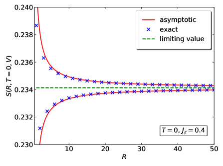
Figure 14: Unscreened spin as a function of distance $R$ from the impurity for $J_{z}=4V=0.4$ at temperature $T=0$ in one dimension. The numerical data are compared with the limiting value (131) and the asymptotic behavior (132) for small couplings.

In Fig. 14 we show the unscreened spin as a function of distance in the ground state for $J_{z}=4V=0.4$. Even at zero temperature, the impurity spin is not completely screened at infinite distance from the impurity but reaches the limiting value given in eq. (131), as derived in Sect. 4.3.2. The unscreened spin displays Friedel oscillations around its limiting value that decay algebraically to zero, see eq. (132).

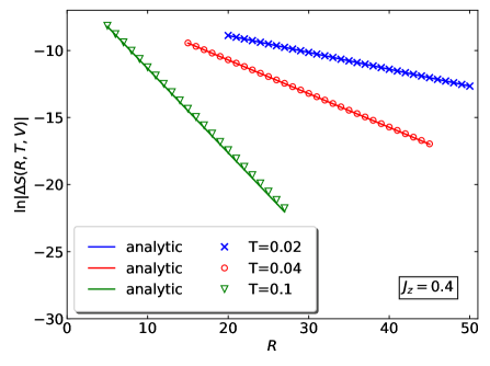
Figure 15: Logarithm of the decaying part of the unscreened spin, $\Delta{\cal S}(R,T,V)=|{\cal S}^{\rm 1d}(R,T,V)-S_{\infty}^{\rm 1d}(T,V)|$, as a function of distance $R$ from the impurity for $J_{z}=4V=0.4$ at temperatures $T=0.02$, $T=0.04$, $T=0.1$ in one dimension. The numerical data are compared with the analytically determined exponential decay with exponent $(\xi_{2})^{-1}=2\pi T$, see eq. (136).

In Fig. 15 we show the decaying part of the unscreened spin, $\Delta{\cal S}(R,T,V)=|{\cal S}^{\rm 1d}(R,T,V)-S_{\infty}^{\rm 1d}(T,V)|$, as a function of distance for $J_{z}=4V=0.4$ for various small temperatures. It is seen that the correlation function decays to zero exponentially. The correlation length agrees with the analytically determined value $(\xi_{2})^{-1}=2\pi T$ from eq. (136), as derived in Sect. 4.3.3.

4.3.2 Asymptotics at zero temperature

First, we determine the unscreened spin in the ground state for $R\to\infty$. As shown in Appendix A.5, the Friedel sum rule [2] gives

$${\cal S}_{\infty}^{\rm 1d}(V) = \lim_{R\to\infty}{\cal S}^{\rm 1d}(R,T=0,V)$$ (131)

$$= \frac{1}{4}+\frac{1}{2}\Delta N_{0}^{\rm 1d}(T=0,V)$$

$$= \frac{1}{4}-\frac{1}{2\pi}\arctan(V)$$

because $\Delta N_{0}(T,-V)=-\Delta N_{0}(T,V)$, see eq. (209) in appendix A.5.3. For all finite interactions, the impurity spin is not completely screened, ${\cal S}_{\infty}(T,V)>0$, even at zero temperature. In fact, for small interactions, $V\ll 1$, we have ${\cal S}_{\infty}^{\rm 1d}(V\ll 1)\approx 1/4-V/(2\pi)$, i.e., the screening is very small, of the order $V$.

Next, we use eq. (125) to determine the approach of the unscreened spin to its limiting value for small $V$,

$${\cal S}^{\rm 1d}(R,T=0,V)-{\cal S}_{\infty}^{\rm 1d}(V)\approx-\frac{(-1)^{R}}{4\pi R}V+{\cal O}\left(V^{3}/R\right)\;.$$ (132)

The Friedel oscillations seen in the correlation function also show up in the unscreened spin.

4.3.3 Asymptotics at small temperatures

As discussed in Appendix A.5, the Friedel sum rule is slightly modified at finite temperatures ($\beta=1/T$),

$${\cal S}_{\infty}^{\rm 1d}(T,V) = \lim_{R\to\infty}{\cal S}^{\rm 1d}(R,T,V)$$ (133)

$$= \frac{1}{4}-\frac{\left[\exp\left(\beta\sqrt{1+V^{2}}\right)-\exp(\beta)\right]\!/2}{\left(1+\exp\left(\beta\sqrt{1+V^{2}}\right)\right)\left(1+\exp(\beta)\right)}$$

$$-\int_{-\beta/2}^{\beta/2}{\rm d}x\arctan\left[\frac{V}{\sqrt{1-(2x/\beta)^{2}}}\right]$$

$$\hphantom{-\int_{-\beta/2}^{\beta/2}{\rm d}x}\times\frac{1}{4\pi\cosh^{2}(x)}\;.$$

At low temperatures, we find

$${\cal S}_{\infty}^{\rm 1d}(T\ll 1,V)\approx\frac{1}{4}-\frac{1}{2\pi}\arctan(V)-\frac{\pi}{12}\frac{V}{1+V^{2}}T^{2}\;,$$ (134)

with corrections of the order $VT^{4}$. In one dimension, the density of states increases around the Fermi energy. Therefore, at finite temperatures, more electrons are available to screen the impurity spin so that the screening becomes a little bit more effective for small but finite temperatures than in the ground state. Note, however, that the corrections are small, of the order $VT^{2}$ for small $V$ and $T$.

At finite temperature and small interactions $V=J_{z}/4\ll 1$, as seen from Fig. 15, the amount of the unscreened spin decays exponentially to its limiting value $S_{\infty}(T,V)$ as a function of distance $r$ from the impurity,

$${\cal S}(R\gg\xi_{2},T,V)={\cal S}_{\infty}(T,V)+\tilde{s}(T,V)(-1)^{R}e^{-R/\xi_{2}(T)}$$ (135)

with an unspecified proportionality constant $\tilde{s}(T,V)$ and the correlation length

$$\xi_{2}(T)=\frac{1}{2\pi T}$$ (136)

in one dimension. A detailed derivation is given in Appendix B.2.

5 Conclusions

In this work, we calculated and discussed the thermodynamics and spin correlations in the exactly solvable Ising-Kondo model. In this problem, the impurity spin orientation is dynamically conserved so that the partition function and thermal expectation values can be expressed in terms of the single-particle density of states of spinless fermions with a local scattering potential.

As examples, we studied in detail the case of nearest-neighbor hopping on a chain and on a Bethe lattice with infinite coordination number at half band-filling. The latter condition considerably simplifies the analysis because it fixes the chemical potential to zero for all temperatures and interaction strengths. We gave explicit equations for the free energy, several thermodynamic potentials such as the internal energy, entropy, and magnetization, and response functions such as the specific heat and magnetic susceptibilities.

The Ising-Kondo model provides an instructive example for static screening. At zero external magnetic field, the impurity scattering is attractive for one spin species of the host electrons and repulsive for the other. For an antiferromagnetic Ising-Kondo coupling, host electrons with spin opposite to the impurity accumulate near the impurity site and partially screen the localized spin.

Since there is no dynamic coupling of the two impurity spin orientations in the Ising-Kondo model, the ground state remains doubly degenerate. This is seen in the impurity-induced entropy that remains $S^{\rm spin}(T=0)=\ln(2)$ at zero temperature. Due to the thermally activated screening, the impurity-induced entropy is reduced from its limiting value for all temperatures, as seen in Fig. 3. As a consequence, the impurity contribution to the specific heat is negative at low temperatures, see Fig. 4.

The static screening also shows up for small external magnetic fields $B$. At low temperatures, $T\lesssim B$, the thermodynamics of the Ising-Kondo model becomes identical to that of a free spin in an effective magnetic field, see Figs. 8 and 9, e.g., the impurity-induced zero-field susceptibility obeys a Curie law. The effective field $B^{\rm eff}(B,J_{z})$ is smaller than the external field $B$ due to the antiferromagnetic screening by the host electrons. Alternatively, one may argue that the host electrons reduce the size of the local spin to $S^{\rm eff}<1/2$. This effective spin remains finite as long as the Ising-Kondo interaction does not diverge. In our work, we provide explicit results for the effective field as a function of temperature $T$, external magnetic field $B$, and Ising-Kondo interaction $J_{z}$.

The incomplete static screening is also seen in the spin correlation function. In the ground state, the spin correlation function displays an algebraic decay to zero with commensurate Friedel oscillations, see Fig. 12. At finite temperatures and in one dimension, the spin correlations decay exponentially with correlation length $\xi(T)=1/(2\pi T)$ for weak interactions, see Fig. 13. For $J_{z}\ll 1$, the correlation length is independent of the Ising-Kondo interaction and identical to that for the non-interacting single-impurity Anderson model [11]. The amount of unscreened spin remains finite at zero temperature even at infinite distance from the impurity, see Fig. 14.

The extensive analysis in our work provides tangible results for a non-trivial many-particle problem. The explicit formulae may be used as benchmark tests for sophisticated numerical methods that can be applied to general many-body problems such as the (anisotropic) Kondo model; recall that the Ising-Kondo model is the limiting case of the anisotropic Kondo model where the spin-flip terms are completely suppressed. Thus, the Ising-Kondo model may also serve as a starting point for the analysis of the Kondo model for large anisotropy. However, when pursuing the goal of an analytical approach to the Kondo model, a systematic treatment of spin-flip excitations for the description of dynamical screening in the Kondo model continues to pose an intricate many-particle problem.

Z.M.M. Mahmoud thanks the Fachbereich Physik at the Philipps Universität Marburg for its hospitality during his research stay. The authors extend their appreciation to the Deanship of Scientific Research at King Khalid University for funding this work through research groups program under grant number G.R.P-36-41.

Appendix A Spinless fermions

We treat spinless fermions that interact with a scattering potential at the lattice origin

$$\hat{H}_{\rm ps} = \sum_{i,j}t_{i,j}\hat{c}_{i}^{+}\hat{c}_{j}^{\vphantom{+}}+V\hat{c}_{0}^{+}\hat{c}_{0}^{\vphantom{+}}$$ (137)

$$= \sum_{k}\epsilon(k)\hat{a}_{k}^{+}\hat{a}_{k}^{\vphantom{+}}+\frac{V}{L}\sum_{k,p}\hat{a}_{k}^{+}\hat{a}_{p}^{\vphantom{+}}$$

for a $L$-site system with periodic boundary conditions. This textbook problem is addressed, e.g., in Ref. [20] for a quadratic dispersion relation.

In the main text, we encounter the case where an external field of strength $B$ couples to each fermion mode,

$$\hat{H}_{\rm sf}(B)=\hat{H}_{\rm ps}-\hat{H}_{\rm ext}\;,\quad\hat{H}_{\rm ext}=B\sum_{k}\hat{a}_{k}^{+}\hat{a}_{k}^{\vphantom{+}}\;.$$ (138)

The external field acts like an external chemical potential because it couples to the operator for the particle number

$$\hat{N}=\sum_{k}\hat{a}_{k}^{+}\hat{a}_{k}^{\vphantom{+}}\;.$$ (139)

Therefore, we first consider $\hat{H}_{\rm ps}$ alone, and later absorb $B$ in the chemical potential when we focus on $\hat{H}_{\rm sf}$.

A.1 Calculation of the Green function

We need to calculate the retarded Green function

$$G_{k,p}^{\rm ret}(t)=(-{\rm i})\theta_{\rm H}(t)\langle\left[\hat{a}_{k}^{\vphantom{+}}(t),\hat{a}_{p}^{+}\right]_{+}\rangle\;,$$ (140)

where $\hat{A}(t)=\exp({\rm i}\hat{H}_{\rm ps}t)\hat{A}\exp(-{\rm i}\hat{H}_{\rm ps}t)$ is the Heisenberg operator assigned to the Schrödinger operator $\hat{A}$, and $\theta_{\rm H}(x)$ is the Heaviside step function. The discussion closely follows Ref. [21].

A.1.1 Equation-of-motion method

The derivative of the retarded Green function obeys

$${\rm i}\dot{G}_{k,p}^{\rm ret}(t)=\delta_{k,p}\delta(t)+\epsilon(k)G_{k,p}^{\rm ret}(t)+\frac{V}{L}\sum_{p^{\prime}}G_{p^{\prime},p}^{\rm ret}(t)\;.$$ (141)

A Fourier transformation leads to the result ($\eta=0^{+}$)

$$\tilde{G}_{k,p}^{\rm ret}(\omega)=\frac{\delta_{k,p}+VH_{p}(\omega)}{\omega-\epsilon(k)+{\rm i}\eta}$$ (142)

with the abbreviation

$$H_{p}(\omega)=\frac{1}{L}\sum_{p^{\prime}}\tilde{G}_{p^{\prime},p}^{\rm ret}(\omega)\;.$$ (143)

We insert eq. (142) into eq. (143) to find

$$H_{p}(\omega) = \frac{1}{L}\sum_{p^{\prime}}\frac{\delta_{p^{\prime},p}+VH_{p}(\omega)}{\omega-\epsilon(p^{\prime})+{\rm i}\eta}$$

$$= \frac{1}{L}\frac{1}{\omega-\epsilon(p)+{\rm i}\eta}+Vg_{0}(\omega)H_{p}(\omega)\;,$$

$$H_{p}(\omega) = \frac{1}{L}\frac{1}{1-Vg_{0}(\omega)}\frac{1}{\omega-\epsilon(p)+{\rm i}\eta}\;,$$ (144)

where

$$g_{0}(\omega)=\frac{1}{L}\sum_{p}\frac{1}{\omega-\epsilon(p)+{\rm i}\eta}=\Lambda_{0}(\omega)-{\rm i}\pi\rho_{0}(\omega)$$ (145)

is the local Green function of the non-interacting host fermions; eqs. (8) and (9) [eqs. (10) and (11)] give explicit expressions for nearest-neighbor transfers on a chain [on a Bethe lattice with infinite coordination number].

Then, the solution of eq. (142) can be cast into the form

$$\tilde{G}_{k,p}^{\rm ret}(\omega) = \tilde{G}_{k,p}^{\rm ret,h}(\omega)+\tilde{G}_{k,p}^{\rm ret,i}(\omega)\;,$$

$$\tilde{G}_{k,p}^{\rm ret,h}(\omega) = \frac{\delta_{k,p}}{\omega-\epsilon(k)+{\rm i}\eta}\;,$$

$$\tilde{G}_{k,p}^{\rm ret,i}(\omega) = \frac{V/L}{1-Vg_{0}(\omega)}\frac{1}{\omega-\epsilon(k)+{\rm i}\eta}\frac{1}{\omega-\epsilon(p)+{\rm i}\eta}\,.$$

The host-electron part $\tilde{G}_{k,p}^{\rm ret,h}(\omega)$ provides a bulk contribution that is independent of $V$. Only the impurity-induced part $\tilde{G}_{k,p}^{\rm ret,i}(\omega)$ of order unity is relevant for our further considerations.

A.1.2 Density of states

The impurity-induced contribution to the single-particle density of states is given by

$$D_{0}(\omega) = -\frac{1}{\pi}{\rm Im}\left(\sum_{k}\tilde{G}_{k,k}^{\rm ret}(\omega)\right)-L\rho_{0}(\omega)$$ (147)

$$= -{\rm Im}\biggl{[}\frac{1}{\pi L}\sum_{k}\frac{V}{1-Vg_{0}(\omega)}\Bigl{(}\frac{1}{\omega-\epsilon(k)+{\rm i}\eta}\Bigr{)}^{2}\biggr{]}$$

$$= -\frac{1}{\pi}\frac{\partial}{\partial\omega}{\rm Im}\left[\ln\left(1-Vg_{0}(\omega)\right)\right].$$

For general $g_{0}(\omega)$ we note the useful relation

$$D_{0}(-\omega,-V)=D_{0}(\omega,V)\;,$$ (148)

where we made explicit the $V$-dependence of the impurity-induced contribution to the density of states. Moreover,

$$\int_{-\infty}^{\infty}{\rm d}\omega D_{0}(\omega,V)=0$$ (149)

where we use eq. (147) and the fact $g_{0}(|\omega|\to\infty)=0$.

One-dimensional host-electron density of states

Let $|\omega|>1$. We obtain the (anti-)bound state from

$$1-V\Lambda_{0}(\omega_{\rm b,ab})=0\;.$$ (150)

For the one-dimensional case we thus find

$$\omega_{\rm b,ab}=\pm\sqrt{1+V^{2}}\;.$$ (151)

There is a bound state at $\omega_{\rm b}=-\sqrt{1+V^{2}}$ for $V<0$ and an anti-bound state at $\omega_{\rm ab}=\sqrt{1+V^{2}}$ for $V>0$. To calculate the contribution to the density of states from the bound states outside the band where we have $\rho_{0}(\omega)=\eta\equiv 0^{+}$, we expand

$${\rm R}(\omega)\equiv 1-V\Lambda_{0}(\omega)\approx{\rm R}^{\prime}(\omega_{0})(\omega-\omega_{0})$$ (152)

in the vicinity of $\omega_{0}\equiv\omega_{\rm b,ab}$. Then,

$$D_{0}^{\rm b,ab}(\omega) = -\frac{1}{\pi}\frac{\partial}{\partial\omega}\left[\cot^{-1}\left(\frac{{\rm R}^{\prime}(\omega_{0})(\omega-\omega_{0})}{\pi V\eta}\right)\right]$$ (153)

$$= \frac{1}{\pi}\frac{\tilde{\eta}}{\tilde{\eta}^{2}+(\omega-\omega_{0})^{2}}$$

$$= \delta(\omega-\omega_{0})$$

with $\tilde{\eta}=\pi V\eta/{\rm R}^{\prime}(\omega_{0})\to 0^{+}$. Thus, the bound and anti-bound states contribute

$$D_{0}^{\rm b,ab}(\omega)=\delta(\omega-\omega_{\rm b})\theta_{\rm H}(-V)+\delta(\omega-\omega_{\rm ab})\theta_{\rm H}(V)$$ (154)

to the impurity part of the density of states.

For the band contribution we consider the region that includes the band edges, $|\omega|\leq 1^{+}$. In general, we obtain

$$D_{0}^{\rm band}(\omega) = -\frac{1}{\pi}{\rm sgn}(V)\frac{\partial}{\partial\omega}\mathop{\rm Cot}\nolimits^{-1}\left[\varphi(\omega)\right]\;,$$

$$\varphi(\omega) = \frac{1-V\Lambda_{0}(\omega)}{\pi|V|\rho_{0}(\omega)}\;,$$ (155)

where $\mathop{\rm Cot}^{-1}(x)=\pi\theta_{\rm H}(-x)+\cot^{-1}(x)$ is continuous and differentiable across $x=0$, and ${\rm sgn}(x)=x/|x|$ is the sign function.

In one dimension and for $V>0$, the phase $\varphi(\omega)$ jumps by $\pi/2$ when going from $\omega=(-1)^{-}$ to $\omega=(-1)^{+}$. The same jump appears at $\omega=1$. For $V<0$, we obtain the same discontinuities. Inside the band we have instead $\Lambda_{0}(|\omega|<1)=0$ so that we find altogether ($\omega_{\rm p}(V)\equiv\omega_{p}=\sqrt{1+V^{2}}$)

$$D_{0}^{\rm 1d}(\omega) = \delta(\omega+\omega_{\rm p})\theta_{\rm H}(-V)+\delta(\omega-\omega_{\rm p})\theta_{\rm H}(V)$$

$$-\frac{1}{2}\delta(\omega+1)-\frac{1}{2}\delta(\omega-1)$$

$$-\theta_{\rm H}(1^{-}-|\omega|)\frac{1}{\pi}\frac{\partial}{\partial\omega}\arctan\left[\frac{V}{\sqrt{1-\omega^{2}}}\right]\;.$$

Semi-elliptic host-electron density of states

For the semi-elliptic density of states, see eqs. (10) and (11), there are no bound states for $V<1/2$ [10] and no singularities at the band edges. Therefore, the semi-elliptic density of states displays only a band contribution,

$$D_{0}^{\rm se}(\omega)=-\theta_{\rm H}(1-|\omega|)\frac{1}{\pi}\frac{\partial}{\partial\omega}\arctan\biggl{[}\frac{2V\sqrt{1-\omega^{2}}}{1-2\omega V}\biggr{]}\;.$$ (157)

A.2 Ground-state energy

When we calculate the ground-state energy, we need to know the Fermi energy. At half band-filling, the interaction-induced changes in the Fermi energy vanish in the thermodynamic limit and thus are irrelevant for the calculation of the interaction-induced change in the ground-state energy.

A.2.1 Fermi energy

The impurity Hamiltonian (137) is not particle-hole symmetric. Therefore, the Fermi energy $\epsilon_{\rm F}(V)$ depends on $V$. Since the scattering only appears at a single site, we have

$$\epsilon_{\rm F}(V)=\epsilon_{\rm F}^{(0)}+\frac{\epsilon_{\rm F}^{(1)}(V)}{L}$$ (158)

to leading order in $1/L$. Here, $\epsilon_{\rm F}^{(0)}$ is determined from the particle number,

$$N=L\int_{-\infty}^{\epsilon_{\rm F}^{(0)}}{\rm d}\omega\rho_{0}(\omega)\;.$$ (159)

At half band-filling, $N=L/2$, and for a symmetric density of states, $\rho_{0}(-\omega)=\rho_{0}(\omega)$, it is readily shown that the bulk Fermi energy is zero, $\epsilon_{\rm F}^{(0)}=0$.

We can calculate $\epsilon_{\rm F}^{(1)}(V)$ from

$$0=L\int_{\epsilon_{\rm F}^{(0)}}^{\epsilon_{\rm F}^{(0)}+\epsilon_{\rm F}^{(1)}(V)/L}{\rm d}\omega\rho_{0}(\omega)+\int_{-\infty}^{\epsilon_{\rm F}^{(0)}}{\rm d}\omega D_{0}(\omega,V)\;,$$ (160)

so that

$$\epsilon_{\rm F}^{(1)}(V)=-\frac{1}{\rho_{0}(\epsilon_{\rm F}^{(0)})}\int_{-\infty}^{\epsilon_{\rm F}^{(0)}}{\rm d}\omega D_{0}(\omega,V)$$ (161)

in the thermodynamic limit.

At half band-filling, we do not need the correction to calculate the ground-state energy because $\epsilon_{\rm F}^{(0)}=0$ and the bulk contribution to the energy is

$$E_{0}^{\rm bulk}(V) = L\int_{-\infty}^{0}{\rm d}\omega\omega\rho_{0}(\omega)+L\int_{0}^{\epsilon_{\rm F}^{(1)}/L}{\rm d}\omega\omega\rho_{0}(\omega)$$ (162)

$$= E_{0}^{\rm bulk}(V=0)+L\rho_{0}(0)\frac{1}{2}\left(\frac{\epsilon_{\rm F}^{(1)}}{L}\right)^{2}$$

$$= E_{0}^{\rm bulk}(V=0)+{\cal O}(1/L)\;.$$

Thus, we can calculate the scattering contribution to the ground-state energy from the single-particle density of states as

$$e_{0}(V)=E_{0}(V)-E_{0}^{\rm bulk}(V=0)=\int_{-\infty}^{0}{\rm d}\omega\omega D_{0}(\omega,V)\;.$$ (163)

In Sect. A.1.2 we provide explicit expressions for the impurity-induced single-particle density of states $D_{0}(\omega,V)$ for nearest-neighbor electron transfer on a chain and on a Bethe lattice with infinite coordination number, see Sect. 2.1.1.

A.2.2 One-dimensional density of states

There is no bound state for $V>0$ and the ground-state energy can be calculated from the band contribution alone,

$$e_{0}^{\rm 1d}(V>0) = \frac{1}{2}-\frac{1}{\pi}\biggl{[}\omega\arctan\left(\pi V\rho_{0}(\omega)\right)\biggr{]}_{-1^{+}}^{0}$$ (164)

$$+\frac{1}{\pi}\int_{-1}^{0}{\rm d}\omega\arctan\left[\pi V\rho_{0}(\omega)\right]$$

$$= \frac{1}{\pi}\int_{-1}^{0}{\rm d}\omega\arctan\left[\pi V\rho_{0}(\omega)\right]$$

$$= \frac{1}{2}\left(1+V-\sqrt{1+V^{2}}\right)\;.$$

For the last step we rely on Mathematica [19].

For attractive interactions, $V<0$, we can investigate the particle-hole transformed Hamiltonian,

$$\tau_{\rm ph}^{+}\hat{H}_{\rm ps}(V)\hat{\tau}_{\rm ph}=\hat{H}_{\rm ps}(-V)+V\;.$$ (165)

At half filling, this implies for the scattering contribution to the ground-state energy

$$e_{0}(V)=V+e_{0}(-V)\;.$$ (166)

Thus, we find $(V<0)$

$$e_{0}^{\rm 1d}(V) = V+\frac{1}{2}\left(1-V-\sqrt{1+V^{2}}\right)$$ (167)

$$= \frac{1}{2}\left(1+V-\sqrt{1+V^{2}}\right)\;.$$

Eq. (167) is formally identical to eq. (164).

Alternatively, we can calculate $e_{0}(V)$ for $V<0$ from the density of states. We include the bound state and find

$$e_{0}^{\rm 1d}(V<0) = -\sqrt{1+V^{2}}+\frac{1}{2}$$ (168)

$$+\frac{1}{\pi}\biggl{[}\omega\arctan\left(\pi|V|\rho_{0}(\omega)\right)\biggr{]}_{-1^{+}}^{0}$$

$$-\frac{1}{\pi}\int_{-1^{+}}^{0}{\rm d}\omega\arctan\left[\pi|V|\rho_{0}(\omega)\right]$$

$$= \frac{1}{2}\left(1+V-\sqrt{1+V^{2}}\right)\;,$$

which is identical to eq. (167), and

$$e_{0}^{\rm 1d}(V)=\frac{1}{2}\left(1+V-\sqrt{1+V^{2}}\right)$$ (169)

holds for all $V$.

A.2.3 Semi-elliptic density of states

For the density of states in eq. (10) and $0<V<1/2$ there are no (anti-)bound states [10]. Eq. (163) gives

$$e_{0}^{\rm se}(V>0) = -\frac{1}{\pi}\int_{-1}^{0}{\rm d}\omega\,\omega\frac{\partial}{\partial\omega}\arctan\left[\frac{2V\sqrt{1-\omega^{2}}}{1-2V\omega}\right]$$

$$= \frac{1}{\pi}\int_{-1}^{0}{\rm d}\omega\arctan\left[\frac{2V\sqrt{1-\omega^{2}}}{1-2V\omega}\right]$$

$$= \frac{1}{2\pi}+\frac{V}{2}-\frac{1+4V^{2}}{8\pi V}\arctan\left[\frac{4V}{1-4V^{2}}\right]$$

after a partial integration. In the last step, we used Mathematica [19] to carry out the integration. For $-1/2<V<0$ we verified that $e_{0}^{\rm se}(-|V|)$ obeys eq. (166).

A.3 Free energy (potential scattering)

We consider the case of potential scattering only. Before we can calculate the free energy, we must determine the chemical potential $\mu(N,T,V)$.

A.3.1 Chemical potential

For finite temperatures $T$, eq. (158) generalizes to

$$\mu(N,T,V)=\mu^{(0)}(N,T)+\frac{\mu^{(1)}(N,T,V)}{L}$$ (171)

to leading order in $1/L$. By definition, $\mu^{(0)}(N,T)$ is the chemical potential for non-interacting spinless fermions at temperature $T$ with average particle number $N$,

$$N=L\int_{-\infty}^{\infty}{\rm d}\omega\frac{\rho_{0}(\omega)}{1+\exp[\beta(\omega-\mu^{(0)}(N,T)]}\;,$$ (172)

where $\beta=1/T$. When we consider the particle number $N$ as a function of $\mu^{(0)}(T)$, we can use particle-hole symmetry, $\rho_{0}(\omega)=\rho_{0}(-\omega)$, to write

$$N(\mu^{(0)}(T)) = L\int_{-\infty}^{\infty}{\rm d}\omega\frac{\rho_{0}(\omega)}{1+\exp[\beta(-\omega-\mu^{(0)}(T)]}$$ (173)

$$= L\int_{-\infty}^{\infty}{\rm d}\omega\frac{\rho_{0}(\omega)\exp[\beta(\omega+\mu^{(0)}(T)]}{1+\exp[\beta(\omega+\mu^{(0)}(T)]}$$

$$= L-N(-\mu^{(0)}(T))\;.$$

which implies

$$\mu^{(0)}(L-N,T)=-\mu^{(0)}(N,T)\;,$$ (174)

i.e., when $\mu^{(0)}(T)$ fixes the average particle number to $N$, the chemical potential $-\mu^{(0)}(T)$ leads to the average particle number to $L-N$. Thus, for half band-filling, a zero chemical potential

$$\mu^{(0)}(T)=0\;,$$ (175)

implies half band-filling, $N=L/2$, for all temperatures.

In the thermodynamic limit, we can calculate the correction $\mu^{(1)}(N,T,V)$ in eq. (171) from

$$0 = -L\int_{-\infty}^{\infty}{\rm d}\omega\frac{\rho_{0}(\omega+\mu^{(0)}(N,T))}{1+\exp(\beta\omega)}$$ (176)

$$+L\int_{-\infty}^{\infty}{\rm d}\omega\frac{\rho_{0}(\omega+\mu^{(0)}(N,T))}{1+\exp[\beta(\omega-\mu^{(1)}(N,T,V)/L)]}$$

$$+\int_{-\infty}^{\infty}{\rm d}\omega\frac{D_{0}(\omega+\mu^{(0)}(N,T))}{1+\exp(\beta\omega)}\;,$$

where we used $D(\omega)=L\rho_{0}(\omega)+D_{0}(\omega)$ so that

$$\mu^{(1)}(N,T,V) = -\frac{A_{1}(N,T,V)}{A_{2}(N,T)}\;,$$

$$A_{1}(N,T,V) = \int_{-\infty}^{\infty}{\rm d}\omega\frac{D_{0}(\omega+\mu^{(0)}(N,T),V)}{1+\exp(\beta\omega)}\;,$$

$$A_{2}(N,T) = \int_{-\infty}^{\infty}{\rm d}\omega\frac{\rho_{0}(\omega+\mu^{(0)}(N,T))\beta\exp(\beta\omega)}{[1+\exp(\beta\omega)]^{2}}$$

in the thermodynamic limit. Note that, for $T\to 0$, we recover $\mu^{(1)}(T=0,N,V)=\epsilon_{\rm F}^{(1)}(V)$ from eq. (161).

With eq. (148) it is readily shown that

$$A_{1}(L-N,T,-V) = \int_{-\infty}^{\infty}\!{\rm d}\omega\frac{D_{0}(\omega+\mu^{(0)}(N,T),V)}{1+\exp(-\beta\omega)}$$ (178)

$$= \int_{-\infty}^{\infty}\!{\rm d}\omega D_{0}(\omega+\mu^{(0)}(N,T,V))$$

$$-\int_{-\infty}^{\infty}\!{\rm d}\omega\frac{D_{0}(\omega+\mu^{(0)}(N,T),V)}{1+\exp(\beta\omega)}$$

$$= -A_{1}(N,T,V)\;,$$

where we used eqs. (149) and (174). Likewise we find

$$A_{2}(L-N,T)=A_{2}(N,T)\;.$$ (179)

Thus,

$$\mu^{(1)}(L-N,T,-V)=-\mu^{(1)}(N,T,V)\;.$$ (180)

A.3.2 Free energy

For non-interacting fermions with single-particle density of states $D(\omega)$, the free energy can be written as [16, 17]

$$F=-T\int_{-\infty}^{\infty}{\rm d}\omega\ln\left(1+\exp[-\beta(\omega-\mu]\right)D(\omega)\;,$$ (181)

where $F\equiv F(N,T)$, $\mu\equiv\mu(N,T)$ for notational simplicity. For the spinless fermion model in eq. (137) we use $D(\omega,V)=L\rho_{0}(\omega)+D_{0}(\omega,V)$ to write ($\mu^{(0)}\equiv\mu^{(0)}(N,T)$, $\mu^{(1)}\equiv\mu^{(1)}(N,T,V)$)

$$F_{\rm ps} = -TL\int_{-\infty}^{\infty}\!{\rm d}\omega\ln\Big{[}1+e^{-\beta(\omega-\mu^{(1)}/L)}\Bigr{]}\rho_{0}(\omega+\mu^{(0)})$$

$$-T\int_{-\infty}^{\infty}{\rm d}\omega\ln\left(1+e^{-\beta\omega}\right)D_{0}(\omega+\mu^{(0)},V)$$

$$= F_{\rm ps}^{(0)}-\mu^{(1)}\int_{-\infty}^{\infty}{\rm d}\omega\frac{\rho_{0}(\omega+\mu^{(0)})}{1+\exp(\beta\omega)}$$

$$-T\int_{-\infty}^{\infty}{\rm d}\omega\ln\left(1+e^{-\beta\omega}\right)D_{0}(\omega+\mu^{(0)},V)\;,$$

where $F_{\rm ps}^{(0)}\equiv F_{\rm ps}(N,T)=F_{\rm ps}(N,T,V=0)$ is the free energy for free spinless fermions,

$$F_{\rm ps}^{(0)}=-T\int_{-\infty}^{\infty}{\rm d}\omega\ln\left(1+\exp[-\beta(\omega-\mu^{(0)}]\right)\rho_{0}(\omega)\;.$$ (183)

Using the definition of $\mu^{(0)}$ in eq. (172), we readily find

$$F_{\rm ps}(N,T,V) = F_{\rm ps}^{(0)}(N,T)-\mu^{(1)}(N,T,V)\frac{N}{L}$$

$$+F_{\rm ps}^{\rm i}(N,T,V)\;,$$

$$F_{\rm ps}^{\rm i}(N,T,V) = -T\int_{-\infty}^{\infty}{\rm d}\omega\ln\left(1+e^{-\beta\omega}\right)$$

$$\hphantom{-T\int_{-\infty}^{\infty}}\times D_{0}(\omega+\mu^{(0)}(N,T),V)\,.$$

A.4 Free energy (external field)

In the following, we consider $\hat{H}_{\rm sf}$, see eq. (138), where the spinless fermions encounter an external field. The external field $B$ can be absorbed in the chemical potential, i.e., we simply have to replace $\mu^{(0)}(T)$ by $\mu^{(0)}(T)+B$ in all formulae of the preceding section A.3.

A.4.1 Half band-filling

We focus on a half-filled system at $B=0$, i.e., we set $\mu^{(0)}(T)=0$. Thus, for finite $B$ we have

$$N\equiv N(B)=L\int_{-\infty}^{\infty}{\rm d}\omega\frac{\rho_{0}(\omega)}{1+\exp[\beta(\omega-B)]}$$ (185)

for the particle number. Note that we choose $B$ small enough to not completely fill or empty the system. Note that

$$N(-B)+N(B)=L$$ (186)

which expresses the half-filling condition at $B=0$.

We proceed analogously to Sect. A.3.1 and find

$$\bar{\mu}^{(1)}(B,T,V) = -\frac{\bar{A}_{1}(B,T,V)}{\bar{A}_{2}(B,T)}\;,$$

$$\bar{A}_{1}(B,T,V) = \int_{-\infty}^{\infty}{\rm d}\omega\frac{D_{0}(\omega+B,V)}{1+\exp(\beta\omega)}\;,$$

$$\bar{A}_{2}(B,T) = \int_{-\infty}^{\infty}{\rm d}\omega\frac{\rho_{0}(\omega+B)\beta\exp(\beta\omega)}{[1+\exp(\beta\omega)]^{2}}\;.$$ (187)

In analogy to eq. (180) we have

$$\bar{\mu}^{(1)}(-B,T,-V)=-\bar{\mu}^{(1)}(B,T,V)$$ (188)

for the impurity-induced correction to the chemical potential at half band-filling in the presence of an external field $B$.

For the free energy of a half-filled system in the presence of an external field we find

$$F_{\rm sf}(B,T,V) = F_{\rm sf}^{(0)}(B,T)-\bar{\mu}^{(1)}(B,T,V)\frac{N(B)}{L}$$

$$+F_{\rm sf}^{\rm i}(B,T,V)\;,$$

$$F_{\rm sf}^{\rm i}(B,T,V) = -T\int_{-\infty}^{\infty}{\rm d}\omega\ln\left(1+e^{-\beta\omega}\right)$$ (189)

$$\hphantom{-T\int_{-\infty}^{\infty}}\times D_{0}(\omega+B,V)$$

with $N(B)$ from eq. (185) and

$$F_{\rm sf}^{(0)}(B,T)=-T\int_{-\infty}^{\infty}{\rm d}\omega\ln\left(1+\exp(-\beta\omega)\right)\rho_{0}(\omega+B)$$ (190)

for non-interacting spinless fermions at half band-filling in an external field.

A.4.2 Incomplete free energy

In the main text, we encounter the incomplete partition function

$$\bar{Z}_{\rm sf}=\mathop{\rm Tr}e^{-\beta\hat{H}_{\rm sf}}$$ (191)

that lacks the chemical potential term $\mu^{(1)}$ in the partition function for spinless fermions at half band-filling in the presence of an external field,

$$Z_{\rm sf}=\mathop{\rm Tr}e^{-\beta(\hat{H}_{\rm sf}-\mu^{(1)}\hat{N}/L)}\;,$$ (192)

where $\hat{N}$ is the particle-number operator, see eq. (139).

We add the chemical potential term in eq. (191),

$$\bar{Z}_{\rm sf}=e^{-\beta\mu^{(1)}N/L}\mathop{\rm Tr}e^{-\beta\left(\hat{H}_{\rm sf}-\mu^{(1)}\hat{N}/L+\mu^{(1)}(\hat{N}-N)/L\right)}\;,$$ (193)

where $N$ is the average particle number from eq. (185). Since particle-number fluctuations are small, we may expand

$$\bar{Z}_{\rm sf} \approx Z_{\rm sf}e^{-\beta\mu^{(1)}N/L}\biggl{(}1-\beta\frac{\mu^{(1)}}{L}\langle\hat{N}-N\rangle_{\rm sf}$$

$$\hphantom{e^{-\beta\mu^{(1)}N/L}Z_{\rm sf}\biggl{(}}+\beta^{2}\frac{[\mu^{(1)}]^{2}}{L^{2}}\langle(\hat{N}-N)^{2}\rangle_{\rm sf}\biggr{)}\;,$$

where

$$\langle\hat{A_{\rm sf}}\rangle_{\rm sf}=\frac{1}{Z_{\rm sf}}\mathop{\rm Tr}\left(e^{-\beta(\hat{H}_{\rm sf}-\mu^{(1)}\hat{N}/L)}\hat{A}_{\rm sf}\right)$$ (195)

is the thermal expectation value of an operator $\hat{A}_{\rm sf}$ for the model of spinless fermions, see eq. (117). By construction, $\langle\hat{N}-N\rangle_{\rm sf}=0$. Moreover,

$$\frac{1}{L^{2}}\langle(\hat{N}-N)^{2}\rangle_{\rm sf}=\frac{{\cal O}(N)}{L^{2}}={\cal O}(1/L)$$ (196)

so that the second-order term and all higher-order terms in the expansion in eq. (LABEL:appeq:Zbaraction2) vanish in the thermodynamic limit. Thus,

$$\bar{F}_{\rm sf}=-T\ln\bar{Z}_{\rm sf}=\mu^{(1)}\frac{N}{L}+F_{\rm sf}\;.$$ (197)

Together with eq. (189) we find

$$\bar{F}_{\rm sf}(B,T,V)=F_{\rm sf}^{(0)}(B,T)+F_{\rm sf}^{\rm i}(B,T,V)\;,$$ (198)

as used in the main text.

Eq. (198) shows that the chemical potential $\mu^{(1)}$ is irrelevant for the calculation of the effective free energy $\bar{F}_{\rm sf}(B,T,V)$. This can readily be understood from the fact that, in the grand canonical ensemble, the particle number is only fixed on average, with fluctuations of the order $1/\sqrt{N}$, see eq. (196). Thus, the small changes in the particle number induced by the interaction on a single site can be ignored from the beginning by putting $\mu^{(1)}/L\equiv 0$.

A.5 Local density

For the calculation of the screening cloud, we need the impurity-induced change in the local density,

$$N_{0}(r,T,V)=\langle\hat{c}_{r}^{+}\hat{c}_{r}^{\vphantom{+}}\rangle_{V}-\langle\hat{c}_{r}^{+}\hat{c}_{r}^{\vphantom{+}}\rangle_{V=0}\;.$$ (199)

After a Fourier transformation and using the retarded single-particle Green function, this single-particle expectation value can be expressed as [16]

$$N_{0}(r,T,V)=\frac{1}{L}\sum_{k,p}e^{{\rm i}(k-p)r}\!\int_{-\infty}^{\infty}{\rm d}\omega f(\omega,T)D_{0}(k,p;\omega)$$ (200)

with the Fermi function

$$f(\omega,T)=\frac{1}{1+\exp((\omega-\mu)/T)}$$ (201)

and the impurity-induced contribution to the single-particle spectral function

$$D_{0}(k,p;\omega)=-\frac{1}{\pi}{\rm Im}\left(\tilde{G}_{k,p}^{\rm ret,i}(\omega)\right)\;.$$ (202)

For the impurity-induced part of the Green function, see eq. (LABEL:eq:GFomegafinal).

Using inversion symmetry we perform the sum over $k$ and $p$ and arrive at

$$N_{0}(r,T,V)=\int_{-\infty}^{\infty}\!{\rm d}\omega f(\omega,T)\!\left[-\frac{1}{\pi}{\rm Im}\left(\frac{VQ_{r}^{2}(\omega)}{1-Vg_{0}(\omega)}\right)\right]$$ (203)

where

$$Q_{r}(\omega)=\int_{-\pi}^{\pi}\frac{{\rm d}k}{2\pi}\frac{e^{{\rm i}kr}}{\omega+\cos(k)+{\rm i}\eta}$$ (204)

with $\epsilon(k)=-\cos(k)$ when $W=2$ is the bandwidth. With the help of Mathematica [19], the integrals can be carried out analytically,

$$Q_{r}(\omega>1) = \frac{\left(\omega+\sqrt{\omega^{2}-1}\right)^{-|r|}}{\sqrt{\omega^{2}-1}}\;,$$

$$Q_{r}(\omega<-1) = -\frac{\left(\omega-\sqrt{\omega^{2}-1}\right)^{-|r|}}{\sqrt{\omega^{2}-1}}\;,$$

$$Q_{r}(|\omega|<1) = ({\rm i}){\rm i}^{r}\frac{\cos(pr)+{\rm i}\sin(p|r|)}{\cos(p)}\;,$$ (205)

where $\omega=\sin(p)$ for $|\omega|<1$ [21].

We split the frequency integral in eq. (203) into the pole contribution for $|\omega|>1$ and the band contribution for $|\omega|<1$, and discuss them separately.

A.5.1 Pole contribution

In eq. (203), the poles at $\omega_{\rm b}=-\omega_{p}$ for $V<0$ and at $\omega_{\rm ab}=\omega_{p}$ for $V>0$ with $\omega_{p}=\sqrt{1+V^{2}}$ contribute ($r\geq 0$)

$$N_{0}^{\rm p}(r,T,V) = -\frac{V^{3}}{\sqrt{1+V^{2}}}\theta(-V)f(-\omega_{p},T)Q_{r}^{2}(-\omega_{p})$$

$$+\frac{V^{3}}{\sqrt{1+V^{2}}}\theta(V)f(\omega_{p},T)Q_{r}^{2}(\omega_{p})$$

$$= \frac{V}{\sqrt{1+V^{2}}}\left(|V|+\sqrt{1+V^{2}}\right)^{-2r}$$

$$\times\left[\theta(V)f(\omega_{p},T)-\theta(-V)f(-\omega_{p},T)\right]\;,$$

where we used eq. (205) and

$$-\frac{1}{\pi}{\rm Im}\left(\frac{V}{1-V\Lambda_{0}(\omega)+{\rm i}V\eta}\right) = \frac{1}{|\Lambda_{0}^{\prime}(\omega_{0})|}\delta(\omega-\omega_{0})\;,$$

$$\frac{1}{|\Lambda_{0}^{\prime}(\omega_{0})|} = \frac{V^{3}{\rm sgn}(V)}{\sqrt{1+V^{2}}}$$ (207)

with $\omega_{0}=\pm\omega_{p}$ for the bound and anti-bound states. Eq. (LABEL:appeq:N0polefinal) shows that the pole contribution decays exponentially as a function of distance, with exponent $1/\xi_{1}=-2\ln(K)$, $K=|V|+\sqrt{1+V^{2}}$, where $\xi_{1}$ is the correlation length for the pole contribution.

A.5.2 Band contribution

We substitute $\omega=\sin(p)$ to find the band contribution for $|\omega|<1$ as ($r\geq 0$)

$$N_{0}^{\rm b}(r,T,V) = (-1)^{r}\frac{V}{\pi}\int_{-\pi/2}^{\pi/2}{\rm d}p\frac{f(\sin(p),T)}{\cos^{2}(p)}$$ (208)

$$\hphantom{V}\times\frac{\sin(2pr)-V\cos(2pr)\pi\rho_{0}^{\rm 1d}(\sin(p))}{1+[V\pi\rho_{0}^{\rm 1d}(\sin(p))]^{2}}$$

$$= (-1)^{r}\frac{V}{\pi}\int_{-\pi/2}^{\pi/2}{\rm d}pf(\sin(p),T)$$

$$\hphantom{V}\times\frac{\sin(2pr)\cos(p)-V\cos(2pr)}{V^{2}+\cos^{2}(p)}\;.$$

In general, the integral can only be evaluated numerically.

A.5.3 Sum rule

Lastly, we calculate the shift in the particle number due to the impurity scattering,

$$\Delta N_{0}(T,V)=\sum_{r}N_{0}(r,T,V)=\int_{-\infty}^{\infty}\!\!{\rm d}\omega f(\omega,T)D_{0}(\omega)\,,$$ (209)

where we used eq. (200) and $D_{0}(\omega)=\sum_{k}D_{0}(k,k;\omega)$, see eq. (147). We note in passing that $\Delta N_{0}(T,-V)=-\Delta N_{0}(T,V)$. This is readily shown using eqs. (148) and eq. (149)

At zero temperature, we recover the Friedel sum rule which states that the shift in particle number is determined by the scattering phase shifts at the Fermi energy [2],

$$\Delta N_{0}(T=0,V) = \int_{-\infty}^{0}{\rm d}\omega D_{0}(\omega)$$ (210)

$$= -\frac{1}{\pi}{\rm Im}\left[\ln\left(1-Vg_{0}(0)\right)\right]$$

$$= -\frac{1}{\pi}\arctan\left(\pi V\rho_{0}(0)\right)$$

because $g_{0}(\pm\infty)=0$ and $\Lambda_{0}(0)=0$ from particle-hole symmetry.

For $T>0$ and in one dimension, we use the density of states (A.1.2) and find after a partial integration ($\beta=1/T$)

$$\Delta N_{0}^{\rm 1d}(T,V) = \frac{{\rm sgn}(V)\left[\exp(\beta)-\exp\left(\beta\sqrt{1+V^{2}}\right)\right]}{\left(1+\exp\left(\beta\sqrt{1+V^{2}}\right)\right)\left(1+\exp(\beta)\right)}$$ (211)

$$-\int_{-\beta/2}^{\beta/2}{\rm d}x\arctan\left[\frac{V}{\sqrt{1-(2x/\beta)^{2}}}\right]$$

$$\hphantom{-\int_{-\beta/2}^{\beta/2}{\rm d}x}\times\frac{1}{2\pi\cosh^{2}(x)}\;.$$

The first term is exponentially small for small temperatures. The denominator in the integrand guarantees that only values $|x|\lesssim 1$ noticeably contribute to the integral. Consequently, for small temperatures, we may expand the square root and perform the integrals over the real axis,

$$\Delta N_{0}^{\rm 1d}(T,V)\approx-\frac{\arctan(V)}{\pi}-\frac{\pi}{6}\frac{V}{1+V^{2}}T^{2}\;.$$ (212)

Corrections are of the order $VT^{4}$.

Appendix B Extracting correlation lengths

Physical quantities often display an exponential decay as a function of time or distance. We discuss how exponents can be extracted from data or intricate analytic dependencies.

B.1 Analytic considerations

We start with some basic analytic considerations. We apply them to the case of the Ising-Kondo model in appendix B.2.

B.1.1 Constant and exponential dependency

We assume that some quantity decays exponentially to a constant value as a function of time,

$$f(t)=c_{0}+c_{1}e^{-t/\tau}\;,$$ (213)

and values $f_{i}=f(t_{i})$ are measured at some time $t_{i}$. The decay time $\tau$ is of interest. Since the measuring time is limited, and the constant $c_{0}$ is unknown or of no interest, it is advisable to fix a time interval $\Delta$ and to consider

$$F_{\Delta}(t)=f(t+\Delta)-f(t)=c_{1}\left(e^{-\Delta/\tau}-1\right)e^{-t/\tau}\;.$$ (214)

Apparently, the constant $c_{0}$ drops out of the problem, and the slope of the data for $\ln[F_{\Delta}(t_{i})]$ versus $t_{i}$ gives $(-1/\tau)$.

B.1.2 Constant and two exponentials

Let us now consider the case where a correlation function decays with two exponentials,

$$f(x)=c_{0}+c_{1}e^{-x/\xi_{1}}+c_{2}e^{-x/\xi_{2}}\;.$$ (215)

We introduce two shifts $\Delta_{1}$ and $\Delta_{2}$ to write

$$f(x+\Delta_{1})-f(x) = c_{1}\left(e^{-\Delta_{1}/\xi_{1}}-1\right)e^{-x/\xi_{1}}$$

$$+c_{2}\left(e^{-\Delta_{1}/\xi_{2}}-1\right)e^{-x/\xi_{2}}\;,$$

$$f(x+\Delta_{2})-f(x) = c_{1}\left(e^{-\Delta_{2}/\xi_{1}}-1\right)e^{-x/\xi_{1}}$$ (216)

$$+c_{2}\left(e^{-\Delta_{2}/\xi_{2}}-1\right)e^{-x/\xi_{2}}\;.$$

We assume that we know the exponent $\xi_{1}$. Then,

$$F_{\Delta_{1},\Delta_{2}}(x) = \left(1-e^{-\Delta_{2}/\xi_{1}}\right)\left(f(x+\Delta_{1})-f(x)\right)$$

$$-\left(1-e^{-\Delta_{1}/\xi_{1}}\right)\left(f(x+\Delta_{2})-f(x)\right)$$

$$= \widetilde{C}_{2}e^{-x/\xi_{2}}\;,$$

$$\widetilde{C}_{2} = c_{2}\left(1-e^{-\Delta_{1}/\xi_{1}}\right)\left(1-e^{-\Delta_{2}/\xi_{2}}\right)$$ (217)

$$-c_{2}\left(1-e^{-\Delta_{2}/\xi_{1}}\right)\left(1-e^{-\Delta_{1}/\xi_{2}}\right)\;.$$

The slope of $\ln[F_{\Delta_{1},\Delta_{2}}(x)]$ versus $x$ gives $(-1/\xi_{2})$.

B.2 Application to the screening cloud

We now calculate the correlation length for the screening cloud.

B.2.1 Analytic expressions

In the main text, we showed that ($V=J_{z}/4>0$)

$${\cal S}^{\rm 1d}(R,T,V)={\rm const}+s_{R}^{\rm p}(T,V)+s_{R}^{\rm b}(T,V)$$ (218)

with

$$s_{R}^{\rm p}(T,V) = -\tanh\left(\frac{\omega_{p}}{2T}\right)\frac{1}{4\omega_{p}K}\left(1-e^{-2R\ln(K)}\right)\;,$$

$$s_{R}^{\rm b}(T,V) = -\frac{V}{2\pi}\int_{0}^{\pi/2}\!\!{\rm d}k\frac{\cos[(2R+1)k]}{\sin^{2}(k)+V^{2}}\tanh\Bigl{[}\frac{\cos(k)}{2T}\Bigr{]}$$

with $\omega_{p}=\sqrt{1+V^{2}}$ and $K=V+\sqrt{1+V^{2}}$. Apparently, we have $1/\xi_{1}=2\ln(K)$ for the exponential decay of the pole contribution $s_{R}^{\rm p}(T,V)$.

Since we showed numerically that ${\cal S}_{R}(T,V)$ decays to zero with the screening length $\xi_{2}$, we can conclude that the band contribution $s_{R}^{\rm b}(T,V)$ asymptotically behaves like

$$s_{R\gg 1}^{\rm b}(T,V)\sim c_{0}+c_{1}e^{-R/\xi_{1}}+c_{2}e^{-R/\xi_{2}}\;.$$ (220)

It displays the structure that we analyzed in appendix B.1.

B.2.2 Identifying the exponent

In eq. (217) we set $x\equiv R$, $\Delta_{1}=-1$, and $\Delta_{2}=1$, $1/\xi_{1}=2\ln(K)$ and

$$f(R)=-\frac{V}{2\pi}\int_{0}^{\pi/2}\!\!{\rm d}k\frac{\cos[(2R+1)k]}{\sin^{2}(k)+V^{2}}\tanh\Bigl{[}\frac{\cos(k)}{2T}\Bigr{]}\;.$$ (221)

Thus, we find

$$F_{-1,1}(R) = (1-e^{-1/\xi_{1}})\left(f(R-1)-f(R)\right)$$ (222)

$$-(1-e^{1/\xi_{1}})\left(f(R+1)-f(R)\right)\;.$$

Moreover, we are interested in the limit of small couplings, $V\ll 1$, so that we use $1/\xi_{1}\approx 2V$, $1-\exp(\pm 1/\xi_{1})\approx\mp 2V$ so that we find ($F_{-1,1}\equiv F_{-1,1}(R)$)

$$F_{-1,1} \approx 2V\left[f(R+1)+f(R-1)-2f(R)\right]$$

$$= 8V^{2}\!\int_{0}^{\pi/2}\frac{{\rm d}k}{2\pi}\tanh\Bigl{[}\frac{\cos(k)}{2T}\Bigr{]}\cos[(2R+1)k]$$

$$\hphantom{8V^{2}\int_{0}^{\pi/2}\frac{{\rm d}k}{2\pi}}\times\frac{\sin^{2}(k)}{\sin^{2}(k)+V^{2}}$$

$$\approx 8V^{2}\int_{0}^{\pi/2}\frac{{\rm d}k}{2\pi}\tanh\Bigl{[}\frac{\cos(k)}{2T}\Bigr{]}\cos[(2R+1)k]\;,$$

neglecting terms formally of the order $V^{4}$ in the last step. After a substitution we arrive at

$$F_{-1,1}(R) \approx \frac{2V^{2}(-1)^{R}}{d_{R}}h_{R,T}\;,$$ (224)

$$h_{R,T} = \int_{0}^{d_{R}}{\rm d}u\sin(u)\tanh\Bigl{[}\frac{\sin(u\pi/(2d_{R}))}{2T}\Bigr{]}\;,$$

where $d_{R}=(\pi/2)(2R+1)$. We split the integral and use $d_{R}\gg 1$ for $R\gg 1$ to approximate

$$h_{R,T} \approx 1+\int_{0}^{\infty}{\rm d}u\sin(u)\biggl{[}\tanh\Bigl{[}\frac{\sin(u\pi/(2d_{R}))}{2T}\Bigr{]}-1\biggr{]}$$ (225)

$$= \frac{2d_{R}T}{\sinh(2d_{R}T)}\approx 4d_{R}Te^{-2d_{R}T}\;,$$

where we used Mathematica [19] in the next-to-last step and $d_{R}\gg 1$ again in the last step. Altogether we have in eq. (224)

$$F_{-1,1}(R)\approx 8V^{2}T(-1)^{R}e^{-2\pi TR}$$ (226)

for $R\gg 1$. Using eq. (217) we can read off the exponent

$$\xi_{2}=\frac{1}{2\pi T}\;,$$ (227)

as claimed in the main text. Note that we also reproduce the numerically observed oscillating convergence.

B.3 Application to the correlation function

In this last section, we calculate the correlation length for the spin correlation function.

B.3.1 Analytic expressions

In the main text, we showed that ($V=J_{z}/4>0$) the band contribution to the spin correlation function reads

$$C_{dc}^{S,{\rm b}}(r) = -\frac{(-1)^{r}V}{2\pi}\int_{-\pi/2}^{\pi/2}{\rm d}p\tanh\left[\frac{\sin(p)}{2T}\right]$$ (228)

$$\hphantom{-\frac{(-1)^{r}V}{2\pi}\int_{-\pi/2}^{\pi/2}}\times\frac{\sin(2pr)\cos(p)}{V^{2}+\cos^{2}(p)}\;.$$

As for the screening cloud, we have $1/\xi_{1}=2\ln(K)$ for the exponential decay of the pole contribution $C_{dc}^{S,{\rm p}}(r)$. Moreover, the band part goes to zero for large distances,

$$C_{dc}^{S,{\rm b}}(r\gg 1)=\tilde{c}_{1}e^{-r/\xi_{1}}+\tilde{c}_{2}e^{-R/\xi_{2}}\;.$$ (229)

It displays the structure that we analyzed in appendix B.1.

B.3.2 Identifying the exponent

In eq. (217) we set $x\equiv R$, $\Delta_{1}=-1$, and $\Delta_{2}=1$, $1/\xi_{1}=2\ln(K)$ and

$$f(R)=\int_{0}^{\pi/2}{\rm d}p\tanh\Bigl{[}\frac{\sin(p)}{2T}\Bigr{]}\frac{\sin(2rp)\cos(p)}{\cos^{2}(p)+V^{2}}\;.$$ (230)

As in the previous section B.2 we find in the limit of small interactions ($F_{-1,1}\equiv F_{-1,1}(r)$)

$$F_{-1,1} = -8V\int_{0}^{\pi/2}\!{\rm d}p\tanh\Bigl{[}\frac{\sin(p)}{2T}\Bigr{]}\sin(2pr)\cos(p)$$

$$\hphantom{-8V\int_{0}^{\pi/2}}\times\frac{\cos^{2}(p)}{\cos^{2}(p)+V^{2}}$$

$$\approx -8V\int_{0}^{\pi/2}\!{\rm d}p\tanh\Bigl{[}\frac{\sin(p)}{2T}\Bigr{]}\sin(2pr)\cos(p)\;,$$

neglecting terms formally of the order $V^{4}$ in the last step.

After a substitution we arrive at

$$F_{-1,1}(r) \approx -8V\left[\frac{2r}{4r^{2}-1}+\frac{\tilde{h}_{r,T}}{2r}\right]\;,$$ (232)

$$\tilde{h}_{r,T} = \int_{0}^{\tilde{d}_{r}}{\rm d}u\sin(u)\left[\tanh\Bigl{[}\frac{\sin(u\pi/(2\tilde{d}_{r}))}{2T}\Bigr{]}-1\right]$$

with $\tilde{d}_{r}=\pi r$. Here, we approximated $\cos(p)\approx 1$ in the integrand in eq. (LABEL:appeq:Fp1m1almostCF) because the dominant contribution to the integral results from the region $p\ll 1$. We use $\tilde{d}_{r}\gg 1$ for $r\gg 1$ to extend the integration limit to infinity so that

$$\tilde{h}_{r,T}\approx\frac{2\pi rT}{\sinh(2\pi rT)}-1\;,$$ (233)

where we used Mathematica [19] to evaluate the integral. Altogether we have from eq. (228)

$$C_{dc}^{S,{\rm b}}(r)\approx(-1)^{r}e^{-2\pi Tr}$$ (234)

for $r\gg 1$. Using eq. (217) we can read off the exponent

$$\xi_{2}=\frac{1}{2\pi T}\;,$$ (235)

as for the screening cloud. This result is not surprising because the sum over an exponentially decaying function gives an exponentially decaying function with the same exponent.

References

- [1] J. Kondo, Progress in Theoretical Physics 31, 37 (1964).
- [2] J. Sólyom, Fundamentals of the Physics of Solids (Springer, Berlin, 2009), Vols. 1-3.
- [3] A. Hewson, The Kondo Problem to Heavy Fermions (Cambridge University Press, Cambridge, 1993).
- [4] I. V. Borzenets, J. Shim, J. C. H. Chen, A. Ludwig, A. D. Wieck, S.Tarucha, H. Sim, and M. Yamamoto, Nature 579, 210 (2020).
- [5] C. Zener, Phys. Rev. 81, 440 (1951).
- [6] A. Tsvelick and P. Wiegmann, Advances in Physics 32, 453 (1983).
- [7] N. Andrei, K. Furuya, and J. H. Lowenstein, Rev. Mod. Phys. 55, 331 (1983).
- [8] K. G. Wilson, Rev. Mod. Phys. 47, 773 (1975).
- [9] R. Bulla, T. Costi, and T. Pruschke, Rev. Mod. Phys. 80, 395 (2008).
- [10] Z. Mahmoud and F. Gebhard, Ann. Phys. (Berlin) 527, 794 (2015).
- [11] Z. M. M. Mahmoud and F. Gebhard, physica status solidi (b) 256, 1800670 (2019).
- [12] Z. M. M. Mahmoud, J. Bünemann, and F. Gebhard, physica status solidi (b) 254, 1600842 (2017).
- [13] J. R. Schrieffer and P. A. Wolff, Phys. Rev. 149, 491 (1966).
- [14] M. Höck and J. Schnack, Phys. Rev. B 87, 184408 (2013).
- [15] G. Barcza, K. Bauerbach, F. Eickhoff, F. B. Anders, F. Gebhard, and Ö. Legeza, Phys. Rev. B 101, 075132 (2020).
- [16] A. L. Fetter and J. D. Walecka, Quantum Theory of Many-Particle Systems (McGraw-Hill, Boston, 1971).
- [17] G. D. Mahan, Many Particle Physics (Plenum, New York, 2000).
- [18] N. Ashcroft and D. Mermin, Solid State Physics (Holt, Rinehart and Winston, Philadelphia, 1976).
- [19] Wolfram Research, Inc., Mathematica, ver. 11 (Wolfram Research, Inc., Champaign, IL, 2016).
- [20] S. Doniach and E. H. Sondheimer, Green’s Functions for Solid State Physicists, 3rd edition (Addison-Wesley, Redwood City, 1982).
- [21] G. Barcza, F. Gebhard, T. Linneweber, and Ö. Legeza, Phys. Rev. B 99, 165130 (2019).