Momentum Accelerates Evolutionary Dynamics

Abstract

We combine momentum from machine learning with evolutionary dynamics, where momentum can be viewed as a simple mechanism of intergenerational memory. Using information divergences as Lyapunov functions, we show that momentum accelerates the convergence of evolutionary dynamics including the replicator equation and Euclidean gradient descent on populations. When evolutionarily stable states are present, these methods prove convergence for small learning rates or small momentum, and yield an analytic determination of the relative decrease in time to converge that agrees well with computations. The main results apply even when the evolutionary dynamic is not a gradient flow. We also show that momentum can alter the convergence properties of these dynamics, for example by breaking the cycling associated to the rock-paper-scissors landscape, leading to either convergence to the ordinarily non-absorbing equilibrium, or divergence, depending on the value and mechanism of momentum.

1 Introduction

Gradient descent is commonly used in machine learning and in many scientific fields, including to model biological systems. Evolutionary algorithms are frequently mentioned as an alternative to gradient descent, particularly when the function to be minimized is not differentiable. With a long history in machine learning [1], evolutionary algorithms have found broad application, including in reinforcement learning [2] [3], neural architecture search [4], AutoML [5], and meta-learning [6], among other areas. Despite the perceived dichotomy between evolutionary algorithms and gradient descent, some evolutionary algorithms can be understood in terms of gradient descent. The replicator equation is a model of natural selection and can be recognized as gradient descent on a non-Euclidean geometry of the probability simplex where the potential function is the population mean fitness. Powerful methods exist to analyze the replicator equation and accordingly its long run behavior is relatively well-understood in many circumstances. We show that these methods inform the action of the ML concept of momentum, a method to carry forward prior values of the gradient into further iterations of the replicator dynamic or gradient descent. In particular, we give a simple way to understand how momentum accelerates gradient descent.

Momentum as used in ML may have plausible evolutionary interpretations. Mechanisms of memory are abundant in biological and cultural systems, capturing complex adaptive functions within the lifetimes of organisms, including epigenetics [7] and cultural transmission of information [8]. However, the bias of these extra-genetic forms of memory may only last a few generations, as opposed to information incorporated more permanently in the genome, for example into a highly conserved gene, which may encode a more fundamental physical adaptation (e.g. heat-shock proteins [9]). Hence we might simplistically model a short-term memory mechanism as having an exponentially-decaying impact on natural selection by carrying over some memory of the fitness landscape of earlier generations to future generations.

We show that the addition of a simple exponentially-decaying memory mechanism accelerates the convergence of trajectories of the replicator equation [10] and its Euclidean analog. This mechanism is called (Polyak) momentum in the machine learning literature [11] [12], where it is known to increase the rate of convergence of gradient descent quadratically, in terms of condition number [13]. We will also consider Nesterov momentum [14] [15], which additionally has a look-ahead aspect.

After describing the replicator equation and important associated facts, we introduce momentum to the discrete replicator equation and give a Lyapunov function for the modified dynamic showing that the evolutionarily stable states, when they exist for a given landscape, are unchanged for small strength of momentum. Furthermore, we show analytically that the continuous replicator dynamic with momentum converges explicitly more quickly for typical values of momentum, slows for other regions, and reverses direction in some cases. Finally, we consider exceptional examples of nonzero learning rate and momentum that break typical dynamic behavior, such as the concentric cycles for the rock-paper-scissors landscapes.

Several authors have explored variations of the ideas presented here, including recent works exploring momentum and geometry [16], [17], [18], and earlier works regarding an aspect of memory to replicator dynamics [19], adding negative momentum to game dynamics [20], and other interactions between game theory and machine learning [21] [22]. Our contributions are as follows: (1) introducing momentum to the replicator dynamic in a way compatible with recent work in machine learning, (2) demonstrating that momentum accelerates convergence for the replicator dynamic, and (3) Lyapunov stability theorems for evolutionary dynamics with momentum.

Putting this manuscript in a broader context, we encourage the reader and other researchers to continue to explore the interactions of evolutionary game theory, information theory, and machine learning. It appears these fields may still have much to offer each other.

2 Preliminaries

We briefly review the necessary background, recommending [13] for an overview of momentum and gradient descent and [23] for an overview of the replicator equation and the use of information theory to analyze it.

2.1 Gradient Descent

First we describe gradient descent in Eucliean space. Let $x\in\mathbb{R}^{n}$ be a real-valued vector, $U:\mathbb{R}^{n}\to\mathbb{R}$ be a potential function (or simply a function to be optimized), $f=\nabla U$ its gradient. Then discrete gradient descent takes the following form:

$$x_{i}^{\prime}=x_{i}+\alpha f_{i}(x)$$ (1)

where $\alpha$ is the learning rate, also commonly called the step size. In what follows it will be convenient to use the notation of time-scale dynamics [24]. Let

$${x}^{\Delta}_{i,\alpha}=\frac{x_{i}^{\prime}-x_{i}}{\alpha}$$

be the “time-scale” derivative, corresponding to either the ordinary derivative (in the limit that $\alpha\to 0$) or a finite difference ($\alpha>0$ and fixed) as needed. Gradient descent with learning rate $\alpha$ is simply ${x}^{\Delta}_{i,\alpha}=f_{i}(x)$. Since we will not consider dynamics with actively changing $\alpha$ we simply write ${x}^{\Delta}_{i}$, though we will consider how a family of dynamics changes as $\alpha\to 0$, that is as the difference equations converge to a continuous differential equation.

2.2 Gradient Descent with Momentum

Momentum adds a memory of the prior gradients to future iterations. We proceed in accordance with the ML literature [13] . Gradient descent with (Polyak) momentum [26] $\beta$ is given by:

$$z_{i}^{\prime} = \beta z_{i}+f_{i}(x)$$ (2)

$${x}^{\Delta}_{i} = z_{i}^{\prime}$$

where $f$ is the gradient as before. When $\beta=0$ the momentum-free gradient descent is recovered.

2.3 Replicator Dynamics and Gradient Descent

The replicator dynamic is an evolutionary dynamic describing the action of natural selection as well as the dynamics of iterated games [27]. Its theoretical properties are extensively studied in Evolutionary Game Theory (EGT) and the equation has applications in biology, economics, and other fields. The importance of geometry in the study of the replicator equation and related dynamics, including that special cases of the replicator equation are a form of gradient descent, has been studied in EGT [28] and Information Geometry [29].

In EGT one typically restricts to discrete probability distributions that represent populations of evolving organisms or players of a strategic game, hence it is necessary to reformulate the state space of gradient descent as described above. Let $\Delta^{n}=\{x\in\mathbb{R}^{n}\,|\,x_{i}\geq 0\text{ and }\sum_{i}{x_{i}}=1\}$ be the $(n-1)$-dimensional probability simplex and $f:\Delta^{n}\to\mathbb{R}$ a fitness function. The analog of gradient descent with respect to the Euclidean geometry on the simplex is a special case of the (orthogonal) projection dynamic, described below. Gradient descent with respect to the Fisher information metric (also known as the Shahshahani metric in EGT) is called the natural gradient in information geometry [30]. In the case of a symmetric and linear fitness landscape, this gradient of the mean fitness with respect to the same geometry is a special case of the replicator equation. The more general form of the replicator equation is not always a gradient flow, nevertheless it has a strong convergence theorem that is closely related to this geometric structure.

For our purposes the discrete replicator equation for a fitness landscape $f:\Delta^{n}\to\mathbb{R}^{n}$ takes the form:

$$x_{i}^{\prime}=\frac{x_{i}f_{i}(x)}{x\cdot f(x)}=\frac{x_{i}f_{i}(x)}{\bar{f}(x)}$$ (3)

where $x$ is a discrete population distribution over $n$ types, described by a vector in the probability simplex $\Delta^{n}$ and $\bar{f}=x\cdot f(x)$ is the mean fitness, which we will assume to be non-zero everywhere. Using a time-scale derivative with step-size $\alpha$ we can rewrite this equation as

$${x}^{\Delta}_{i}=\frac{x_{i}^{\prime}-x_{i}}{\alpha}=\frac{x_{i}(f_{i}(x)-\bar{f}(x))}{\bar{f}(x)}$$ (4)

The continuous version of the replicator equation can be obtained by letting $\alpha\to 0$. The denominator $\bar{f}(x)$ on the right-hand side is often omitted as it can be eliminated with change in time scaling without altering the continuous trajectories. This gives the following standard form of the continuous dynamic:

$$\dot{x}_{i}=\frac{dx_{i}}{dt}=x_{i}\left(f_{i}(x)-\bar{f}(x)\right)$$ (5)

Subtracting off the mean fitness means that the rate of change of the $i$-th population type is proportional to its excess fitness, which is how much more or less its fitness $f_{i}$ is compared to the mean. Mathematically, subtracting the mean fitness keeps the derivative in the tangent space of the simplex.

Similarly, the analog of discrete Euclidean gradient descent on the simplex is known as the (orthogonal) projection dynamic, given by

$${x}^{\Delta}_{i}=\frac{f_{i}-\bar{f}(x)}{\bar{f}(x)}$$ (6)

where now $\bar{f}(x)=\frac{1}{n}{\sum_{k}{f_{k}(x)}}$ is the (unweighted) average fitness. The continuous form is given by

$$\dot{x}_{i}=f_{i}(x)-\frac{1}{n}{\sum_{k}{f_{k}(x)}}$$ (7)

It is a gradient flow whenever the fitness landscape is itself a Euclidean gradient, as is the case for the replicator equation. In particular, when the fitness landscape is linear, defined by a symmetric matrix $f(x)=Ax$, we can recover these dynamics as the appropriate gradients of the mean fitness $\bar{f}(x)=x\cdot Ax$. This models $n$-alleles of a gene locus (one of the early versions of the replicator equation), or the repeated play of games where $A$ is the payoff matrix for the game (not necessarily symmetric). In our computational examples we will use matrices of the form

$$\begin{pmatrix}0&a&b\\ b&0&a\\ a&b&0\end{pmatrix}$$

When $a=-b=1$ this matrix is known as a rock-paper-scissors game and the (continuous) replicator dynamic cycles about the interior point of the simplex. Otherwise the trajectories converge to the center of the simplex or diverge to the boundary depending on the relative values and signs of $a$ and $b$. When $a=b>0$ this matrix can be seen as a three dimensional version of the hawk-dove game.

In the case that the mean fitness $\bar{f}(x)$ is zero (e.g. for zero-sum games such as the rock-paper-scissors game when $a=-b$), it is common to either remove the denominator of the dynamics or to apply the softmax function [31] to the fitness landscape. Either allows the discrete dynamics to be well-defined. We choose to drop the denominator, so in the computational examples below we typically have that $F_{i}(x)=x_{i}f_{i}(x)-\bar{f}(x)$ for the replicator dynamic.

2.4 Lyapunov Functions and Evolutionarily Stable States

For dynamical systems the issue of convergence is critical. As analytically solving non-linear differential or difference equations explicitly is often extremely difficult, a common method to demonstrate stability of a dynamical system and convergence to a rest point is to find a Lyapunov function [32] [33], often an energy-like or entropy-like quantity that is positive definite and decreasing along trajectories of the dynamic toward an equilibrium point [24]. The existence of such a function is often sufficient to demonstrate local or asymptotic stability of the dynamic, and bounds on convergence rate can often be determined. We now describe how to obtain a Lyapunov function for the replicator equation, though the story that follows generalizes to a much larger class of evolutionary dynamics [34].

The replicator equation is often studied in terms of evolutionarily stable states (ESS) [35], somewhat analogous to extrema of potential functions or stationary distributions. An ESS for a fitness landscape $f$ is a state $\hat{x}$ such that $\hat{x}\cdot f(x)>x\cdot f(x)$ for all $x$ in a neighborhood of $\hat{x}$. It can also be defined in terms of robustness to invasion by mutant subpopulations, similar in concept to a Nash equilibrium, a mixture strategies such that no player has an incentive to unilaterally deviate. In this sense it is a stable population state for the fitness landscape.

When a fitness landscape has an evolutionarily stable state (ESS), it is well-known in EGT that the KL-divergence is a (local) Lyapunov function of the dynamic. It can then be seen that interior trajectories of the replicator dynamic converge to the ESS, and for the standard replicator equation there can only be one such ESS interior to the simplex. We restate this result below, which we will generalize with momentum, in the following theorem. An information-theoretic interpretation of Theorem 1 is that the population is learning information about the environment and encoding that information in the population structure (the distribution over different types).

Theorem 1.

Let $\hat{x}$ be an ESS for a replicator dynamic. Then

$$D(x):=D_{KL}(\hat{x},x)=-\sum_{i}{\hat{x}_{i}\log{x_{i}}-\hat{x}_{i}\log{\hat{x}}_{i}}$$

is a local Lyapunov function for the discrete and continuous replicator dynamic.

Theorem 1 is often stated in various alternative forms. The discrete time version with geometric considerations appears in [34] and is predated by a number of variations, going back at least to [36] and [37] in forms recognizable as information-theoretic (cross-entropy), and ultimately to [10]. Similarly, the Euclidean distance $D(x)=\frac{1}{2}||\hat{x}-x||^{2}$ is a Lyapunov function for the projection dynamic [38] [39], also realizable as a Bregman divergence [17]. These functions can be derived directly from the underlying geometries, Fisher and Euclidean for the replicator and projection dynamics, respectively. Moreover, given an information divergence, an associated geometry and dynamic can be derived, and an analog of Theorem 1 holds [40]. The proof of Theorem 1 will be a special case of the proof of Theorem 2.

3 Evolutionary Dynamics with Momentum

To introduce momentum to these dynamics we proceed in accordance with the ML literature [13]. The discrete replicator equation with fitness landscape $f$ and momentum $\beta$ is given by:

$$z_{i}^{\prime} = \beta z_{i}+F_{i}(x)$$ (8)

$${x}^{\Delta}_{i} = z_{i}^{\prime}$$

where $F_{i}=\frac{x_{i}(f_{i}-\bar{f}(x))}{\bar{f}(x)}$ for the replicator equation and we have suppressed the step size $\alpha$ in ${x}^{\Delta}_{i}$. Alternatively $F$ could be a gradient $\nabla U$. Similarly, we obtain the projection dynamic with momentum by instead substituting $F_{i}=\frac{f_{i}-\bar{f}(x)}{\bar{f}(x)}$ where the mean is again the unweighted average fitness. When $\beta=0$ the usual momentum-free dynamics are obtained.

Another variation, known as Nesterov momentum, differs from Polyak momentum in that the function $F$ is evaluated at a look-ahead step weighted by the momentum. For both flavors of momentum the dynamic starts at some initial population state $x_{0}$ and the initial value can be chosen to be the zero vector.

$$z_{i}^{\prime} = \beta z_{i}+F_{i}(x+\beta z_{i})$$ (9)

$${x}^{\Delta}_{i} = z_{i}^{\prime}$$

3.1 Lyapunov Stability and Momentum

Now we show that adding small amounts of momentum with a nonzero learning rate typically does not alter the evolutionarily stable states of these discrete dynamics. (We’ll also see later that the ESS of the continuous dynamics are not affected for typical values of momentum.) We state Theorem 2 as a generalization of Theorem 1 for small values of momentum $\beta$.

Theorem 2.

For small positive $\beta$, or negative $\beta$, if $\hat{x}$ is an evolutionarily stable state for the landscape $f$, the KL divergence is a local Lyapunov function for the replicator dynamic with momentum and the Euclidean distance $D(x)=\frac{1}{2}||\hat{x}-x||^{2}$ is a local Lyapunov function for the projection dynamic with momentum. If the fitness landscape is continuous, this also holds for Nesterov momentum.

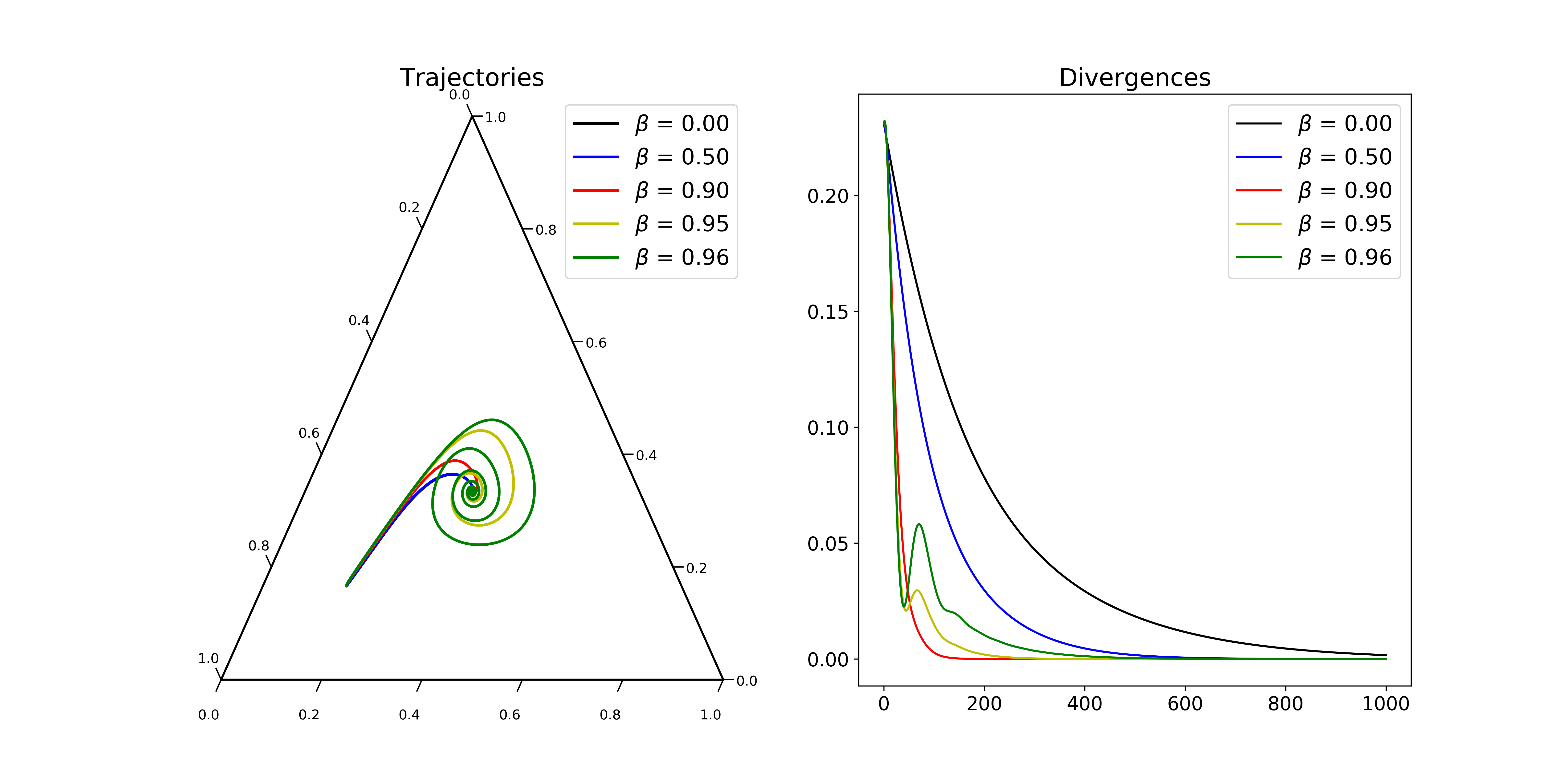
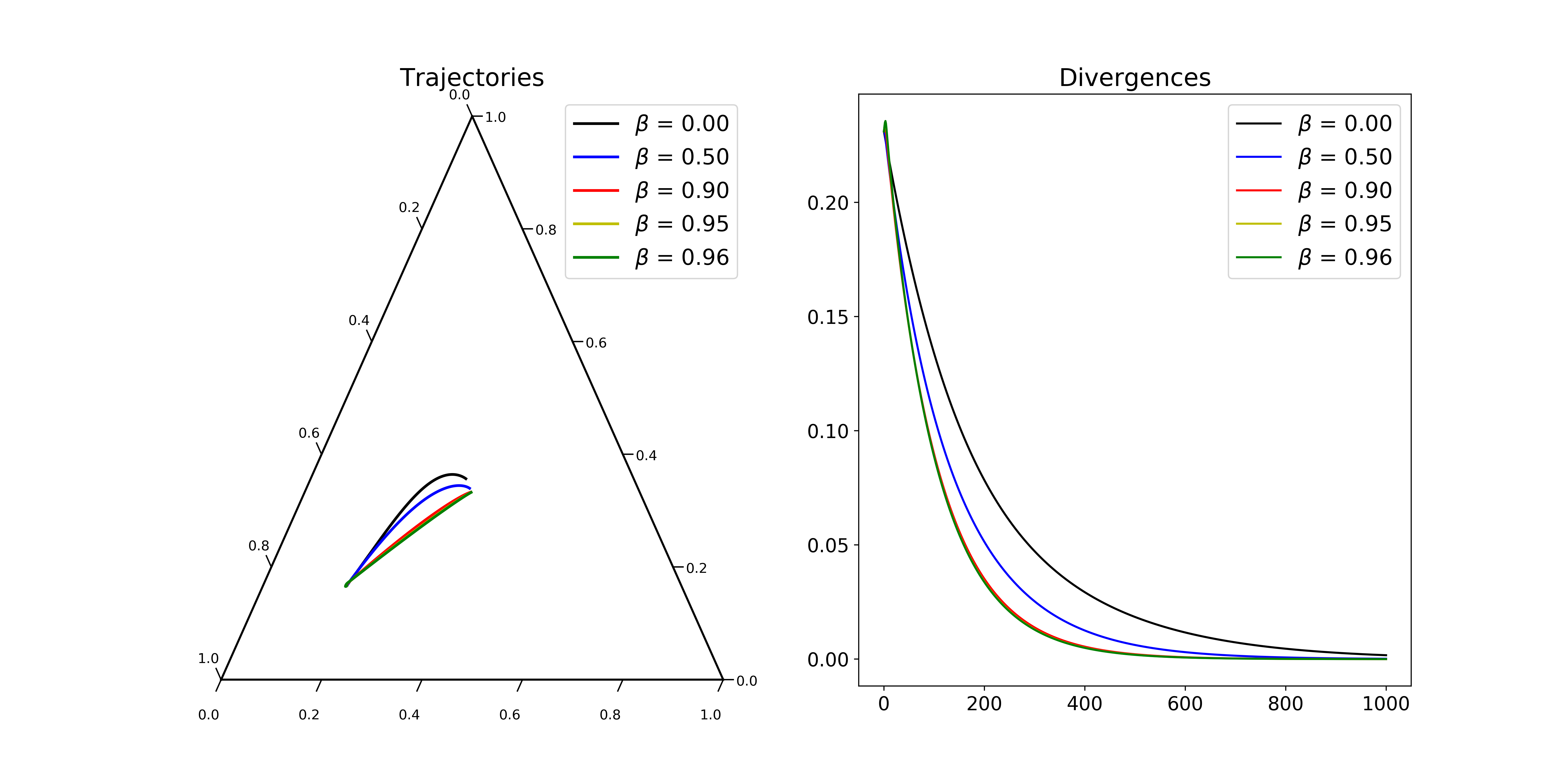
The proof of the theorem is straightforward and given in the appendix. We note that it holds for any learning rate $\alpha$, but the permissible values of $\beta$ may vary with both $\alpha$ and the fitness landscape. Below, we develop a similar result for the continuous dynamic (the limit that $\alpha\to 0$) which works for any $\beta\neq 1$. In general there cannot be a variant of Theorem 2 for Polyak momentum, arbitrary learning rate $\alpha$, and arbitrary momentum $\beta$: the hypothesis that at least one of $\alpha$ and $\beta$ is small is necessary (see examples in Figures 1 and 2).

Figure 1: Examples of altered convergence time for Polyak (top 2) and Nesterov (bottom 2) momentum. In all cases we use a landscape with $a=2$ and $b=1$ and $\alpha=1/200$. As $\beta$ increases, the dynamics typically converge faster, and the trajectories are not identical since $\alpha>0$. However, for Polyak momentum (top), as the value of $\beta$ becomes closer to 1, the Lyapunov quantity eventually fails to be monotonic along the entirety of the trajectory (it is at best local). Contrast with the Nesterov momentum trajectories (bottom) for the same parameters, which in this case are all monotonically decreasing.

Figure 2: For large values of momentum the dynamic may fail to converge as in the momentum free case if $\alpha$ is not sufficiently small. For all trajectories here $\alpha=0.01$, $a=2$, and $b=-1$. Lowering $\alpha$ to 0.001 restores convergence of the red $\beta=0.9$ curve.

4 Effect of Momentum on Rate of Convergence

While it’s good to know that the addition of some memory to the replicator equation does not alter the stable states, a more interesting effect is the acceleration of convergence. This is why momentum is of interest in machine learning. For evolutionary processes, this acceleration suggests one reason why epigenetic mechanisms may have evolved and persisted.

4.1 Time to Converge

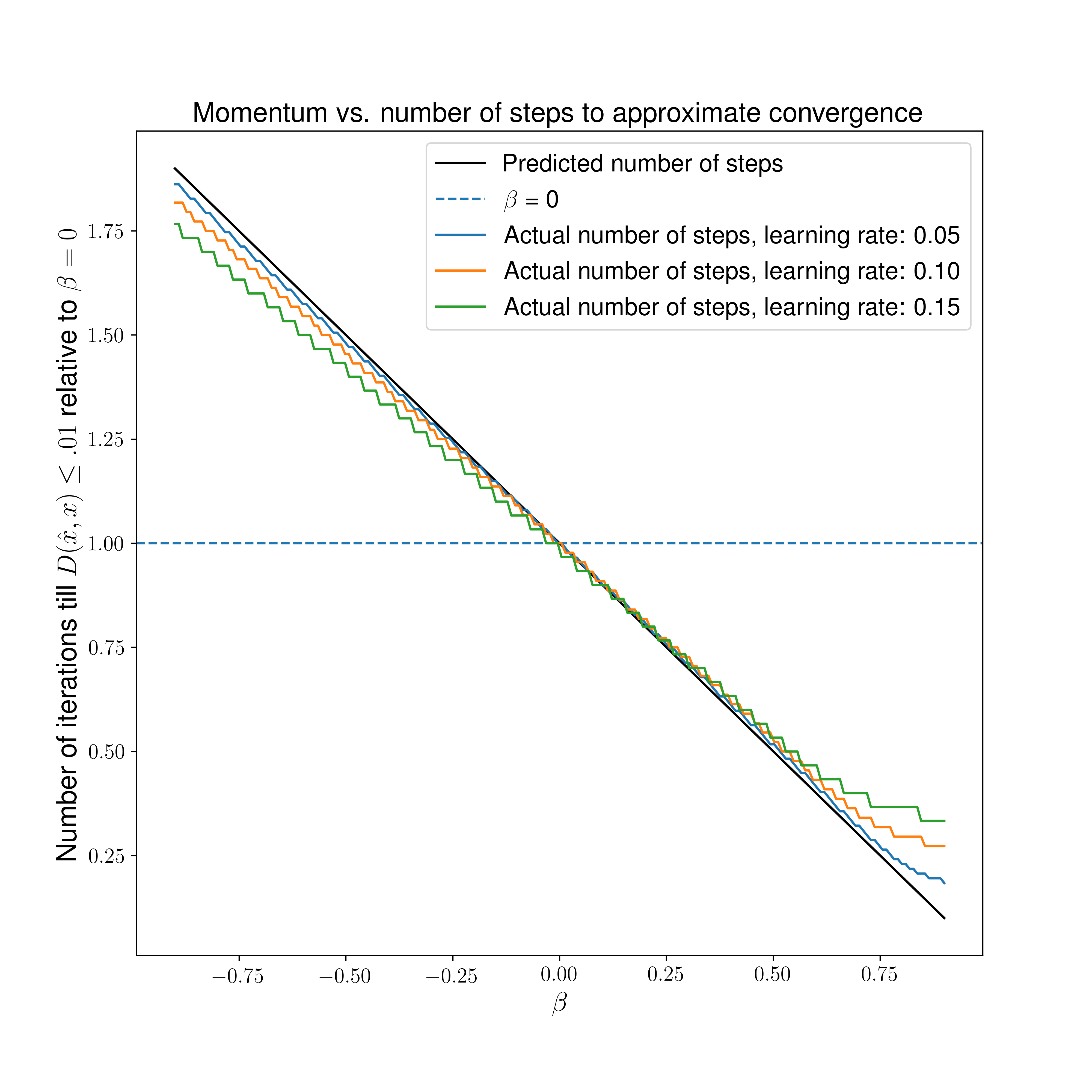
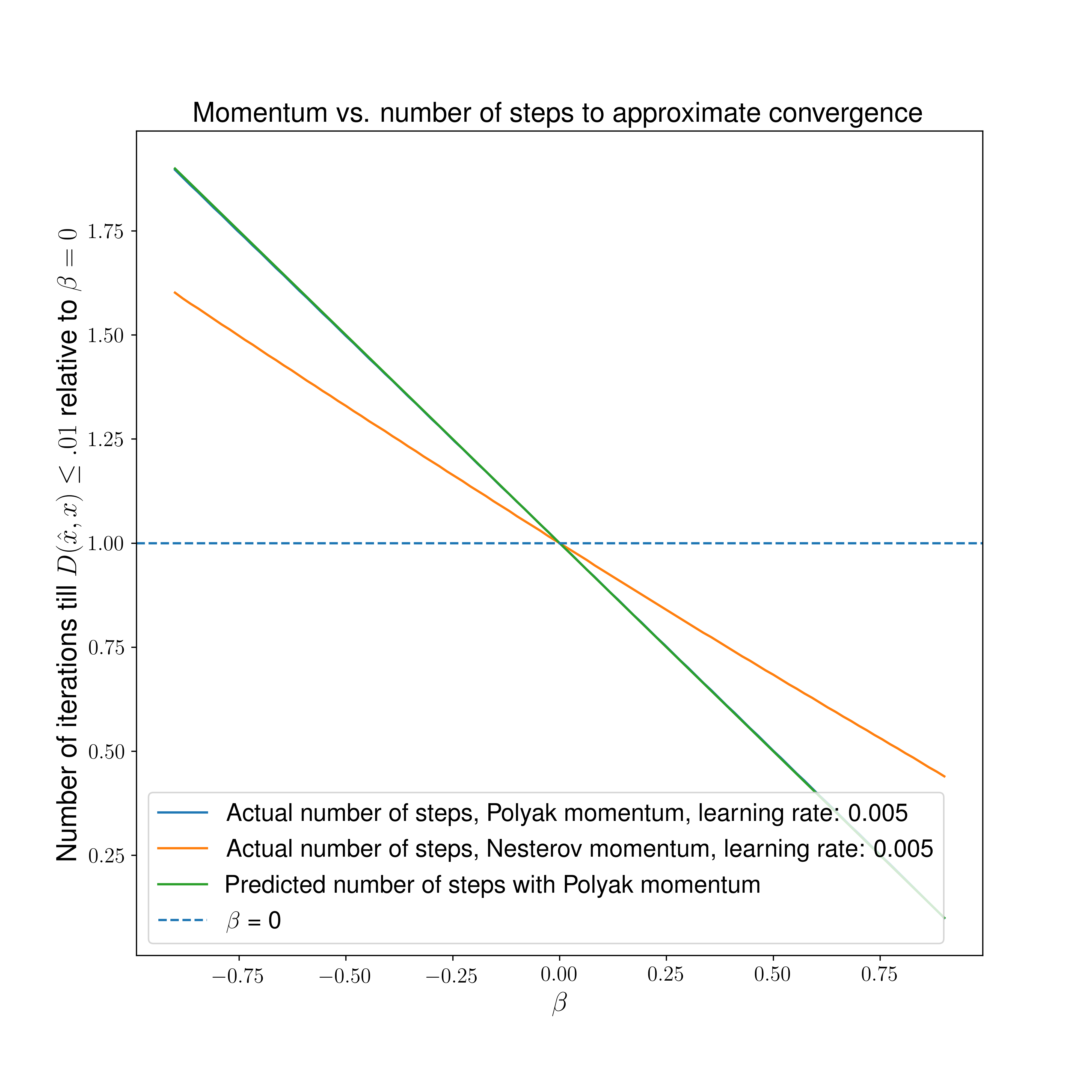
We can again use Lyapunov methods to see that the rate of convergence increases with momentum . Empirically we find that the convergence takes fewer steps by a factor of approximately $(1-\beta)$ of the momentum-free case, which we now demonstrate with an analytic argument. First we note that this factor makes sense intuitively given the iterative nature of momentum in Equation 3 since

$$\frac{1}{1-\beta}=1+\beta+\beta^{2}+\cdots$$

Now we hold momentum constant and allow the learning rate to converge to zero, yielding a continuous replicator dynamic with momentum associated to the discrete replicator dynamic, as follows. From Equation 3, as the discrete dynamic converges, we set $z_{i}^{\prime}=z_{i}$ to find that $z_{i}=\frac{F_{i}}{1-\beta}$. Letting $\alpha\to 0$ we obtain, after substituting in $z_{i}$ to the second equation

$$\frac{dx_{i}}{dt}=\frac{1}{1-\beta}x_{i}\left(f_{i}(x)-\bar{f}(x)\right)$$ (10)

where a factor of $1/\bar{f}(x)$ has been removed for brevity, corresponding to a scaling of time . Setting $\beta=0$ recovers the standard definition of the replicator equation just as in the discrete case. The leading factor of $1/(1-\beta)$ can similarly be eliminated by change of time scaling in the continuous case without altering the trajectories of the continuous dynamic, however we retain it to argue explicitly that the convergence rate increases as $\beta$ increases within $(0,1)$, increasing relative to the base case $\beta=0$ for $\beta\in(0,1)$. Similarly, the converge slows down for $\beta\in(-\infty,0)$. Note that traditionally in EGT, scaling the continuous replicator equation this way would not be considered particularly interesting since the trajectories (and stable points) do not change, however the increased rate of convergence is of paramount importance in machine learning (and perhaps to actual evolving populations).

Let $V_{\beta}=D(\hat{x},x_{\beta})$ be the KL-divergence with $\hat{x}$ an ESS and $x_{\beta}$ denoting that the trajectories evolve in time according to the replicator dynamic with momentum $\beta$ as in Equation 10. An easy calculation shows that

$$\frac{dV_{\beta}}{dt}=\frac{1}{1-\beta}\frac{dV_{0}}{dt}$$ (11)

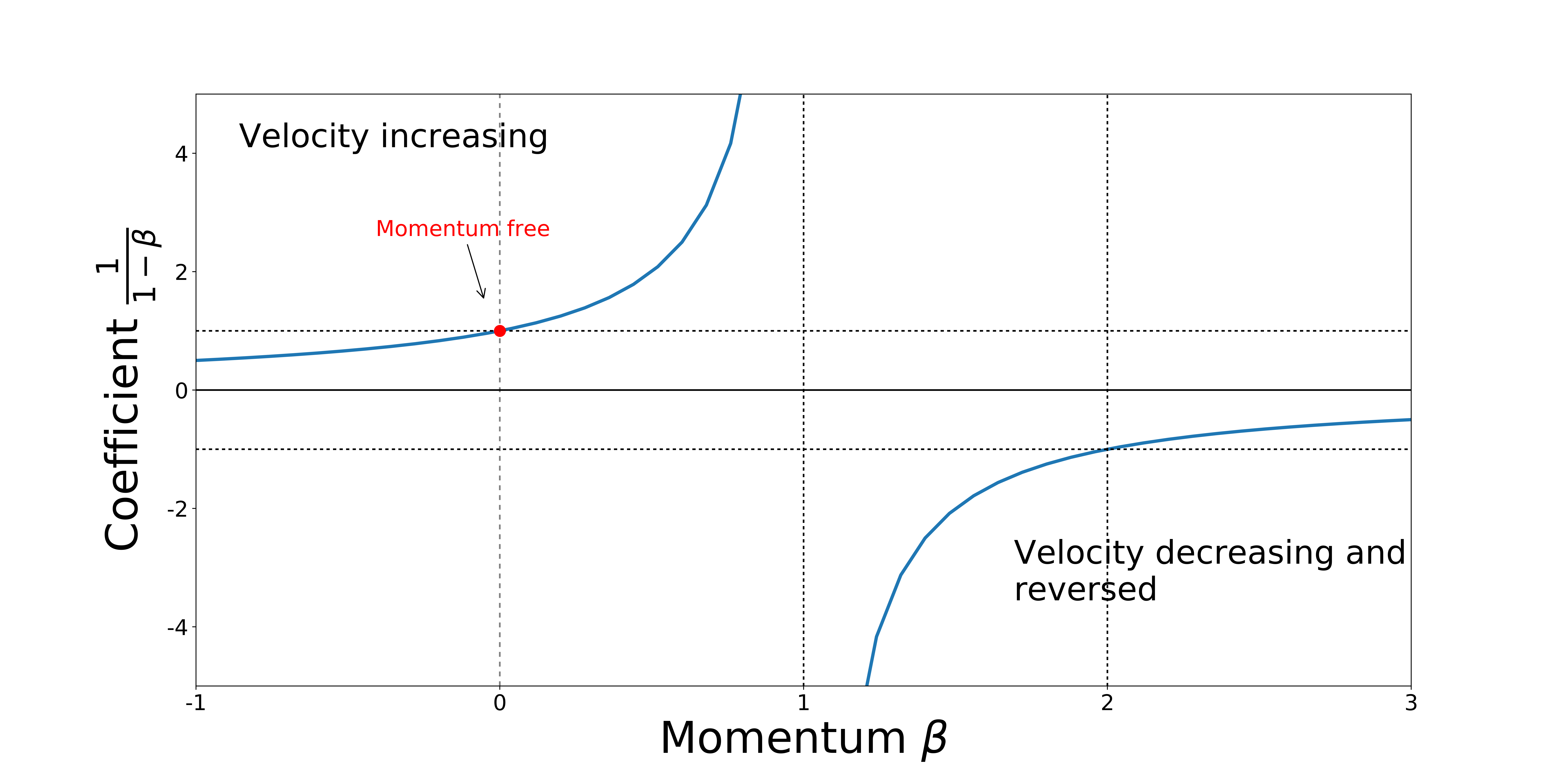
where we’ve used Equation 10 and the chain rule, i.e. we effectively scale the derivative of Lyapunov quantity by the leading factor. From this simple fact follows Theorem 3, which shows that the dynamic convergence and trajectory velocity is altered accordingly to $1/(1-\beta)$. The theorem is summarized in Figure 5 in the supplement.

Theorem 3.

Let $V_{\beta}$ be defined as above. Then we have that:

1. For $-\infty<\beta<1$, the ESS of the dynamic with (Polyak) momentum are the same as for the momentum free case; equivalently the KL-divergence is still a Lyapunov function for $\beta<1$.

2. For $1<\beta<\infty$, the directionality of the trajectory is reversed (so any ESS for $\beta<1$ is no longer an ESS)

3. The speed of the convergence is increasing on the intervals $(-\infty,1)$, and decreasing on $(1,\infty)$ (with direction reversed in the latter case)

4. In particular, the speed of convergence is faster than the momentum free dynamic for $0<\beta<1$ and the ESS are unchanged.

For the continuous dynamic, in the case that the dynamic converges to an ESS, Equation 11 also shows that it takes $\approx(1-\beta)$ as much time for the dynamic to be within $\epsilon$ of the ESS when compared to the momentum-free dynamic, as measured by the KL-divergence, starting from the same initial point. Thus the trajectories converge more quickly as $\beta$ ranges from 0 to 1, and the convergence slows for $\beta<0$.

Returning to the discrete dynamic, for continuous landscapes and smaller $\alpha$, we also roughly have that time-scale derivatives of the KL-divergence scale by $1/(1-\beta)$, though we cannot as easily compare directly along trajectories and the associated trajectories will not trace out the same curves (as seen in the examples above), so is there is not a direct analog of Equation 11. Nevertheless we may reasonably predict that it takes approximately $(1-\beta)$ as many steps as the momentum free case to be within $\epsilon$ of the ESS compared to the dynamic without momentum ($\beta=0$), demonstrated in the computational examples below. This approximation improves as the learning rate $\alpha\to 0$. Computationally we also find that the dynamic with Nesterov momentum exhibits a similar behavior (Figure 3). While the argument of Theorem 3 does not directly apply to Nesterov momentum, for small $\beta$ and continuous fitness landscape, a continuity argument suggests that the same approximation holds.

For completeness, we note that Theorem 3 also holds for the projection dynamic in an analogous manner, that is, to gradient descent on the Euclidean geometry, and should similarly apply to other Riemannian geometries as described in [34].

Theorem 4.

Theorem 3 also holds for the projection dynamic with the Lyapunov function $\frac{1}{2}||x-\hat{x}||^{2}$.

Figure 3: Left: Convergence speed up for Polyak momentum: Convergence time for small learning rates are well approximated by $(1-\beta)$ times the momentum free convergence time ($\beta=0$) of iterations for small learning rates. Right: The dynamic with Nesterov momentum is also fairly well approximated by a constant factor times the momentum free convergence time, but is clearly not scaled by the same factor. The fitness landscape is defined by $a=1=b$.

5 Momentum can break cycling into convergence or divergence

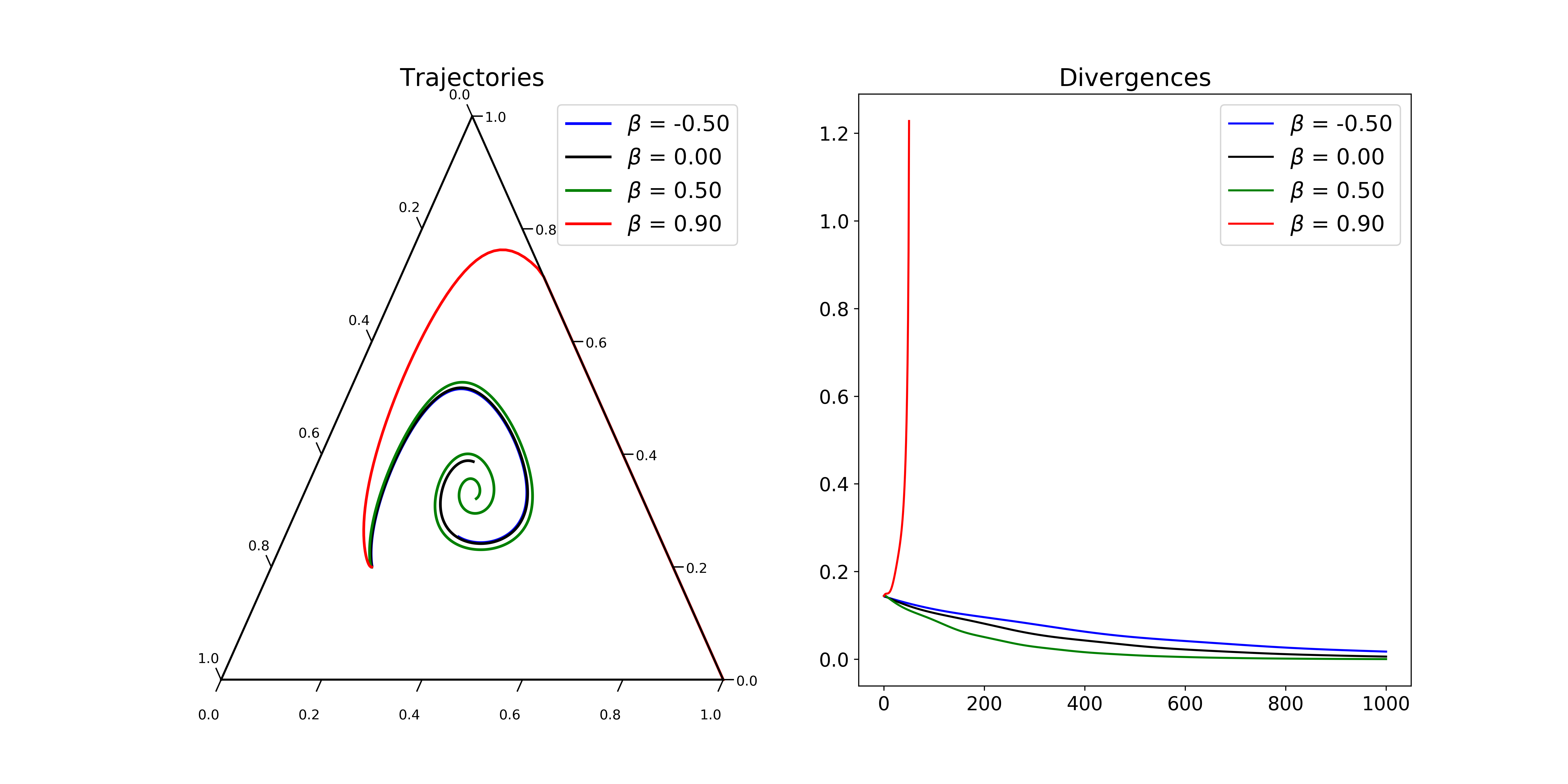
For the rock-paper-scissors landscape with $a=-b\neq 0$, the replicator equation is not a gradient. Since the mean fitness is zero (the game is zero-sum as the payoff matrix is skew-symmetric), the gradient flow is degenerate (the dynamic is motionless). However the replicator equation with this landscape is not degenerate and the phase portrait consists of concentric cycles of constant KL-divergence from the interior center of the simplex. The cycles are non-absorbing and the KL-divergence is an integral of motion. In the continuous case ($\alpha\to 0$), momentum alters the time to cycle around the central point, and possibly also reverses the directionality of the cycles, in accordance with the inequalities in Theorem 3.

In contrast, for non-zero learning rate $\alpha$, we find computationally that the momentum can cause the trajectories to converge inward or diverge outward. For Polyak momentum, the memory of the prior iterations causes the divergence, preventing the dynamic from turning sufficiently. For Nesterov momentum, it is the look-ahead aspect of the momentum that induces the convergence by causing the dynamic to turn more quickly.

Figure 4: For the rock-paper-scissors landscape ($a=1$, $b=-1$), momentum $\beta=0.65$, and learning rate $\alpha=1/200$, the replicator equation cycles indefinitely with constant KL-divergence based on the initial point. Adding momentum with a non-zero learning rate can cause the cycling to break into either convergence or divergence. In this case Nesterov momentum causes the dynamic to converge while Polyak momentum causes the dynamic to slowly diverge to the boundary.

6 Discussion

We’ve shown that momentum can accelerate evolutionary dynamics in the probability simplex just as it does for gradient descent in the machine learning literature. Lyapunov methods, commonly used to analyze dynamical systems but not yet as commonly applied in machine learning, allow us to show analytically and explicitly that momentum decreases the time to converge for values of momentum typically used in ML, and otherwise cause divergence or slowdown of trajectories for momentum outside of the interval $[0,1)$. Crucially we have shown that learning rate and momentum interact so that preservation of the convergence properties of the dynamic are guaranteed only for small $\beta$ or $\alpha$ despite the frequently realized speed up in convergence for larger values of momentum.

Interpreting the results, we’ve shown that the convergence of evolutionary dynamics can be accelerated by a mechanism of memory that can be viewed as a simple model of intergenerational information exchange such as epigentics. This may also apply to immunity or cultural exchanges of information and explain the origin and persistence of extra-genetic information exchange in lineages and populations.

6.1 Code

The code to generate the trajectories and plots in this manuscript is available as a Python library pyed at https://github.com/marcharper/pyed. Ternary plots were generated with the python-ternary library [41].

Broader Impact discussion

This work provides theoretical insight into the nature of momentum and connections between models of evolution and machine learning algorithms. The authors anticipate no specific immediate ethical implications or societal impacts. This work may ultimately lead to more efficient machine learning methods and evolutionary processes, which could have positive or negative consequences depending on the specific application.

7 Supplemental Material

7.1 Graphical depiction of Theorem 3

Figure 5: Graphical depiction of Theorem 3 in terms of the properties of the dynamic coefficient $\frac{1}{1-\beta}$. As $\beta$ varies the convergence and trajectory velocity changes in accordance with the coefficient $1/(1-\beta)$. The trajectory velocity is increasing with $\beta$ on $(-\infty,1)$ and $(1,\infty)$, the orientation is reversed on $(1,\infty)$, and the velocity is faster than the momentum free case ($\beta=0$) for $(0,1)$ and $(1,2)$.

7.2 Proof of Equation 11

Taking the derivative of the KL-divergence, using the definition of the continuous replicator equation, gives the following:

$$\frac{d}{dt}D(\hat{x}||x) =-\sum_{i}{\frac{\hat{x}_{i}}{x_{i}}\frac{dx_{i}}{dt}}$$

$$=-\sum_{i}{\hat{x}_{i}(f_{i}-\bar{f})}$$

$$=x\cdot f-\hat{x}\cdot f$$

This quantity is less than zero if $\hat{x}$ is an evolutionarily stable state (which proves Theorem 1 in the continuous case). If we instead use the replicator equation with momentum (Equation 10), a factor of $\frac{1}{1-\beta}$ is present on the right hand side of the equation above, proving Equation 11.

7.3 Proof of Theorem 2

Proof.

Since the KL-divergence is positive and zero only at $\hat{x}$, essentially one just needs to show that the quantity

$$D^{\Delta}(x)=\frac{D(\hat{x}||x^{\prime})-D(\hat{x}||x)}{\alpha}$$

is less than zero when $\hat{x}$ is an ESS (for fixed $\alpha$) to establish it as a discrete Lyapunov function.

A straightforward algebraic calculation shows that this quantity is bounded by

$$-\log\left(\sum_{i}\hat{x}_{i}\frac{x_{i}^{\prime}}{x_{i}}\right)=-\log\left(1+\alpha\beta\sum_{i}{\frac{\hat{x}_{i}z_{i}}{x_{i}}}+\alpha\left(\frac{\hat{x}\cdot f}{x\cdot f}-1\right)\right)$$

which is less than 0 for sufficiently small $\beta$ and the inequality defining an ESS. ∎

When $\alpha\to 0$ it’s easier to directly use ordinary differentiation to prove the continuous version of Theorem 2. Proof for the projection dynamic using the Euclidean distance is analogous and omitted. In the case of Nesterov momentum, continuity of the fitness landscape and small $\beta$ reduces to the Polyak momentum case.

References

- [1] David E Goldberg and John Henry Holland. Genetic algorithms and machine learning. Machine Learning, 3, 1988.
- [2] David E Moriarty, Alan C Schultz, and John J Grefenstette. Evolutionary algorithms for reinforcement learning. Journal of Artificial Intelligence Research, 11:241–276, 1999.
- [3] Tim Salimans, Jonathan Ho, Xi Chen, Szymon Sidor, and Ilya Sutskever. Evolution strategies as a scalable alternative to reinforcement learning. arXiv preprint arXiv:1703.03864, 2017.
- [4] Thomas Elsken, Jan Hendrik Metzen, and Frank Hutter. Neural architecture search: A survey. arXiv preprint arXiv:1808.05377, 2018.
- [5] Esteban Real, Chen Liang, David R So, and Quoc V Le. Automl-zero: Evolving machine learning algorithms from scratch. arXiv preprint arXiv:2003.03384, 2020.
- [6] Chrisantha Fernando, Jakub Sygnowski, Simon Osindero, Jane Wang, Tom Schaul, Denis Teplyashin, Pablo Sprechmann, Alexander Pritzel, and Andrei Rusu. Meta-learning by the baldwin effect. In Proceedings of the Genetic and Evolutionary Computation Conference Companion, pages 1313–1320, 2018.
- [7] Chris Murgatroyd, Alexandre V Patchev, Yonghe Wu, Vincenzo Micale, Yvonne Bockmühl, Dieter Fischer, Florian Holsboer, Carsten T Wotjak, Osborne FX Almeida, and Dietmar Spengler. Dynamic dna methylation programs persistent adverse effects of early-life stress. Nature neuroscience, 12(12):1559, 2009.
- [8] Mark Pagel. Human language as a culturally transmitted replicator. Nature Reviews Genetics, 10(6):405, 2009.
- [9] Milton J Schlesinger. Heat shock proteins. Journal of Biological Chemistry, 265(21):12111–12114, 1990.
- [10] Peter D Taylor and Leo B Jonker. Evolutionary stable strategies and game dynamics. Mathematical biosciences, 40(1-2):145–156, 1978.
- [11] Ning Qian. On the momentum term in gradient descent learning algorithms. Neural networks, 12(1):145–151, 1999.
- [12] Ilya Sutskever, James Martens, George Dahl, and Geoffrey Hinton. On the importance of initialization and momentum in deep learning. In International conference on machine learning, pages 1139–1147, 2013.
- [13] Gabriel Goh. Why momentum really works. Distill, 2(4):e6, 2017.
- [14] Yu Nesterov. A method of solving a convex programming problem with convergence rate . Sov. Math. Dokl, 27(2), 1983.
- [15] Weijie Su, Stephen Boyd, and Emmanuel J Candes. A differential equation for modeling nesterov’s accelerated gradient method: theory and insights. The Journal of Machine Learning Research, 17(1):5312–5354, 2016.
- [16] Hongyi Zhang and Suvrit Sra. Towards riemannian accelerated gradient methods. arXiv preprint arXiv:1806.02812, 2018.
- [17] Kwangjun Ahn and Suvrit Sra. From nesterov’s estimate sequence to riemannian acceleration. arXiv preprint arXiv:2001.08876, 2020.
- [18] Aaron Defazio. On the curved geometry of accelerated optimization. In Advances in Neural Information Processing Systems, pages 1764–1773, 2019.
- [19] Yuzuru Sato, Eizo Akiyama, and James P Crutchfield. Stability and diversity in collective adaptation. Physica D: Nonlinear Phenomena, 210(1-2):21–57, 2005.
- [20] Gauthier Gidel, Reyhane Askari Hemmat, Mohammad Pezeshki, Gabriel Huang, Remi Lepriol, Simon Lacoste-Julien, and Ioannis Mitliagkas. Negative momentum for improved game dynamics. arXiv preprint arXiv:1807.04740, 2018.
- [21] Dale Schuurmans and Martin A Zinkevich. Deep learning games. In Advances in Neural Information Processing Systems, pages 1678–1686, 2016.
- [22] David Balduzzi, Sebastien Racaniere, James Martens, Jakob Foerster, Karl Tuyls, and Thore Graepel. The mechanics of n-player differentiable games. arXiv preprint arXiv:1802.05642, 2018.
- [23] John Baez and Blake Pollard. Relative entropy in biological systems. Entropy, 18(2):46, 2016.
- [24] Zbigniew Bartosiewicz and Ewa Piotrowska. Lyapunov functions in stability of nonlinear systems on time scales. Journal of Difference Equations and Applications, 17(03):309–325, 2011.
- [25] Euhanna Ghadimi, Hamid Reza Feyzmahdavian, and Mikael Johansson. Global convergence of the heavy-ball method for convex optimization. In 2015 European Control Conference (ECC), pages 310–315. IEEE, 2015.
- [26] Boris T Polyak. Some methods of speeding up the convergence of iteration methods. USSR Computational Mathematics and Mathematical Physics, 4(5):1–17, 1964.
- [27] Ross Cressman and Yi Tao. The replicator equation and other game dynamics. Proceedings of the National Academy of Sciences, 111(Supplement 3):10810–10817, 2014.
- [28] Siavash Shahshahani. A new mathematical framework for the study of linkage and selection. American Mathematical Soc., 1979.
- [29] Akio Fujiwara and Shun-ichi Amari. Gradient systems in view of information geometry. Physica D: Nonlinear Phenomena, 80(3):317–327, 1995.
- [30] Shun-Ichi Amari. Natural gradient works efficiently in learning. Neural computation, 10(2):251–276, 1998.
- [31] Bolin Gao and Lacra Pavel. On the properties of the softmax function with application in game theory and reinforcement learning. arXiv preprint arXiv:1704.00805, 2017.
- [32] Ashia C Wilson, Benjamin Recht, and Michael I Jordan. A lyapunov analysis of momentum methods in optimization. arXiv preprint arXiv:1611.02635, 2016.
- [33] Ashia Wilson. Lyapunov arguments in optimization. University of California, Berkeley, 2018.
- [34] Marc Harper and Dashiell Fryer. Lyapunov functions for time-scale dynamics on riemannian geometries of the simplex. Dynamic Games and Applications, 5(3):318–333, 2015.
- [35] John Maynard Smith. Evolution and the Theory of Games. Cambridge university press, 1982.
- [36] Immanuel M Bomze. Cross entropy minimization in uninvadable states of complex populations. Journal of Mathematical Biology, 30(1):73–87, 1991.
- [37] Ethan Akin and Viktor Losert. Evolutionary dynamics of zero-sum games. Journal of mathematical biology, 20(3):231–258, 1984.
- [38] Anna Nagurney and Ding Zhang. Projected dynamical systems in the formulation, stability analysis, and computation of fixed-demand traffic network equilibria. Transportation Science, 31(2):147–158, 1997.
- [39] Ratul Lahkar and William H Sandholm. The projection dynamic and the geometry of population games. Games and Economic Behavior, 64(2):565–590, 2008.
- [40] Marc Harper. Escort evolutionary game theory. Physica D: Nonlinear Phenomena, 240(18):1411–1415, 2011.
- [41] Marc Harper et al. python-ternary: Ternary plots in python. Zenodo 10.5281/zenodo.594435, 2020.