Pretrained Generalized Autoregressive Model with Adaptive Probabilistic
Label Clusters for Extreme Multi-label Text Classification

Abstract

Extreme multi-label text classification (XMTC) is a task for tagging a given text with the most relevant labels from an extremely large label set. We propose a novel deep learning method called APLC-XLNet. Our approach fine-tunes the recently released generalized autoregressive pretrained model (XLNet) to learn a dense representation for the input text. We propose Adaptive Probabilistic Label Clusters (APLC) to approximate the cross entropy loss by exploiting the unbalanced label distribution to form clusters that explicitly reduce the computational time. Our experiments, carried out on five benchmark datasets, show that our approach has achieved new state-of-the-art results on four benchmark datasets. Our source code is available publicly at https://github.com/huiyegit/APLC_XLNet.

1 Introduction

Extreme classification is the problem of learning a classifier to annotate each instance with the most relevant labels from an extremely large label set. Extreme classification has found applications in diverse areas, such as estimation of word representations for millions of words (Mikolov et al., 2013), tagging of a Wikipedia article with the most relevant labels (Dekel & Shamir, 2010), and providing a product description or an ad-landing page in Dynamic Search Advertising (Jain et al., 2019). Extreme multi-label text classification (XMTC) is a fundamental task of extreme classification where both the instances and labels are in text format.

The first challenge of XMTC is how to get effective features to represent the text. One traditional approach to represent text features is bag-of-words (BOW), where a vector represents the frequency of a word in a predefined vocabulary. Then, the machine learning algorithm is fed with training data that consists of pairs of features and labels to train a classification model. Nevertheless, the traditional methods based on BOW or its variants, ignoring the location information of the words, cannot capture the contextual and semantic information of the text.

On the other hand, with the recent development of word embedding techniques, deep learning methods have achieved great success for learning text representation from raw text. These effective models include the Convolutional Neural Network (CNN) (Kim, 2014), the Recurrent Neural Network (RNN) (Liu et al., 2016), the combination of CNN and RNN (Lai et al., 2015) , the CNN with Attention mechanism (Yin & Schütze, 2018), the RNN with Attention mechanism (Yang et al., 2016) and the Transformer (Vaswani et al., 2017; Guo et al., 2019).

Over the last two years, several transfer learning methods and architectures (Devlin et al., 2019; Radford et al., 2018; Conneau & Lample, 2019; Yang et al., 2019b) have been proposed, and have achieved state-of-the-art results on a wide range of natural language processing (NLP) tasks, including question answering (Yang et al., 2019a), sentiment analysis (Xu et al., 2019), text classification (Sun et al., 2019) and information retrieval (Chen et al., 2020). The basic mechanism of transfer learning is to transfer the knowledge of a pretrained model, generally trained on very large corpora, into a new downstream task. The generalized autoregressive pretraining method (XLNet) (Yang et al., 2019b) represents the latest development in this field. XLNet adopts the permutation language modeling objective to train the model on several large corpora. Then the pretrained model can be fine-tuned to deal with various NLP tasks.

Another challenge of XMTC is how to handle the extreme outputs efficiently. In particular, for extreme classification, the distribution of the labels notoriously follows Zipf’s Law. Most of the probability mass is covered by only a small fraction of the label set. To train parametric models for language modeling with very large vocabularies, many methods have been proposed to approximate the softmax efficiently, including Hierarchical Softmax (HSM) (Morin & Bengio, 2005), Negative Sampling (Mikolov et al., 2013), Noise Contrastive Estimation (Mnih & Teh, 2012; Vaswani et al., 2013) and Adaptive Softmax (Grave et al., 2017). However, these techniques are proposed to deal with multi-class classification, so they can not be applied to XMTC directly. The Probabilistic Label Tree (PLT) (Jasinska et al., 2016; Wydmuch et al., 2018) generalizes the HSM to handle the multi-label classification problem.

Motivated by these characteristics of the task, we present a novel deep learning approach, Pretrained Generalized Autoregressive Model with Adaptive Probabilistic Label Clusters (APLC-XLNet). We fine-tune the generalized autoregressive pretraining model (XLNet) to learn the powerful text representation to achieve high prediction accuracy. To the best of our knowledge, XLNet is the first time to be applied successfully to the XMTC problem. Inspired by the Adaptive Softmax, we propose the Adaptive Probabilistic Label Clusters (APLC) to approximate the cross entropy loss by exploiting the unbalanced label distribution to form clusters that explicitly reduce computation time. APLC can be flexible enough to achieve the desirable balance between the prediction accuracy and computation time by adjusting its parameters. Furthermore, APLC can be general enough to deal with the extreme classification problem efficiently as the output layer. The experiments, conducted on five datasets, have demonstrated that our approach has achieved new state-of-the-art results on four benchmark datasets.

2 Related Work

Many effective methods have been proposed for addressing the challenges of XMTC. They can be generally categorized into two types according to the method used for feature representation. One traditional type is to use the BOW as the feature. It contains three different approaches: one-vs-all approaches, embedding-based approaches and tree-based approaches. The other type is the modern deep learning approach. Deep learning models have been proposed to learn powerful text representation from the raw text and have shown great success on different NLP tasks.

One-vs-all approaches. The one-vs-all approaches treat each label independently as a binary classification problem that learns a classifier for each label. The one-vs-all approaches have been shown to achieve high accuracy, but they suffer from expensive computational complexity when the number of labels is very large. PDSparse (Yen et al., 2016) learns a separate linear classifier per label. During training, the classifier is optimized to distinguish between all the positive labels and a few active negative labels of each training sample. PPDSparse (Yen et al., 2017) extends PDSparse to be parallelized in large scale distributed settings. DiSMEC (Babbar & Schölkopf, 2017) presents a distributed and parallel training mechanism, which can exploit as many computation cores as are available. In addition, it can reduce the model size by explicitly inducing sparsity via pruning of spurious weights. Slice (Jain et al., 2019) trains each label’s classifier over the most confusing negative labels rather than all the negative labels. This is achieved efficiently by a novel negative sampling technique.

Embedding-based approaches. Embedding-based approaches project the high-dimensional label space into a low-dimensional one by exploiting label correlations and sparsity. Embedding methods may pay a heavy price in terms of prediction accuracy due to the loss of information in the compression phase. SLEEC (Bhatia et al., 2015) projects the high-dimensional label space into the low-dimensional one by preserving the pairwise distances between only the closest label vectors. The regressors can be learned over the low-dimensional label space. AnnexML (Tagami, 2017) partitions data points by using an approximate k-nearest neighbor graph as weak supervision. Then it employs a pairwise learning-to-rank approach to learn the low-dimensional label space.

Tree-based approaches. Tree-based methods learn a hierarchical tree structure to partition the instances or labels into different groups so that similar ones can be in the same group. The whole set, initially assigned to the root node, is partitioned into a fixed number k subsets corresponding to k child nodes of the root node. The partition process is repeated until a stopping condition is satisfied on the subsets. In the prediction phase, the input instance passes down the tree until it reaches the leaf node. For an instance tree, the prediction is given by the classifier trained on the leaf instances. For a label tree, the prediction of a given label is the probability determined by the traversed node classifiers from the root node to the leaf node.

FastXML (Prabhu & Varma, 2014) learns a tree structure over the feature space by optimizing the normalized Discounted Cumulative Gain (nDCG). A binary classifier is trained for each internal node. The prediction for a given instance is the label distribution which is computed over the training instances in the corresponding leaf node. Based on FastXML, PfastreXML (Jain et al., 2016) introduces propensity scored losses which prioritize predicting the few relevant labels over the large number of irrelevant ones and promotes the prediction of infrequent, but rewarding tail labels. Parabel (Prabhu et al., 2018) learns a ensemble of three label trees. The label tree is trained by recursively partitioning the labels into two balanced groups. The leaf nodes contain linear one-vs-all classifiers, one for each label in the leaf. The one-vs-all classifiers are used to compute the probability of the corresponding labels relevant to the test point.

CRAFTML (Siblini et al., 2018) introduces a random forest-based method with a fast partitioning strategy. At first, it randomly projects both the feature and label vectors into low-dimensional vectors. Then a k-means based partitioning method splits the instances into k temporary subsets from the low-dimensional label vectors. A multi-class classifier in the internal node can be trained for its relevant subset from the low-dimensional feature vectors. Bonsai (Khandagale et al., 2019) develops a generalized label representation by combining the input and output representations. Then it constructs a shallow tree architecture through the k-means clustering. Bonsai has demonstrated fast speed to deal with an extremely large dataset. ET (Wydmuch et al., 2018) adopts the same architecture as FastText (Joulin et al., 2017), but it employs the Probabilistic Label Tree as the output layer to deal with the multi-label classification instead of the Hierarchical Softmax. ET has the advantages of small model size and efficient prediction time. However, since the architecture of FastText cannot capture the rich contextual information of the text, the prediction accuracy cannot be high.

Deep learning approaches. In contrast to BOW used by the traditional methods as the text representation, the raw text has been effectively utilized by deep learning models to learn the dense representation, which can capture the contextual and semantic information of the text. Based on CNN-Kim (Kim, 2014), XML-CNN (Liu et al., 2017) learns a number of feature representations by passing the text through convolution layers. A hidden bottleneck layer is added between the pooling and output layer to improve the prediction accuracy and reduce the model size. However, since the output layer of XML-CNN is a linear structure, it can be inefficient when applied to a case with millions of labels.

Inspired by the information retrieval (IR) perspective, X-BERT (Wei-Cheng et al., 2019) presents a method in three steps. At first, it builds the label indexing system by partitioning the label set into k clusters. Then it fine-tunes the Bidirectional Encoder Representations from Transformers (BERT) (Devlin et al., 2019) model to match label clusters for the input texts. In the last step, the linear classifiers are trained to rank the labels in the corresponding cluster. X-BERT fine-tunes the BERT model successfully and has shown significant improvement in terms of prediction accuracy. However, X-BERT is not an entire end-to-end deep learning model, so it leaves potential room to improve the results. AttentionXML (You et al., 2019) captures the sequential information of the text by the Bidirectional Long Short-term Memory (BiLSTM) model and the Attention mechanism. A shallow and wide probabilistic label tree is proposed to handle the large scale of labels. AttentionXML achieves outstanding performance on both accuracy and efficiency. However, an ensemble of three probabilistic label trees is adopted to improve the prediction accuracy, which is unusual in deep learning approaches.

3 APLC-XLNet

In this section, we elaborate on our APLC-XLNet model for the XMTC problem. Our model architecture has three components: the XLNet module, the hidden layer and the APLC output layer (Figure 1).

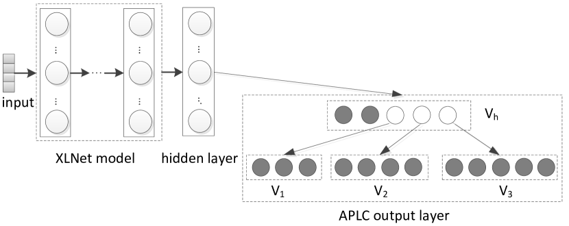
Figure 1: Architecture of the proposed APLC-XLNet model. $V$ denotes the label cluster in APLC.

3.1 XLNet module

Recently, there have been many significant advances in transfer learning for NLP, most of which are based on language modeling (Devlin et al., 2019; Radford et al., 2018; Conneau & Lample, 2019; Yang et al., 2019b). Language modeling is the task of predicting the next word in a sentence given previous words. XLNet (Yang et al., 2019b) is a generalized autoregressive pretraining language model that captures bidirectional contexts by maximizing the expected likelihood over all permutations of the factorization order. Its permutation language modeling objective can be expressed as follows:

$$\max_{\theta}E_{z\sim Z_{T}}\left[\sum_{t=1}^{T}log\>p_{\theta}\left(x_{z_{t}}|x_{z<t}\right)\right]$$ (1)

where $\theta$ denotes the parameters of the model, $Z_{T}$ is the set of all possible permutations of the sequence with length T, $z_{t}$ is the t-th element and $z<t$ deontes the preceding $t-1$ elements in a permutation $z$. Essentially, for a text sequence $x$, a factorization order $z$ can be sampled at one time, then the likelihood $p_{\theta}(x)$ can be obtained by decomposing this order.

In addition to permutation language modeling, XLNet adopts the Transformer XL (Dai et al., 2019) as its base architecture. XLNet pretrained the language model on a large corpus of text data, and then fine-tuned the pretrained model on downstream tasks. While the pretrained model has achieved state-of-the-art performance on many downstream tasks including sentence classification, question answering and sequence tagging, it remains unexplored for the application of extreme multi-label text classification.

We adopt the pretrained XLNet-Base model in our model architecture and fine-tune it to learn the powerful representation of the text. Following the approach of XLNet (Yang et al., 2019b), we begin with the pretrained XLNet model with one embedding layer, then the module consisting of 12 Transformer blocks. We take the final hidden vector of the last token corresponding to the special [CLS] token as the text representation.

3.2 Hidden layer

APLC-XLNet has one fully connected layer between the pooling layer of XLNet and APLC output layer. We choose to set the number of neurons in this layer as a hyperparameter $d_{h}$. When the number of output labels is not large, $d_{h}$ can be the same as the pooling layer to obtain the best text representation. On the other hand, when handling the case of extreme labels, it can be less than the pooling layer to largely reduce the model size and make the computation more efficient. In this case, this layer can be referred to as a bottleneck layer, as the number of neurons is less than both the pooling layer and output layer.

3.3 Adaptive Probabilistic Label Clusters

Motivation. In extreme classification, the distribution of the labels notoriously follows Zipf’s Law. Most of the probability mass is covered by only a small fraction of the label set. In one benchmark dataset, Wiki-500k, the frequent labels account for 20% of the label vocabulary, but they cover about 75% of probability mass (as shown in Figure 2). Similar to Hierarchical Softmax (Mikolov et al., 2011) and Adaptive Softmax (Grave et al., 2017), this attribute can be exploited to reduce the computation time.

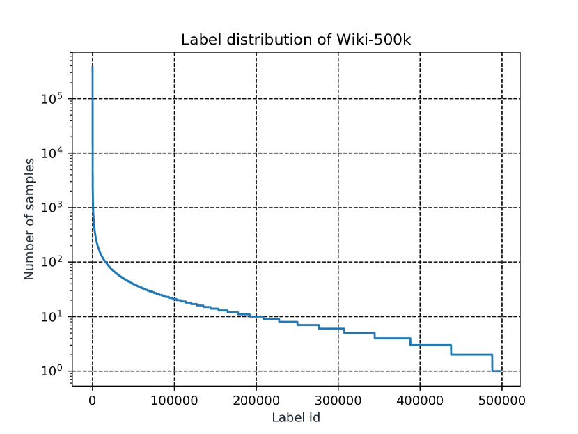
Figure 2: Label distribution of dataset Wiki-500k follows Zipf’s Law. Label ids are sorted in descending order by the number of occurrence in the dataset.

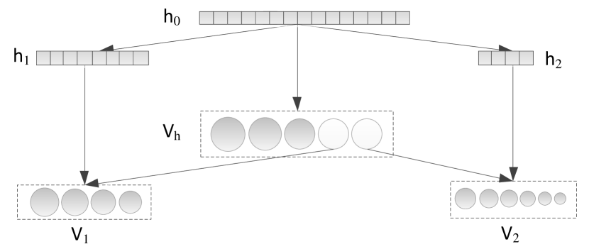
Figure 3: Architecture of the 3-cluster APLC. $h$ denotes the hidden state. $V_{h}$ denotes the head cluster. $V_{1}$ and $V_{2}$ denote the two tail clusters. The size of the leaf node indicates the frequency of the label.

Architecture. We partition the label set into a head cluster and several tail clusters, where the head cluster consists of the most frequent labels and the infrequent labels are grouped into the tail clusters (Figure 3). The head cluster containing a small fraction of labels corresponds to less computation time, so it would improve the efficiency of computation greatly by accessing it frequently. The structure of clusters can be developed in two different ways. One way is to generate a 2-level tree (Mikolov et al., 2011), while the other is to keep the head cluster as a short-list in the root node (Le et al., 2011; Grave et al., 2017). Empirically, it leads to a considerate decrease of performance to put all the clusters in the leaves. Like the Adaptive Softmax (Grave et al., 2017), we choose to put the head cluster in the root node. To further reduce the computation time, we adopt decreasing dimensions of hidden state as the inputs to the clusters. For the head cluster accessed by the classifier frequently, a large dimension of hidden state can keep the high prediction accuracy. For the tail clusters, since the classifier would access them infrequently, we decrease the dimension through dividing by the factor $q$ ($q\geq 1$). In this way, the model size of the clusters can be significantly reduced, yet the model can still maintain good performance.

Objective function. We assume the label set is partitioned as $V=V_{h}\cup V_{1}\cup\ldots\cup V_{K}$, where $V_{h}$ is the head cluster, $V_{i}$ is the i-th tail cluster,   $V_{h}\cap V_{i}=\emptyset\>\;\text{and}\>\;V_{i}\cap V_{j}=\emptyset,\>\text{if}\>i\neq j$, $K$ is the number of tail clusters. By the chain rule of probability, the probability of one label can be expressed as follows:

$$p(y_{j}|x)=\begin{cases}p(y_{j}|x),&\text{if $y_{j}\in V_{h}$}\\ p(V_{t}|x)p(y_{j}|V_{t},x),&\text{if $y_{j}\in V_{t}$}\end{cases}$$ (2)

where $x$ is the feature of one sample, $y_{j}$ is the j-th label, $V_{t}$ is the t-th tail cluster.

During training, we access the head cluster, where we compute the probability of each label for each training sample. In contrast, we access the tail cluster $V_{t}$, where we compute the probability of each label only if there is a positive label of the training sample located in $V_{t}$. Let $Y_{i}$ be the set of positive labels of the i-th instance, $V_{y_{k}}$ is the corresponding cluster of the k-th label in $Y_{i}$, the set of clusters $S_{i}$ corresponding to $Y_{i}$ can be expressed as follows:

$$S_{i}=\bigcup_{y_{k}\in Y_{i}}V_{y_{k}}$$ (3)

Note that $S_{i}$ can either contain or not contain the head cluster $V_{h}$, but we need to access $V_{h}$ for each training sample. We add $V_{h}$ into $S_{i}$ and the set of clusters $\hat{S_{i}}$ corresponding to $Y_{i}$ can be expressed as follows:

$$\hat{S_{i}}=S_{i}\bigcup V_{h}=(\bigcup_{y_{k}\in Y_{i}}V_{y_{k}})\bigcup V_{h}$$ (4)

Let $\hat{Y_{i}}$ be the label set corresponding to $\hat{S_{i}}$. We use $L_{i}$ to denote the cardinality of $\hat{Y_{i}}$, and $I_{i}$ denote the set of label indexes of $\hat{Y_{i}}$. The objective loss function of APLC for multi-label classification can be expressed as follows:

$$J(\theta)=-\frac{1}{\sum_{i=1}^{N}L_{i}}\sum_{i=1}^{N}\sum_{j\in I_{i}}(y_{ij}log\>p(y_{ij})+\\ (1-y_{ij})log\>(1-p(y_{ij})))$$ (5)

where N is the number of samples, $p(y_{ij})$ is the predicted probability computed from Equation 2, $y_{ij}\in\{0,1\}$ is the true value, index i and j denote the i-th sample and j-th label respectively.

Model size. Let us conduct the analysis on the model size of APLC. Let $d$ denote the dimension of the hidden state of $V_{h}$, $q\ (q\geq 1)$ denotes the decay factor, $l_{h}$ and $l_{i}$ denote the cardinality of the head cluster and i-th tail cluster. The number of parameters $N_{par}$ of APLC can be expressed as follows:

$$N_{par}=d(l_{h}+K)+\sum_{i=1}^{K}\frac{d}{q^{i}}(d+l_{i})$$ (6)

In practice, $K\ll l_{h}$ and $d\ll l_{i}$, so Equation 6 can be expressed as:

$$N_{par}\approx dl_{h}+\sum_{i=1}^{K}\frac{d}{q^{i}}l_{i}=d\sum_{i=0}^{K}\frac{l_{i}}{q^{i}}$$ (7)

where $l_{0}$ denotes ${l_{h}}$. As shown in Equation 7, the last tail cluster has the smallest coefficient. Let us consider the case when $d$ and $q$ are fixed; the strategy to reduce the model size is to assign the large fraction of labels to the tail clusters.

Let us make a comparison with the original linear output layer. The model size of the linear structure can be expressed as follows:

$$N_{0}=dL$$ (8)

where $L$ denotes the cardinality of the label set. Combining Equation 7 and Equation 8, we have the expression of the ratio between them:

$$\frac{N_{0}}{N_{par}}=\frac{dL}{d\sum_{i=0}^{K}\frac{l_{i}}{q^{i}}}=\frac{L}{\sum_{i=0}^{K}\frac{l_{i}}{q^{i}}},\>\text{where}\>L=\sum_{i=0}^{K}l_{i}$$ (9)

Computational complexity. The expected computational cost $C$ can be described as follow:

$$C=C_{h}+\sum_{i=1}^{K}C_{i}$$ (10)

where $C_{h}$ and $C_{i}$ denote the computational cost of the head cluster and the i-th tail cluster, respectively. We let $N_{b}$ to denote the batch size, and $p_{i}$ to denote the probability that at least one of the positive labels of a batch of samples is in the tail cluster $V_{i}$ and the model would access $V_{i}$. We have the following expression:

$$\begin{split}C&=O(N_{b}d(l_{h}+K))+O(\sum_{i=1}^{K}p_{i}N_{b}\frac{d}{q^{i}}(l_{i}+d))\\ &=O(N_{b}d(l_{h}+K+\sum_{i=1}^{K}p_{i}\frac{l_{i}+d}{q^{i}}))\end{split}$$ (11)

In practice, $K\ll l_{h}$ and $d\ll l_{i}$, so the computational cost $C$ can be expressed as follows:

$$C=O(N_{b}d(l_{h}+\sum_{i=1}^{K}p_{i}\frac{l_{i}}{q^{i}}))$$ (12)

Let us consider the case that we have partitioned the label set into clusters where the cardinality of each cluster is fixed. In Equation 12, all the values are fixed except the probability $p_{i}$ of each tail cluster. In order to have $p_{i}$ take a small value, we should assign the most frequent labels into the head cluster. On the other hand, since we have assigned decreasing dimensions of hidden state to the tail clusters, we should partition the labels by decreasing frequency to the tail clusters to obtain high prediction accuracy.

Table 1: Statistics of datasets. $N_{train}$ is the number of training samples, $N_{test}$ is the number of test samples, $D$ is the dimension of the feature vector, $L$ is the cardinality of the label set, $\bar{L}$ is the average number of labels per sample, $\hat{L}$ is the average samples per label, $\overline{W}_{train}$ is the average number of words per training sample and $\overline{W}_{test}$ is the average number of words per test sample.

Dataset	$N_{train}$	$N_{test}$	$D$	$L$	$\bar{L}$	$\hat{L}$	$\overline{W}_{train}$	$\overline{W}_{test}$
EURLex-4k	15,539	3,809	186,104	3,956	5.30	20.79	1,248.58	1,230.40
AmazonCat-13k	1,186,239	306,782	203,882	13,330	5.04	448.57	246.61	245.98
Wiki10-31k	14,146	6,616	101,938	30,938	18.64	8.52	2,484.30	2,425.45
Wiki-500k	1,646,302	711,542	2,381,304	501,069	4.87	16.33	750.64	751.42
Amazon-670k	490,449	153,025	135,909	670,091	5.45	3.99	247.33	241.22

Let us also make a comparison with the original linear output layer. The expected computation cost of the linear structure can be expressed as follow:

$$C_{0}=O(N_{b}dL)$$ (13)

Combining Equation 12 and Equation 13, the ratio between them can be expressed as follows:

$$\begin{split}\frac{C_{0}}{C}&=\frac{O(N_{b}dL)}{O(N_{b}d(l_{h}+\sum_{i=1}^{K}p_{i}\frac{l_{i}}{q^{i}}))}\\ &=\frac{L}{l_{h}+\sum_{i=1}^{K}p_{i}\frac{l_{i}}{q^{i}}},\>\text{where}\>L=l_{h}+\sum_{i=1}^{K}l_{i}\end{split}$$ (14)

Table 2: Implementation details of APLC. $d_{h}$ is the dimension of the input hidden state, $q$ is the factor by which the dimension of hidden state for the tail cluster decreases, $N_{cls}$ is the number of clusters and $P_{num}$ is the proportion for which the number of labels in each cluster accounts.

Dataset $d_{h}$ $q$ $N_{cls}$ $P_{num}$ EURLex-4k 768 2 2 0.5, 0.5 AmazonCat-13k 768 2 2 0.5, 0.5 Wiki10-31k 768 2 2 0.5, 0.5 Wiki-500k 768 2 3 0.33, 0.33, 0.34 Amazon-670k 512 2 4 0.25, 0.25, 0.25, 0.25

4 Techniques to train APLC-XLNet

4.1 Discriminative fine-tuning

APLC-XLNet consists of three modules, the XLNet module, the hidden layer and the APLC output layer. When dealing with the extreme classification problem with millions of labels, the number of parameters in the APLC output layer can be even greater than the XLNet model. Hence, it is a significant challenge to train such a large model. We adopt the discriminative fine-tuning method (Howard & Ruder, 2018) to train the model. Since the pretrained XLNet model has captured the universal information for the downstream tasks, we should assign the learning rate $\eta_{x}$ a small value. We set a greater value to $\eta_{a}$ for the APLC output layer to motivate the model to learn quickly. Regrading to $\eta_{h}$ for the intermediate hidden layer, we assign it a value between the ones of XLNet model and APLC layer. Actually, in our experiments, we found this method was necessary to train the model effectively. It is infeasible to train the model with the same learning rate for the entire model.

4.2 Slanted triangular learning rates

Slanted triangular learning rates (Howard & Ruder, 2018) is an approach of using a dynamic learning rate to train the model. The objective is to motivate the model to converge quickly to the suitable space at the beginning and then refine the parameters. Learning rates are first increased linearly, and then decayed gradually according to the strategy. The learning rate $\eta$ can be expressed as follows:

$$\eta=\begin{cases}\eta_{0}\frac{t}{t_{w}},&\text{if $t\leq t_{w}$}\\ \eta_{0}\frac{t_{a}-t}{t_{a}-t_{w}},&\text{if $t>t_{w}$}\end{cases}$$ (15)

where $\eta_{0}$ is the original learning rate, t denotes the current training step, the hyperparameter $t_{w}$ is the warm-up step threshold, and $t_{a}$ is the total number of training steps.

Table 3: Hyperparameters for training the model. $L_{seq}$ is the length of input sequence. $\eta_{x}$, $\eta_{h}$, and $\eta_{a}$ denote the learning rate of the XLNet model, the hidden layer and APLC layer, respectively. $N_{b}$ is the batch size and $N_{e}$ is the number of training epochs.

Dataset $L_{seq}$ $\eta_{x}$ $\eta_{h}$ $\eta_{a}$ $N_{b}$ $N_{e}$ EURLex-4k 512 5e-5 1e-4 2e-3 12 8 AmazonCat-13k 192 5e-5 1e-4 2e-3 48 8 Wiki10-31k 512 1e-5 1e-4 1e-3 12 6 Wiki-500k 256 5e-5 1e-4 2e-3 64 12 Amazon-670k 128 5e-5 1e-4 2e-3 32 25

5 Experiments

In this section, we report the performance of our proposed method on standard datasets and compare it against state-of-the-art baseline approaches.

Datasets. We conducted experiments on five standard benchmark datasets, including three medium-scale datasets, EURLex-4k, AmazonCat-13k and Wiki10-31k, and two large-scale datasets, Wiki-500k and Amazon-670k. Table 1 shows the statistics of these datasets. The term frequency–inverse document frequency (tf–idf) features for the five datasets are publicly available at the Extreme classification Respository. We used the raw text of 3 datasets, including AmazonCat-13k, Wiki10-31k and Amazon-670k, from the the Extreme classification Respository. We obtained the raw text of EURLex and Wiki-500k from the public websites.

Table 4: Comparisons between APLC-XLNet and state-of-the-art baselines. The results of the baselines are cited from the original papers except the baseline AttentionXML. The best result among all the methods is in bold.

Dataset SLEEC AnnexML DisMEC PfastreXML Parabel Bonsai XML-CNN AttentionXML APLC-XLNet P@1 79.26 79.66 82.40 75.45 81.73 83.00 76.38 87.14 87.72 EURLex-4k P@3 64.30 64.94 68.50 62.70 68.78 69.70 62.81 75.18 74.56 P@5 52.33 53.52 57.70 52.51 57.44 58.40 51.41 62.58 62.28 P@1 90.53 93.55 93.40 91.75 93.03 92.98 93.26 92.62 94.56 AmazonCat-13k P@3 76.33 78.38 79.10 77.97 79.16 79.13 77.06 77.56 79.82 P@5 61.52 63.32 64.10 63.68 64.52 64.46 61.40 62.74 64.60 P@1 85.88 86.50 85.20 83.57 84.31 84.70 84.06 86.04 89.44 Wiki10-31k P@3 72.98 74.28 74.60 68.61 72.57 73.60 73.96 77.54 78.93 P@5 62.70 64.19 65.90 59.10 63.39 64.70 64.11 68.48 69.73 P@1 53.60 63.86 70.20 56.25 68.52 69.20 59.85 72.62 72.83 Wiki-500k P@3 34.51 40.66 50.60 37.32 49.42 49.80 39.28 51.02 50.50 P@5 25.85 29.79 39.70 28.16 38.55 38.80 29.81 39.41 38.55 P@1 35.05 42.08 44.70 39.46 44.89 45.50 35.39 45.45 43.46 Amazon-670k P@3 31.25 36.65 39.70 35.81 39.80 40.30 31.93 40.63 38.82 P@5 28.56 32.76 36.10 33.05 36.00 36.50 29.32 36.92 35.32

Implementation details. We need to use a specific tokenizer to preprocess the raw text, which is based on SentencePiece tokenizer (Kudo & Richardson, 2018). During tokenization, each word in the sentence was broken apart into small tokens. Then we chose sentence length $L_{seq}$, padded and truncated every input sequence to be the same length. Table 2 shows the implementation details of APLC. For medium-scale datasets, we choose to evenly partition the label set into two clusters. For the large-scale datasets Wiki-500k and Amazon-670k, we evenly divide the label set into three and four clusters respectively. To further reduce the model size for the large-scale dataset, Amazon670k, we set the dimension of hidden state $d_{h}$ to be 512. The decay factor $q$ is 2 for all five datasets.

Table 3 shows the hyperparameters for training the model. There are several factors to consider for setting the sequence length $L_{seq}$. First, a long sequence contains more contextual information, which is beneficial for the model to learn a better text representation. Second, it is linearly proportional to the computational time. For datasets with a small number of training samples, we set $L_{seq}$ to be the maximum value 512. For datasets with a large number of training samples, we choose smaller values for $L_{seq}$. We choose the AdamW optimizer and set different learning rates. The learning rate $\eta_{x}$ for the XLNet model is at the magnitude of 1e-5, $\eta_{a}$ for the APLC layer is at the magnitude of 1e-3, and $\eta_{h}$ for the intermediate hidden layer is between $\eta_{x}$ and $\eta_{a}$. The warm-up step $t_{w}$ is 0 for all five datasets.

Evaluation Metrics. We choose the widely used P@k as the evaluation metric, which represents the prediction accuracy by computing the precision of top k labels. $P@k$ can be defined as follows:

$$P@k=\frac{1}{k}\sum_{i\in rank_{k}(\hat{y})}y_{i}$$ (16)

where $\hat{y}$ is the prediction vector, $i$ denotes the index of the i-th highest element in $\hat{y}$ and $y\in\{0,1\}^{L}$.

Baselines. Our method is compared to state-of-the-art baselines, including one-vs-all in DisMEC (Babbar & Schölkopf, 2017), three tree-based approaches, PfastreXML (Jain et al., 2016), Parabel (Prabhu et al., 2018) and Bonsai (Khandagale et al., 2019), two embedding-based approaches, SLEEC (Bhatia et al., 2015) and AnnexML (Tagami, 2017), and two deep learning approaches, XML-CNN (Liu et al., 2017) and AttentionXML (You et al., 2019). We ran the source code of AttentionXML on the five datasets used in this paper, which are different from the datasets in AttentionXML. Note that AttentionXML leverages an ensemble of three trees to improve the performance. For the sake of a fair comparison, we only choose the results produced by one tree. We have released the preprocessed datasets for AttentionXML publicly on GitHub to reproduce the results of AttentionXML in this paper.

Performance comparison. Table 4 shows the experimental results of APLC-XLNet and the state-of-the-art baselines over the five datasets. Following the previous work on XMTC, we consider the top k prediction precision, $P@1$, $P@3$ and $P@5$. At first, we compare APLC-XLNet with two embedding-based approaches, SLEEC and AnnexML. AnnexML performs better than SLEEC over all five datasets. However, APLC-XLNet outperforms AnnexML over all five datasets. The improvements are significant on the dataset EURLex-4k, with an increase of about 8 percent, 10 percent and 10 percent on $P@1$, $P@3$ and $P@5$ respectively. The 1-vs-all approach, DisMEC has the best performance among all the methods on dataset Wiki-500k in terms of $P@5$. APLC-XLNet outperforms DisMEC on three datasets, while its performance is slightly worse than DisMEC on dataset Amazon-670k, with a drop of 1 percent. Bonsai has the best performance on four datasets among the three tree-based approaches. The performance of Parabel outperforms Bonsai on the dataset AmazonCat-13k. Our approach outperforms the three tree-based approaches by a large margin on three datasets, EURLex-4k, AmazonCat-13k and Wiki10-31k. The deep learning approach AttentionXML has the best performance on dataset Amazon-670k among all methods. APLC-XLNet outperforms AttentionXML on two datasets AmazonCat-13k and Wiki10-31k. Note that the three deep learning approaches take the raw text as the input, and can make use of the contextual and semantic information of the text. However, they utilize different models to learn the text representation.

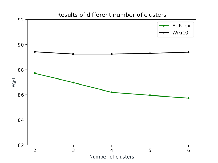
Figure 4: Precision $P@1$ on dataset EURLex and Wiki10, as a function of the number of clusters.

Ablation study. We perform an ablation study to understand the impact of different design choices of APLC based on two datasets, EURLex and Wiki10, with diverse characteristics. Specifically, there are two factors we consider: (1) the impact of the number of clusters, and (2) the impact of the method to partition the label set.

To answer the first question, we assume when the number of clusters is given, the label set is evenly partitioned into each cluster. The other parameters are the same setting as Table 2 and Table 3. We plot Figure 4, precision $P@1$ as a function of the number of clusters $N_{cls}$. Dataset EURLex has the highest $P@1$ 87.72 when $N_{cls}$ is 2. As the value of $N_{cls}$ increases, the precision $P@1$ decreases gradually. When $N_{cls}$ reaches up to 6, the precision $P@1$ is 85.72, with a 2 percent drop. For dataset Wiki10, as the value of $N_{cls}$ increases, the precision $P@1$ decreases slightly. We argue that the large number of clusters tends to harm the performance of the model; however, the degree of impact depends on the characteristics of the dataset.

To answer the second question, we assume the number of clusters $N_{cls}$ is a fixed value, 3. Let $V_{h}$, $V_{1}$ and $V_{2}$ denote the head cluster, the first tail cluster and the second tail cluster, and $P_{h}$, $P_{1}$, $P_{2}$ denote the proportion for which the number of labels in the corresponding cluster accounts. We have three different ways to partition the label set, corresponding three combinations, (0.7,0.2,0.1), (0.33,0.33,0.34) and (0.1,0.2,0.7) for ($P_{h}$, $P_{1}$, $P_{2}$). The other parameters have the same settings as Tables 2 and 3. We plot Figure 5, the prediction precision $P@1$ of different partitions on dataset EURLex and Wiki10. We observe that when more labels are partitioned into the head cluster, the precision $P@1$ is higher on both datasets. This trend is more significant on dataset EURLex, as there is an about 3 percent difference between the first partition and the third partition. However, the impact on dataset Wiki10 is relatively small.

Figure 5: Precision $P@1$ of different partitions on dataset EURLex and Wiki10. Id 1, 2 and 3 denote the partition (0.7, 0.2, 0.1), (0.33, 0.33, 0.34) and (0.1, 0.2, 0.7) respectively.

6 Conclusion

In this paper, we have proposed a novel deep learning approach for the XMTC problem. In terms of prediction accuracy, the performance of our method has achieved new state-of-the-art results over four benchmark datasets, which has shown that the text representation fine-tuned from the pretrained XLNet model is more powerful. Furthermore, we have proposed APLC to deal with extreme labels efficiently. We have carried out theoretical analysis on the model size and computation complexity for APLC. The application of APLC is not limited to XMTC. We believe that APLC may be general enough to be applied to the extreme classification problem as the output layer, especially in tasks where the distributions of classes are unbalanced.

References

- Babbar & Schölkopf (2017) Babbar, R. and Schölkopf, B. Dismec: Distributed sparse machines for extreme multi-label classification. In Proceedings of the Tenth ACM International Conference on Web Search and Data Mining, pp. 721–729. ACM, 2017.
- Bhatia et al. (2015) Bhatia, K., Jain, H., Kar, P., Varma, M., and Jain, P. Sparse local embeddings for extreme multi-label classification. In Advances in Neural Information Processing Systems, pp. 730–738, 2015.
- Chen et al. (2020) Chen, Z., Trabelsi, M., Heflin, J., Xu, Y., and Davison, B. D. Table search using a deep contextualized language model. In Proceedings of the 43rd International ACM SIGIR Conference on Research and Development in Information Retrieval, pp. 589–598. ACM, 2020.
- Conneau & Lample (2019) Conneau, A. and Lample, G. Cross-lingual language model pretraining. In Advances in Neural Information Processing Systems, pp. 7057–7067, 2019.
- Dai et al. (2019) Dai, Z., Yang, Z., Yang, Y., Carbonell, J. G., Le, Q., and Salakhutdinov, R. Transformer-xl: Attentive language models beyond a fixed-length context. In Proceedings of the 57th Annual Meeting of the Association for Computational Linguistics, pp. 2978–2988, 2019.
- Dekel & Shamir (2010) Dekel, O. and Shamir, O. Multiclass-multilabel classification with more classes than examples. In Proceedings of the Thirteenth International Conference on Artificial Intelligence and Statistics, pp. 137–144, 2010.
- Devlin et al. (2019) Devlin, J., Chang, M.-W., Lee, K., and Toutanova, K. Bert: Pre-training of deep bidirectional transformers for language understanding. In Proceedings of the 2019 Conference of the North American Chapter of the Association for Computational Linguistics: Human Language Technologies, volume 1 (Long and Short Papers), pp. 4171–4186, 2019.
- Grave et al. (2017) Grave, E., Joulin, A., Cissé, M., Jégou, H., et al. Efficient softmax approximation for gpus. In Proceedings of the 34th International Conference on Machine Learning-Volume 70, pp. 1302–1310. JMLR.org, 2017.
- Guo et al. (2019) Guo, Q., Qiu, X., Liu, P., Shao, Y., Xue, X., and Zhang, Z. Star-transformer. In Proceedings of the 2019 Conference of the North American Chapter of the Association for Computational Linguistics: Human Language Technologies, Volume 1 (Long and Short Papers), pp. 1315–1325, 2019.
- Howard & Ruder (2018) Howard, J. and Ruder, S. Universal language model fine-tuning for text classification. In Proceedings of the 56th Annual Meeting of the Association for Computational Linguistics (Volume 1: Long Papers), pp. 328–339, 2018.
- Jain et al. (2016) Jain, H., Prabhu, Y., and Varma, M. Extreme multi-label loss functions for recommendation, tagging, ranking & other missing label applications. In Proceedings of the 22nd ACM SIGKDD International Conference on Knowledge Discovery and Data Mining, pp. 935–944. ACM, 2016.
- Jain et al. (2019) Jain, H., Balasubramanian, V., Chunduri, B., and Varma, M. Slice: Scalable linear extreme classifiers trained on 100 million labels for related searches. In Proceedings of the Twelfth ACM International Conference on Web Search and Data Mining, pp. 528–536. ACM, 2019.
- Jasinska et al. (2016) Jasinska, K., Dembczynski, K., Busa-Fekete, R., Pfannschmidt, K., Klerx, T., and Hullermeier, E. Extreme f-measure maximization using sparse probability estimates. In International Conference on Machine Learning, pp. 1435–1444, 2016.
- Joulin et al. (2017) Joulin, A., Grave, É., Bojanowski, P., and Mikolov, T. Bag of tricks for efficient text classification. In Proceedings of the 15th Conference of the European Chapter of the Association for Computational Linguistics: Volume 2, Short Papers, pp. 427–431, 2017.
- Khandagale et al. (2019) Khandagale, S., Xiao, H., and Babbar, R. Bonsai-diverse and shallow trees for extreme multi-label classification. arXiv preprint arXiv:1904.08249, 2019.
- Kim (2014) Kim, Y. Convolutional neural networks for sentence classification. In Proceedings of the 2014 Conference on Empirical Methods in Natural Language Processing (EMNLP), pp. 1746–1751, 2014.
- Kudo & Richardson (2018) Kudo, T. and Richardson, J. Sentencepiece: A simple and language independent subword tokenizer and detokenizer for neural text processing. In Proceedings of the 2018 Conference on Empirical Methods in Natural Language Processing: System Demonstrations, pp. 66–71, 2018.
- Lai et al. (2015) Lai, S., Xu, L., Liu, K., and Zhao, J. Recurrent convolutional neural networks for text classification. In Twenty-ninth AAAI Conference on Artificial Intelligence, 2015.
- Le et al. (2011) Le, H.-S., Oparin, I., Allauzen, A., Gauvain, J.-L., and Yvon, F. Structured output layer neural network language model. In 2011 IEEE International Conference on Acoustics, Speech and Signal Processing (ICASSP), pp. 5524–5527. IEEE, 2011.
- Liu et al. (2017) Liu, J., Chang, W.-C., Wu, Y., and Yang, Y. Deep learning for extreme multi-label text classification. In Proceedings of the 40th International ACM SIGIR Conference on Research and Development in Information Retrieval, pp. 115–124. ACM, 2017.
- Liu et al. (2016) Liu, P., Qiu, X., and Huang, X. Recurrent neural network for text classification with multi-task learning. In Proceedings of the Twenty-Fifth International Joint Conference on Artificial Intelligence, pp. 2873–2879, 2016.
- Mikolov et al. (2011) Mikolov, T., Kombrink, S., Burget, L., Černockỳ, J., and Khudanpur, S. Extensions of recurrent neural network language model. In 2011 IEEE International Conference on Acoustics, Speech and Signal Processing (ICASSP), pp. 5528–5531. IEEE, 2011.
- Mikolov et al. (2013) Mikolov, T., Chen, K., Corrado, G., and Dean, J. Efficient estimation of word representations in vector space. arXiv preprint arXiv:1301.3781, 2013.
- Mnih & Teh (2012) Mnih, A. and Teh, Y. W. A fast and simple algorithm for training neural probabilistic language models. In Proceedings of the 29th International Coference on International Conference on Machine Learning, pp. 419–426, 2012.
- Morin & Bengio (2005) Morin, F. and Bengio, Y. Hierarchical probabilistic neural network language model. In AISTATS, volume 5, pp. 246–252, 2005.
- Prabhu & Varma (2014) Prabhu, Y. and Varma, M. Fastxml: A fast, accurate and stable tree-classifier for extreme multi-label learning. In Proceedings of the 20th ACM SIGKDD international conference on Knowledge discovery and data mining, pp. 263–272. ACM, 2014.
- Prabhu et al. (2018) Prabhu, Y., Kag, A., Harsola, S., Agrawal, R., and Varma, M. Parabel: Partitioned label trees for extreme classification with application to dynamic search advertising. In Proceedings of the 2018 World Wide Web Conference, pp. 993–1002. International World Wide Web Conferences Steering Committee, 2018.
- Radford et al. (2018) Radford, A., Narasimhan, K., Salimans, T., and Sutskever, I. Improving language understanding by generative pre-training, 2018.
- Siblini et al. (2018) Siblini, W., Kuntz, P., and Meyer, F. CRAFTML, an efficient clustering-based random forest for extreme multi-label learning. In Proceedings of the 35th International Conference on Machine Learning, 2018.
- Sun et al. (2019) Sun, C., Qiu, X., Xu, Y., and Huang, X. How to fine-tune bert for text classification? In China National Conference on Chinese Computational Linguistics, pp. 194–206. Springer, 2019.
- Tagami (2017) Tagami, Y. Annexml: Approximate nearest neighbor search for extreme multi-label classification. In Proceedings of the 23rd ACM SIGKDD International Conference on Knowledge Discovery and Data Mining, pp. 455–464. ACM, 2017.
- Vaswani et al. (2013) Vaswani, A., Zhao, Y., Fossum, V., and Chiang, D. Decoding with large-scale neural language models improves translation. In Proceedings of the 2013 Conference on Empirical Methods in Natural Language Processing, pp. 1387–1392, 2013.
- Vaswani et al. (2017) Vaswani, A., Shazeer, N., Parmar, N., Uszkoreit, J., Jones, L., Gomez, A. N., Kaiser, Ł., and Polosukhin, I. Attention is all you need. In Advances in Neural Information Processing Systems, pp. 5998–6008, 2017.
- Wei-Cheng et al. (2019) Wei-Cheng, C., Hsiang-Fu, Y., Kai, Z., Yiming, Y., and Inderjit, D. X-BERT: eXtreme Multi-label Text Classification using Bidirectional Encoder Representations from Transformers. In NeurIPS Science Meets Engineering of Deep Learning Workshop, 2019.
- Wydmuch et al. (2018) Wydmuch, M., Jasinska, K., Kuznetsov, M., Busa-Fekete, R., and Dembczynski, K. A no-regret generalization of hierarchical softmax to extreme multi-label classification. In Advances in Neural Information Processing Systems, pp. 6355–6366, 2018.
- Xu et al. (2019) Xu, H., Liu, B., Shu, L., and Yu, P. Bert post-training for review reading comprehension and aspect-based sentiment analysis. In Proceedings of the 2019 Conference of the North American Chapter of the Association for Computational Linguistics: Human Language Technologies, volume 1, 2019.
- Yang et al. (2019a) Yang, W., Xie, Y., Lin, A., Li, X., Tan, L., Xiong, K., Li, M., and Lin, J. End-to-end open-domain question answering with BERTserini. In NAACL-HLT (Demonstrations), 2019a.
- Yang et al. (2016) Yang, Z., Yang, D., Dyer, C., He, X., Smola, A., and Hovy, E. Hierarchical attention networks for document classification. In Proceedings of the 2016 Conference of the North American Chapter of the Association for Computational Linguistics: Human Language Technologies, pp. 1480–1489, 2016.
- Yang et al. (2019b) Yang, Z., Dai, Z., Yang, Y., Carbonell, J., Salakhutdinov, R. R., and Le, Q. V. Xlnet: Generalized autoregressive pretraining for language understanding. In Advances in Neural Information Processing Systems, pp. 5753–5763, 2019b.
- Yen et al. (2017) Yen, I. E., Huang, X., Dai, W., Ravikumar, P., Dhillon, I., and Xing, E. Ppdsparse: A parallel primal-dual sparse method for extreme classification. In Proceedings of the 23rd ACM SIGKDD International Conference on Knowledge Discovery and Data Mining, pp. 545–553. ACM, 2017.
- Yen et al. (2016) Yen, I. E.-H., Huang, X., Ravikumar, P., Zhong, K., and Dhillon, I. Pd-sparse: A primal and dual sparse approach to extreme multiclass and multilabel classification. In International Conference on Machine Learning, pp. 3069–3077, 2016.
- Yin & Schütze (2018) Yin, W. and Schütze, H. Attentive convolution: Equipping CNNs with RNN-style attention mechanisms. Transactions of the Association for Computational Linguistics, 6:687–702, 2018.
- You et al. (2019) You, R., Zhang, Z., Wang, Z., Dai, S., Mamitsuka, H., and Zhu, S. Attentionxml: Label tree-based attention-aware deep model for high-performance extreme multi-label text classification. In Advances in Neural Information Processing Systems, pp. 5812–5822, 2019.