Anisotropic Diffusion and Traveling Waves of Toxic Proteins in Neurodegenerative Diseases

Abstract

Neurodegenerative diseases are closely associated with the amplification and invasion of toxic proteins. In particular Alzheimer’s disease is characterized by the systematic progression of amyloid-$\beta$ and $\tau$-proteins in the brain. These two protein families are coupled and it is believed that their joint presence greatly enhances the resulting damage. Here, we examine a class of coupled chemical kinetics models of healthy and toxic proteins in two spatial dimensions. The anisotropic diffusion expected to take place within the brain along axonal pathways is factored in the models and produces a filamentary, predominantly one-dimensional transmission. Nevertheless, the potential of the anisotropic models towards generating interactions taking advantage of the two-dimensional landscape is showcased. Finally, a reduction of the models into a simpler family of generalized Fisher-Kolmogorov-Petrovskii-Piskunov (FKPP) type systems is examined. It is seen that the latter captures well the qualitative propagation features, although it may somewhat underestimate the concentrations of the toxic proteins.

1 Introduction

Neurodegenerative disorders are both particularly complex from a scientific and clinical point of view and especially costly from a human and economic perspective. The ongoing effort to address them involves an extensive pipeline of drug development (see, e.g., [1]) with very poor success. It is therefore crucial to enhance our fundamental understanding of the development of such disorders. One of the prevalent viewpoints involves the critical relevance of the formation of protein aggregates, referred to as prion-like aggregates by similarity to prion diseases [2]. In this approach certain proteins develop a toxic variant that can be thought of as seeding the relevant “infection”, progressively leading to an autocatalytic chain reaction of misfolded and aggregated toxic proteins that, in turn, grow and spread throughout the brain inhibiting proper cell function. This type of toxic disruption, unless halted or removed, continues to disrupt progressively the nervous system, ultimately leading to atrophy of different parts of the brain, causing the degradation and eventual death of the patient [3].

An interesting aspect of the prion-like hypothesis is that these proteins are different in different diseases and seeded at different locations, yet there are some universal features of the process and the resulting biomarkers follow similar trends. For example, in Alzheimer’s disease, the relevant proteins have been recognized to be amyloid-$\beta$ (A$\beta$) and $\tau$-protein ($\tau$P). Intriguingly, the two differ significantly in the way they aggregate, their location in the brain and where they originate: the former forms extracellular aggregates and plaques, while the latter operates intra-cellularly, cross-linking microtubules and inducing the formation of large disorganized neurofibrillary tangles [4, 5]. A similar prion-like growth has been argued to be of relevance to the cases of Parkinson’s disease with $\alpha$-synuclein playing a similar role and in amyotrophic lateral sclerosis where the principal biomarker is the TAR DNA binding protein, TDP-43 [6, 7, 8, 9].

Here, we will focus on Alzheimer’s disease (AD) and the associated dynamics of A$\beta$ and $\tau$P. The ubiquitous presence of A$\beta$ plaque in AD patients lead to the so-called “amyloid cascade hypothesis” of Hardy and collaborators [10, 11], which has contributed significantly to the research directions of the relevant field for over 25 years [12]. Indeed, at the present stage of drug development [1], about half of the current efforts towards disease-modifying therapies, and about 32% of the total of currently tested drugs, are primarily focused on A$\beta$ and are classified as “anti-amyloid” drugs. Also, another 4% of currently tested drugs are “anti-$\tau$” and yet another 4% are both anti-amyloid and anti-$\tau$. In total, a remarkable 40% of all currently developed drugs focus exclusively on A$\beta$ and $\tau$P, while only 21% focus on other disease-modifying factors. For reference, another 28% of potential drugs targets neuropsychiatric symptoms, while 11% focuses on cognitive enhancers.

These efforts have also motivated attempts to model the progression of A$\beta$ and $\tau$P toxicity [13, 14, 15] in line with corresponding measurements of such biomarkers from different types of scans [16]. Indeed, recent efforts have shown that at least some of the clinical antibodies under consideration, such as aducanumab, may hold promise towards binding with fibrillar forms of A$\beta$, reducing the flux of its oligomeric forms and ultimately yield positive outcomes in clinical trials [17].

Our aim in the present work is to present some simplifying models of the coupled dynamics of A$\beta$ and $\tau$P in the spirit of [13, 14, 15], but focusing predominantly in two spatial dimensions as it has been shown to capture most of the qualitative dynamics for the progression of a single toxic protein [14]. Our spatial-temporal model is originally based on chemical kinetics in line with the recent efforts of [14, 15], rather than starting from a purely phenomenological Fisher-KPP (FKPP for short, named after the ubiquituous Fisher-Kolmogorov-Petrovskii-Piskunov model) [18], as e.g., in [13]. It incorporates 4 populations, namely healthy and toxic variants of the A$\beta$ and $\tau$P. In addition to the generation of the healthy proteins and the decay of both healthy and toxic ones with corresponding rates, the conversion of healthy A$\beta$ and $\tau$P into respective toxic variants is accounted for and so is the role of toxic A$\beta$ towards catalyzing the production of toxic $\tau$P [14, 15]. We observe different scenarios of so-called primary tauopathies (where each toxic species can exist on its own and they can also co-exist) and so-called secondary tauopathies, where the existence of toxic $\tau$P is contingent upon the presence of toxic A$\beta$. We examine each scenario in a quasi-1d setting where the role of the second dimension is simply in providing a weak lateral spreading of the waves. We also examine a genuinely 2d scenario, where the transverse interaction of the toxic waves is critical for the spreading of the disorder, as a way of illustrating the effect of dimensionality. Finally, we illustrate how to approximate the model by an effective (generalized) FKPP variant and compare the latter with the full results finding very good qualitative agreement despite the partial quantitative disparities between the two.

Our presentation is structured as follows. In section II, we discuss the models at the different levels of description (chemical kinetic 4-component model and its two-component FKPP reduction) and some of their salient features. Then, in section III, we will present the different simulations for primary and secondary tauopathies, without and with incorporating a significant role of the transverse degrees of freedom. The comparison to the FKPP will also be given to obtain a sense of the relevance of studying the less computationally expensive models of the latter type. Finally, in section IV, we will summarize our findings and present our conclusions.

2 Model Formulation

Our principal model, presented in [15], features four species: healthy A$\beta$ and $\tau$P and toxic A$\beta$ and $\tau$P. Here are the processes involved in each species:

• Healthy A$\beta$ diffuses anisotropically over the flat domain. It is produced with a constant rate $a_{0}$ and is cleared with a clearance rate $a_{1}$. Moreover, the interaction of healthy and toxic A$\beta$ results in the toxification of healthy A$\beta$ proteins. The healthy A$\beta$ concentration is denoted as $u(x,y,t)$, with the independent variables being $(x,y)$ in space and $t$ for time.

• In a similar vein, toxic A$\beta$ proteins diffuse with similar diffusivities anisotropically over our two-dimensional slice. They are cleared with a rate $\tilde{a}_{1}$ and get produced by the toxification of the corresponding healthy concentration. With tildes being used for the toxic species, the relevant population is denoted by $\tilde{u}(x,y,t)$.

• Similarly, the healthy $\tau$P concentration is denoted by $v(x,y,t)$ and involves diffusion, production at a constant rate $b_{0}$ and clearance with a clearance rate $b_{1}$. Here, toxic $\tau$P are produced either by direct interaction of healthy and toxic $\tau$P with rate $b_{2}$ or catalyzed by the (surrounding) presence of toxic A$\beta$ with rate $b_{3}$.

• Finally, similar anisotropic diffusion properties are posited also for toxic $\tau$P, with a clearance rate $\tilde{b}_{1}$ and production by the two above mechanisms of toxification of the healthy $\tau$P population.

Mathematically translating the above 4 populations and the respective assumptions, we obtain the following nonlinear partial differential equations:

$$u_{t} = D_{x}\left(u_{xx}+\epsilon u_{yy}\right)+a_{0}-a_{1}u-a_{2}u\tilde{u},$$ (1)

$$\tilde{u}_{t} = D_{x}\left(\tilde{u}_{xx}+\epsilon\tilde{u}_{yy}\right)-\tilde{a}_{1}\tilde{u}+a_{2}u\tilde{u},$$ (2)

$$v_{t} = D_{x}\left(v_{xx}+\epsilon v_{yy}\right)+b_{0}-b_{1}v-b_{2}v\tilde{v}-b_{3}v\tilde{u}\tilde{v},$$ (3)

$$\tilde{v}_{t} = D_{x}\left(\tilde{v}_{xx}+\epsilon\tilde{v}_{yy}\right)-\tilde{b}_{1}\tilde{v}+b_{2}v\tilde{v}+b_{3}v\tilde{u}\tilde{v}.$$ (4)

Here, for simplicity we have assumed that all the diffusivities are equal and are assigned to be $D_{x}$ along the $x$-axis, while they are $D_{y}=\epsilon D_{x}$ along the $y$-axis. All parameters and variables are assumed to be positive. Finally, the subscripts denote partial derivatives with respect to the corresponding independent variables.

Following also the considerations of [15], one defines a “damage” variable $q(x,y,t)$ based on the following (trivial in space) PDE:

$$q_{t}=\left(k_{1}\tilde{u}+k_{2}\tilde{v}+k_{3}\tilde{u}\tilde{v}\right)(1-q).$$ (5)

This naturally tends to a stable fixed point of $q(x,y,t)=1$ (maximal damage), starting from an initial condition of no-damage, i.e., $q(x,y,0)=0$.

A relevant consideration is that of identifying the fixed points in this model. There are, generally speaking, 4 equilibrium fixed points in this case.

1. $(\frac{a_{0}}{a_{1}},0,\frac{b_{0}}{b_{1}},0)$ is the always unstable (in the realm of this model) healthy state. The assumption here is that we are modeling an early stage of the emergence of the neurodegenerative disorder.

2. $(\frac{\tilde{a}_{1}}{a_{2}},\frac{a_{0}}{\tilde{a}_{1}}-\frac{a_{1}}{a_{2}},\frac{b_{0}}{b_{1}},0)$ is a state devoid of toxic $\tau$P, but bearing toxic A$\beta$. For this state to be biologically meaningful (i.e., reflecting positive concentrations), the assumption is $a_{0}a_{2}>a_{1}\tilde{a}_{1}$.

3. Similarly, $(\frac{a_{0}}{a_{1}},0,\frac{\tilde{b}_{1}}{b_{2}},\frac{b_{0}}{\tilde{b}_{1}}-\frac{b_{1}}{b_{2}})$ is a state with only healthy A$\beta$, but bearing both healthy and toxic $\tau$P. Here, biological relevance dictates that $b_{0}b_{2}>b_{1}\tilde{b}_{1}$.

4. Lastly, there exists a homogeneous state with all four populations, healthy and toxic ones alike, being non-vanishing, whereby $u=\tilde{a}_{1}/a_{2}$, $\tilde{u}=\frac{a_{0}}{\tilde{a}_{1}}-\frac{a_{1}}{a_{2}}$, $v=\frac{\tilde{a}_{1}a_{2}\tilde{b}_{1}}{P}$ and $\tilde{v}=\frac{b_{0}}{\tilde{b}_{1}}-\frac{\tilde{a}_{1}a_{2}b_{1}}{P}$, where $P=\tilde{a}_{1}a_{2}b_{2}-a_{1}\tilde{a}_{1}b_{3}+a_{0}a_{2}b_{3}$. For all 4 equilibria to be present, it is necessary that both inequality constraints are satisfied enabling the previous two equilibria to exist. Interestingly, in this setting, the concentration of the toxic A$\beta$ (at equilibrium) remains the same as for the equilibrium devoid of toxic $\tau$P, yet the concentration of toxic $\tau$P is higher than that in which the only toxic species is $\tau$P. This property is a consequence of the one-way coupling (A$\beta$ influences the production of $\tau$P but $\tau$P does not influence A$\beta$, as observed experimentally).

The above observation leads to a classification of the so-called tauopathies. By this, we will mean scenarios involving toxic contributions from both A$\beta$ and $\tau$P. In the case of a primary tauopathy, both of the above inequalities are satisfied, then all 4 equilibria will exist. For a secondary tauopathy, we have $a_{0}a_{2}>a_{1}\tilde{a}_{1}$, while $b_{0}b_{2}<b_{1}\tilde{b}_{1}$, it is still possible to have an equilibrium where both toxic components are concurrently present, yet $\tau$P cannot be toxic by itself (i.e., in the absence of toxic A$\beta$). Naturally for this scenario of secondary tauopathy to occur, the relevant coefficient $b_{3}$ should be sufficiently large. We will examine both of these scenarios in what follows.

Lastly, we consider the reduction of the model into a pair of FKPP-type PDEs for the toxic components alone. To do so, an effective assumption of sufficiently larger (than the toxic) healthy concentrations of the two proteins is relevant to incorporate. In particular, assuming an effectively space- and time-independent concentration of healthy A$\beta$ yields $u=a_{0}/(a_{1}+a_{2}\tilde{u})$. This, in turn, under these assumptions of $\tilde{u}\ll u$ can be approximated by $u\approx\frac{a_{0}}{a_{1}}(1-\frac{a_{2}}{a_{1}}\tilde{u})$. In a similar vein, we can extract, via leading order Taylor expansion, $v=\frac{b_{0}}{b_{1}}(1-\frac{b_{2}}{b_{1}}\tilde{v}-\frac{b_{3}}{b_{1}}\tilde{u}\tilde{v})$. Then, the resulting generalized FKPP equations stemming from the substitution of these approximations into Eqs. (2) and (4) are:

$$\tilde{u}_{t} = D_{x}\left(\tilde{u}_{xx}+\epsilon\tilde{u}_{yy}\right)+\left(\frac{a_{2}a_{0}}{a_{1}}-\tilde{a}_{1}\right)\tilde{u}-\frac{a_{2}^{2}a_{0}}{a_{1}^{2}}\tilde{u}^{2},$$ (6)

$$\tilde{v}_{t} = D_{x}\left(\tilde{v}_{xx}+\epsilon\tilde{v}_{yy}\right)+\left(\frac{b_{2}b_{0}}{b_{1}}-\tilde{b}_{1}+\frac{b_{3}b_{0}}{b_{1}}\tilde{u}\right)\tilde{v}-\left(\frac{b_{2}^{2}b_{0}}{b_{1}^{2}}+\frac{2b_{2}b_{3}b_{0}}{b_{1}^{2}}\tilde{u}+\frac{b_{3}b_{0}}{b_{1}^{2}}\right)\tilde{v}^{2}.$$ (7)

We will also explore the results of the system of Eqs. (6)-(7) and compare it with the observations stemming from Eqs. (1)-(4), as concerns the evolution of both primary and secondary tauopathies in what follows. Linearized theory predicts the speeds of propagation of the corresponding resulting fronts, namely for the front interpolating between states $1$ and $2$, we have:

$$c^{12}=2\sqrt{D_{x}\left(\frac{a_{2}a_{0}}{a_{1}}-\tilde{a}_{1}\right)}.$$ (8)

We consider here the speed of propagation along the dominant direction of diffusion, namely the x-axis, since we will assume $\epsilon\ll 1$ in what follows. On the other hand, for the front interpolating between the homogeneous states $1$ and $3$, we will have, respectively:

$$c^{13}=2\sqrt{D_{x}\left(\frac{b_{2}b_{0}}{b_{1}}-\tilde{b}_{1}\right)}.$$ (9)

Once the right propagating wave of the left blob and the left one of the right blob reach each other and interact, they will achieve a state of co-existence and the resulting propagation speed that is obtained via linearization around the co-existence state is:

$$c^{24}=2\sqrt{\frac{\tilde{\rho}_{2}}{a_{2}b_{1}\tilde{a}_{1}}}\sqrt{\tilde{a}_{1}\left(a_{2}\left(b_{0}b_{2}-b_{1}\tilde{b}_{1}\right)-a_{1}b_{0}b_{3}\right)+a_{0}a_{2}b_{0}b_{3}}.$$ (10)

Having set up the relevant models, we now turn to the corresponding numerical results.

3 Numerical Results

3.1 Primary Tauopathy

We start our exposition of the numerical results by examining a setting of primary tauopathy (i.e., where all 4 relevant uniform equilibrium states exist). In this setting the 2nd state (involving no toxic $\tau$P) and the 3rd state (involving no toxic A$\beta$) are only attracting in the absence of one of the toxic species. When both toxic species are present, the situation favors the co-existing state where both toxic species are present (i.e., the 4th one). Hence, we design the following numerical experiment: on the one side, we seed a narrow blob of toxic A$\beta$, while on the other side, we seed a similar blob but of toxic $\tau$P, so as to see how the respective toxicities will interact upon their propagation. In this primary tauopathy, we select $a_{0}=b_{0}=a_{1}=a_{2}=b_{1}=b_{2}=1$, while $\tilde{a}_{1}=\tilde{b}_{1}=3/4$ and $b_{3}=1/2$. The initial conditions associated with this numerical experiment shown in Fig. 1 involve uniform profiles $u(x,y,0)=1$, $v(x,y,0)=1$ for healthy A$\beta$ and $\tau$P, while for the toxic proteins we assume a small blob of initial concentrations in the form:

$$\tilde{u}(x,y,0) = \frac{1}{3}{\rm sech}^{2}\left((x+20)^{2}+10y^{2}\right),$$ (11)

$$\tilde{v}(x,y,0) = \frac{1}{3}{\rm sech}^{2}\left((x-20)^{2}+10y^{2}\right).$$ (12)

Notice that the relevant results have been found to be generic within their corresponding regimes of parametric inequalities, hence the particular value of the parameters, as well as the amplitude and precise shape of the initial condition blobs do not play a crucial role as regards the phenomenology reported below.

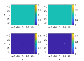
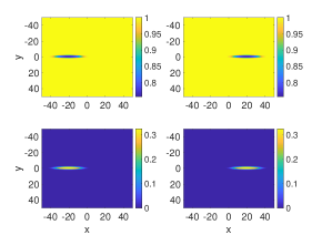
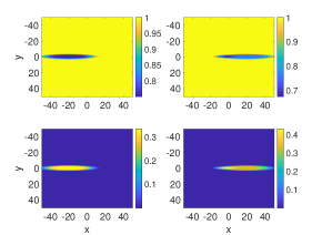
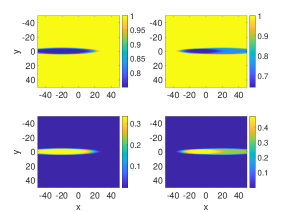
Figure 1: Numerical evolution snapshots of a primary tauopathy via 4 $2\times 2$ sets of 4 panels each. The first set of panels is at $t=0.5$, the second at $t=30$, the third at $t=50$ and the last at $t=70$. What is shown is a contour plot of the spatial distribution of all four of the relevant field concentrations: the healthy A$\beta$ (top left), the healthy $\tau$P (top right), the toxic A$\beta$ (bottom left) and the toxic $\tau$P (bottom right).

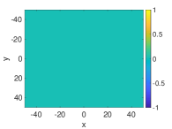
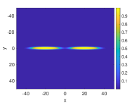
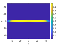
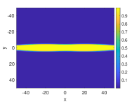
Figure 2: Evolution of the damage function $q(x,y,t)$ at the same times as for the above simulation. I.e., $t=0.5$ at the top left, $t=30$ at the top right, $t=50$ at the bottom left and $t=70$ at the bottom right. It can be clearly seen how the evolving initial spots expand into a “corridor” of damage over the dynamical evolution.

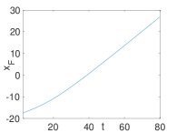
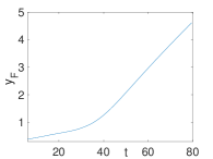
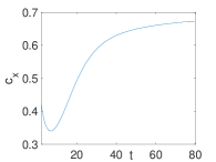
Figure 3: The left panel shows the x-position of the center of the front ($x_{F}$) that starts on the left (and moves towards the right) within the numerical experiment of a primary tauopathy. The middle panel shows the corresponding y-position $y_{F}$ The speed $c_{x}$ along the x-axis can be clearly seen in the right panel to approach the asymptotic value of $c_{x}=2^{-1/2}$. Correspondingly the $y$-speed (not shown here) can be seen to approach the limiting value $c_{y}=(2\epsilon)^{-1/2}$.

It can be observed that the scenario described theoretically is realized here: the symmetry of the coefficients leads to an equally rapid propagation of the two (left and right) blobs in both directions with a speed of $\sqrt{1/2}$. Indeed, we can observe the damage function evolving accordingly and symmetrically expanding the disorder across the domain in Fig. 2. More concretely, Fig. 3 captures one of these fronts as they start on the left side of the domain and propagate rightward along the $x$-direction (left panel), while they also expand along the $y$-direction (middle panel). Indeed, here, the simulation involves a factor of $\epsilon=0.01$, leading to a tenfold reduction of the corresponding speed along the $y$-direction. It can be seen that our numerical evaluation of the associated speed, after a transient (which can also be observed in the left and middle panels), settles in the vicinity of its anticipated asymptotic value (right panel of Fig. 3). Importantly, also, however, we observe in Fig. 1 the formation of the co-existing (4th) state of the two toxic proteins A$\beta$ and $\tau$P as the prevalent state where the two populations overlap. This can be especially discerned in the bottom left and bottom right panels of the figure where the higher concentration of the toxic $\tau$P clearly illustrates the relevant state (recall that the A$\beta$ does not modify its equilibrium concentration in the presence of $\tau$P). Notice also that the damage function, as defined herein, also does not appear to feature an immediately discernible signature of the co-existence state, as per Fig. 2.

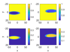
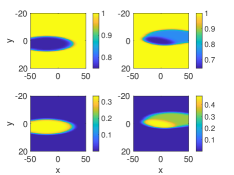
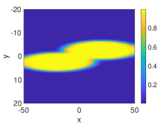
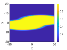
Figure 4: Similar to the results of the primary tauopathy case, but now in a case where the geometry/two-dimensionality of the initial configuration matters more: initially the waves of toxicity of A$\beta$ and $\tau$P are offset as per Eqs. (13) and (14). The four fields are shown for $t=60$ (top left $2\times 2$ panels) and $t=80$ (top right $2\times 2$ panels) along with their corresponding damage variable spatio-temporal spread (bottom panels).

To explore the effects of geometry and two-dimensionality of the system, we now turn to the consideration of a scenario where the initial toxicity of the A$\beta$ and $\tau$P are not “aligned”. In this case, while we retain the initially uniform profile in the healthy populations of the relevant biomarkers, we offset vertically the corresponding toxic initial populations as follows:

$$\tilde{u}(x,y,0) = \frac{1}{3}{\rm sech}^{2}\left((x+20)^{2}+5(y-2.5)^{2}\right)$$ (13)

$$\tilde{v}(x,y,0) = \frac{1}{3}{\rm sech}^{2}\left((x-20)^{2}+5(y+2.5)^{2}\right)$$ (14)

In this case too, during the early stages, the propagation of the neurodegenerative waves (the one connecting the 1st and the 2nd homogeneous state on the left and the one connecting the 1st and the 3rd such on the right) occurs principally along quasi-one-dimensional “corridors” within the system. As can be seen in Fig. 4, however, at later times, as these waves spread in the lateral direction, they interact and form an “oblique” front. Here, the co-existent state of toxicity of the two species dominates, leading to an expansion of the relevant front in both directions. This oblique interaction pattern also affects the spread of the corresponding damage function as can be observed in the bottom panels of the figure. Once again, the latter bears no discernible features of the toxic co-existence associated with the 4th equilibrium state (in comparison to the 2nd or 3rd one). Still, the expanding front of co-existent toxicity is especially evident in the right column of the snapshots shown (and even more so in the movies of [19]).

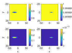
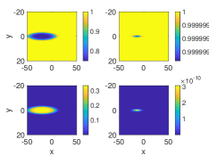
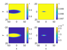
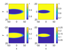
Figure 5: Similar to the results of the primary tauopathy case, but now in the scenario of a secondary tauopathy and for $t=25$, $50$, $75$ and $100$. Notice how the toxic $\tau$P is absent early on, yet it emerges as a result of its overlap with toxic A$\beta$ and subsequently grows in a rapidly expanding front.

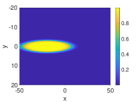
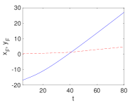
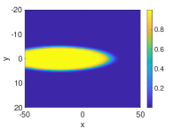
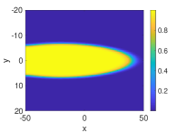
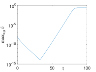
Figure 6: The left set of panels involves the damage function at the same times as above. The top right panel shows the expansion of the right-moving toxic front of A$\beta$ in the x (solid) and y (dashed) axis via its center position $(x_{F},y_{F})$. The secondary nature of the tauopathy is evident in the bottom right showing how the toxic $\tau$P decays until it overlaps with the rightward propagating toxic A$\beta$ leading to its rapid growth and eventual saturation in the co-existing toxic state.

3.2 Secondary Tauopathy

We now turn to a scenario of secondary tauopathy for which the presence of toxic A$\beta$ is required for toxic $\tau$P. As discussed in the theory, we select a sufficiently large value of $b_{3}=3$, and keep all other coefficients the same except for $\tilde{b}_{1}=4/3$, so that the third equilibrium (of solely toxic $\tau$P) is absent. In this case, in terms of initial conditions, the first three components are similar to our original numerical experiment involving uniform populations for the healthy biomarkers and a toxic A$\beta$ population given by Eq. (11). However, here the toxic component of the $\tau$P is given by:

$$\tilde{v}(x,y,0) = 10^{-8}{\rm sech}^{2}\left((x-20)^{2}+10y^{2}\right).$$ (15)

In this case, a fundamentally different dynamical evolution of the disorder can be observed. Indeed, the initial stages of the simulation illustrate a decrease of the toxic levels of $\tau$P (cf. the early times in Fig. 5 and also the bottom right panel of Fig. 6, reporting the maximal concentration thereof). However, over time, the expansion of the front involving the toxic A$\beta$ eventually leads to an overlap with the toxic $\tau$P that, in turn, ignites the nucleation and expansion of the 4th homogeneous state, the one of co-existent toxicity of the two proteins. The relevant “droplet” (of $\tau$P) can be seen to rapidly expand and eventually catch up to the front of expanding toxic A$\beta$; see the left and right panels of Fig. 5. While this evolution is not immediately evident in the damage spatio-temporal evolution panels of Fig. 6, it is clear in the growth and eventual saturation of the toxic $\tau$P maximal concentration (bottom right panel of Fig. 6), as well as in the movies of [19]. Notice that we also considered scenarios of non-collinear propagation in this secondary tauopathy as well (not shown here). The main difference there was that the non-collinear propagation delayed the occurrence of overlap between the very weak toxic $\tau$P pulse and the propagating toxic A$\beta$ front, thus considerably delaying the emergence and expansion of the 4th homogeneous state of co-existing toxicity.

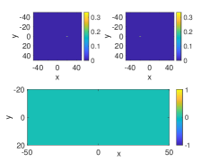
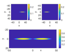
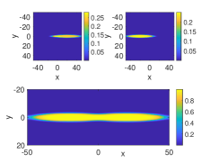
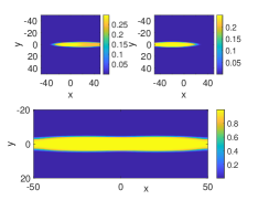
Figure 7: Similar to the results of the primary tauopathy case (Figs. 1 and 2), but now in the scenario of collinear propagation within a two-species FKPP-type model only for the toxic components of A$\beta$ and $\tau$P. Each triplet shows the two toxic components, as well as the damage variable $q$ at the same times as before.

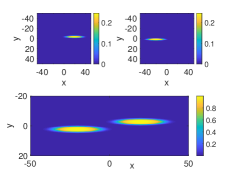
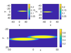
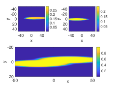
Figure 8: Similar to the results of the primary tauopathy case in the non-collinear case of Fig. 4, but now in the scenario of a two-species model only for the toxic components of A$\beta$ and $\tau$P. Again only the two toxic components and the damage variable are shown in each triplet of panels.

3.3 Reduction to FKPP

Finally, we considered the examples of primary tauopathy in the context of the FKPP-type models of Eqs. (6)-(7), both in the realm of the collinear propagation of the two invasion fronts (the toxic A$\beta$ and the toxic $\tau$P) in Fig. 7, as well as in that of the oblique interaction in Fig. 8. It is important to observe that in both cases the qualitative dynamics are in close analogy to the full evolution of both the healthy and toxic populations in Figs. 1 and 4, respectively. Notice that in the FKPP case, we only show the two toxic species spatial concentration contour plots at different snapshots in time, along with the corresponding damage contour profiles. It can be clearly seen that the qualitative correspondence persists over the time scales shown. Nevertheless at the quantitative level, we see that the assumption of a much higher healthy concentration is progressively less adequate. This eventually leads to an underestimation of the toxic concentration of the associated proteins. Nevertheless, the effective simplification at the level of the FKPP equations is well suited towards understanding the associated phenomenology in all the cases that we have examined.

4 Conclusions

In the present work, we have explored the evolution of toxic fronts of proteins such as amyloid-$\beta$ and the $\tau$-protein within a two-dimensional terrain, i.e., the propagation of neurodegenerative waves within a two-dimensional slice. Our formulation was based on chemical kinetics, following earlier works such as [14, 15] and considering both healthy and toxic populations of the relevant proteins and the spatio-temporal evolution of their concentrations. It was assumed that the healthy proteins are produced and degraded at a given rate, and there is a conversion of the healthy proteins into toxic ones upon interaction with a toxic “seed”. In the case of $\tau$P, this is further catalyzed by the presence of toxic A$\beta$. In this setting, four equilibrium fixed points were identified and the heteroclinic orbits connecting them dominated the relevant dynamics. The conditions were identified under which (parametrically) the different fixed points exist and when all were present, their interaction was considered primarily in two scenarios. The first, characterized as a primary tauopathy involved the presence of all four fixed points (toxic fronts of A$\beta$ and $\tau$P could exist independently, but also interact to form a toxic co-existence front). The second one, referred to as secondary tauopathy featured no toxic $\tau$P alone, but only in conjunction with toxic A$\beta$. It was also observed how the two-dimensional geometry and the anisotropic diffusion can conspire to enable these fronts to propagate along quasi-1d corridors, but concurrently can allow the interaction of the propagating fronts to produce an oblique wave of toxic co-existence between the different proteins. Finally, a reduced model solely featuring the toxic components was developed and it was shown that it quite adequately represents the examples considered qualitatively, although, naturally, some of the quantitative aspects are suitably modified.

It is particularly relevant to consider this class of models further, both from the perspective of biological “adequacy” (and the potential inclusion of suitable further biologically relevant traits) and faithfulness and, if relevant, from the perspective of mathematical control and optimization. More concretely, here these models have been illustrated from the point of view of two-dimensional partial differential equations. However, suitable connectivity networks exist within the brain and have been mapped [13, 14]. Incorporating the associated connectivity (i.e., the adjacency matrices thereof) allows to track relevant dynamics on a more realistic network. This is of particular interest presently in the context of neurodegenerative diseases; see for a recent example of experimental observations and associated linear modeling for Parkinson’s disease the work of [20]. On the other hand, it is clear that the model used here is an initial effort to represent the spreading of disorder when the organism is “on the verge” of disease. However, it is relevant to develop a variant of this model that may feature physiological function but may be able (upon a suitable “bifurcation event”) to turn to the preferentiality for disease dynamics. A related question is that of attempting to connect parameters postulated herein with realistic numbers stemming from biological experiments. Estimating production and clearance levels of these proteins may be within reach based on recent experimental biomarker tracking capabilities [16]. Other coefficients, such as those of toxic conversion of the proteins may be more difficult to assess but the present model (and its distinction between different types of tauopathies) suggests the relevance of consideration of such experiments.

Lastly, should such a model be possible to establish on a more firm biological basis (rather than a more phenomenological one as is done here), the benefits would be significant at various levels. One could consider how to inhibit the propagation of the fronts examined herein and what this would require from a biological intervention (drug administration) perspective. A controlled propagation, a slowing down and ideally a halting of such toxic fronts would be an intriguing target for control theory objectives applied to such infinite dimensional models. Enabling such a mathematical testing framework would be of particular relevance and interest, even though recent advances (such as those of [17]) suggest that this may need to be done at a more sophisticated level, like for example that of considering distributions of the relevant proteins. This stems from the emerging necessity to reduce the flux of oligomeric (but not monomeric) forms of, e.g., A$\beta$ in order to achieve cognitive improvement in some of the most recent experimental studies [17].

Ackowledgments. The support for A.G. by the Engineering and Physical Sciences Research Council of Great Britain under research grant EP/R020205/1 is gratefully acknowledged. This material is based upon work supported by the US National Science Foundation under Grant DMS-1809074 (P.G.K.). P.G.K. also acknowledges support from the Leverhulme Trust via a Visiting Fellowship and thanks the Mathematical Institute of the University of Oxford for its hospitality during this work.

References

- [1] J. Cummings, G. Lee, A. Ritter, M. Sabbagh, K. Zhong, Alzheimer & Dementia: Translational Research & Clinical Interventions 5, 272 (2019).
- [2] M. Jucker and L.C. Walker, Nature (London) 501, 45 (2013).
- [3] J. Brettschneider, K. Del Tredici, V.M.-Y. Lee, J.Q. Trojanowski, Nat. Rev. Neurosci. 16, 109 (2015).
- [4] L.C. Walker and M. Jucker, Annu. Rev. Neurosci. 38, 87 (2015).
- [5] M. Goedert, M. Masuda-Suzukake, B. Falcon, Brain 140, 266 (2017).
- [6] I.R.A. Mackenzie, R. Rademakers, Curr. Opin. Neurol. 21, 693 (2008).
- [7] L. Stefanis, Cold Spring Harb. Perspect. Med. 2, a009399 (2012).
- [8] M. Cruz-Haces, J. Tang, G. Acosta, J. Fernandez, R. Shi, Transl. Neurodegener. 6, 20 (2017).
- [9] J.C. Watts, C. Condello, J. Stöhr, A. Oehler, J. Lee, S.K. DeArmond, L. Lannfelt, M. Ingelsson, K. Giles, S.B. Prusiner, Proc. Natl. Acad. Sci. USA 111, 10323 (2014).
- [10] J. Hardy. D. Allsop, Trends Pharmacol. Sci. 12, 383 (1991).
- [11] J.A. Hardy, G.A. Higgins, Science 256, 184 (1992).
- [12] D. Selkoe, J.A. Hardy, EMBO Mol. Med. 8, 595 (2016).
- [13] J. Weickenmeier, E. Kuhl, A. Goriely, Phys. Rev. Lett. 121, 158101 (2018).
- [14] J. Weickenmeier, M. Jucker, A. Goriely, E. Kuhl, J. Mech. Phys. Solids 124, 264 (2019).
- [15] T. Thompson, E. Kuhl, and A. Goriely, Protein-protein interactions in neurodegenerative diseases: a conspiracy theory, preprint (2020). doi.org/10.1101/2020.02.10.942219
- [16] R.J. Bateman et al., N Engl J Med. 367, 795 (2012).
- [17] S. Linse, T. Scheidt, K. Bernfur, M. Vendruscolo, C.M. Dobson, S.I.A. Cohen, E. Sileikis, M. Lundquist, F. Qian, T. O’Malley, T. Bussiere, P.H. Weinreb, C.K. Xu, G. Meisl, S. Devenish, T.P.J. Knowles, O. Hannson, bioRxiv, https://doi.org/10.1101/815308
- [18] J.D. Murray, Mathematical Biology Springer-Verlag (New York, 1989).
- [19] Movies for the evolution of the different species and the damage function of each of the scenarios shown here are illustrated in: https://www.dropbox.com/sh/w07164jndgchi3a/AACTb-BX6oVwFBu2Pn7E25t0a?dl=0
- [20] M.X. Henderson et al. Nat. Neurosci. 22, 1248 (2019).