Abstract

Study populations are typically sampled from limited points in space and time, and marginalized groups are underrepresented. To assess the external validity of randomized and observational studies, we propose and evaluate the worst-case treatment effect (WTE) across all subpopulations of a given size, which guarantees positive findings remain valid over subpopulations. We develop a semiparametrically efficient estimator for the WTE that analyzes the external validity of the augmented inverse propensity weighted estimator for the average treatment effect. Our cross-fitting procedure leverages flexible nonparametric and machine learning-based estimates of nuisance parameters and is a regular root-$n$ estimator even when nuisance estimates converge more slowly. On real examples where external validity is of core concern, our proposed framework guards against brittle findings that are invalidated by unanticipated population shifts.

1 Introduction

When the study population is different from those affected by the treatment, the external validity of a study’s finding may be called into question. Study populations are often sampled from a particular set of points in space and time and may not represent future populations of interest [17, 57, 67, 31]. Furthermore, study populations often lack diversity, and minority groups are underrepresented. For example, out of $10,000+$ cancer clinical trials funded by the National Cancer Institute, less than 5% of participants were non-white [19, 73]. When the treatment effect is heterogeneous, both randomized and observational studies lose external validity outside the study population. While large-scale randomized trials offer a “gold standard” for internal validity, their external validity can be nevertheless called into question over spatiotemporal changes in the population [30, 12].

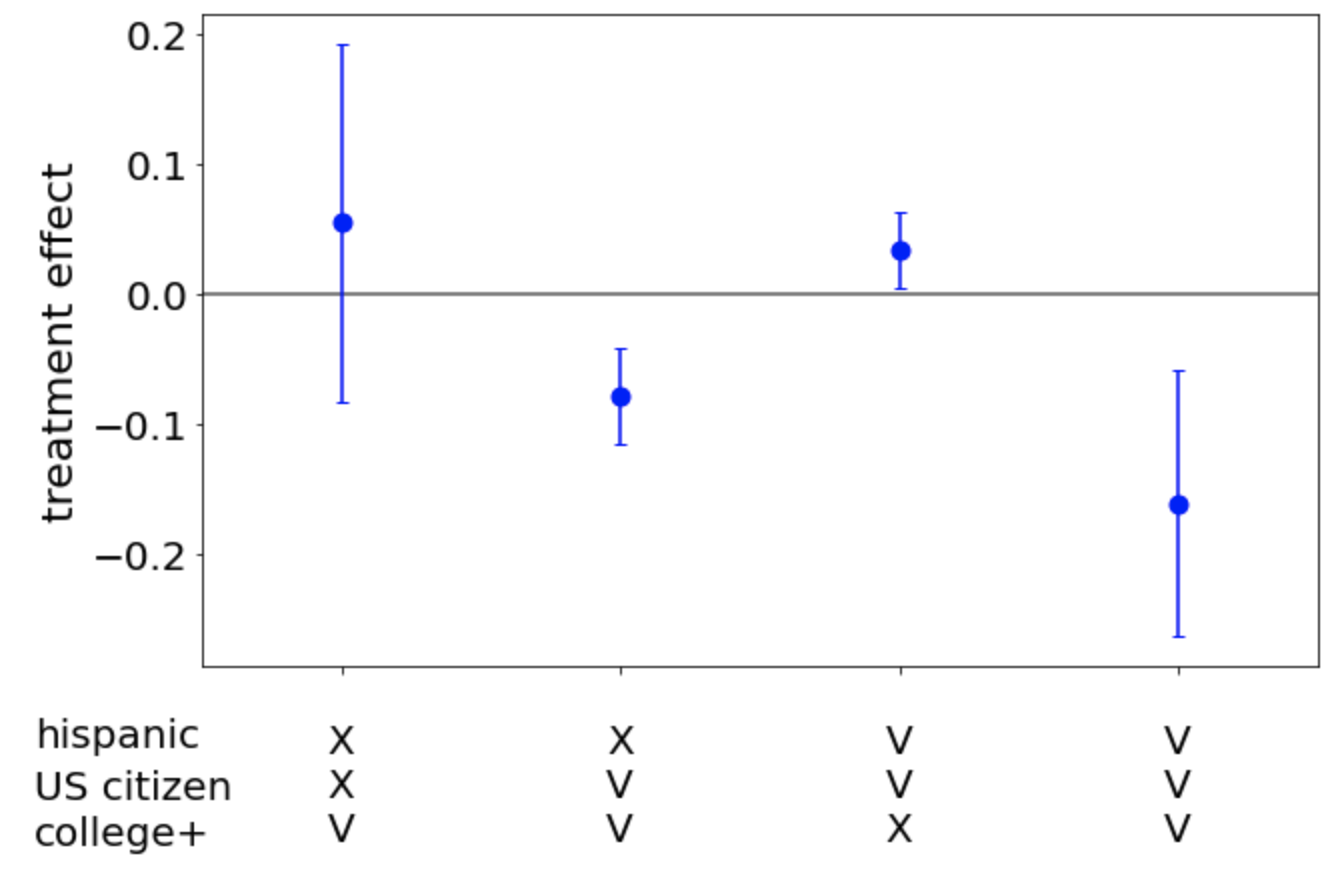
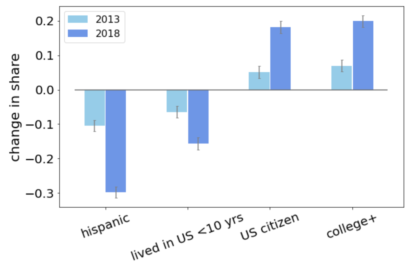
(a) Intersectionality of treatment effects (2009)	(b) Change in shares from 2009 to 2013 & 2018

Figure 1: Effect of Medicaid enrollment on doctors’ visit for low-income adults (NHIS)

Existing approaches for assessing external validity require the knowledge of the target population [44, 2, 24, 74, 76, 54, 1, 58]. However, target populations chosen at the time of analysis may not be sufficient to guarantee external validity over unforeseen shifts in the population that occur post-analysis. Heuristic approaches such as estimating treatment effects over fixed subgroups are similarly limited as effects typically vary over a combination of multiple characteristics like race, gender, age, and income, a phenomenon we refer to as intersectionality.

To illustrate these challenges, consider estimating the effect of Medicaid enrollment on doctors’ office utilization based on the National Health Interview Survey (NHIS) in 2009, where we focus on whether the individual made any visits to doctors two weeks prior to the survey date as the main outcome. Observed treatment effects and resulting decisions in 2009 must remain valid over a priori unknown shifts in the population over time. We observe substantial intersectionality in the treatment effect (Figure 1a): for Hispanic U.S. citizens, the treatment effect changes signs depending on professional degree attainment. In the decade following 2009 (“future”), there is a major shift in the underlying population (Figure 1b), and observed effects in 2009 are no longer valid in the future, as we later illustrate in Section 3.

To assess external validity over unanticipated population shifts in the population, we propose and study the worst-case treatment effect, $\mbox{WTE}_{\alpha}$, defined over all subpopulations that comprise at least $\alpha$-fraction of the study population (see Eq. (2) to come). As the $\mbox{WTE}_{\alpha}$ bounds the average treatment effect (ATE) and reduces to it when $\alpha=100\%$, the WTE analyzes the sensitivity of an average-case finding under population shifts, guaranteeing that conservative findings using the WTE remain valid uniformly over subpopulations. For example, if low-income Hispanic U.S. citizens with professional degrees comprise at least $20\%$ of the study population, positive findings with respect to $\mbox{\rm WTE}_{.2}$ guarantee the treatment remains effective over this subgroup.

We develop a semiparametrically efficient estimator of $\mbox{\rm WTE}_{\alpha}$, analyzing the external validity of the augmented inverse propensity weighted (AIPW) estimator [63, 62] for the ATE. Our $K$-fold cross-fitting procedure leverages machine learning-based and nonparametric estimators of nuisance parameters and provides a worst-case bound on the cross-fitted AIPW for the ATE [22]; our estimator reduces to the AIPW when $\alpha=100\%$. On real datasets where external validity is of core concern, our worst-case sensitivity approach identifies disadvantaged subpopulations based on a priori nontrivial demographic groupings and guards against brittle findings that are invalidated under population shifts (Section 3).

Specifically, we exploit the dual representation of the worst-case over subpopulations to derive our semiparametric estimator (Section 2). By virtue of satisfying an orthogonality property (similar to the AIPW for the ATE), under standard assumptions required for the identification and estimation of the ATE, our augmented estimator of $\mbox{WTE}_{\alpha}$ enjoys central limit rates even when estimates of the nuisance parameters converge at slower-than-parameteric rates (Section 4). Since $\mbox{WTE}_{\alpha}$ is nonlinear in the underlying probability measure, our main asymptotic result (Theorem 1) requires a novel theoretical analysis different from the estimating equations framework (method of moments) studied by Chernozhukov et al. [22].

We prove that our augmented estimator for the $\mbox{WTE}_{\alpha}$ is semiparametrically efficient, in both observational and randomized studies (Section 5). Our semiparametric efficiency bound informs experimental design with external validity as a central concern. Power calculations based on our efficiency bound provide the minimal sample size required to detect a specified effect size for the $\mbox{WTE}_{\alpha}$. Our bounds quantify how testing external validity against smaller subpopulations ($\alpha$) requires a correspondingly larger sample sizes.

Related work

Assessing the external validity of randomized and observational studies is an active area of research in causal inference [28]. When the target population is known but different from the study population, many authors have leveraged the relationship between the two populations to guarantee external validity. A prevalent approach is to view selection into the study as another “treatment”, adjusting estimates of the ATE based on some information about the target population [24, 74, 76, 49, 54, 1, 58]. Stuart et al. [74] and Tipton [76] use the probability of being included in the study to adjust for population bias, assuming that sample selection decisions only depend on observed covariates. Hotz et al. [44] apply bias-corrected matching methods to predict the impact of a program by using observations collected from a different location. In the context of structural causal models, Bareinboim, Pearl and colleagues identify settings that allow external validity in a series of works [7, 8].

External validity is of particular concern when identification strategies only allow studying a local notion of treatment effect. In such scenarios, several authors aim to connect estimates for a local population to a (known) broader population by leveraging a postulated structure between the two populations. For instrumental variable strategies, there is a line of work (see, for example, [5, 3, 2]) studying when the treatment effects for compliers (LATE) can inform effects for a broader population. Most recently, Rosenzweig and Udry [67] directly estimate external validity over time when exogenous aggregate shocks are observed. For regression discontinuity designs, Dong and Lewbel [33], Angrist and Rokkanen [4], Bertanha and Imbens [13] analyze settings where local estimates are externally valid and develop corresponding statistical tests.

Compared to the above methods, our worst-case sensitivity approach does not assume knowledge of the target population. Our conservative approach is agnostic to the unknown shifts in the population and provides uniform guarantees over subpopulations comprising at least $\alpha$-fraction of the study population. This is conceptually related to recent works on distributionally robust optimization in operations research and supervised learning, where models are trained to optimize a worst-case loss over distribution shifts [34]. Relatedly, Bo and Galiani [15] studied external validity as a notion of stability of the joint distribution between the observed outcome and treatment assignments.

Study populations must be designed to be as diverse as possible across demographics, space, and time. Our approach can guarantee meaningful external validity only if the study includes heterogeneous subpopulations. (When the study population is not representative, our approach can nevertheless raise alarms.) A design-based approach to external validity complements our sensitivity framework by promoting diversity in the study population as a central concern. Several works in development and labor economics aim to improve the external validity of a (quasi-) experiment by collecting data over multiple sites and temporal points [25, 6, 39, 35, 67, 31]. Tipton and colleagues develop methodologies for measuring the diversity of a study population alongside practical experimental design guidelines [77, 79, 78].

Our worst-case approach is broadly related to previous works that estimate treatment effects beyond mean differences [68, 50]. Chernozhukov et al. [23] study sorted effects, a collection of sorted quantiles of the conditional average treatment effect (CATE). They develop central limit results for this nonparametric estimand under Donsker conditions (i.e., functional CLT) on CATE estimates. The $\mbox{WTE}_{\alpha}$ we introduce in Section 2 is a tail-average of sorted effects, and our semiparametric approach extends the AIPW under unanticipated shifts in the population. Theoretically, we prove central limit results for our estimator without requiring Donsker conditions on CATE estimates. Our approach is not to be confused with quantile treatment effects [37], which measures the difference between quantiles of $Y(1)$ and $Y(0)$.

2 Approach

Using the potential outcomes notation to denote counterfactuals, we let $Y(1)$ and $Y(0)$ be outcomes corresponding to treatment and control and let $Z\in\{0,1\}$ be the assigned treatment [69]. We study both randomized and observational studies, assuming the analyst has access to observed covariates $X\sim P_{X}$. A standard goal is to estimate the average treatment effect, $\mbox{ATE}:=\mathbb{E}[Y(1)-Y(0)]=\mathbb{E}_{X\sim P_{X}}\left[\mu^{\star}(X)\right]$, where $\mu^{\star}(X):=\mathbb{E}[Y(1)-Y(0)|X]$ is the conditional average treatment effect (CATE). Throughout, we assume the distribution $Y(1),Y(0)\mid X$ remains unchanged over subpopulations.

As the study population $P_{X}$ may not be representative of those affected by the treatment, we are interested in measuring the sensitivity of a study’s finding to shifts in the underlying population. We consider the set of all subpopulations (probabilities) $Q_{X}$ that comprise more than $\alpha\in(0,1]$ fraction of the study population $P_{X}$

$$\mathcal{Q}_{\alpha}:=\left\{Q_{X}\mid P_{X}=aQ_{X}+(1-a)Q_{X}^{\prime}~{}\mbox{for some}~{}a\geq\alpha,~{}\mbox{and subpopulation}~{}Q_{X}^{\prime}\right\}.$$ (1)

As a convention, we assume the desired sign of the treatment effect is negative (the positive case is symmetric). We propose and study the worst-case subpopulation treatment effect

$$\mbox{\rm WTE}_{\alpha}:=\sup_{Q_{X}\in\mathcal{Q}_{\alpha}}\mathbb{E}_{X\sim Q_{X}}\mathbb{E}[Y(1)-Y(0)|X].$$ (2)

When treatment effects are highly heterogeneous and external validity is of particular concern, the worst-case subpopulation treatment effect (2) will be substantially different from the ATE. The worst-case bound $\mbox{WTE}_{\alpha}$ reduces to the ATE when $\alpha=100\%$.

The modeling choice of $\alpha$ in the definition (2) is important, and it should be informed by domain knowledge. When a study population is not representative, we recommend selecting a smaller value of $\alpha$. For example, the analyst may reason about the level of bias anticipated in the data collection process or use the size of proxy target groups in the study. In the latter case, positive findings with the chosen level of $\alpha$ guarantee uniformly valid treatment effects over all minority subpopulations of size $\alpha$, not just the proxy targets. The choice of $\alpha$ should also consider the data size: as $\alpha$ becomes small, inference becomes difficult, as our semiparametric efficiency bounds demonstrate in Section 5. Even when the analyst does not commit to a single level of $\alpha$, evaluating the WTE over a range of $\alpha$’s can offer a practical diagnostic. The level of $\alpha$ at which $\mbox{WTE}_{\alpha}$ crosses a threshold (e.g., 0) is often of particular practical interest as it represents the smallest subpopulation size over which average-case findings remain valid.

To derive our augmented estimator, we begin by simplifying the primal problem (2) over (infinite-dimensional) covariate distributions $Q_{X}\in\mathcal{Q}_{\alpha}$ to its dual representation over a one-dimensional threshold on the CATE $\mu^{\star}(X)=\mathbb{E}[Y(1)-Y(0)\mid X]$. The dual reformulation shows an equivalence between worst-case subpopulation performances and tail-averages. We rely on this relationship heavily to derive our augmented estimator and to prove its asymptotic properties. We make the dependence on the underlying probability explicit and write $\mathbb{E}_{Q}[X]$, except for when $Q=P$, the data-generating distribution. The following lemma is a consequence of Shapiro et al. [72, Example 6.19].

Lemma 1.

Let $P_{1-\alpha}^{-1}(\mu^{\star})$ be the $(1-\alpha)$-quantile of $\mu^{\star}(X)$, and denote $\left({\cdot}\right)_{+}:=\max(\cdot,0)$ and $h^{\star}(x):=\frac{1}{\alpha}\mathbf{1}\left\{\mu^{\star}(x)\geq P_{1-\alpha}^{-1}(\mu^{\star})\right\}$. If $\mathbb{E}[\mu^{\star}(X)_{+}]<\infty$, then

$$\mbox{WTE}_{\alpha}=\inf_{\eta\in\mathbb{R}}\left\{\frac{1}{\alpha}\mathbb{E}\left({\mu^{\star}(X)-\eta}\right)_{+}+\eta\right\}=\mathbb{E}\left[\mu^{\star}(X)\mid\mu^{\star}(X)\geq P_{1-\alpha}^{-1}(\mu^{\star})\right]=\mathbb{E}[\mu^{\star}(X)h^{\star}(X)].$$

The dual optimum is attained at $P_{1-\alpha}^{-1}(\mu^{\star})$ giving the second equality. This tail-average is known as the conditional value-at-risk (CVaR), a common risk measure in portfolio optimization [64]. In contrast to the $\mbox{WTE}_{\alpha}$ involving an unknown nuisance parameter $\mu^{\star}(X)$ that needs to be estimated, the CVaR is typically considered over an observable random variable—this gives rise to a salient semiparametric structure. The dual shows the worst-off subpopulation is given by those who get disproportionately and adversely affected by the treatment, measured by $X$ such that $\mu^{\star}(X)\geq P_{1-\alpha}^{-1}(\mu^{\star})$. To illustrate how the WTE (2) accounts for heterogeneity across subpopulations, consider $\mu^{\star}(X)\sim N(-.1,1)$ so that there is substantial heterogeneity across covariates. Although the $\mbox{ATE}=-.1$ suggests a negative treatment effect, $\mbox{WTE}_{.9}=0.184$, meaning the treatment effect goes in the reverse direction of the ATE for even $90\%$ of the study population.

To identify causal effects, we assume no unobserved confounding and overlap between the treated and control groups.

Assumption 1.

Ignorability  $Y(0),Y(1)\rotatebox[origin={c}]{90.0}{$\models$}~{}Z\mid X$

Assumption 2.

Overlap: There exists $c>0$ such that $\mathbb{P}(e^{\star}(X)\in[c,1-c])=1$.

We also assume that units do not interact with each other (no interference), and that we observe i.i.d. units $D_{i}=(X_{i},Y_{i},Z_{i})$ for $i=1,\ldots,n$ (stable unit treatment value assumption [70]). Finally, we require the following standard condition that uniformly bounds the conditional variance of the residuals for $z\in\{0,1\}$.

Assumption 3.

Bounded residuals $\mathbb{E}[Y(z)^{2}]+\left\|{\mathbb{E}[(Y(z)-\mu_{z}^{\star}(X))^{2}\mid X]}\right\|_{L^{\infty}(\mathcal{X})}<\infty$

These standard assumptions are also required to identify and estimate the ATE [46, 22].

Recalling that $h^{\star}$ is a nuisance parameter determining the worst-off subpopulation in Lemma 1, we consider the following key nuisance parameters

$$\begin{split}\mbox{outcome models}~{}&~{}\mu^{\star}_{z}(x):=\mathbb{E}[Y(0)\mid X=x,Z=z]~{}~{}\mbox{for}~{}~{}z\in\{0,1\},\\ \mbox{propensity score}~{}&~{}e^{\star}(x):=\mathbb{P}(Z=1\mid X=x)\\ \mbox{threshold function}~{}&~{}h^{\star}(x):=\frac{1}{\alpha}\mathbf{1}\left\{\mu^{\star}(x)\geq P_{1-\alpha}^{-1}(\mu^{\star})\right\}.\end{split}$$ (3)

Letting $D=(X,Y,Z)$ be the tuple of observed data and $(\mu_{0},\mu_{1},e,h)$ be the tuple of nuisance parameters, we consider the augmentation term

$$\kappa(D;(\mu_{0},\mu_{1},e,h)):=h(X)\left(\frac{Z}{e(X)}(Y-\mu_{1}(X))-\frac{1-Z}{1-e(X)}(Y-\mu_{0}(X))\right).$$ (4)

Under the stated assumptions, we have $\mathbb{E}[\kappa(D;\mu_{0}^{\star},\mu_{1}^{\star},e^{\star},h^{\star})]=0$. Instead of estimating $\mbox{WTE}_{\alpha}$, we estimate the augmented form $\mbox{WTE}_{\alpha}+\mathbb{E}[\kappa(D;\mu_{0}^{\star},\mu_{1}^{\star},e^{\star},h^{\star})]$. When $\alpha=1$ so that $\mbox{WTE}_{1}=\mbox{ATE}$, our estimator reduces to the augmented inverse probability weighted (AIPW) estimator for the ATE. Thus, our estimator can be viewed as an extension of the AIPW estimator under shifts in the underlying population.

Algorithm 1 Cross-fitting for $\mbox{WTE}_{\alpha}$

Input: $K$-fold partition $\cup_{k=1}^{K}I_{k}=[n]$ of $\{(X_{i},Y_{i},Z_{i})\}_{i=1}^{n}$ s.t. $|I_{k}|=\frac{n}{K}$

For $k\in[K]$

    Estimate nuisance parameters Using the data $\{D_{i}\}_{i\in I_{k}^{c}}$, fit estimators

    1. $\widehat{\mu}_{z,k}(\cdot)$ of $\mu_{z}^{\star}(\cdot)=\mathbb{E}[Y(z)\mid X=\cdot,Z=z]$ for $z\in\{0,1\}$

    2. $\widehat{e}_{k}(\cdot)$ of $e^{\star}(\cdot)=\mathbb{P}(Z=1\mid X=\cdot)$

    3. $\widehat{h}_{k}(x):=\frac{1}{\alpha}\mathbf{1}\left\{\widehat{\mu}_{k}(x)\geq\widehat{q}_{k}\right\}$, where $\widehat{q}_{k}$ is an estimator of $P_{1-\alpha}^{-1}(\mu^{\star})$

    Compute augmented estimator Using the data $\{D_{i}=(X_{i},Y_{i},Z_{i})\}_{i\in I_{k}}$, compute

$$\widehat{\omega}_{\alpha,k} :=\inf_{\eta}\left\{\frac{1}{\alpha}\mathbb{E}_{X\sim\widehat{P}_{k}}\left({\widehat{\mu}_{k}(X)-\eta}\right)_{+}+\eta\right\}+\mathbb{E}_{D\sim\widehat{P}_{k}}\left[\kappa\left(D;\widehat{\mu}_{0,k},\widehat{\mu}_{1,k},\widehat{e}_{k},\widehat{h}_{k}\right)\right]$$

$$\widehat{\sigma}^{2}_{\alpha,k} :=\frac{1}{\alpha^{2}}{\rm Var}_{X\sim\widehat{P}_{k}}\left({\widehat{\mu}_{k}(X)-\widehat{q}_{k}}\right)_{+}+{\rm Var}_{D\sim\widehat{P}_{k}}\left(\kappa\left(D;\widehat{\mu}_{0,k},\widehat{\mu}_{1,k},\widehat{e}_{k},\widehat{h}_{k}\right)\right)$$

Return Estimator $\widehat{\omega}_{\alpha}=\frac{1}{K}\sum_{k\in[K]}\widehat{\omega}_{\alpha,k}$, and variance estimate $\widehat{\sigma}^{2}_{\alpha}=\frac{1}{K}\sum_{k\in[K]}\widehat{\sigma}^{2}_{\alpha,k}$

We now formally define our cross-fitted augmented estimator $\widehat{\omega}_{\alpha}$ and an estimate $\widehat{\sigma}^{2}_{\alpha}$ of its asymptotic variance

$$\sigma^{2}_{\alpha} :=\frac{1}{\alpha^{2}}{\rm Var}\left(\left({\mu^{\star}(X)-P_{1-\alpha}^{-1}(\mu^{\star})}\right)_{+}\right)+{\rm Var}\left(\kappa\left(D;\mu_{0}^{\star},\mu_{1}^{\star},e^{\star},h^{\star}\right)\right).$$ (5)

As we show in Section 4, these estimates give an asymptotically exact confidence interval $\mathbb{P}(\mbox{WTE}_{\alpha}\in[\widehat{\omega}_{\alpha}\pm z_{\delta}\widehat{\sigma}_{\alpha}/\sqrt{n}])\to 1-\delta$ if we set $z_{\delta}$ to be the $(1-\delta/2)$-quantile of a standard normal distribution. The asymptotic variance (5) is the best attainable in the typical semiparametric sense as our semiparametric efficiency bounds in Section 5 show.

We fit estimators of nuisance parameters on the auxiliary sample, and combine them via the augmented dual form (4) to evaluate the treatment effect on the worst-off subpopulation. Our approach is agnostic to the nuisance estimation method, and in particular, allows flexible use of machine learning models and nonparametric techniques to estimate $\mu^{\star}_{z}$ and $e^{\star}$. To estimate the threshold function $h^{\star}(X)$ that determines the worst-case subpopulation, we first compute an estimator $\widehat{q}$ of $P_{1-\alpha}^{-1}(\mu^{\star})$ based on the auxiliary data, and take $\widehat{h}(x):=\frac{1}{\alpha}\mathbf{1}\left\{(\widehat{\mu}_{1}-\widehat{\mu}_{0})(x)\geq\widehat{q}\right\}$. In some applications, large quantities of unlabeled covariate observations can be cheaply collected even when labeled observations $(X,Y,Z)$ are expensive. Then a particularly nice estimator $\widehat{q}$ of $P_{1-\alpha}^{-1}(\mu^{\star})$ can be constructed by evaluating the $(1-\alpha)$-quantile of the CATE estimator $\widehat{\mu}=\widehat{\mu}_{1}-\widehat{\mu}_{0}$ on unlabeled observations. With cheap unlabeled covariates, such an estimator can be made arbitrarily close to $P_{1-\alpha}^{-1}(\widehat{\mu})$, and hence close to $P_{1-\alpha}^{-1}(\mu^{\star})$ if $\widehat{\mu}$ is sufficiently close to $\mu^{\star}$ as we show in Section 4.

To utilize the entire sample, we take a cross-fitting approach, partitioning the data into $K$ folds and switching the roles of the main and auxiliary datasets on each fold. We adapt the original cross-fitting algorithm for estimating equations (due to Chernozhukov et al. [22]) to estimating the WTE. Denoting the $k$-th fold $I_{k}$ and its complement $I_{k}^{c}=[n]\backslash I_{k}$, we fit nuisance parameters $(\widehat{\mu}_{0,k},\widehat{\mu}_{1,k},\widehat{e}_{k},\widehat{h}_{k})$ on the $k$-th auxiliary data $\{D_{i}\}_{i\in I_{k}^{c}}$. Using $\widehat{P}_{k}$ to denote the empirical distribution on the $k$-th main data $\{D_{i}\}_{i\in I_{k}}$, we summarize our procedure in Algorithm 1. Our estimator can be computed in both randomized control trials using the true propensity score or in observational studies where $\widehat{e}_{k}$ needs to be estimated using suitable statistical models.

We can also derive natural analogues of the direct method (DM) and the inverse probability weighted estimator (IPW) for estimating $\mbox{WTE}_{\alpha}$

$$\widehat{\mbox{DM}}_{\alpha} :=\frac{1}{K}\sum_{k=1}^{K}\inf_{\eta}\left\{\frac{1}{\alpha}\mathbb{E}_{\widehat{P}_{k}}\left({\widehat{\mu}_{k}(X)-\eta}\right)_{+}+\eta\right\},$$ (6a)

$$~{}\widehat{\mbox{IPW}}_{\alpha,k} :=\frac{1}{K}\sum_{k=1}^{K}\mathbb{E}_{\widehat{P}_{k}}\left[\widehat{h}_{k}(X)Y\left(\frac{Z}{\widehat{e}_{k}(X)}-\frac{1-Z}{1-\widehat{e}_{k}(X)}\right)\right].$$ (6b)

Again, the above estimators reduce to their counterparts for estimating the ATE when $\alpha=1$. In our subsequent analysis and experiments, we focus on the augmented estimator presented in Algorithm 1 since unlike the two approaches above (6), the augmented version satisfies Neyman orthogonality and achieves the semiparametric efficiency bound.

3 Empirical results

We empirically demonstrate how our worst-case sensitivity approach guards against spurious findings that are invalidated under shifts in the underlying population. Our WTE estimator (Algorithm 1) automatically detects subgroups adversely affected by the treatment and guarantees validity of findings over subpopulations on both randomized and observational studies. We observe that our WTE estimator remains stable even when typical CATE estimators—based on undersmoothed machine learning models—vary significantly across estimation methods and sample sizes.

Throughout our empirical analysis, we consider $\mbox{WTE}_{\alpha}$ for $\alpha\in\{1.,.8,.6,.4,.2\}$ (recall $\mbox{ATE}=\mbox{WTE}_{1}$), where without mention we replace the supremum with an infimum in the definition (2) if the desired sign of the treatment effect is positive. We use $K=3$ in our cross-fitting procedure and use random forests to estimate outcome models with two-fold cross-validation. Our estimator bounds the usual cross-fitted AIPW [22] and reduces to the AIPW when $\alpha=1$, which we use as the topline estimator for the ATE.

3.1 Effect of Medicaid on doctor visits over time

Since the passage of the Affordable Care Act, Medicaid has expanded to 38 states in the U.S., aiming to increase healthcare coverage for low-income individuals. We study the effectiveness of Medicaid in increasing healthcare access as measured by the post-enrollment change in doctors’ office utilization. Taking the viewpoint of an analyst in 2009, we illustrate how findings in 2009 (“present”) may no longer hold in the subsequent decade (“future”) due to unforeseen population shifts. Our worst-case sensitivity approach accounts for latent intersectionality using “present” data alone (Figure 1) and calls into question the external validity of present-day findings.

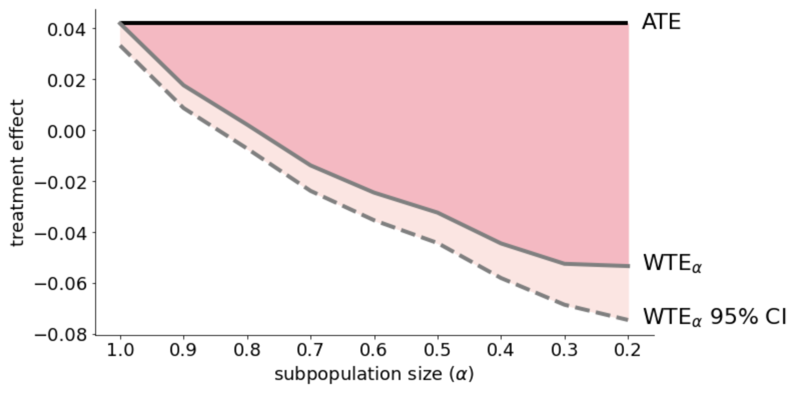
Figure 2: Effect of Medicaid enrollment on doctors visits in 2009

Using ten years of data (2009-18) from the National Health Interview Survey (NHIS), we focus on the binary outcome that indicates whether the individual made any visits to doctors in the two-weeks prior to the survey date [27, 55, 26, 48]. Although survey respondents have limited control on the outcome variable as the date of survey depends on the availability of field agents, Medicaid enrollments are nevertheless non-random. Those in poor health and higher intention of seeking treatment are more likely to enroll in Medicaid and thus more likely to visit the doctors, leading to an upward bias in confounded estimates. To address the potential bias, we control for a rich set of baseline covariates ($d=396$) including demographics, medical history, employment, earnings, health limitations, whether they require help with daily tasks, and enrollment status in insurance and government programs. We posit that there are no unobserved confounders (Assumption 1); as this is a strong assumption, we also study a randomized experiment in the following subsection. We restrict attention to the Census West region to ensure uniformity in the experiences of the control group across different states. Although Medicaid eligibility cannot be determined based on the NHIS survey data (number of family members is missing), we restrict attention to those with annual income $\leq$$65K so that respondents have a positive probability of eligibility.

The $\mbox{WTE}_{\alpha}$ (2) allows analyzing external validity over shifts in the study population. Using only data from 2009 ($n=82,993$ observations), in Figure 2 we plot the cross-fitted estimates of $\mbox{WTE}_{\alpha}$ across a range of subpopulation sizes $\alpha$. While the ATE is positive in 2009 (significant at 99%), observed effects fail to be significant even over subpopulations that comprise $\alpha=80\%$ of the study population. The WTE identifies subgroups disparately affected by the treatment and shows the average-case findings are invalidated under small changes to the study population. Our sensitivity framework thus brings into question whether the observed effects in 2009 can endure the test of time.

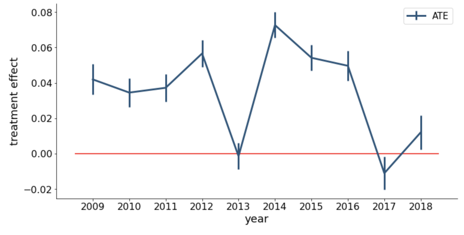
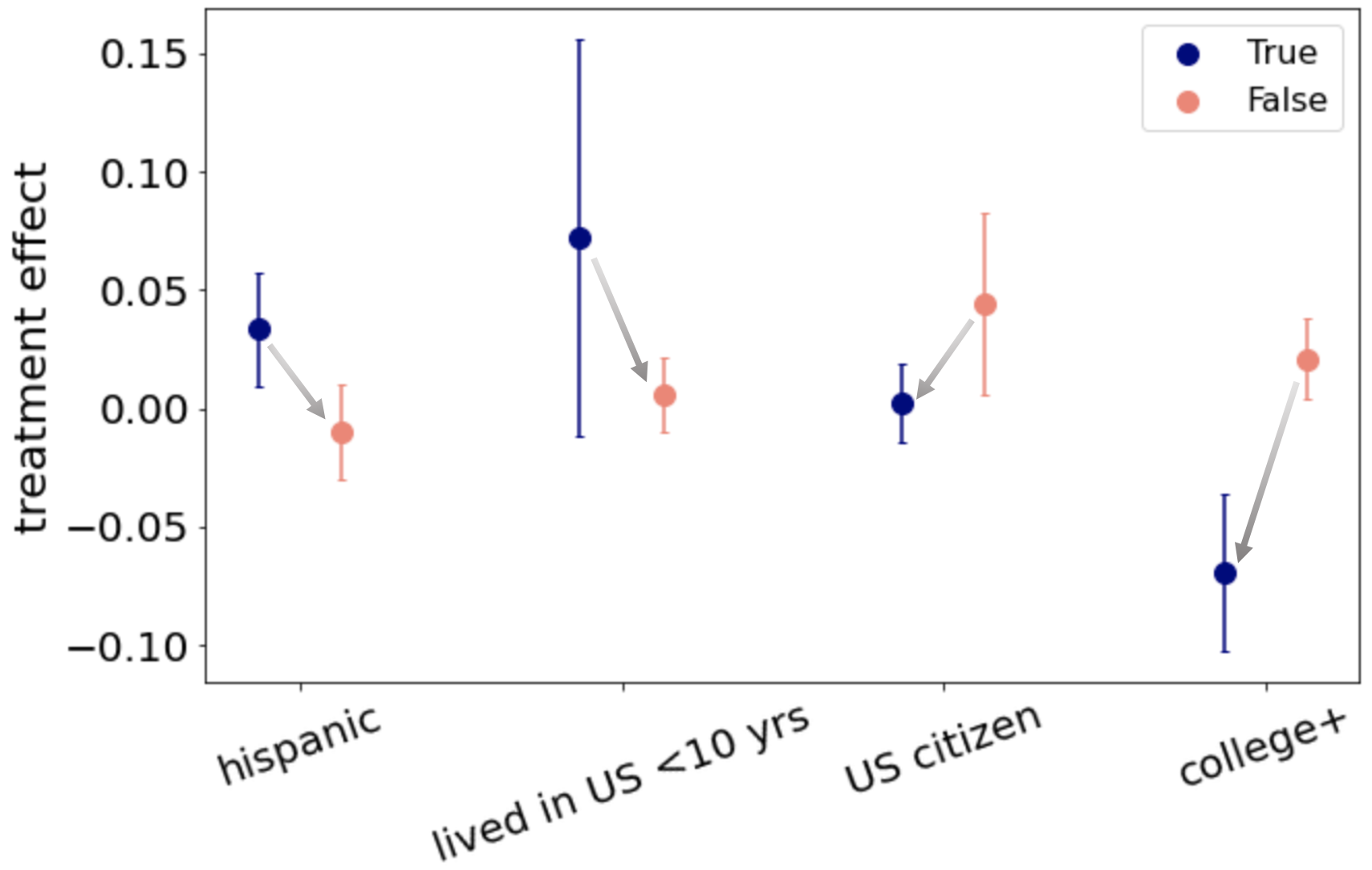
(a) ATE estimates in 2009-18 with 95% CIs	(b) CATE by covariates in 2009

Figure 3: Temporal changes in the ATE due to population shift

As predicted from 2009 data alone, treatment effects fail to be statistically significant over time (Figure 3a). To heuristically investigate the temporal population shift in the ATE, in Figure 1a we analyzed covariates with the largest mean difference between 2009 and 2018. The share of Hispanics and those who have been in the U.S. for less than 10 years decreased, but the share of U.S. citizens and those with high educational attainment increased. In Figure 3b, we observe that groups whose share decreased have higher treatment effects (and vice versa), contributing to the overall decrease in the treatment effect over time.

3.2 Welfare attitudes experiment

A large group of Americans harbors antipathy towards programs labeled “welfare,” a phenomenon that has generated much interest. We are interested in measuring how seemingly insubstantial wording changes in the description of social welfare programs affect public support. Disdain towards “welfare” has been associated with racist stereotypes towards welfare recipients [43, 36] and political ideology [51]. Previous works have observed substantial heterogeneity with respect to variables such as level of racism, education levels, and political leanings [47, 36, 40].

We study an experiment on welfare attitudes in the General Social Survey (GSS) from 1986 to 2010 [40]. We focus on the binary outcome indicating whether the respondents state too much is being spent on either “welfare” (treatment) or “assistance to the poor” (control). Both questions about public spending are identical except for the wording change. Covariates include attitude towards Blacks, political views, party identification, educational attainment, and age; there are $n=20,783$ data points, and $d=22$ covariates. To illustrate the flexibility of our estimation approach, we estimate the propensity score using a logistic regression with elastic net regularization as if it was unknown. (We observe similar results when we use the true propensity score $e^{\star}(X)\equiv\frac{1}{2}$.)

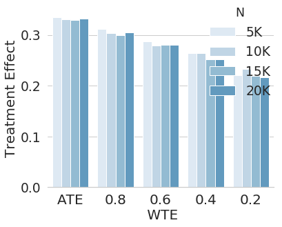
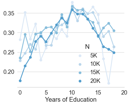
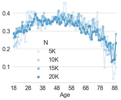
(a) ATE and WTEα	(b) CATE by years of education	(c) CATE by age

Figure 4: Treatment effects by number of observations.

By virtue of our semiparametric approach, we observe that even when CATE estimates vary significantly across sample size and outcome model classes, estimates of $\mbox{WTE}_{\alpha}$ align around a single value, a (empirical) stability property shared with estimators of ATE [18]. To illustrate the stability of WTE estimates, we plot them over different sample sizes (5-20K) and outcome model classes. Even at small sample sizes, wording changes in the survey have a resoundingly strong effect on attitude towards government welfare programs (Figure 4a). This observed effect is uniformly significant over subpopulations as small as 20% of the collected data. Such robust evidence instills confidence in the external validity of the finding across spatiotemporal changes in the demographic composition of respondents. While estimates of $\mbox{WTE}_{\alpha}$ and ATE remain relatively stable across different sample sizes, CATE estimates vary considerably over different sample sizes, a typical behavior for undersmoothed ML models (Figure 4b, c).

The stability of WTE estimates persists over different nuisance estimation approaches. Figure 5 explores several common model classes for the conditional outcome $\mathbb{E}[Y(z)\mid X]$: linear models with elastic net regularizers, random forests, and gradient boosted regression trees. All hyperparameters are chosen using 2-fold cross-validation as before. Figure 5a highlights the stability of WTE and ATE estimates along different models. In Figures 5b and c, we observe that CATE estimates vary up to 25 times, especially around the endpoint of bins, a common phenomenon often attributed to bias at the boundaries of the support of the feature space [83]. We anticipate that WTE estimators will similarly suffer instability issues when $\alpha$ is exceedingly small due to limited sample size.

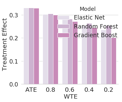
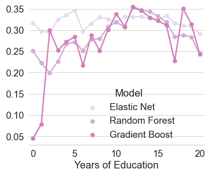
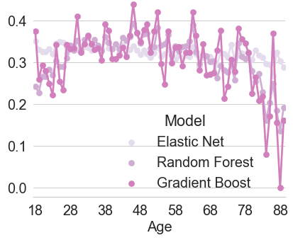
(a) ATE and WTEα	(b) CATE by years of education	(c) CATE by age

Figure 5: Treatment effects by model class.

4 Asymptotics

We now show that our cross-fitted augmented estimator (Algorithm 1) enjoys central limit behavior $\frac{\sqrt{n}}{\widehat{\sigma}_{\alpha}}(\widehat{\omega}_{\alpha}-\mbox{WTE}_{\alpha})\stackrel{{\scriptstyle d}}{{\rightsquigarrow}}N(0,1)$ even when we can only estimate the nuisance parameters (3) at slower-than-parametric rates. The Neyman orthogonality condition [60] serves a central role in our analysis.

Definition 1.

Let $Q\mapsto T(Q;\gamma)$ be a statistical functional with nuisance parameter $\gamma\in\Gamma$, where we take $\Gamma$ to be a subset of a normed vector space containing the true nuisance parameter $\gamma^{\star}$. The functional $T$ is Neyman orthogonal at $P$ if for all $\gamma\in\Gamma$, the derivative $\frac{d}{dr}\mathbb{E}_{P}[T(P;\gamma^{\star}+r(\gamma-\gamma^{\star}))]$ exists for $r\in[0,1)$, and is zero at $r=0$.

We use the augmented form (4) as our statistical functional $T(Q;\mu_{0},\mu_{1},e,h)$

$$T(Q;\mu_{0},\mu_{1},e,h):=\inf_{\eta}\left\{\frac{1}{\alpha}\mathbb{E}_{D\sim Q}\left({\mu(X)-\eta}\right)_{+}+\eta\right\}+\mathbb{E}_{D\sim Q}[\kappa(D;\mu_{0},\mu_{1},e,h)],$$ (7)

where we use $\mu(x):=\mu_{1}(x)-\mu_{0}(x)$ as usual. The first term is the dual form of $\mbox{WTE}_{\alpha}$ (Lemma 1), and the second term is the augmentation term defined in Eq. (4). Since $\mathbb{E}_{D\sim P}[\kappa(D;\mu_{0}^{\star},\mu_{1}^{\star},e^{\star},h^{\star})]=0$ under ignorability (Assumption 1), we have $T(P;\mu_{0}^{\star},\mu_{1}^{\star},e^{\star},h^{\star})=\mbox{WTE}_{\alpha}$.

To build intuition, we first informally argue that this augmented functional satisfies Neyman orthogonality. We first compute the (Gateaux) derivative of the first dual infimization term in the functional (7). From Danskin’s theorem [16, Theorem 4.13], the derivative of the dual formulation is the derivative of the objective at the unique optimal solution. Under sufficient regularity conditions, the unique solution to the dual is given by the quantile $P_{1-\alpha}^{-1}(\mu^{\star})$, and the derivative at $r=0$ is

$$\frac{d}{dr}\inf_{\eta}\left\{\frac{1}{\alpha}\mathbb{E}\left({(\mu^{\star}+r(\mu-\mu^{\star}))(X)-\eta}\right)_{+}+\eta\right\}\Bigg{|}_{r=0}=\mathbb{E}[h^{\star}(X)(\mu-\mu^{\star})(X)].$$

To compute the derivative of the second term, let $\gamma=(\mu_{0},\mu_{1},e,h)$ to ease notation. So long as we can interchange derivatives and expectations, it is straightforward to calculate

$$\frac{d}{dr}\mathbb{E}\left[\kappa\left(D;\gamma^{\star}+r(\widehat{\gamma}_{k}-\gamma)^{\star}\right)\right]|_{r=0}=-\mathbb{E}[h^{\star}(X)(\mu-\mu^{\star})(X)]$$

from ignorability (Assumption 1). This verifies Neyman orthogonality of the functional (7).

Orthogonality allows us to show a central limit theorem for our augmented cross-fitting estimator $\widehat{\omega}_{\alpha}$ under the following weak rate requirements for the nuisance parameters. Recall the bound $c>0$ on the propensity score given in Assumption 2.

Assumption 4.

Let $\left\|{\widehat{\mu}_{k}-\mu^{\star}}\right\|_{L^{1}(\mathcal{X})}\stackrel{{\scriptstyle a.s.}}{{\rightarrow}}0$, and let there exist an envelope function $\bar{\mu}:\mathcal{X}\to\mathbb{R}$ satisfying $\mathbb{E}[\bar{\mu}(X)^{2}]<\infty$ and $\max(|\widehat{\mu}_{0,k}|,|\widehat{\mu}_{1,k}|)\leq\bar{\mu}$. There exists $\delta_{n},\Delta_{n}\downarrow 0$, and $M_{h}>0$ such that with probability at least $1-\Delta_{n}$, for all $k\in[K]$

1. $\left\|{\widehat{e}_{k}-e^{\star}}\right\|_{L^{2}(\mathcal{X})}+\left\|{\widehat{\mu}_{0,k}-\mu_{0}^{\star}}\right\|_{L^{2}(\mathcal{X})}+\left\|{\widehat{\mu}_{1,k}-\mu_{1}^{\star}}\right\|_{L^{2}(\mathcal{X})}\leq\delta_{n}$, $\widehat{e}_{k}\in[c,1-c]$, and $|\widehat{h}_{k}|\leq M_{h}$

2. $\left\|{\widehat{e}_{k}-e^{\star}}\right\|_{L^{2}(\mathcal{X})}\left(\left\|{\widehat{\mu}_{0,k}-\mu_{0}^{\star}}\right\|_{L^{2}(\mathcal{X})}+\left\|{\widehat{\mu}_{1,k}-\mu_{1}^{\star}}\right\|_{L^{2}(\mathcal{X})}\right)\leq\delta_{n}n^{-1/2}$

3. $\left\|{\widehat{\mu}_{k}-\mu^{\star}}\right\|_{L^{\infty}(\mathcal{X})}\leq\delta_{n}n^{-1/3}$, and $|\widehat{q}_{k}-P_{1-\alpha}^{-1}(\widehat{\mu}_{k})|\leq\delta_{n}n^{-1/3}$

In particular, Assumption 4 does not require a $\sqrt{n}$-convergence rate (Donsker condition) on the estimators of nuisance parameters. The first two conditions are standard convergence rates [22], also required for proving a central limit result for the ATE. They hold, in particular, when $\left\|{\widehat{e}-e^{\star}}\right\|_{L^{2}(\mathcal{X})}=o_{p}(n^{-1/4})$ and $\left\|{\widehat{\mu}_{z}-\mu^{\star}_{z}}\right\|_{L^{2}(\mathcal{X})}=o_{p}(n^{-1/4})$ for $z\in\{0,1\}$. The third condition guarantees approximation of the threshold function $h^{\star}(x)=\alpha^{-1}\mathbf{1}\left\{\mu^{\star}(x)\geq P_{1-\alpha}^{-1}(\mu^{\star})\right\}$ at suitably fast rates. The requirement $\left\|{\widehat{\mu}_{k}-\mu^{\star}}\right\|_{L^{\infty}(\mathcal{X})}\leq\delta_{n}n^{-1/3}$ states that the CATE be estimated at a somewhat faster rate compared to the case for estimating the ATE. In Appendix A, we provide detailed examples of model classes and learning methods where these convergence rates hold. As noted in Section 2, when unlabeled covariates (those without corresponding outcomes nor treatments) are cheaply available, the second part of $(c)$ can be easily achieved.

As the WTE is a tail-average of the CATE above the quantile $P_{1-\alpha}^{-1}(\mu^{\star})$ (recall Lemma 1), to estimate $\mbox{WTE}_{\alpha}$ we need to estimate the quantile $P_{1-\alpha}^{-1}(\mu^{\star})$. Towards this goal, we require that a positive density exists at its $(1-\alpha)$-quantile, a standard condition required for quantile estimation [82, Chapter 3.7]. Let $\mathcal{U}$ be a subset of measurable functions $\mu:\mathcal{X}\to\mathbb{R}$ such that the following holds:

$F_{r,\mu}$, the cumulative distribution of $(\mu^{\star}+r(\mu-\mu^{\star}))(X)$, is uniformly differentiable in $r\in[0,1]$ at $P_{1-\alpha}^{-1}(\mu^{\star}+r(\mu-\mu^{\star}))$, with a positive density. Formally, if we let $q_{r,\mu}:=P_{1-\alpha}^{-1}(\mu^{\star}+r(\mu-\mu^{\star}))$, then for each $r\in[0,1]$, there is a positive density $f_{r,\mu}(q_{r,\mu})>0$ such that

$$\lim_{t\to 0}\sup_{r\in[0,1]}\left|\frac{1}{t}\left(F_{r,\mu}(q_{r,\mu}+t)-F_{r,\mu}(q_{r,\mu})\right)-f_{r,\mu}(q_{r,\mu})\right|=0.$$ (8)

We require this holds for our estimators $\mu=\widehat{\mu}_{k}$ with high probability.

Assumption 5.

$\exists\Delta_{n}^{\prime}\downarrow 0$ s.t. with probability at least $1-\Delta_{n}^{\prime}$, $\widehat{\mu}_{k}\in\mathcal{U}$ for all $k\in[K]$.

In particular, Assumption 5 requires $\mu^{\star}(X)$ to have a positive density at $P_{1-\alpha}^{-1}(\mu^{\star})$.

We are now ready to give our main technical result which shows that the augmented cross-fitting estimator $\widehat{\omega}_{\alpha}$ enjoys central limit rates with the influence function

$$\psi(D):=\frac{1}{\alpha}\left({\mu^{\star}(X)-P_{1-\alpha}^{-1}(\mu^{\star})}\right)_{+}+P_{1-\alpha}^{-1}(\mu^{\star})-\mbox{WTE}_{\alpha}+\kappa\left(D;\mu_{0}^{\star},\mu_{1}^{\star},e^{\star},h^{\star}\right).$$ (9)

Indeed, $\psi(D)$ is a valid influence function under Assumption 1: we have $\mathbb{E}[\psi(D)]=0$, and ${\rm Var}(\psi(D))=\sigma^{2}_{\alpha}$ where $\sigma_{\alpha}^{2}$ is the asymptotic variance defined in expression (5).

Theorem 1.

Under Assumptions 1-5, $\sqrt{n}(\widehat{\omega}_{\alpha}-\mbox{WTE}_{\alpha})=\frac{1}{\sqrt{n}}\sum_{i=1}^{n}\psi(D_{i})+o_{p}(1)$. Further, we have $\widehat{\sigma}^{2}_{\alpha}\stackrel{{\scriptstyle p}}{{\rightarrow}}\sigma^{2}_{\alpha}$ and $\frac{\sqrt{n}}{\widehat{\sigma}_{\alpha}}(\widehat{\omega}_{\alpha}-\mbox{WTE}_{\alpha})\stackrel{{\scriptstyle d}}{{\rightsquigarrow}}N(0,1)$.

Since the proof of Theorem 1 is involved, we give its sketch below, emphasizing how we leverage Neyman orthogonality of the augmented functional (7) to obtain our result. We provide rigorous details of the proof in Appendices B, C, D. Chernozhukov et al. [22] showed that the solution of a Neyman orthogonal estimating equation could be estimated at the usual central limit rate, even when nuisance parameters converge at slower rates. Their results do not apply to the $\mbox{WTE}_{\alpha}$ as it is a nonlinear statistical functional of the underlying probability measure $P$. To account for such nonlinearity, our theoretical analysis considerably extends existing results. Using tools from empirical process theory [82], our main result shows that for uniformly Hadamard differentiable functionals, orthogonality still allows insensitivity to estimation error in nuisance parameters. Even when $\alpha=100\%$ so that $\mbox{WTE}_{1}=\mbox{ATE}$ and our estimator reduces to the cross-fitted AIPW for the ATE, our argument provides a different proof to that given by Chernozhukov et al. [22].

Sketch of proof for Theorem 1

Our proof proceeds in three parts. Recalling $\widehat{P}_{k}$, the empirical distribution on the $k$-th fold, our cross-fitted estimator can be written succinctly as $\frac{1}{K}\sum_{k=1}^{K}T(\widehat{P}_{k};\widehat{\mu}_{0,k},\widehat{\mu}_{1,k},\widehat{e}_{k},\widehat{h}_{k})$. We emphasize (empirical) expectations over $Q$ in the definition (7) are taken only over $D$, and not over the randomness in $(\widehat{\mu}_{0,k},\widehat{\mu}_{1,k},\widehat{e}_{k},\widehat{h}_{k})$.

The first two parts show that for each fold $k\in[K]$,

$$\sqrt{|I_{k}|}\left(T\left(\widehat{P}_{k};\widehat{\mu}_{0,k},\widehat{\mu}_{1,k},\widehat{e}_{k},\widehat{h}_{k}\right)-T(P;\mu_{0}^{\star},\mu_{1}^{\star},e^{\star},h^{\star})\right)=\frac{1}{\sqrt{|I_{k}|}}\sum_{i\in I_{k}}\psi(D_{i})+o_{p}(1).$$ (10)

Since $T(P;\mu_{0}^{\star},\mu_{1}^{\star},e^{\star},h^{\star})=\mbox{WTE}_{\alpha}$ by ignorability (Assumption 1), this gives our first result. Towards this goal, decompose the left hand side of the equality (10) into

$$\sqrt{|I_{k}|}\left(T\left(\widehat{P}_{k};\widehat{\mu}_{0,k},\widehat{\mu}_{1,k},\widehat{e}_{k},\widehat{h}_{k}\right)-T\left(P;\widehat{\mu}_{0,k},\widehat{\mu}_{1,k},\widehat{e}_{k},\widehat{h}_{k}\right)\right)$$ (11a)

$$+\sqrt{|I_{k}|}\left(T\left(P;\widehat{\mu}_{0,k},\widehat{\mu}_{1,k},\widehat{e}_{k},\widehat{h}_{k}\right)-T(P;\mu_{0}^{\star},\mu_{1}^{\star},e^{\star},h^{\star})\right).$$ (11b)

In Part I of the proof (Appendix B), we prove that the first term (11a) is asymptotically equal to $\frac{1}{\sqrt{|I_{k}|}}\sum_{i\in I_{k}}\psi(D_{i})$. Leveraging tools from empirical process theory [82], we first show that the functional $Q\mapsto T(Q;\widehat{\mu}_{0,k},\widehat{\mu}_{1,k},\widehat{e}_{k},\widehat{h}_{k})$ satisfies a uniform variant of Hadamard differentiability so that the functional delta method applies. A careful application of a uniform version of the Lindeberg-Feller central limit theorem over functions gives the desired conclusion.

In Part II (Appendix C), we use Neyman orthogonality of our augmented estimator to show that the second term (11b) vanishes asymptotically. Define $\mathfrak{R}_{k}:[0,1]\to\mathbb{R}$

$$\mathfrak{R}_{k}(r):=T\left(P;(1-r)(\mu_{0}^{\star},\mu_{1}^{\star},e^{\star},h^{\star})+r(\widehat{\mu}_{0,k},\widehat{\mu}_{1,k},\widehat{e}_{k},\widehat{h}_{k})\right)-T(P;\mu_{0}^{\star},\mu_{1}^{\star},e^{\star},h^{\star}),$$ (12)

so that $\mathfrak{R}_{k}(0)=0$, and $\mathfrak{R}_{k}(1)$ is equal to the second term (11b). $\mathfrak{R}_{k}(r)$ is continuously differentiable under suitable conditions and mean value theorem gives

$$\mathfrak{R}_{k}(1)=\mathfrak{R}_{k}(0)+\mathfrak{R}_{k}^{\prime}(r)\cdot(1-0)=\mathfrak{R}_{k}^{\prime}(r)$$

for some $r\in[0,1]$. From Neyman orthogonality, we have $\mathfrak{R}_{k}^{\prime}(0)=0$. Building on this, we show that all values of $\mathfrak{R}_{k}^{\prime}(r)$ are sufficiently small: under postulated convergence rates for the nuisance parameters in Assumption 4, $\sup_{r\in[0,1]}|\mathfrak{R}_{k}^{\prime}(r)|=o_{p}(n^{-1/2})$.

In Part III (Appendix D), we show consistency of our variance estimator: $\widehat{\sigma}^{2}_{\alpha}\stackrel{{\scriptstyle p}}{{\rightarrow}}\sigma^{2}_{\alpha}$. Combining this with the central limit result (10), Slutsky’s lemma gives our second result. $\diamond$

5 Semiparametric efficiency bound

We now establish a semiparametric efficiency bound, showing that all (regular) estimators of $\mbox{WTE}_{\alpha}$ necessarily have asymptotic variance larger than $\sigma_{\alpha}^{2}$, both when the true propensity score $e^{\star}(\cdot)$ is known and unknown. In particular, this implies that our augmented estimator $\widehat{\omega}_{\alpha}$ achieves the optimal asymptotic variance and that its influence function (9) is the efficient influence function for estimating $\mbox{WTE}_{\alpha}$. Our efficiency bound i) informs the design of experiments by providing the minimum number of study participants required to reach a conclusion that is valid across subpopulations no smaller than $\alpha$ and ii) quantifies how the required sample size grows with the level of desired external validity $\alpha$.

For parametric problems, Hajek-Le Cam theorems [81, Chapter 8] give a lower bound on the asymptotic variance of regular estimators, more generally, a lower bound on the mean squared error for any estimator. Since these bounds coincide with the Cramer-Rao bound for unbiased estimators, they can be considered as an asymptotic Cramer-Rao bound. We consider parametric submodels of our semiparametric problem, i.e., finite-dimensional parameterizations that contain the truth. Since the asymptotic variance of any (smooth enough) semiparametric estimator is worse than the Hajek-Le Cam bound—equivalently, the Cramer-Rao bound—of any parametric submodel, the semiparametric efficiency bound is defined as the supremum of the Hajek-Le Cam bound over all parametric submodels. As these definitions are standard yet tedious [59, 14], we defer a formal treatment to Appendix E.

We now characterize the semiparametric efficiency bound for estimating $\mbox{WTE}_{\alpha}$.

Assumption 6.

$\mu^{\star}(X)$ has a positive density, and $\left\|{\mathbb{E}[|Y(z)|\mid X]}\right\|_{L^{\infty}(\mathcal{X})}<\infty$, $z\in\{0,1\}$.

Theorem 2.

Let Assumptions 1, 2, 3, 6 hold, and $\sigma^{2}_{\alpha}=\mathbb{E}[\psi(D)^{2}]>0$, where $\psi$ was defined in Eq. (9). Then, $\mbox{WTE}_{\alpha}$ is a differentiable parameter in the sense of Definition 5, and its semiparametric efficiency bound is given by $\mathbb{E}[\psi(D)^{2}]$. The efficiency bound is identical if the true propensity score is known.

See Appendix E for the proof. Theorem 1 and 2 show that our cross-fitted augmented estimator $\widehat{\omega}_{\alpha}$ achieves the semiparametric efficiency bound $\mathbb{V}(\mbox{WTE}_{\alpha};P)$. Similar to the efficiency bound for the ATE [41], the knowledge of $e^{\star}(\cdot)$ does not affect the efficiency bound $\mathbb{V}(\mbox{WTE}_{\alpha};P)$. We conclude that our estimator is semiparametrically efficient for both observational studies and randomized control trials.

Our semiparametric efficiency bound allows calculating the minimum required sample size for finding conclusions that are robust against all subpopulations of size at least $\alpha$. Consider the hypothesis test $H_{0}:\mbox{WTE}_{\alpha}\geq 0~{}\mbox{v.}~{}H_{\rm A}:\mbox{WTE}_{\alpha}<-\epsilon$, where $\epsilon>0$ is the specified minimum detectable effect size (recall that the desired sign of the treatment effect is negative). As an illustration, consider a test with size ($\mathbb{P}(\mbox{Type I error})$) at most $5\%$ and power ($1-\mathbb{P}(\mbox{Type II error})$) at least $80\%$. A standard power calculation shows $n\geq 6.2\frac{\sigma_{\alpha}^{2}}{\epsilon^{2}}$ samples are needed to detect a worst-case subpopulation treatment effect of size $-\epsilon$. In particular, this number grows as we require a stronger level of external validity, or equivalently as the worst-case subpopulation size $\alpha$ becomes small.

6 Discussion

Motivated by challenges in evaluating treatments under unanticipated population shifts, we proposed a sensitivity analysis framework based on the worst-case subpopulation treatment effect. We advocate for such conservatism in important policy decisions that need to benefit all subpopulations uniformly. While the WTE (2) provides a strong notion of robustness, it may be overly conservative in scenarios where one is concerned with more structured covariate shifts. When covariate shift on only a small subset of $X$ is of interest, the definition (2) can be modified over this subset. More broadly, studying structured shifts in the covariate distribution $P_{X}$ is an exciting direction of future work.

Our theoretical developments show that our cross-fitted augmented estimator inherits two advantageous inferential properties of the AIPW estimator for the ATE: orthogonality and efficiency. Elementary derivations show, however, that our estimator does not satisfy the doubly robust property due to the additional nuisance parameter $h^{\star}(x)=\alpha^{-1}\mathbf{1}\left\{\mu^{\star}(x)\geq P_{1-\alpha}^{-1}(\mu^{\star})\right\}$. Another limitation of our augmented estimator is that it is not necessarily increasing in $\alpha$. Though the extension of the direct method and the inverse probability weighted estimator are increasing in $\alpha$, it is unclear whether an orthogonal, efficient, and monotone estimator of the WTE exists. Finally, estimators of tail-averages often suffer higher variance and may be more sensitive to lack of overlap and unobserved confounding. Further investigation of these issues is a topic for future research.

Sometimes it is of interest to estimate the average treatment effect on the treated $\mathbb{E}[Y(1)-Y(0)\mid Z=1]$. There are two natural ways to extend the worst-case definition (2) to measure the effect on the treated, depending on whether the worst-case is still taken over $Q_{X}$, or over the conditional distribution $Q_{X\mid Z=1}$. We leave a systematic study of the two definitions and corresponding inferential frameworks to future work.

Acknowledgments

We thank Steve Yadlowsky for helpful comments.

Notation

Throughout, we let $F_{\mu}$ denote the cumulative distribution of $\mu(X)$, and let $P_{1-\alpha}^{-1}(\mu):=\inf\{t:F_{\mu}(t)\geq 1-\alpha\}$ be the $(1-\alpha)$-quantile of $\mu(X)$; when $\mu(\cdot)$ is random (e.g. estimated from data), the probabilities are taken only over $X\sim P$. $L^{q}(\mathcal{X})$ is the $L^{q}$ norm w.r.t. $X\sim P$. For $a_{n}\in\mathbb{R}$, we write $X_{n}=O_{P}(a_{n})$ if $\lim_{b\to\infty}\limsup_{n}P(|X_{n}|\geq b\cdot a_{n})=0$, and $X_{n}=o_{P}(a_{n})$ if $\limsup P(|X_{n}|\geq b\cdot a_{n})=0$ $\forall b>0$.

Appendix A Review of nuisance estimation approaches

In this section, we review standard loss minimization approaches to estimating the nuisance parameters $\mu_{1}^{\star},\mu_{0}^{\star},e^{\star}$. For ease of exposition, we focus on estimation of $\mu_{1}^{\star}=\mathbb{E}[Y(1)|X=x]$; directly analogous results are available for $\mu_{0}^{\star}$ and $e^{\star}$. Our starting point is the fact that $\mu_{1}^{\star}$ is the solution to the loss minimization problem

$$\mathop{\rm minimize}_{\mu_{1}(\cdot):~{}\mbox{\scriptsize measurable}}\mathbb{E}[(Y-\mu_{1}(X))^{2}\mid Z=1].$$ (13)

We consider empirical plug-in estimators $\widehat{\mu}_{1,k}$ on the auxiliary sample $I_{k}^{c}$, given by the (approximate) solution to the following optimization problem

$$\mathop{\rm minimize}_{\mu_{1}}\sum_{i\in I_{k}^{c}}Z_{i}(Y_{i}-\mu_{1}(X_{i}))^{2},$$ (14)

where the minimization problem is taken over a suitably chosen (possibly regularized) model class.

The guarantees we focus on below scale separately in the complexity of model classes for $\widehat{\mu}_{1,k}$ and $\widehat{\mu}_{0,k}$. On the other hand, our most stringent rate requirement $\left\|{\widehat{\mu}_{k}-\mu^{\star}}\right\|_{L^{\infty}(\mathcal{X})}=o_{p}(n^{-1/3})$ only requires convergence of $\widehat{\mu}_{k}=\widehat{\mu}_{1,k}-\widehat{\mu}_{0,k}$; see Künzel et al. [53] for procedures that scale with the complexity of $\widehat{\mu}_{k}$, which are advantageous when $\mu^{\star}$ has significantly lower complexity than $\mu_{1}^{\star}$ and $\mu_{0}^{\star}$.

A.1 High-dimensional estimation

We consider two typical estimation scenarios involving high dimensional covariates $X$. Our guarantees in this subsection require that the model class $\mathcal{M}$ we optimize over in the empirical problem (14) be well-specified (i.e., $\mu_{1}^{\star}\in\mathcal{M}$). We relax this condition in Section A.2, where we consider nonparameteric estimators.

Example 1 (Sparse linear regresion):  Consider the sparse linear regression problem

$$Y(1)=\theta^{\star\top}X+\varepsilon,$$

where $\varepsilon\rotatebox[origin={c}]{90.0}{$\models$}X$, $\mathbb{E}[\epsilon]=0$, and $\left\|{\varepsilon}\right\|_{\infty}\leq 1$ (so that $\mu_{1}^{\star}(X)=\theta^{\star\top}X$). We consider the scenario where $\theta^{\star}$ is $s$-sparse, $\left\|{\theta^{\star}}\right\|_{0}\leq s$, and satisfies $\left\|{\theta^{\star}}\right\|_{1}\leq 1$. We assume $\left\|{X}\right\|_{\infty}\leq 1$ a.s. for simplicity.

Let $\widehat{\mu}_{1,k}$ be the solution to the empirical optimization problem (14) over the model class

$$\mathcal{M}=\left\{x\mapsto\theta^{\top}x:\left\|{\theta}\right\|_{0}\leq s,\left\|{\theta}\right\|_{1}\leq 1\right\}.$$

A standard localized Rademacher complexity argument [10, 84] and another standard covering bound over a class of linear functions [85, 82] show that with probability at least $1-\Delta$,

$$\left\|{\widehat{\mu}_{1,k}-\mu_{1}^{\star}}\right\|_{L^{2}(\mathcal{X})}=O\left(\sqrt{\frac{s\log(d/s)}{n}}+\sqrt{\frac{\log(1/\Delta)}{n}}\right).$$

We conclude that the rate requirements for $\widehat{\mu}_{1,k}$ given in Assumption 4 hold whenever $s\log d\ll n^{1/3}$.

Similar rates can be shown for the (convex) Lasso-regularized model class $\{x\mapsto\theta^{\top}x:\left\|{\theta}\right\|_{1}\leq\left\|{\theta^{\star}}\right\|_{1}\}$ under the standard restricted eigenvalue conditions on $\{X_{i}\}_{i\in I_{k}^{c}}$. Variants of these results can also be shown when these norm constraints appear as regularizers in the objective. We refer the reader to Wainwright [84] and Hastie et al. [42, Chapter 11] for a detailed overview of related results. $\diamond$

Example 2 (Neural networks):  Consider neural networks with ReLU activations $v(a)=\max(a,0)$

$$\mathcal{M}=\left\{\mu_{1}(x)=A_{L}v\left(A_{L-1}v\left(\cdots v\left(A_{1}x\right)\cdots\right)\right):A_{l}\in\mathbb{R}^{d_{l}\times d_{l-1}},\left\|{\mu_{1}}\right\|_{L^{\infty}(\mathcal{X})}\leq C\right\},$$

where $d_{0}=d$ and $d_{L}=1$. We assume that the depth of the network, $L$, is deep enough to represent the true parameter $\mu_{1}^{\star}$ so that $\mu_{1}^{\star}\in\mathcal{M}$ and $Y(1)=\mu_{1}^{\star}(X)+\varepsilon$, where $\varepsilon\rotatebox[origin={c}]{90.0}{$\models$}X$, $\mathbb{E}[\epsilon]=0$, and $\left\|{\varepsilon}\right\|_{\infty}\leq 1$.

Let $d_{\mathcal{M}}=\prod_{l=1}^{L}d_{l}d_{l-1}$ be the number of parameters in the neural network. Again, standard a localized Rademacher complexity argument [10, 84] and bounds on the VC dimension for neural networks [11, Theorem 6] yields

$$\left\|{\widehat{\mu}_{1,k}-\mu_{1}^{\star}}\right\|_{L^{2}(\mathcal{X})}=O\left(\sqrt{\frac{d_{\mathcal{M}}L\log d_{\mathcal{M}}\log C}{n}}+\sqrt{\frac{\log(1/\Delta)}{n}}\right)$$

with probability at least $1-\Delta$. Rate requirements for $\widehat{\mu}_{1,k}$ given in Assumption 4 hold whenever $d_{\mathcal{M}}L\log d_{\mathcal{M}}\log C\ll n^{1/3}$. $\diamond$

A.2 Sieve estimation

We now move away from well-specified parametric approaches, and consider nonparametric sieve estimators that take an increasing sequence $\mathcal{M}_{n}\subset\mathcal{M}_{n+1}\subset\cdots\subset\mathcal{M}^{\star}$ of spaces of functions as the model class in the empirical optimization problem (14) [38]. We let $\mathcal{M}^{\star}$ be the (nonparametric) set of suitably smooth functions, and only require that $\mu_{1}^{\star}\in\mathcal{M}^{\star}$, allowing very general class of functions and misspecified model classes $\mathcal{M}_{n}$. By appropriately choosing the approximation space $\mathcal{M}_{n}$, which we call sieves, we can provide estimation guarantees required in Assumption 4 whenever $\mu_{1}^{\star}$ is smooth enough. We refer the reader to Chen [20] for a detailed overview of sieve estimators.

For concreteness, we consider the following sieve spaces.
Example 3 (Polynomials):  Let $\mbox{Pol}\left(J\right)$ be the space of $J$-th order polynomials on $[0,1]$

$$\mbox{Pol}\left(J\right):=\left\{[0,1]\ni x\mapsto\sum_{k=0}^{J}a_{k}x^{k}:a_{k}\in\mathbb{R}\right\},$$

and let the sieve be $\mathcal{M}_{n}:=\left\{x\mapsto\Pi_{k=1}^{d}f_{k}(x_{k})\mid f_{k}\in\mbox{Pol}\left(J_{n}\right),k=1,\dots,d\right\},$ for $J_{n}\to\infty$. $\diamond$

Example 4 (Splines):  Consider knots $0=t_{0}<\ldots<t_{J+1}=1$ such that

$$\frac{\max_{0\leq j\leq J}(t_{j+1}-t_{j})}{\min_{0\leq j\leq J}(t_{j+1}-t_{j})}\leq c$$

for some $c>0$. Let space of $r$-th order splines with $J$ knots be

$$\mbox{Spl}\left(r,J\right):=\left\{x\mapsto\sum_{k=0}^{r-1}a_{k}x^{k}+\sum_{j=1}^{J}b_{j}\left({x-t_{j}}\right)_{+}^{r-1},x\in[0,1]:a_{k},b_{k}\in\mathbb{R}\right\},$$

and the corresponding sieve $\mathcal{M}_{n}:=\left\{x\mapsto f_{1}(x_{1})f_{2}(x_{2})\dots f_{d}(x)\mid f_{k}\in\mbox{Spl}\left(r,J_{n}\right),k=1,\dots,d\right\}$ for some integer $r\geq\left\lfloor{p}\right\rfloor+1$ and $J_{n}\to\infty.$ $\diamond$

The empirical approximation (14) over $\mu_{1}\in\mathcal{M}_{n}$ is a convex optimization problem when $\mathcal{M}_{n}$ is a finite dimensional linear space, as in Examples A.2 or A.2.

We also consider neural networks with one hidden layer, without requiring that the model class is well-specified as in Section A.1.
Example 5 (Neural network with one hidden layer):  Consider neural networks with one hidden layer, with the sigmoid activation function $v(a)=(1+\exp^{-a})^{-1}$

$$\mathcal{M}_{n}:=\left\{x\mapsto a_{0}+\sum_{j=1}^{J_{n}}a_{j}v(b_{j}^{\top}x+b_{0,j}):a_{j},b_{0,j}\in\mathbb{R},b_{j}\in\mathbb{R}^{d},\max\left(\sum_{j=0}^{J_{n}}|a_{j}|,\max_{1\leq j\leq J_{n}}\sum_{i=0}^{d}|b_{ij}|\right)\leq C\right\},$$

for some $C>0$ and $J_{n}\to\infty$. $\diamond$

To establish asymptotic convergence of $\widehat{\mu}_{1,k}$, we need some regularity conditions. First, we assume a condition that allows control of supremum norm errors using the $L^{2}(P)$-norm. This is an important requirement used to show convergence [20] of sieve estimators.

Assumption 7.

Let $P_{X|Z=1}$ have density $p_{1}(x)$ with respect to the Lebesgue measure, such that $0<\inf_{x\in\mathcal{X}}p_{1}(x)\leq\sup_{x\in\mathcal{X}}p_{1}(x)<\infty$.

For the first two examples, we will assume that $\mu_{1}^{\star}$ belong in a Hölder class. Recall that the Hölder class $\Lambda^{p}_{R}(\mathcal{X})$ of $p$-smooth functions for $p_{1}=\left\lceil{p}\right\rceil-1$ and $p_{2}=p-p_{1}$ is given by

$$\Lambda^{p}_{R}(\mathcal{X}):=\left\{h\in C^{p_{1}}(\mathcal{X}):\sup_{\tiny\begin{array}[]{c}x\in\mathcal{X}\\ \sum_{l=1}^{d}\alpha_{l}<p_{1}\end{array}}|D^{\alpha}h(x)|+\sup_{\tiny\begin{array}[]{c}x\neq x^{\prime}\in\mathcal{X}\\ \sum_{l=1}^{d}\beta_{l}=p_{1}\end{array}}\frac{|D^{\beta}h(x)-D^{\beta}h(x^{\prime})|}{\left\|{x-x^{\prime}}\right\|^{p_{2}}}\leq R.\right\},$$

where $C^{p_{1}}(\mathcal{X})$ denotes the space of $p_{1}$-times continuously differentiable functions on $\mathcal{X},$ and $D^{\alpha}=\frac{\partial^{\alpha}}{\partial^{\alpha_{1}}\ldots\partial^{\alpha_{d}}}$, for any $d$-tuple of nonnegative integers $\alpha=(\alpha_{1},\ldots,\alpha_{d})$.

Assumption 8.

Let $\mathcal{X}=\mathcal{X}_{1}\times\cdots\times\mathcal{X}_{d}$ be the Cartesian product of compact intervals $\mathcal{X}_{1},\ldots,\mathcal{X}_{d}$, and assume $\mu_{1}^{\star}\in\Lambda^{p}_{R}(\mathcal{X})=:\mathcal{M}^{\star}$ for some $R>0$.

The assumption $\mu_{1}^{\star}\in\Lambda^{p}_{R}(\mathcal{X})$ allows general functions $\mu_{1}^{\star}$ while ensuring it is well-approximated by finite dimensional linear sieves. In particular, sieve spaces in Examples A.2 and A.2 achieve approximation error $\inf_{\mu_{1}\in\mathcal{M}_{n}}\left\|{\mu_{1}-\mu_{1}}\right\|_{\infty}=O(J_{n}^{-p})$ (see, e.g., [75, Sec. 5.3.1] or [71, Thm. 12.8]). Similar guarantees also hold for wavelet bases (as well as others) [29, 20], though we omit it for brevity.

By choosing $J_{n}$ to optimally trade off statistical estimation error and approximation error, we can achieve optimal nonparametric convergence rates. The following theorem is a straightforward consequence of Chen and Shen [21].

Lemma 2 (Chen and Shen [21]).

For $\mathcal{X}=[0,1]^{d}$, consider $\mathcal{M}_{n}$ in Example A.2 or A.2 with $J_{n}\asymp n^{\frac{1}{2p+d}}$. Let Assumptions 3, 8, 7 hold, and let $\widehat{\mu}_{1,k}$ be a $O_{p}\left(\left(\frac{\log n}{n}\right)^{\frac{2p}{2p+d}}\right)$-approximate optimizer of the empirical problem (14). Then, we have $\|{\widehat{\mu}_{1}-\mu_{1}}\|_{2,P}=O_{p}\left(\left(\frac{\log n}{n}\right)^{\frac{p}{2p+d}}\right)$.

The above result states that when $p>d$, that is when $\mu_{1}^{\star}$ is sufficiently smooth relative to the dimension, relevant requirements in Assumption 4 are satisfied.

For neural networks with one hidden layer, we have the following result which builds out of universal approximation guarantees shown by Barron [9] and Makovoz [56].

Lemma 3 (Chen and Shen [21]).

Let Assumptions 3, 7 hold, and let $\mu_{1}^{\star}$ be given by $\mu_{1}^{\star}(x)=\int\exp(ia^{\top}x)d\nu(a)$ for some complex valued measure $\nu$ on $\mathbb{R}^{d}$ such that for some $C>0$

$$\int\max(\left\|{a}\right\|_{1},1)d|\nu|_{\rm tv}(a)\leq C,$$

where $|\nu|_{\rm tv}$ is the total variation of $\nu$. If $\widehat{\mu}_{1,k}$ is the solution to the empirical problem (14) with the sieve space considered in Example A.2, then $\|{\widehat{\mu}_{1}-\mu_{1}}\|_{2,P}=O_{p}\left(\left(\frac{\log n}{n}\right)^{\frac{1+d^{-1}}{4(1+(2d)^{-1})}}\right)$.

Appendix B Proof of Theorem 1: Part I

In this section, we prove that for each $k\in[K]$,

$$\sqrt{|I_{k}|}\left(T\left(\widehat{P}_{k};\widehat{\mu}_{0,k},\widehat{\mu}_{1,k},\widehat{e}_{k},\widehat{h}_{k}\right)-T\left(P;\widehat{\mu}_{0,k},\widehat{\mu}_{1,k},\widehat{e}_{k},\widehat{h}_{k}\right)\right)=\frac{1}{\sqrt{|I_{k}|}}\sum_{i\in I_{k}}\psi(D_{i})+o_{p}(1).$$ (15)

In the rest of the proof, let $I_{k}^{c,\infty}$ be the set of indices not in $I_{k}$, as $n\to\infty$.

We begin by showing that the feasibility region in the dual formulation of the $\mbox{WTE}_{\alpha}$ can be restricted to a compact set. Let $S_{\alpha}$ be an interval around $P_{1-\alpha}^{-1}(\mu^{\star})$

$$S_{\alpha}:=[P_{1-\alpha}^{-1}(\mu^{\star})\pm 1].$$

Proposition 3.

Under the conditions of Theorem 1, following occurs eventually with probability $1$

$$\mathop{\rm argmin}_{\eta}\left\{\frac{1}{\alpha}\mathbb{E}_{X\sim\widehat{P}_{k}}\left({\widehat{\mu}_{k}(X)-\eta}\right)_{+}+\eta\right\}\subseteq S_{\alpha}~{}~{}\mbox{and}~{}~{}\mathop{\rm argmin}_{\eta}\left\{\frac{1}{\alpha}\mathbb{E}_{X\sim P}\left({\widehat{\mu}_{k}(X)-\eta}\right)_{+}+\eta\right\}\subseteq S_{\alpha}.$$

See Appendix B.1 for a proof of Proposition 3.

Define a modified version of the functional (7) where inf is taken over $S_{\alpha}$ instead of $\mathbb{R}$

$$T_{S_{\alpha}}(Q;\mu_{0},\mu_{1},e,h):=\inf_{\eta\in S_{\alpha}}\left\{\frac{1}{\alpha}\mathbb{E}_{D\sim Q}\left({\mu(X)-\eta}\right)_{+}+\eta\right\}+\mathbb{E}_{D\sim Q}[\kappa(D;\mu_{0},\mu_{1},e,h)].$$ (16)

From Proposition 3, the following event happens almost surely

$$\inf_{\eta\in S_{\alpha}}\left\{\frac{1}{\alpha}\mathbb{E}_{X\sim\widehat{P}_{k}}\left({\widehat{\mu}_{k}(X)-\eta}\right)_{+}+\eta\right\} =\inf_{\eta}\left\{\frac{1}{\alpha}\mathbb{E}_{X\sim\widehat{P}_{k}}\left({\widehat{\mu}_{k}(X)-\eta}\right)_{+}+\eta\right\}~{}~{}\mbox{eventually}$$ (17a)

$$\inf_{\eta\in S_{\alpha}}\left\{\frac{1}{\alpha}\mathbb{E}_{X\sim P}\left({\widehat{\mu}_{k}(X)-\eta}\right)_{+}+\eta\right\} =\inf_{\eta}\left\{\frac{1}{\alpha}\mathbb{E}_{X\sim P}\left({\widehat{\mu}_{k}(X)-\eta}\right)_{+}+\eta\right\}~{}~{}\mbox{eventually}$$ (17b)

For the claim (15), it hence suffices to show

$$\sqrt{|I_{k}|}\left(T_{S_{\alpha}}\left(\widehat{P}_{k};\widehat{\mu}_{0,k},\widehat{\mu}_{1,k},\widehat{e}_{k},\widehat{h}_{k}\right)-T_{S_{\alpha}}\left(P;\widehat{\mu}_{0,k},\widehat{\mu}_{1,k},\widehat{e}_{k},\widehat{h}_{k}\right)\right)=\frac{1}{\sqrt{|I_{k}|}}\sum_{i\in I_{k}}\psi(D_{i})+o_{p}(1).$$ (18)

Recalling the definition of $\mathcal{U}$ in the paragraph preceding Assumption 5, define the event

$$\mathcal{E}_{n,k}:=\left\{\widehat{\mu}_{k}\in\mathcal{U},\mbox{ and conditions of Assumption~{}\ref{assumption:neyman} holds for $k$}\right\}.$$ (19)

In what follows, we show convergence (18) conditional on $\mathcal{E}_{n,k}$. This conditional convergence implies the unconditional result (18): for any sequence of random variables $W_{n}$ satisfying $\mathbb{P}(W_{n}>\delta\mid\mathcal{E}_{n,k})\to 0$, we have $\mathbb{P}(W_{n}>\delta)\to 0$ since $\mathbb{P}(\mathcal{E}_{n,k})\to 1$ by Assumptions 4, 5.

We begin by showing that the empirical measure $\widehat{P}_{k}$ weakly converges uniformly (at the $\sqrt{n}$-rate) over the following set of functions

$$f_{n,\eta}(D):=\frac{1}{\alpha}\left({\widehat{\mu}_{k}(X)-\eta}\right)_{+}+\eta~{}\mbox{for}~{}\eta\in S_{\alpha},$$

$$f_{n,P_{1-\alpha}^{-1}(\mu^{\star})+2}(D):=\kappa(D;\widehat{\mu}_{0,k},\widehat{\mu}_{1,k},\widehat{e}_{k},\widehat{h}_{k}),$$

recalling that $S_{\alpha}:=[P_{1-\alpha}^{-1}(\mu^{\star})\pm 1]$. The above functions are identified by elements of the index set $\Lambda:=S_{\alpha}\cup\{P_{1-\alpha}^{-1}(\mu^{\star})+2\}$. We denote by $\ell^{\infty}(\Lambda)$ the space of uniformly bounded functions on $\Lambda$ endowed with the supremum norm, and view measures as bounded functionals on $\Lambda$ so that $\widehat{P}_{k}:\eta\mapsto\mathbb{E}_{D\sim\widehat{P}_{k}}f_{n,\eta}(D)$ and $P_{n}:\eta\mapsto\mathbb{E}_{D\sim P}f_{n,\eta}(D)$. We have the following key result, which we prove in Appendix B.2.

Proposition 4.

Under the conditions of Theorem 1, conditional on $\mathcal{E}_{n,k}$,

$$\sqrt{n}\left(\mathbb{E}_{D\sim\widehat{P}_{k}}f_{n,\eta}(D)-\mathbb{E}_{D\sim P}f_{n,\eta}(D)\right)\stackrel{{\scriptstyle d}}{{\rightsquigarrow}}\mathbb{G}~{}~{}\mbox{in}~{}~{}\ell^{\infty}\left(\Lambda\right),$$

where $\mathbb{G}$ is a Gaussian process on $\Lambda=S_{\alpha}\cup\{P_{1-\alpha}^{-1}(\mu^{\star})+2\}$ with covariance $\Sigma(\eta,\eta^{\prime})$

$$\frac{1}{\alpha^{2}}\mathbb{E}\left[\left({\mu^{\star}(X)-\eta}\right)_{+}\left({\mu^{\star}(X)-\eta^{\prime}}\right)_{+}\right]+\frac{\eta^{\prime}}{\alpha}\mathbb{E}\left[\left({\mu^{\star}(X)-\eta}\right)_{+}\right]+\frac{\eta}{\alpha}\mathbb{E}\left[\left({\mu^{\star}(X)-\eta^{\prime}}\right)_{+}\right]~{}\mbox{if}~{}\eta,\eta^{\prime}\in S_{\alpha}$$

$$\frac{1}{\alpha}\mathbb{E}\left[\left({\mu^{\star}(X)-\eta}\right)_{+}\kappa(D;\mu_{0}^{\star},\mu_{1}^{\star},e^{\star},h^{\star})\right]~{}\mbox{if}~{}\eta\in S_{\alpha},\eta^{\prime}=P_{1-\alpha}^{-1}(\mu^{\star})+2$$

$$\mathbb{E}\left[\kappa(D;\mu_{0}^{\star},\mu_{1}^{\star},e^{\star},h^{\star})^{2}\right]~{}\mbox{if}~{}\eta=\eta^{\prime}=P_{1-\alpha}^{-1}(\mu^{\star})+2.$$

Next, we apply the functional delta method to the map $Q\mapsto T_{S_{\alpha}}(Q;\widehat{\mu}_{0,k},\widehat{\mu}_{1,k},\widehat{e}_{k},\widehat{h}_{k})$ by establishing uniform Hadamard differentiability of the functional. We begin by formally recalling the functional delta method. Let $\lambda:\mathbb{D}_{\lambda}\subset\mathbb{D}\to\mathbb{R}$ be a functional on a metrizable topological vector space $\mathbb{D}$ and its (arbitrary) subset $\mathbb{D}_{\lambda}$. Let $r_{n}$ be a sequence of constants such that $r_{n}\to\infty$, and let $P_{n},P$ be elements of $\mathbb{D}_{\lambda}\subset\mathbb{D}$ such that $P_{n}\to P$. In the result below, the sets $\Omega_{n}$ are sample spaces defined for each $n$.

Lemma 4 ([82, Delta method, Theorem 3.9.5]).

Let $\mathbb{D}_{0}\subseteq\mathbb{D}$. For every converging sequence $H_{n}\in\mathbb{D}$ such that $P_{n}+r_{n}^{-1}H_{n}\in\mathbb{D}_{\lambda}$  for all $n$, and $H_{n}\to H\in\mathbb{D}_{0}\subset\mathbb{D}$, let there be a map $d\lambda_{P}(\cdot)$ on $\mathbb{D}_{0}$ such that

$$r_{n}(\lambda(P_{n}+r_{n}^{-1}H_{n})-\lambda(P_{n}))\to d\lambda_{P}(H).$$

Let $\xi_{n}:\Omega_{n}\to\mathbb{D}_{\lambda}$ be maps with $\sqrt{n}(\xi_{n}-P_{n})\stackrel{{\scriptstyle d}}{{\rightsquigarrow}}\xi$ in $\mathbb{D}$, where $\xi$ is separable and takes values in $\mathbb{D}_{0}$. If $d\lambda_{P}(\cdot)$ can be extended to the whole of $\mathbb{D}$ as a linear, continuous map, then

$$r_{n}(\lambda(\xi_{n})-\lambda(P_{n}))-d\lambda_{P}(r_{n}(\xi_{n}-P))\stackrel{{\scriptstyle p}}{{\rightarrow}}0.$$

Our goal is to apply Lemma 4 to the functinoal $\lambda=T_{S_{\alpha}}$, where $\mathbb{D}=\ell^{\infty}(\Lambda)$, $r_{n}=\sqrt{|I_{k}|}$, $\xi_{n}=\widehat{P}_{k}:\eta\mapsto\mathbb{E}_{\widehat{P}_{k}}f_{n,\eta}$, and $P_{n}:\eta\mapsto\mathbb{E}_{P}f_{n,\eta}$. We first show that the infimization functional

$$\lambda_{\rm opt}(H):=\inf_{\eta\in S_{\alpha}}H(\eta)$$

satisfies uniform Hadamard differentiability required in Lemma 4. Let $\mathbb{D}_{\lambda_{\rm opt}}$ be the set of functions

$$\eta\mapsto\begin{cases}\frac{1}{\alpha}\mathbb{E}_{Q}\left({\mu(X)-\eta}\right)_{+}+\eta&~{}~{}\mbox{if}~{}\eta\in S_{\alpha}\\ \mathbb{E}_{Q}[\kappa(D;\mu_{0},\mu_{1},e,h)]&~{}~{}\mbox{if}~{}\eta=P_{1-\alpha}^{-1}(\mu^{\star})+2\end{cases}$$

such that $Q$ is a probability on $\mathcal{D}$, $\mathbb{E}[\mu^{2}(X)]<\infty$, $e(\cdot)\in[c,1-c]$, and $|h|\leq M_{h}$. We interpret $P$ as a element of this set with $\mu=\mu^{\star}$. In the below lemma, define the set

$$\mathbb{D}_{0}:=\left\{H\in\ell^{\infty}(\Lambda):\eta\mapsto H(\eta)~{}\mbox{is continuous}\right\}.$$

Lemma 5.

Assume that the hypothesis of Theorem 1 holds. On the event $\mathcal{E}_{n,k}$, $\lambda_{\rm opt}:\mathbb{D}_{\lambda_{\rm opt}}\subset\ell^{\infty}(\Lambda)\to\mathbb{R}$ satisfies the following: for every converging sequence $H_{n}\in\ell^{\infty}(\Lambda)$ s.t. $P_{n}+|I_{k}|^{-1/2}H_{n}\in\mathbb{D}_{\lambda_{\rm opt}}$ for all $n$, and $H_{n}\to H\in\mathbb{D}_{0}$,

$$\sqrt{|I_{k}|}(\lambda_{\rm opt}(P_{n}+|I_{k}|^{-1/2}H_{n})-\lambda_{\rm opt}(P_{n}))\to H(P_{1-\alpha}^{-1}(\mu^{\star}))=:d\lambda_{{\rm opt},P}(H).$$

We prove the lemma in Appendix B.3.

Since there is an almost surely equivalent version of the Gaussian process $\mathbb{G}$ (given in Proposition 4) that have continuous sample paths, we can assume $\mathbb{G}$ takes values in $\mathbb{D}_{0}$ without loss of generality. Recalling the definition

$$T_{S_{\alpha}}(\widehat{P}_{k};\widehat{\mu}_{0,k},\widehat{\mu}_{1,k},\widehat{e}_{k},\widehat{h}_{k}) =\lambda_{\rm opt}(\widehat{P}_{k})+\mathbb{E}_{D\sim\widehat{P_{k}}}[\kappa(D;\widehat{\mu}_{0,k},\widehat{\mu}_{1,k},\widehat{e}_{k},\widehat{h}_{k})],$$

$$T_{S_{\alpha}}(P_{n};\widehat{\mu}_{0,k},\widehat{\mu}_{1,k},\widehat{e}_{k},\widehat{h}_{k}) =\lambda_{\rm opt}(P_{n})+\mathbb{E}_{D\sim P}[\kappa(D;\widehat{\mu}_{0,k},\widehat{\mu}_{1,k},\widehat{e}_{k},\widehat{h}_{k})],$$

Lemma 5 confirms the hypothesis of Lemma 4. Thus, we have shown that conditional on $\mathcal{E}_{n,k}$, the convergence (18) holds. As argued above, this shows our final claim (15).

B.1 Proof of Proposition 3

We use the following elementary result, which is essentially known (e.g., Rockafellar and Uryasev [64]).

Lemma 6.

If a random variable $\xi$ has a positive density at the $(1-\alpha)$-quantile $P_{1-\alpha}^{-1}(\xi):=\inf\{t:F_{\xi}(t)\geq 1-\alpha\}$, then

$$\mathop{\rm argmin}_{\eta}\left\{\frac{1}{\alpha}\mathbb{E}\left({\xi-\eta}\right)_{+}+\eta\right\}=\left\{P^{-1}_{1-\alpha}(\xi)\right\}.$$

Proof of Lemma    Let $F_{\xi}$ be the cumulative distribution of $\xi$. From first order optimality conditions, $\eta^{\star}$ is an optimum if $F_{\xi}(\eta^{\star})-(1-\alpha)\in[0,\mathbb{P}(\xi=\eta^{\star})]$. Since $F_{\xi}(P^{-1}_{1-\alpha}(\xi))=1-\alpha$ by hypothesis, $P^{-1}_{1-\alpha}(\xi)$ is an optimal solution. To see that this solution is unique, any optimal solution $\eta^{\star}$ cannot be smaller than $P^{-1}_{1-\alpha}(\xi)$ since it violates the first order optimality condition (recall the definition of the quantile $P^{-1}_{1-\alpha}(\xi)$).

Now, assume that an optimal solution $\eta^{\star}$ satisfies $\eta^{\star}>P^{-1}_{1-\alpha}(\xi)$. Since $\xi$ has a positive density at $P_{1-\alpha}^{-1}(\xi)$, we have $F_{\xi}(\eta^{\star})>1-\alpha$, and $\mathbb{P}(\xi=\eta^{\star})>0$ by first order optimality conditions. By convexity, for all $a\in[0,1]$, $a\eta^{\star}+(1-a)P^{-1}_{1-\alpha}(\xi)$ is an optimal solution; the same argument again gives $\mathbb{P}(\xi=a\eta^{\star}+(1-a)P^{-1}_{1-\alpha}(\xi))>0$ for all $a\in[0,1]$. This implies that $F_{\xi}$ has an uncountable number of jumps, which gives a contradiction since $F_{\xi}$ is a cumulative distribution functionx (and hence has at most countable jumps). ∎

Applying Lemma 6 to $\xi=\mu^{\star}(X)$, we have

$$\{P_{1-\alpha}^{-1}(\mu^{\star})\}=\inf_{\eta}\left\{\frac{1}{\alpha}\mathbb{E}\left({\mu^{\star}(X)-\eta}\right)_{+}+\eta\right\}.$$

We proceed by arguing that the solutions to the optimization problems

$$\mathop{\rm argmin}_{\eta}\left\{\frac{1}{\alpha}\mathbb{E}_{X\sim\widehat{P}_{k}}\left({\widehat{\mu}_{k}(X)-\eta}\right)_{+}+\eta\right\},~{}~{}~{}~{}\mathop{\rm argmin}_{\eta}\left\{\frac{1}{\alpha}\mathbb{E}_{X\sim P}\left({\widehat{\mu}_{k}(X)-\eta}\right)_{+}+\eta\right\}$$

converge to its population counterpart $P_{1-\alpha}^{-1}(\mu^{\star})$. The following result is a direct consequence of the powerful theory of epi-convergence [65].

Lemma 7 (Rockafellar and Wets [65, Theorems 7.17, 7.31]).

Let $g_{n},g:\mathbb{R}\to\mathbb{R}$ be proper, closed, convex, and coercive functions, and let $\mathop{\rm argmin}_{\eta}g(\eta)=\{\eta^{\star}\}$ be unique. If $g_{n}\to g$ pointwise, then $\sup_{\eta\in\mathop{\rm argmin}_{\eta^{\prime}}g_{n}(\eta^{\prime})}|\eta-\eta^{\star}|\to 0$.

To prove our two claims, we apply Lemma 7 with $g(\eta):=\frac{1}{\alpha}\mathbb{E}\left({\mu^{\star}(X)-\eta}\right)_{+}+\eta$ and

$$\widehat{g}_{1,n,k}(\eta):=\frac{1}{\alpha}\mathbb{E}_{X\sim\widehat{P}_{k}}\left({\widehat{\mu}_{k}(X)-\eta}\right)_{+}+\eta,~{}~{}~{}\widehat{g}_{2,n,k}(\eta):=\frac{1}{\alpha}\mathbb{E}_{X\sim P}\left({\widehat{\mu}_{k}(X)-\eta}\right)_{+}+\eta.$$

To verify the hypothesis of Lemma 7, first note that $\widehat{g}_{1,n,k},\widehat{g}_{2,n,k},g$ are all proper, continuous, convex, and coercive, and $g$ has a unique optimum from Lemma 6. Assumption 4 implies that $\widehat{g}_{2,n,k}\to g$ pointwise, which gives our second result.

We now show $\widehat{g}_{1,n,k}\stackrel{{\scriptstyle a.s.}}{{\rightarrow}}g$ pointwise, where we begin with the bound

$$|\widehat{g}_{1,n,k}(\eta)-g(\eta)|\leq \frac{1}{\alpha}\left|\mathbb{E}_{X\sim\widehat{P}_{k}}\left({\widehat{\mu}_{k}(X)-\eta}\right)_{+}-\mathbb{E}_{X\sim P}\left({\widehat{\mu}_{k}(X)-\eta}\right)_{+}\right|$$

$$+\frac{1}{\alpha}\left|\mathbb{E}_{X\sim P}\left({\widehat{\mu}_{k}(X)-\eta}\right)_{+}-\mathbb{E}_{X\sim P}\left({\mu^{\star}(X)-\eta}\right)_{+}\right|.$$ (21)

The second term in the right hand side goes to zero pointwise from Assumption 4. To show that the first term converges to zero, we use the following strong law of large numbers for triangular arrays.

Lemma 8 (Hu et al. [45, Theorem 2]).

Let $\{\xi_{ni}\}_{i=1}^{n}$ be a triangular array where $X_{n1},X_{n2},\ldots$ are independent random variables for any fixed $n$. If there exists a real-valued random variable $\xi$ such that $|\xi_{ni}|\leq\xi$ and $\mathbb{E}[\xi^{2}]<\infty$, then $\frac{1}{n}\sum_{i=1}^{n}(\xi_{ni}-\mathbb{E}[\xi_{ni}])\stackrel{{\scriptstyle a.s.}}{{\rightarrow}}0$.

Conditional on $\{D_{i}\}_{i\in I_{k}^{c,\infty}}$, we can apply Lemma 8 to $\{\left({\widehat{\mu}_{k}(X_{i})-\eta}\right)_{+}\}_{i\in I_{k}}$ since each element is mutually independent conditional on $\{D_{i}\}_{i\in I_{k}^{c,\infty}}$. For any $\eta\in\mathbb{R}$, we conclude the first term in the bound (21) converges to zero almost surely conditional on $\{D_{i}\}_{i\in I_{k}^{c,\infty}}$. By dominated convergence, it follows that the first term in the bound (21) goes to zero almost surely.

B.2 Proof of Proposition 4

We first recall the (standard) definition of bracketing numbers, which measure the size of a set of functions $\mathcal{F}\subseteq\{\mathcal{D}\to\mathbb{R}\}$ by the number of brackets that cover it. (Recall that $\mathcal{D}=\mathcal{X}\times\mathcal{Y}\times\{0,1\}$ is the space that observations $D_{i}$ take value in.)

Definition 2.

Let $\left\|{\cdot}\right\|$ be a (semi)norm on $\mathcal{F}$. For functions $l,u:\mathcal{D}\to\mathbb{R}$ with $l\leq u$, the bracket $[l,u]$ is the set of functions $f:\mathcal{D}\to\mathbb{R}$ such that $l\leq h\leq u$, and $[l,u]$ is an $\epsilon$-bracket if $\left\|{l-u}\right\|\leq\epsilon$. Brackets $\{[l_{i},u_{i}]\}_{i=1}^{m}$ cover $\mathcal{F}$ if for all $f\in\mathcal{F}$, there exists $i$ such that $f\in[l_{i},u_{i}]$. The bracketing number $N_{[\hskip 1.0pt]}(\epsilon,\mathcal{F},\left\|{\cdot}\right\|)$ is the minimum number of $\epsilon$-brackets needed to cover $\mathcal{F}$.

We use a variant of an uniform version of the Lindeberg-Feller central limit theorem, which relies on the definition of bracketing numbers; we refer the reader to van der Vaart and Wellner [82, Chapter 2.11] for an extensive treatment of related results. For any set $\mathcal{V}$, we let $\ell^{\infty}(\mathcal{V})$ the space of uniformly bounded functions on $\mathcal{V}$; we will identify probability measures as elements of $\ell^{\infty}(\mathcal{V})$. Recall that a sequence of stochastic processes $\mathbb{G}_{n}$ taking values in $\ell^{\infty}(\mathcal{V})$ is said to be asymptotically tight if for every $\epsilon_{1}>0$ there exists a compact $K\subseteq\ell^{\infty}(\mathcal{V})$ such that

$$\liminf_{n\to\infty}\mathbb{P}(\mathbb{G}_{n}\in K^{\epsilon_{2}})\geq 1-\epsilon_{1}~{}~{}\mbox{for all}~{}\epsilon_{2}>0,$$

where $K^{\epsilon}:=\{f\in\ell^{\infty}(\mathcal{V}):d(f,K)\leq\epsilon\}$ is the $\epsilon$-enlargement of $K$ (in the uniform norm).

In the below lemma, we denote by $\widehat{P}_{n}$ the empirical measure on $n$ i.i.d. observations; abusing notation, we take samples over $I_{k}$ in our subsequent application.

Lemma 9 (van der Vaart and Wellner [82, Theorem 2.11.23]).

For each $n$, let $\mathcal{F}_{n}:=\{f_{n,v}:v\in\mathcal{V}\}$ be a class of measurable functions $D\mapsto\mathbb{R}$ indexed by a totally bounded semi-metric space $(\mathcal{V},d)$. Let there exist an envelope functions $B_{n}$ such that $|f_{n,v}|\leq B_{n}$ for all $v\in\mathcal{V}$, and

$$\mathbb{E}[B_{n}^{2}]=O(1),$$ (22a)

$$\mathbb{E}[B_{n}^{2}\mathbf{1}\left\{B_{n}>M\sqrt{n}\right\}]\to 0~{}~{}\mbox{for all}~{}~{}M>0,$$ (22b)

$$\sup_{d(v,v^{\prime})<\delta_{n}}\mathbb{E}[(f_{n,v}-f_{n,v^{\prime}})^{2}]\to 0~{}~{}\mbox{for any}~{}~{}\delta_{n}\downarrow 0.$$ (22c)

If the following bracketing integral goes to zero for any $\delta_{n}\downarrow 0$

$$\int_{0}^{\delta_{n}}\sqrt{\log N_{[\hskip 1.0pt]}\left(\epsilon\left\|{B_{n}}\right\|_{L^{2}(\mathcal{D})},\mathcal{F}_{n},L^{2}(\mathcal{D})\right)}d\epsilon\to 0,$$ (23)

then $\sqrt{n}\left(\mathbb{E}_{\widehat{P}_{n}}[f_{n,v}]-\mathbb{E}[f_{n,v}]\right)$ is asymptotically tight in $\ell^{\infty}(\mathcal{V})$.

Recalling the definition (20), let $\mathcal{F}_{n}$ be the space of functions

$$\mathcal{F}_{n}:=\left\{f_{n,\eta}\mathbf{1}\left\{\mathcal{E}_{n,k}\right\}\mid\eta\in\Lambda:=S_{\alpha}\cup\{P_{1-\alpha}^{-1}(\mu^{\star})+2\}\right\}.$$

We will apply Lemma 9 conditional on $\{D_{i}\}_{i\in I_{k}^{c,\infty}}$, with $\mathcal{V}=\Lambda=S_{\alpha}\cup\{P_{1-\alpha}^{-1}(\mu^{\star})+2\}$. Conditional on $\{D_{i}\}_{i\in I_{k}^{c,\infty}}$, $\{\widehat{\mu}_{k}(X_{i})\}_{i\in I_{k}}$ and $\{\kappa(D_{i};\widehat{\mu}_{0,k},\widehat{\mu}_{1,k},\widehat{e}_{k},\widehat{h}_{k})\}_{i\in I_{k}}$ are respectively i.i.d., since $\mathcal{E}_{n,k}$ is $\sigma(\{D_{i}\}_{i\in I_{k}^{c,\infty}})$-measurable. To verify the hypothesis of Lemma 9, we first check that there is an envelope function satisfying the conditions (22), where we interpret the expectations as conditional expectations given $\{D_{i}\}_{i\in I_{k}^{c,\infty}}$. Noting that on the event $\mathcal{E}_{n,k}$, $|\kappa(D;\widehat{\mu}_{0,k},\widehat{\mu}_{1,k},\widehat{e}_{k},\widehat{h}_{k})|\leq\frac{M_{h}}{c}(2|Y|+\bar{\mu}(X))$, define the envelope function

$$B:=B_{n}:=\alpha^{-1}\bar{\mu}(X)+(1+\alpha^{-1})(|P_{1-\alpha}^{-1}(\mu^{\star})|+2)+\frac{M_{h}}{c}(2|Y|+\bar{\mu}(X)).$$

By inspection, conditions (22a), (22b) hold, and since $\mathbb{E}[(f_{n,\eta}-f_{n,\eta^{\prime}})^{2}]\leq(\alpha^{-1}+1)|\eta-\eta^{\prime}|^{2}$ whenever $|\eta-\eta^{\prime}|<1$, condition (22c) holds.

To verify the bracketing integral condition (23), we use the following basic result. Let $N(\epsilon,\mathcal{V},\left\|{\cdot}\right\|)$ be the $\epsilon$-covering number of $\mathcal{V}$, in the metric $\left\|{\cdot}\right\|$.

Lemma 10 (van der Vaart and Wellner [82, Chapter 2.7.4]).

Let $\mathcal{F}=\{f_{v}:v\in\mathcal{V}\}$, and let $L(D)>0$ such that $\mathbb{E}[L(D)^{2}]<\infty$ and $|f_{v}(D)-f_{v^{\prime}}(D)|\leq L(D)\left\|{v-v^{\prime}}\right\|$ for all $v,v^{\prime}\in\mathcal{V}$. Then, $N_{[\hskip 1.0pt]}\left(2\epsilon\mbox{diam}(\mathcal{V})\left\|{L(D)}\right\|_{L^{2}(\mathcal{D})},\mathcal{F},L^{2}(\mathcal{D})\right)\leq N(\epsilon,\mathcal{V},\left\|{\cdot}\right\|)$, where $\mbox{diam}(\mathcal{V})=\sup_{v,v^{\prime}\in\mathcal{V}}\left\|{v-v^{\prime}}\right\|$.

Since $\eta\mapsto\frac{1}{\alpha}\left({\widehat{\mu}_{k}(X)-\eta}\right)_{+}+\eta$ is $(\alpha^{-1}+1)$-Lipschitz, we conclude from the lemma

$$\log N_{[\hskip 1.0pt]}\left(\epsilon,\mathcal{F}_{n},L^{2}(\mathcal{D})\right)\lesssim\log\frac{1}{\epsilon}$$

where $\lesssim$ denotes $\leq$ up to a problem dependent constant. Thus, condition (23) holds, and we have shown that the stochastic process

$$\mathbb{G}_{n}(\eta):=\sqrt{n}\left(\mathbb{E}_{D\sim\widehat{P}_{k}}f_{n,\eta}(D)-\mathbb{E}_{D\sim P}f_{n,\eta}(D)\right)$$

is asymptotically tight as an element of $\ell^{\infty}\left(\Lambda\right)$, conditional on $\{D_{i}\}_{i\in I_{k}^{c,\infty}}$ and $\mathcal{E}_{n,k}$. By Fatou’s lemma, this implies that $\mathbb{G}_{n}$ is asymptotically tight conditional on the events $\mathcal{E}_{n,k}$.

We will use the following lemma to prove $\mathbb{G}_{n}\stackrel{{\scriptstyle d}}{{\rightsquigarrow}}\mathbb{G}$.

Lemma 11 (Van der Vaart and Wellner [82], Theorem 1.5.4).

Let $\mathbb{G}_{n}$ be a sequence of stochastic processes taking values in $\ell^{\infty}(\mathcal{V})$. Then $\mathbb{G}_{n}$ converges weakly to a tight limit if and only if $\mathbb{G}_{n}$ is asymptotically tight and the marginals $(\mathbb{G}_{n}(v_{1}),\ldots,\mathbb{G}_{n}(v_{m}))$ converge weakly to a limit for every finite subset $\left\{v_{1},\ldots,v_{m}\right\}$ of $\mathcal{V}$. If $\mathbb{G}_{n}$ is asymptotically tight and its marginals converge weakly to the marginals of $(\mathbb{G}(v_{1}),\ldots,X(v_{k}))$ of $\mathbb{G}$, then there is a version of $\mathbb{G}$ with uniformly bounded sample paths and $\mathbb{G}_{n}\stackrel{{\scriptstyle d}}{{\rightsquigarrow}}\mathbb{G}$.

To show that the marginals of $\mathbb{G}_{n}$ converge to that of $\mathbb{G}$, we use the below result.

Lemma 12.

Under Assumptions 1-4, $\forall\eta,\eta^{\prime}\in S_{\alpha}$, conditional on $\{D_{i}\}_{i\in I_{k}^{c,\infty}}$ and $\mathcal{E}_{n,k}$,

$$\mathbb{E}_{X\sim P}\left[\left({\widehat{\mu}_{k}(X)-\eta}\right)_{+}\left({\widehat{\mu}_{k}(X)-\eta^{\prime}}\right)_{+}\right] \to\mathbb{E}\left[\left({\mu^{\star}(X)-\eta}\right)_{+}\left({\mu^{\star}(X)-\eta^{\prime}}\right)_{+}\right],$$

$$\mathbb{E}_{D\sim P}\left[\kappa(D;\widehat{\mu}_{0,k},\widehat{\mu}_{1,k},\widehat{e}_{k},\widehat{h}_{k})^{2}\right] \to\mathbb{E}\left[\kappa(D;\mu_{0}^{\star},\mu_{1}^{\star},e^{\star},h^{\star})^{2}\right],$$

$$\mathbb{E}_{D\sim P}\left[\kappa(D;\widehat{\mu}_{0,k},\widehat{\mu}_{1,k},\widehat{e}_{k},\widehat{h}_{k})\left({\widehat{\mu}_{k}(X)-\eta}\right)_{+}\right] \to\mathbb{E}\left[\kappa(D;\mu_{0}^{\star},\mu_{1}^{\star},e^{\star},h^{\star})\left({\mu^{\star}(X)-\eta}\right)_{+}\right].$$

See Section B.2.1 for the proof. From Lemma 12, Lindeberg-Feller CLT yields

$$\sqrt{n}(\mathbb{E}_{D\sim\widehat{P}_{k}}f_{n,\eta}(D)-\mathbb{E}_{D\sim P}f_{n,\eta}(D))\stackrel{{\scriptstyle d}}{{\rightsquigarrow}}\mathbb{G}(\eta),$$

conditional on $\{D_{i}\}_{i\in I_{k}^{c,\infty}}$ and $\mathcal{E}_{n,k}$. Since $\mathbb{P}(\mathcal{E}_{n,k})\to 1$ by Assumptions 4, 5, we have that this convergence holds unconditionally. Using the Cramer-Wold device to show that all finite dimensional marginals converge, we conclude $\mathbb{G}_{n}\stackrel{{\scriptstyle d}}{{\rightsquigarrow}}\mathbb{G}$ from Lemma 11.

B.2.1 Proof of Lemma 12

By applying Cauchy-Schwarz on the inequality

$$|\left({\widehat{\mu}_{k}(X)-\eta}\right)_{+}\left({\widehat{\mu}_{k}(X)-\eta^{\prime}}\right)_{+}-\left({\mu^{\star}(X)-\eta}\right)_{+}\left({\mu^{\star}(X)-\eta^{\prime}}\right)_{+}|$$

$$\leq|\left({\widehat{\mu}_{k}(X)-\eta}\right)_{+}\left({\widehat{\mu}_{k}(X)-\eta^{\prime}}\right)_{+}-\left({\widehat{\mu}_{k}(X)-\eta}\right)_{+}\left({\mu^{\star}(X)-\eta^{\prime}}\right)_{+}|$$

$$\qquad+|\left({\widehat{\mu}_{k}(X)-\eta}\right)_{+}\left({\mu^{\star}(X)-\eta^{\prime}}\right)_{+}-\left({\mu^{\star}(X)-\eta}\right)_{+}\left({\mu^{\star}(X)-\eta^{\prime}}\right)_{+}|$$

$$\leq\left(\bar{\mu}(X)+|\mu^{\star}(X)|+2|P_{1-\alpha}^{-1}(\mu^{\star})|+2\right)|\widehat{\mu}_{k}(X)-\mu^{\star}(X)|,$$

the first limit follows from Assumption 4 and dominated convergence. Under Assumption 1, 2, 3, 4, elementary calculations give

$$\mathbb{E}_{D\sim P}[|\kappa(D;\mu_{0}^{\star},\mu_{1}^{\star},e^{\star},h^{\star})-\kappa(D;\widehat{\mu}_{0,k},\widehat{\mu}_{1,k},\widehat{e}_{k},\widehat{h}_{k})|^{2}]$$

$$\lesssim\left\|{\mu_{0}^{\star}-\widehat{\mu}_{0,k}}\right\|_{L^{2}(\mathcal{X})}+\left\|{\mu_{1}^{\star}-\widehat{\mu}_{1,k}}\right\|_{L^{2}(\mathcal{X})}+\left\|{e^{\star}-\widehat{e}_{k}}\right\|_{L^{2}(\mathcal{X})}+\left\|{h^{\star}-\widehat{h}_{k}}\right\|_{L^{2}(\mathcal{X})}.$$

We show in Section C, Lemma 14 that $\left\|{h^{\star}-\widehat{h}_{k}}\right\|_{L^{2}(\mathcal{X})}\to 0$ on the event $\mathcal{E}_{n,k}$. From Assumption 4, it follows that $\mathbb{E}_{D\sim P}[|\kappa(D;\mu_{0}^{\star},\mu_{1}^{\star},e^{\star},h^{\star})-\kappa(D;\widehat{\mu}_{0,k},\widehat{\mu}_{1,k},\widehat{e}_{k},\widehat{h}_{k})|^{2}]\to 0$ conditional on $\{D_{i}\}_{i\in I_{k}^{c,\infty}}$ and $\mathcal{E}_{n,k}$, and we have shown the second limit. For the final result, note that

$$\kappa(D;\widehat{\mu}_{0,k},\widehat{\mu}_{1,k},\widehat{e}_{k},\widehat{h}_{k})\left({\widehat{\mu}_{k}(X)-\eta}\right)_{+}-\kappa(D;\mu_{0}^{\star},\mu_{1}^{\star},e^{\star},h^{\star})\left({\mu^{\star}(X)-\eta}\right)_{+}$$

$$=\left({\widehat{\mu}_{k}(X)-\eta}\right)_{+}(\kappa(D;\widehat{\mu}_{0,k},\widehat{\mu}_{1,k},\widehat{e}_{k},\widehat{h}_{k})-\kappa(D;\mu_{0}^{\star},\mu_{1}^{\star},e^{\star},h^{\star}))$$

$$\qquad+\kappa(D;\mu_{0}^{\star},\mu_{1}^{\star},e^{\star},h^{\star})(\left({\widehat{\mu}_{k}(X)-\eta}\right)_{+}-\left({\mu^{\star}(X)-\eta}\right)_{+}).$$

Applying Cauchy-Schwarz and the aforementioned results, we obtain the final claim.

B.3 Proof of Lemma 5

We adapt the approach of Römisch [66] to show uniform differentiability. Abusing notation slightly, we use $\eta\mapsto Q(\eta)$ to refer to elements of $\mathbb{D}_{\lambda}$. Denote by $S(F,\epsilon)$ the set of $\epsilon$-approximate optimizers of $F\in\mathbb{D}_{\lambda_{\rm opt}}$

$$S(F,\epsilon)=\left\{\eta:F(\eta)\leq\inf_{\eta\in S_{\alpha}}F(\eta)+\epsilon\right\}.$$

From Lemma 6, we have $S(P,0)=\{P_{1-\alpha}^{-1}(\mu^{\star})\}$.

First, we show $\limsup_{n\to\infty}\sqrt{|I_{k}|}\left(\lambda_{\rm opt}(P_{n}+|I_{k}|^{-1/2}H_{n})-\lambda_{\rm opt}(P_{n})\right)\leq d\lambda_{{\rm opt},P}(H)$. Letting $\eta_{n}\in S(P_{n},|I_{k}|^{-1})$, note that

$$\sqrt{|I_{k}|}\left(\lambda_{\rm opt}(P_{n}+|I_{k}|^{-1/2}H_{n})-\lambda_{\rm opt}(P_{n})\right) \leq|I_{k}|^{1/2}\left((P_{n}+|I_{k}|^{-1/2}H_{n})(\eta_{n})-P_{n}(\eta_{n})+|I_{k}|^{-1}\right)$$

$$\leq H(\eta_{n})+\left\|{H_{n}-H}\right\|+|I_{k}|^{-1/2}.$$

Noting that $\left\|{\widehat{\mu}_{k}-\mu^{\star}}\right\|_{L^{\infty}(\mathcal{X})}\leq\delta_{n}$ on the event $\mathcal{E}_{n,k}$, we have $\eta_{n}\in S(P,|I_{k}|^{-1}+\alpha^{-1}\delta_{n})$. We now show $\lim\eta_{n}=P_{1-\alpha}^{-1}(\mu^{\star})$ by arguing $\limsup\eta_{n}=\liminf\eta_{n}$. For any convergent subsequence $\eta_{n_{m}}$, its limit $\eta^{\star}$ must be contained in the singleton $S(P,0)$: since $\eta\mapsto P(\eta)$ is $(\alpha^{-1}+1)$-Lipschitz, we have $\eta^{\star}\in S(P,(\alpha^{-1}+1)|\eta_{n_{m}}-\eta^{\star}|+|I_{k}|^{-1}+\alpha^{-1}\delta_{n_{m}})$. We conclude that $\lim_{n\to\infty}H(\eta_{n})=H(P_{1-\alpha}^{-1}(\mu^{\star}))=d\lambda_{{\rm opt},P}(H)$ by continuity of $H\in\mathbb{D}_{0}$.

Second, we show $\liminf_{n\to\infty}\sqrt{|I_{k}|}\left(\lambda_{\rm opt}(P_{n}+|I_{k}|^{-1/2}H_{n})-\lambda_{\rm opt}(P_{n})\right)\geq d\lambda_{{\rm opt},P}(H)$. Letting $\eta_{n}\in S(P_{n}+|I_{k}|^{-1/2}H_{n},|I_{k}|^{-1})$, we have

$$\lambda_{\rm opt}(P_{n}+|I_{k}|^{-1/2}H_{n})-\lambda_{\rm opt}(P_{n})$$

$$\geq(P_{n}+|I_{k}|^{-1/2}H_{n})(\eta_{n})-|I_{k}|^{-1}-P_{n}(\eta_{n})$$

$$\geq|I_{k}|^{-1/2}H(\eta_{n})+|I_{k}|^{-1/2}\left\|{H_{n}-H}\right\|-|I_{k}|^{-1}.$$

Since we have the inclusion

$$S(P_{n}+|I_{k}|^{-1/2}H_{n},|I_{k}|^{-1}) \subseteq S(P_{n},|I_{k}|^{-1/2}\left\|{H_{n}}\right\|+|I_{k}|^{-1})$$

$$\subseteq S(P,|I_{k}|^{-1/2}\left\|{H_{n}}\right\|+|I_{k}|^{-1}+\alpha^{-1}\delta_{n})$$

on the event $\mathcal{E}_{n,k}$, we again conclude that $\lim\eta_{n}=P_{1-\alpha}^{-1}(\mu^{\star})$. Continuity of $H$ again gives the desired inequality.

Appendix C Proof of Theorem 1: Part II

Our goal in this section is to show that the term (11b) converges to zero in probability. Throughout the section, we assume that Assumptions 1, 2, 3 hold. Recalling the definition (12) of the remainder function $\mathfrak{R}_{k}(r)$, we begin by showing it is differentiable on $(0,1)$. In the below lemma, we use

$$(\widehat{\mu}_{0,k,r},\widehat{\mu}_{1,k,r},\widehat{e}_{k,r},\widehat{h}_{k,r}):=(\mu_{0}^{\star},\mu_{1}^{\star},e^{\star},h^{\star})+r((\widehat{\mu}_{0,k},\widehat{\mu}_{1,k},\widehat{e}_{k},\widehat{h}_{k})-(\mu_{0}^{\star},\mu_{1}^{\star},e^{\star},h^{\star}))$$

to ease notation; see Appendix C.1 for its proof.

Proposition 5.

On the event $\mathcal{E}_{n,k}$ defined in Eq. (19), $\mathfrak{R}_{k}(r)$ is differentiable on $(0,1)$, and

$$\mathfrak{R}_{k}^{\prime}(r)=\mathbb{E}_{X\sim P}\left[(\widehat{\mu}_{k}-\mu^{\star})(X)\left(\frac{1}{\alpha}\mathbf{1}\left\{\widehat{\mu}_{k,r}(X)\geq P_{1-\alpha}^{-1}(\widehat{\mu}_{k,r})\right\}-h^{\star}(X)\right)\right]$$

$$+r\mathbb{E}_{X\sim P}\left[(\widehat{\mu}_{1,k}-\mu_{1}^{\star})(X)\left\{\frac{e^{\star}}{\widehat{e}_{k,r}^{2}}\widehat{h}_{k,r}(\widehat{e}_{k}-e^{\star})-\frac{2e^{\star}}{\widehat{e}_{k,r}}(\widehat{h}_{k}-h^{\star})+\frac{h^{\star}}{\widehat{e}_{k,r}}(\widehat{e}_{k}-e^{\star})\right\}(X)\right]$$ (24)

$$+r\mathbb{E}_{X\sim P}\left[(\widehat{\mu}_{0,k}-\mu_{0}^{\star})(X)\left\{\frac{(1-e^{\star})}{(1-\widehat{e}_{k,r})^{2}}\widehat{h}_{k,r}(\widehat{e}_{k}-e^{\star})+\frac{2(1-e^{\star})}{1-\widehat{e}_{k,r}}(\widehat{h}_{k}-h^{\star})-\frac{h^{\star}}{1-\widehat{e}_{k,r}}(\widehat{e}_{k}-e^{\star})\right\}(X)\right].$$

Since $\widehat{e}_{k},e^{\star}\in[c,1-c]$, and $\widehat{h}_{k}\in[-M_{h},M_{h}]$ on $\mathcal{E}_{n,k}$, elementary calculations and repeated applications of Holder’s inequality yield

$$\sup_{r\in[0,1]}|\mathfrak{R}_{k}^{\prime}(r)| \leq\left\|{\widehat{\mu}_{k}-\mu^{\star}}\right\|_{L^{\infty}(\mathcal{X})}\sup_{r\in[0,1]}\left\|{\frac{1}{\alpha}\mathbf{1}\left\{\widehat{\mu}_{k,r}(X)\geq P_{1-\alpha}^{-1}(\widehat{\mu}_{k,r})\right\}-h^{\star}(X)}\right\|_{L^{1}(\mathcal{X})}$$

$$\qquad+C\left\|{\widehat{h}_{k}-h^{\star}}\right\|_{L^{1}(\mathcal{X})}\left\|{\widehat{\mu}_{k}-\mu^{\star}}\right\|_{L^{\infty}(\mathcal{X})}$$

$$\qquad+C\left\|{\widehat{e}_{k}-e^{\star}}\right\|_{L^{2}(\mathcal{X})}\left(\left\|{\widehat{\mu}_{0,k}-\mu_{0}^{\star}}\right\|_{L^{2}(\mathcal{X})}+\left\|{\widehat{\mu}_{1,k}-\mu_{1}^{\star}}\right\|_{L^{2}(\mathcal{X})}\right)$$ (25)

where $C$ is a positive constant that only depends on $c$, and $M_{h}$. The last term in the bound is bounded by $\delta_{n}n^{-1/2}$ by the definition of $\mathcal{E}_{n,k}$.

We proceed by showing that the first two terms in the preceding bound is $o_{p}(n^{-1/2})$. First, we show that $\left\|{\widehat{\mu}_{k}-\mu^{\star}}\right\|_{L^{\infty}(\mathcal{X})}$ controls how quantiles of $\widehat{\mu}_{k,r}$ converge; see Appendix C.2 for the proof.

Lemma 13.

On the event $\mathcal{E}_{n,k}$, we have

$$\sup_{r\in[0,1]}\left|P_{1-\alpha}^{-1}(\widehat{\mu}_{k,r})-P_{1-\alpha}^{-1}(\mu^{\star})\right|=O\left(\left\|{\widehat{\mu}_{k}-\mu^{\star}}\right\|_{L^{\infty}(\mathcal{X})}\right)=O(\delta_{n}n^{-1/3}).$$

Using Lemma 13, we are able to control the rate of convergence of $\widehat{h}_{k}$ to $h^{\star}$; see Appendix C.3 for the proof of the below lemma.

Lemma 14.

On the event $\mathcal{E}_{n,k}$, we have

$$\left\|{\widehat{h}_{k}-h^{\star}}\right\|_{L^{1}(\mathcal{X})} \lesssim n^{1/6}\left(\left\|{\widehat{\mu}_{k}-\mu^{\star}}\right\|_{L^{1}(\mathcal{X})}+|\widehat{q}_{k}-P_{1-\alpha}^{-1}(\widehat{\mu}_{k})|+|P_{1-\alpha}^{-1}(\widehat{\mu}_{k})-P_{1-\alpha}^{-1}(\mu^{\star})|\right)$$

$$\qquad+n^{-1/6}\delta_{n}.$$

We conclude that the second term in the bound (25) is $O(\delta_{n}n^{-1/2})$ on the event $\mathcal{E}_{n,k}$.

To bound the first term in the bound (25), we use an argument parallel to the proof of Lemma 14—where we use uniform differentiability (8) of $F_{\widehat{\mu}_{k,r}}$—to obtain

$$\sup_{r\in[0,1]}\left\|{\frac{1}{\alpha}\mathbf{1}\left\{\widehat{\mu}_{k,r}(X)\geq P_{1-\alpha}^{-1}(\widehat{\mu}_{k,r})\right\}-h^{\star}(X)}\right\|_{L^{1}(\mathcal{X})}$$

$$\lesssim n^{1/6}\left(\left\|{\widehat{\mu}_{k}-\mu^{\star}}\right\|_{L^{1}(\mathcal{X})}+|\widehat{q}_{k}-P_{1-\alpha}^{-1}(\widehat{\mu}_{k})|+\sup_{r\in[0,1]}\left|P_{1-\alpha}^{-1}(\widehat{\mu}_{k,r})-P_{1-\alpha}^{-1}(\mu^{\star})\right|\right)$$

$$\qquad+n^{-1/6}\delta_{n}+\left\|{\widehat{\mu}_{k}-\mu^{\star}}\right\|_{L^{\infty}(\mathcal{X})}.$$

By Lemma 13, we once again conclude the first term in the bound (25) is $O(\delta_{n}n^{-1/2})$.

Combining these results, we have shown $\sup_{r\in[0,1]}|\mathfrak{R}_{k}^{\prime}(r)|=o(n^{-1/2})$ on the event $\mathcal{E}_{n,k}$. Recalling $\mathfrak{R}_{k}(1)=\mathfrak{R}_{k}(0)+\mathfrak{R}_{k}^{\prime}(r)\cdot 1=\mathfrak{R}_{k}^{\prime}(r)$, we conclude $|\mathfrak{R}_{k}(1)|=o_{p}(n^{-1/2})$ since $\mathbb{P}(\mathcal{E}_{n,k})\to 1$ from Assumptions 4, 5.

C.1 Proof of Proposition 5

We first show that the dual formulation is Gateaux differentiable. See Appendix C.1.1 for the proof.

Lemma 15.

On the event $\mathcal{E}_{n,k}$ defined in Eq. (19), for all $r\in[0,1]$, we have

$$\frac{d}{dr}\inf_{\eta}\left\{\frac{1}{\alpha}\mathbb{E}_{X\sim P}\left({\widehat{\mu}_{k,r}(X)-\eta}\right)_{+}+\eta\right\}=\frac{1}{\alpha}\mathbb{E}\left[(\widehat{\mu}_{k}-\mu^{\star})\mathbf{1}\left\{\widehat{\mu}_{k,r}(X)\geq P_{1-\alpha}^{-1}(\widehat{\mu}_{k,r})\right\}\right].$$

To compute the Gateaux derivatives of the augmentation term, $\frac{d}{dr}\mathbb{E}[\kappa(D;\widehat{\mu}_{0,k,r},\widehat{\mu}_{1,k,r},\widehat{e}_{k,r},\widehat{h}_{k,r})]$, we first verify interchange of derivatives and expectations hold on the event $\mathcal{E}_{n,k}$.

Lemma 16.

On the event $\mathcal{E}_{n,k}$, we have

$$\frac{d}{dr}\mathbb{E}_{D\sim P}\left[\kappa(D;\widehat{\mu}_{0,k,r},\widehat{\mu}_{1,k,r},\widehat{e}_{k,r},\widehat{h}_{k,r})\right]=\mathbb{E}_{D\sim P}\left[\frac{d}{dr}\kappa(D;\widehat{\mu}_{0,k,r},\widehat{\mu}_{1,k,r},\widehat{e}_{k,r},\widehat{h}_{k,r})\right]$$

Proof of Lemma    Under Assumptions 1, 2, 3, 4, elementary calculations give

$$\mathbb{E}_{D\sim P}|\kappa(D;\widehat{\mu}_{0,k,r},\widehat{\mu}_{1,k,r},\widehat{e}_{k,r},\widehat{h}_{k,r})-\kappa(D;\widehat{\mu}_{0,k,r+t},\widehat{\mu}_{1,k,r},\widehat{e}_{k,r+t},\widehat{h}_{k,r+t})|^{2}$$

$$\lesssim t^{2}\left(\left\|{\mu_{0}^{\star}-\widehat{\mu}_{0,k}}\right\|_{L^{2}(\mathcal{X})}+\left\|{\mu_{1}^{\star}-\widehat{\mu}_{1,k}}\right\|_{L^{2}(\mathcal{X})}+\left\|{e^{\star}-\widehat{e}_{k}}\right\|_{L^{2}(\mathcal{X})}+\left\|{h^{\star}-\widehat{h}_{k}}\right\|_{L^{2}(\mathcal{X})}\right)\lesssim t^{2}$$

on the event $\mathcal{E}_{n,k}$. The result follows from dominated convergence. ∎

We now directly calculate $\frac{d}{dr}\kappa(D;\widehat{\mu}_{0,k,r},\widehat{\mu}_{1,k,r},\widehat{e}_{k,r},\widehat{h}_{k,r})$. On the event $\mathcal{E}_{n,k}$, we have

$$\frac{d}{dr}\mathbb{E}_{D\sim P}\left[\frac{Z}{\widehat{e}_{k,r}(X)}(Y-\widehat{\mu}_{1,k,r}(X))\right]$$

$$=-\mathbb{E}\left[\frac{Z(\widehat{e}_{k}-e^{\star})(X)}{\widehat{e}_{k,r}^{2}(X)}\widehat{h}_{k,r}(X)(Y-\widehat{\mu}_{1,k,r}(X))\right]+\mathbb{E}\left[\frac{Z}{\widehat{e}_{k,r}(X)}(\widehat{h}_{k}-h^{\star})(X)(Y-\widehat{\mu}_{1,k,r}(X))\right]$$

$$\qquad\qquad-\mathbb{E}\left[\frac{Z}{\widehat{e}_{k,r}(X)}\widehat{h}_{k,r}(X)(\widehat{\mu}_{1,k}-\mu_{1}^{\star})(X)\right]$$

$$=\mathbb{E}\left[\frac{re^{\star}}{\widehat{e}_{k,r}^{2}}\widehat{h}_{k,r}(\widehat{\mu}_{1,k}-\mu_{1}^{\star})(\widehat{e}_{k}-e^{\star})(X)\right]-\mathbb{E}\left[\frac{re^{\star}}{\widehat{e}_{k,r}}(\widehat{h}_{k}-h^{\star})(\widehat{\mu}_{1,k}-\mu_{1}^{\star})(X)\right]-\mathbb{E}\left[\frac{e^{\star}}{\widehat{e}_{k,r}}\widehat{h}_{k,r}(\widehat{\mu}_{1,k}-\mu_{1}^{\star})(X)\right]$$

$$=r\mathbb{E}\left[\frac{e^{\star}}{\widehat{e}_{k,r}^{2}}\widehat{h}_{k,r}(\widehat{\mu}_{1,k}-\mu_{1}^{\star})(\widehat{e}_{k}-e^{\star})(X)\right]-r\mathbb{E}\left[\frac{2e^{\star}}{\widehat{e}_{k,r}}(\widehat{h}_{k}-h^{\star})(\widehat{\mu}_{1,k}-\mu_{1}^{\star})(X)\right]$$

$$\qquad\qquad+r\mathbb{E}\left[\frac{h^{\star}(\widehat{e}_{k}-e^{\star})}{\widehat{e}_{k,r}}(\widehat{\mu}_{1,k}-\mu_{1}^{\star})(X)\right]-\mathbb{E}\left[h^{\star}(\widehat{\mu}_{1,k}-\mu_{1}^{\star})(X)\right]$$

where we used the tower law $\mathbb{E}_{D\sim P}[\cdot]=\mathbb{E}_{D\sim P}[\mathbb{E}_{D\sim P}[\cdot\mid X]]$ and ignorability (Assumption 1) in the second equality. Similarly, we have

$$\frac{d}{dr}\mathbb{E}_{D\sim P}\left[\frac{1-Z}{1-\widehat{e}_{k,r}(X)}(Y-\widehat{\mu}_{0,k,r}(X))\right]$$

$$=-\mathbb{E}\left[\frac{(1-Z)(\widehat{e}_{k}-e^{\star})(X)}{(1-\widehat{e}_{k,r})^{2}(X)}\widehat{h}_{k,r}(X)(Y-\widehat{\mu}_{0,k,r}(X))\right]$$

$$\qquad+\mathbb{E}\left[\frac{1-Z}{1-\widehat{e}_{k,r}(X)}(\widehat{h}_{k}-h^{\star})(X)(Y-\widehat{\mu}_{0,k,r}(X))\right]-\mathbb{E}\left[\frac{1-Z}{1-\widehat{e}_{k,r}(X)}\widehat{h}_{k,r}(X)(\widehat{\mu}_{0,k}-\mu_{0}^{\star})(X)\right]$$

$$=\mathbb{E}\left[-r\frac{1-e^{\star}}{(1-\widehat{e}_{k,r})^{2}}\widehat{h}_{k,r}(\widehat{\mu}_{0,k}-\mu_{0}^{\star})(\widehat{e}_{k}-e^{\star})(X)\right]-r\mathbb{E}\left[\frac{1-e^{\star}}{1-\widehat{e}_{k,r}}(\widehat{h}_{k}-h^{\star})(\widehat{\mu}_{0,k}-\mu_{0}^{\star})(X)\right]$$

$$\qquad\qquad-\mathbb{E}\left[\frac{1-e^{\star}}{1-\widehat{e}_{k,r}}\widehat{h}_{k,r}(\widehat{\mu}_{0,k}-\mu_{0}^{\star})(X)\right]$$

$$=-r\mathbb{E}\left[\frac{1-e^{\star}}{(1-\widehat{e}_{k,r})^{2}}\widehat{h}_{k,r}(\widehat{\mu}_{0,k}-\mu_{0}^{\star})(\widehat{e}_{k}-e^{\star})(X)\right]-2r\mathbb{E}\left[\frac{1-e^{\star}}{1-\widehat{e}_{k,r}}(\widehat{h}_{k}-h^{\star})(\widehat{\mu}_{0,k}-\mu_{0}^{\star})(X)\right]$$

$$\qquad\qquad+r\mathbb{E}\left[\frac{h^{\star}}{1-\widehat{e}_{k,r}}(\widehat{e}_{k}-e^{\star})(\widehat{\mu}_{0,k}-\mu_{0}^{\star})(X)\right]-\mathbb{E}\left[h^{\star}(\widehat{\mu}_{0,k}-\mu_{0}^{\star})(X)\right]$$

where we used the tower law $\mathbb{E}_{D\sim P}[\cdot]=\mathbb{E}_{D\sim P}[\mathbb{E}_{D\sim P}[\cdot\mid X]]$ and ignorability (Assumption 1) again in the second equality. Collecting these derivations alongside Lemma 15, we obtain expression (24).

C.1.1 Proof of Lemma 15

Recalling Lemma 1, for any $r\in[0,1]$, Assumption 5 implies

$$\inf_{\eta}\left\{\frac{1}{\alpha}\mathbb{E}_{X\sim P}\left({\widehat{\mu}_{k,r}(X)-\eta}\right)_{+}+\eta\right\}=\frac{1}{\alpha}\mathbb{E}_{X\sim P}\left({\widehat{\mu}_{k,r}(X)-P_{1-\alpha}^{-1}(\widehat{\mu}_{k,r})}\right)_{+}+P_{1-\alpha}^{-1}(\widehat{\mu}_{k,r}).$$

We will compute the derivative of the right hand side. Instead of applying Danskin’s theorem, we show differentiability of the above quantity directly as it requires less stringent assumptions. (Danskin’s theorem requires $\widehat{\mu}_{k,r}$ to have a positive density on a neighborhood of $P_{1-\alpha}^{-1}(\widehat{\mu}_{k,r})$, while our following approach use Assumption 5, which requires positive density only at $P_{1-\alpha}^{-1}(\widehat{\mu}_{k,r})$.)

We begin by showing $|P_{1-\alpha}^{-1}(\widehat{\mu}_{k,r+t})-P_{1-\alpha}^{-1}(\widehat{\mu}_{k,r})|=O(t)$ as $t\to 0$. By definition of quantiles, for any $\epsilon_{t}>0$

$$F_{\widehat{\mu}_{k,r+t}}(P_{1-\alpha}^{-1}(\widehat{\mu}_{k,r+t})-\epsilon_{t})\leq 1-\alpha\leq F_{\widehat{\mu}_{k,r+t}}(P_{1-\alpha}^{-1}(\widehat{\mu}_{k,r+t})).$$ (26)

Choose $\epsilon_{t}=o(t)$, and write $F_{\widehat{\mu}_{k,r+t}}(P_{1-\alpha}^{-1}(\widehat{\mu}_{k,r+t}))=F_{\widehat{\mu}_{k,r}}(P_{1-\alpha}^{-1}(\widehat{\mu}_{k,r+t}))+(F_{\widehat{\mu}_{k,r+t}}-F_{\widehat{\mu}_{k,r}})(P_{1-\alpha}^{-1}(\widehat{\mu}_{k,r+t}))$. Noting that $\left\|{\widehat{\mu}_{k}-\mu^{\star}}\right\|_{L^{\infty}(\mathcal{X})}\leq\delta_{n}$ on $\mathcal{E}_{n,k}$, we have

$$|(F_{\widehat{\mu}_{k,r+t}}-F_{\widehat{\mu}_{k,r}})(P_{1-\alpha}^{-1}(\widehat{\mu}_{k,r+t}))|$$

$$\leq F_{\widehat{\mu}_{k,r+t}}(P_{1-\alpha}^{-1}(\widehat{\mu}_{k,r+t})+t\delta_{n})-F_{\widehat{\mu}_{k,r+t}}(P_{1-\alpha}^{-1}(\widehat{\mu}_{k,r+t})-t\delta_{n})=O(t)$$

since $F_{\widehat{\mu}_{k,r+t}}$ has a density at $P_{1-\alpha}^{-1}(\widehat{\mu}_{k,r+t})$ by the definition of the set $\mathcal{U}$, given in the paragraph before Assumption 5. Hence, we have $F_{\widehat{\mu}_{k,r+t}}(P_{1-\alpha}^{-1}(\widehat{\mu}_{k,r+t}))\leq F_{\widehat{\mu}_{k,r}}(P_{1-\alpha}^{-1}(\widehat{\mu}_{k,r+t}))+O(t)$, and using an identical reasoning, $F_{\widehat{\mu}_{k,r+t}}(P_{1-\alpha}^{-1}(\widehat{\mu}_{k,r+t})-\epsilon_{t})\geq F_{\widehat{\mu}_{k,r}}(P_{1-\alpha}^{-1}(\widehat{\mu}_{k,r+t})-\epsilon_{t})+O(t)$. Plugging these back into the definition (26) of quantiles, we arrive at

$$F_{\widehat{\mu}_{k,r}}(P_{1-\alpha}^{-1}(\widehat{\mu}_{k,r+t})-\epsilon_{t})+O(t)$$

$$\leq 1-\alpha\leq F_{\widehat{\mu}_{k,r}}(P_{1-\alpha}^{-1}(\widehat{\mu}_{k,r+t}))+O(t).$$ (27)

Since $F_{\widehat{\mu}_{k,r}}$ is monotone and bounded away from $1-\alpha$ on any small neighborhood of $P_{1-\alpha}^{-1}(\widehat{\mu}_{k,r})$, we conclude $P_{1-\alpha}^{-1}(\widehat{\mu}_{k,r+t})\to P_{1-\alpha}^{-1}(\widehat{\mu}_{k,r})$. To see that the convergence occurs at the rate $O(t)$, use Taylor’s theorem to get

$$F_{\widehat{\mu}_{k,r}}(P_{1-\alpha}^{-1}(\widehat{\mu}_{k,r+t})-\epsilon_{t}) =1-\alpha+(f_{\widehat{\mu}_{k,r}}(P_{1-\alpha}^{-1}(\widehat{\mu}_{k,r}))+o(1))\left(P_{1-\alpha}^{-1}(\widehat{\mu}_{k,r+t})-P_{1-\alpha}^{-1}(\widehat{\mu}_{k,r})\right)+o(t),$$

$$F_{\widehat{\mu}_{k,r}}(P_{1-\alpha}^{-1}(\widehat{\mu}_{k,r+t})) =1-\alpha+(f_{\widehat{\mu}_{k,r}}(P_{1-\alpha}^{-1}(\widehat{\mu}_{k,r}))+o(1))\left(P_{1-\alpha}^{-1}(\widehat{\mu}_{k,r+t})-P_{1-\alpha}^{-1}(\widehat{\mu}_{k,r})\right)+o(t).$$

Plugging the above display into the inequality (27), we conclude $|P_{1-\alpha}^{-1}(\widehat{\mu}_{k,r+t})-P_{1-\alpha}^{-1}(\widehat{\mu}_{k,r})|=O(t)$.

Building on this convergence result, we now prove the following converges to the claimed derivative as $t\to 0$

$$\frac{1}{t}\Bigg{\{} \frac{1}{\alpha}\mathbb{E}_{X\sim P}\left({\widehat{\mu}_{k,r+t}(X)-P_{1-\alpha}^{-1}(\widehat{\mu}_{k,r+t})}\right)_{+}+P_{1-\alpha}^{-1}(\widehat{\mu}_{k,r+t})$$ (28)

$$-\frac{1}{\alpha}\mathbb{E}_{X\sim P}\left({\widehat{\mu}_{k,r}(X)-P_{1-\alpha}^{-1}(\widehat{\mu}_{k,r})}\right)_{+}-P_{1-\alpha}^{-1}(\widehat{\mu}_{k,r})\Bigg{\}}.$$

First, note that if $\widehat{\mu}_{k,r}(X)-P_{1-\alpha}^{-1}(\widehat{\mu}_{k,r})>t\left\|{\widehat{\mu}_{k}-\mu^{\star}}\right\|_{L^{\infty}(\mathcal{X})}+|P_{1-\alpha}^{-1}(\widehat{\mu}_{k,r+t})-P_{1-\alpha}^{-1}(\widehat{\mu}_{k,r})|$,

$$\left({\widehat{\mu}_{k,r+t}(X)-P_{1-\alpha}^{-1}(\widehat{\mu}_{k,r+t})}\right)_{+}-\left({\widehat{\mu}_{k,r}(X)-P_{1-\alpha}^{-1}(\widehat{\mu}_{k,r})}\right)_{+}$$

$$=t(\widehat{\mu}_{k}-\mu^{\star})-(P_{1-\alpha}^{-1}(\widehat{\mu}_{k,r+t})-P_{1-\alpha}^{-1}(\widehat{\mu}_{k,r})).$$

Similarly, if $\widehat{\mu}_{k,r}(X)-P_{1-\alpha}^{-1}(\widehat{\mu}_{k,r})<-t\left\|{\widehat{\mu}_{k}-\mu^{\star}}\right\|_{L^{\infty}(\mathcal{X})}-|P_{1-\alpha}^{-1}(\widehat{\mu}_{k,r+t})-P_{1-\alpha}^{-1}(\widehat{\mu}_{k,r})|$,

$$\left({\widehat{\mu}_{k,r+t}(X)-P_{1-\alpha}^{-1}(\widehat{\mu}_{k,r+t})}\right)_{+}-\left({\widehat{\mu}_{k,r}(X)-P_{1-\alpha}^{-1}(\widehat{\mu}_{k,r})}\right)_{+}=0.$$

Using this fact, we arrive at the bound

$$\Big{|}\mathbb{E}_{X\sim P}\left[\left({\widehat{\mu}_{k,r+t}(X)-P_{1-\alpha}^{-1}(\widehat{\mu}_{k,r+t})}\right)_{+}-\left({\widehat{\mu}_{k,r}(X)-P_{1-\alpha}^{-1}(\widehat{\mu}_{k,r})}\right)_{+}\right]$$

$$-\mathbb{E}_{X\sim P}\left[\left(t(\widehat{\mu}_{k}-\mu^{\star})-(P_{1-\alpha}^{-1}(\widehat{\mu}_{k,r+t})-P_{1-\alpha}^{-1}(\widehat{\mu}_{k,r}))\right)\mathbf{1}\left\{\widehat{\mu}_{k,r}(X)\geq P_{1-\alpha}^{-1}(\widehat{\mu}_{k,r})\right\}\right]\Big{|}$$

$$\leq 2(t\left\|{\widehat{\mu}_{k}-\mu^{\star}}\right\|_{L^{\infty}(\mathcal{X})}+|P_{1-\alpha}^{-1}(\widehat{\mu}_{k,r+t})-P_{1-\alpha}^{-1}(\widehat{\mu}_{k,r})|)$$

$$\qquad\times\mathbb{P}_{X\sim P}\left(|\widehat{\mu}_{k,r}-P_{1-\alpha}^{-1}(\widehat{\mu}_{k,r})|\leq t\left\|{\widehat{\mu}_{k}-\mu^{\star}}\right\|_{L^{\infty}(\mathcal{X})}+|P_{1-\alpha}^{-1}(\widehat{\mu}_{k,r})-P_{1-\alpha}^{-1}(\widehat{\mu}_{k,r+t})|\right)=O(t^{2}),$$

where we used that $F_{\widehat{\mu}_{k,r}}$ has a density at $P_{1-\alpha}^{-1}(\widehat{\mu}_{k,r})$. Since $\mathbb{E}[\mathbf{1}\left\{\widehat{\mu}_{k,r}(X)\geq P_{1-\alpha}^{-1}(\widehat{\mu}_{k,r})\right\}]=\alpha$, we conclude that expression (28) is equal to

$$\frac{1}{\alpha}\mathbb{E}[(\widehat{\mu}_{k}-\mu^{\star})\mathbf{1}\left\{\widehat{\mu}_{k,r}(X)\geq P_{1-\alpha}^{-1}(\widehat{\mu}_{k,r})\right\}]+O(t).$$

C.2 Proof of Lemma 13

The proof mirrors that of Lemma 15. First, we show that $\sup_{r\in[0,1]}|P_{1-\alpha}^{-1}(\widehat{\mu}_{k,r})-P_{1-\alpha}^{-1}(\mu^{\star})|\to 0$ as $n\to\infty$, conditional on the event $\mathcal{E}_{n,k}$. By definition of quantiles, for any $\epsilon_{n}>0$

$$F_{\widehat{\mu}_{k,r}}(P_{1-\alpha}^{-1}(\widehat{\mu}_{k,r})-\epsilon_{n})\leq 1-\alpha\leq F_{\widehat{\mu}_{k,r}}(P_{1-\alpha}^{-1}(\widehat{\mu}_{k,r})).$$ (29)

Choose $\epsilon_{n}=o(\left\|{\widehat{\mu}_{k}-\mu^{\star}}\right\|_{L^{\infty}(\mathcal{X})})=o(\delta_{n}n^{-1/3})$, and write

$$F_{\widehat{\mu}_{k,r}}(P_{1-\alpha}^{-1}(\widehat{\mu}_{k,r}))=F_{\mu^{\star}}(P_{1-\alpha}^{-1}(\widehat{\mu}_{k,r}))+(F_{\widehat{\mu}_{k,r}}-F_{\mu^{\star}})(P_{1-\alpha}^{-1}(\widehat{\mu}_{k,r})).$$

Noting that $\left\|{\widehat{\mu}_{k}-\mu^{\star}}\right\|_{L^{\infty}(\mathcal{X})}\leq\delta_{n}n^{-1/3}$ on $\mathcal{E}_{n,k}$, we have

$$\sup_{r\in[0,1]}|(F_{\widehat{\mu}_{k,r}}-F_{\mu^{\star}})(P_{1-\alpha}^{-1}(\widehat{\mu}_{k,r}))|$$

$$\leq\sup_{r\in[0,1]}F_{\widehat{\mu}_{k,r}}\left(P_{1-\alpha}^{-1}(\widehat{\mu}_{k,r})+\left\|{\widehat{\mu}_{k}-\mu^{\star}}\right\|_{L^{\infty}(\mathcal{X})}\right)-F_{\widehat{\mu}_{k,r}}\left(P_{1-\alpha}^{-1}(\widehat{\mu}_{k,r})-\left\|{\widehat{\mu}_{k}-\mu^{\star}}\right\|_{L^{\infty}(\mathcal{X})}\right)$$

$$=O\left(\left\|{\widehat{\mu}_{k}-\mu^{\star}}\right\|_{L^{\infty}(\mathcal{X})}\right)$$

since $F_{\widehat{\mu}_{k,r}}$ has a density at $P_{1-\alpha}^{-1}(\widehat{\mu}_{k,r})$ uniformly in $r\in[0,1]$, by the definition of the set $\mathcal{U}$ as given in the paragraph before Assumption 5. Hence, we have $F_{\widehat{\mu}_{k,r}}(P_{1-\alpha}^{-1}(\widehat{\mu}_{k,r}))\leq F_{\mu^{\star}}(P_{1-\alpha}^{-1}(\widehat{\mu}_{k,r}))+O\left(\left\|{\widehat{\mu}_{k}-\mu^{\star}}\right\|_{L^{\infty}(\mathcal{X})}\right)$ uniformly in $r\in[0,1]$, and using an identical reasoning, $F_{\widehat{\mu}_{k,r}}(P_{1-\alpha}^{-1}(\widehat{\mu}_{k,r})-\epsilon_{t})\geq F_{\mu^{\star}}(P_{1-\alpha}^{-1}(\widehat{\mu}_{k,r})-\epsilon_{t})+O\left(\left\|{\widehat{\mu}_{k}-\mu^{\star}}\right\|_{L^{\infty}(\mathcal{X})}\right)$ uniformly in $r\in[0,1]$. Plugging these back into the definition (29) of quantiles, we arrive at

$$F_{\mu^{\star}}(P_{1-\alpha}^{-1}(\widehat{\mu}_{k,r})-\epsilon_{t})+O\left(\left\|{\widehat{\mu}_{k}-\mu^{\star}}\right\|_{L^{\infty}(\mathcal{X})}\right)$$

$$\leq 1-\alpha\leq F_{\mu^{\star}}(P_{1-\alpha}^{-1}(\widehat{\mu}_{k,r}))+O\left(\left\|{\widehat{\mu}_{k}-\mu^{\star}}\right\|_{L^{\infty}(\mathcal{X})}\right),$$

uniformly in $r\in[0,1]$. Since $F_{\mu^{\star}}$ is monotone and bounded away from $1-\alpha$ on any small neighborhood of $P_{1-\alpha}^{-1}(\mu^{\star})$, we conclude that $P_{1-\alpha}^{-1}(\widehat{\mu}_{k,r})\to P_{1-\alpha}^{-1}(\mu^{\star})$ uniformly in $r\in[0,1]$.

From Taylor theorem, uniformly over $r\in[0,1]$

$$F_{\mu^{\star}}(P_{1-\alpha}^{-1}(\widehat{\mu}_{k,r})-\epsilon_{t}) =1-\alpha+(f_{\mu^{\star}}(P_{1-\alpha}^{-1}(\mu^{\star}))+o(1))\left(P_{1-\alpha}^{-1}(\widehat{\mu}_{k,r})-P_{1-\alpha}^{-1}(\mu^{\star})\right)$$

$$\qquad+o\left(\left\|{\widehat{\mu}_{k}-\mu^{\star}}\right\|_{L^{\infty}(\mathcal{X})}\right),$$

$$F_{\mu^{\star}}(P_{1-\alpha}^{-1}(\widehat{\mu}_{k,r})) =1-\alpha+(f_{\mu^{\star}}(P_{1-\alpha}^{-1}(\mu^{\star}))+o(1))\left(P_{1-\alpha}^{-1}(\widehat{\mu}_{k,r})-P_{1-\alpha}^{-1}(\mu^{\star})\right)$$

$$\qquad+o\left(\left\|{\widehat{\mu}_{k}-\mu^{\star}}\right\|_{L^{\infty}(\mathcal{X})}\right).$$

We hence conclude $\sup_{r\in[0,1]}|P_{1-\alpha}^{-1}(\widehat{\mu}_{k,r})-P_{1-\alpha}^{-1}(\mu^{\star})|=O\left(\left\|{\widehat{\mu}_{k}-\mu^{\star}}\right\|_{L^{\infty}(\mathcal{X})}\right)$, since $F_{\mu^{\star}}$ has a strictly positive density $f_{\mu^{\star}}(P_{1-\alpha}^{-1}(\mu^{\star}))$ at $P_{1-\alpha}^{-1}(\mu^{\star})$.

C.3 Proof of Lemma 14

We define the following Lipschitz version of the indicator function:

$$\mathbf{1}_{a}\left\{w\geq 0\right\}:=\begin{cases}1~{}~{}&\mbox{if}~{}w\geq 0\\ ax+1~{}~{}&\mbox{if}~{}-1/a\leq w<0\\ 0~{}~{}&\mbox{if}~{}w<-1/a\end{cases}.$$

By construction, $w\mapsto\mathbf{1}_{a}\left\{w\geq 0\right\}$ is $a$-Lipschitz. For a sequence of constants $a_{n}\uparrow\infty$, which we choose later, we will approximate each threshold function $\widehat{h}_{k}(x)$ with $\mathbf{1}_{a_{n}}\left\{\cdot\geq 0\right\}$. By definition,

$$\alpha|\widehat{h}_{k}-h^{\star}|(x) \leq\left|\mathbf{1}\left\{\widehat{\mu}_{k}(x)-\widehat{q}_{k}\geq 0\right\}-\mathbf{1}_{a_{n}}\left\{\widehat{\mu}_{k}(x)-\widehat{q}_{k}\geq 0\right\}\right|$$

$$\qquad+\left|\mathbf{1}_{a_{n}}\left\{\widehat{\mu}_{k}(x)-\widehat{q}_{k}\geq 0\right\}-\mathbf{1}_{a_{n}}\left\{\mu^{\star}(x)-P_{1-\alpha}^{-1}(\mu^{\star})\geq 0\right\}\right|$$

$$\qquad+\left|\mathbf{1}_{a_{n}}\left\{\mu^{\star}(x)-P_{1-\alpha}^{-1}(\mu^{\star})\geq 0\right\}-\mathbf{1}\left\{\mu^{\star}(x)-P_{1-\alpha}^{-1}(\mu^{\star})\geq 0\right\}\right|$$

$$\leq\mathbf{1}\left\{\widehat{\mu}_{k}(x)-\widehat{q}_{k}\in[-a_{n}^{-1},0]\right\}$$

$$\qquad+a_{n}\left|\widehat{\mu}_{k}(x)-\mu^{\star}(x)\right|+a_{n}\left|\widehat{q}_{k}-P_{1-\alpha}^{-1}(\widehat{\mu}_{k})\right|+a_{n}\left|P_{1-\alpha}^{-1}(\widehat{\mu}_{k})-P_{1-\alpha}^{-1}(\mu^{\star})\right|$$

$$\qquad+\mathbf{1}\left\{\mu^{\star}(x)-P_{1-\alpha}^{-1}(\mu^{\star})\in[-a_{n}^{-1},0]\right\}.$$

Taking expectations, we get

$$\alpha\left\|{\widehat{h}_{k}-h^{\star}}\right\|_{L^{1}(\mathcal{X})} \leq a_{n}\left\|{\widehat{\mu}_{k}-\mu^{\star}}\right\|_{L^{1}(\mathcal{X})}+a_{n}\left|\widehat{q}_{k}-P_{1-\alpha}^{-1}(\widehat{\mu}_{k})\right|+a_{n}\left|P_{1-\alpha}^{-1}(\widehat{\mu}_{k})-P_{1-\alpha}^{-1}(\mu^{\star})\right|$$

$$+\mathbb{P}_{X\sim P}\left(\widehat{\mu}_{k}(X)-\widehat{q}_{k}\in[-a_{n}^{-1},0]\right)+\mathbb{P}_{X\sim P}\left(\mu^{\star}(X)-P_{1-\alpha}^{-1}(\mu^{\star})\in[-a_{n}^{-1},0]\right)$$

Since $|\widehat{q}_{k}-P_{1-\alpha}^{-1}(\widehat{\mu}_{k})|\leq\delta_{n}n^{-1/3}$ on $\mathcal{E}_{n,k}$, and both $F_{\widehat{\mu}_{k}}$ and $F_{\mu^{\star}}$ have densities at $P_{1-\alpha}^{-1}(\widehat{\mu}_{k})$ and $P_{1-\alpha}^{-1}(\mu^{\star})$, we obtain the result by letting $a_{n}=n^{1/6}$.

Appendix D Proof of Theorem 1: Part III

Since $\mathbb{E}[\left({\mu^{\star}(X)-P_{1-\alpha}^{-1}(\mu^{\star})}\right)_{+}\kappa(D;\mu_{0}^{\star},\mu_{1}^{\star},e^{\star},h^{\star})]=0$ by ignorability (Assumption 1), we have ${\rm Var}~{}\psi(D)=\sigma^{2}_{\alpha}$, where $\sigma^{2}_{\alpha}$ was defined in expression (5). Below, we show that the two terms in the below empirical estimate

$$\widehat{\sigma}^{2}_{\alpha,k}=\frac{1}{\alpha^{2}}{\rm Var}_{X\sim\widehat{P}_{k}}\left({\widehat{\mu}_{k}(X)-\widehat{q}_{k}}\right)_{+}+{\rm Var}_{D\sim\widehat{P}_{k}}\left(\kappa\left(D;\widehat{\mu}_{0,k},\widehat{\mu}_{1,k},\widehat{e}_{k},\widehat{h}_{k}\right)\right)$$

respectively converge to their population counterparts defined with the true nuisance parameter $(\mu_{0}^{\star},\mu_{1}^{\star},e^{\star},h^{\star})$. From Slutsky’s lemma, this will give our final result $\frac{\sqrt{n}}{\widehat{\sigma}_{\alpha}}(\widehat{\omega}_{\alpha}-\mbox{WTE}_{\alpha})\stackrel{{\scriptstyle d}}{{\rightsquigarrow}}N(0,1)$.

We first show the convergence

$${\rm Var}_{D\sim\widehat{P}_{k}}\left({\widehat{\mu}_{k}(X)-\widehat{q}_{k}}\right)_{+}\stackrel{{\scriptstyle p}}{{\rightarrow}}{\rm Var}_{D\sim P}\left({\mu^{\star}(X)-P_{1-\alpha}^{-1}(\mu^{\star})}\right)_{+}.$$ (30)

We use the following weak law of large numbers.

Lemma 17 (Dembo [32, Corollary 2.1.14]).

Suppose that for each $m$, the random variables $\xi_{m,i},\,i=1,\dots,m$ are pairwise independent, identically distributed for each $m$, and $\mathbb{E}[|\xi_{m,1}|]<\infty$. Setting $S_{m}=\sum_{i=1}^{m}\xi_{m,i}$ and $a_{m}=\sum_{i=1}^{m}\mathbb{E}\overline{\xi}_{m,i}$,

$$m^{-1}(S_{m}-a_{m})\stackrel{{\scriptstyle p}}{{\rightarrow}}0~{}\mbox{as}~{}m\to\infty.$$

Recalling the existence of an envelope function $\bar{\mu}(X)$ in Assumption 4, Lemma 17 implies

$${\rm Var}_{D\sim\widehat{P}_{k}}\left({\widehat{\mu}_{k}(X)-\widehat{q}_{k}}\right)_{+}-{\rm Var}_{D\sim P}\left({\widehat{\mu}_{k}(X)-\widehat{q}_{k}}\right)_{+}\stackrel{{\scriptstyle p}}{{\rightarrow}}0$$

conditional on $\{D_{i}\}_{i\in I_{k}^{c,\infty}}$. From dominated convergence, we also have the unconditional convergence. From the above display, it suffices for the claim (30) to show ${\rm Var}_{D\sim P}\left({\widehat{\mu}_{k}(X)-\widehat{q}_{k}}\right)_{+}\stackrel{{\scriptstyle p}}{{\rightarrow}}{\rm Var}_{D\sim P}\left({\mu^{\star}(X)-P_{1-\alpha}^{-1}(\mu^{\star})}\right)_{+}$. Since $|\widehat{q}_{k}-P_{1-\alpha}^{-1}(\widehat{\mu}_{k})|\leq\delta_{n}n^{-1/3}$ on the event $\mathcal{E}_{n,k}$ defined in expression (19), we have

$${\rm Var}_{D\sim P}\left({\widehat{\mu}_{k}(X)-\widehat{q}_{k}}\right)_{+}-{\rm Var}_{D\sim P}\left({\widehat{\mu}_{k}(X)-P_{1-\alpha}^{-1}(\widehat{\mu}_{k})}\right)_{+}\stackrel{{\scriptstyle p}}{{\rightarrow}}0.$$

Now, since $\left\|{\widehat{\mu}_{k}-\mu^{\star}}\right\|_{L^{2}(\mathcal{X})}\stackrel{{\scriptstyle p}}{{\rightarrow}}0$ and $P_{1-\alpha}^{-1}(\widehat{\mu}_{k})\stackrel{{\scriptstyle p}}{{\rightarrow}}P_{1-\alpha}^{-1}(\mu^{\star})$ from Lemma 13, we conclude

$${\rm Var}_{D\sim P}\left({\widehat{\mu}_{k}(X)-\widehat{q}_{k}}\right)_{+}\stackrel{{\scriptstyle p}}{{\rightarrow}}{\rm Var}_{D\sim P}\left({\mu^{\star}(X)-P_{1-\alpha}^{-1}(\mu^{\star})}\right)_{+}.$$

To show ${\rm Var}_{D\sim\widehat{P}_{k}}\kappa(D;\widehat{\mu}_{0,k},\widehat{\mu}_{1,k},\widehat{e}_{k},\widehat{h}_{k})\stackrel{{\scriptstyle p}}{{\rightarrow}}{\rm Var}\kappa(D;\mu_{0}^{\star},\mu_{1}^{\star},e^{\star},h^{\star})$, we begin by noting that on the event $\mathcal{E}_{n,k}$, $|\kappa(D;\widehat{\mu}_{0,k},\widehat{\mu}_{1,k},\widehat{e}_{k},\widehat{h}_{k})|\leq\frac{M_{h}}{c}(2|Y|+\bar{\mu}(X))$. Lemma 17 again yields

$${\rm Var}_{D\sim\widehat{P}_{k}}\kappa(D;\widehat{\mu}_{0,k},\widehat{\mu}_{1,k},\widehat{e}_{k},\widehat{h}_{k})-{\rm Var}_{P}\kappa(D;\widehat{\mu}_{0,k},\widehat{\mu}_{1,k},\widehat{e}_{k},\widehat{h}_{k})\stackrel{{\scriptstyle p}}{{\rightarrow}}0,$$

conditional on $\mathcal{E}_{n,k}$ and $\{D_{i}\}_{i\in I_{k}^{c,\infty}}$, and hence unconditionally as well. Under Assumption 1, 2, 3, 4, elementary calculations show

$$\mathbb{E}_{D\sim P}[|\kappa(D;\mu_{0}^{\star},\mu_{1}^{\star},e^{\star},h^{\star})-\kappa(D;\widehat{\mu}_{0,k},\widehat{\mu}_{1,k},\widehat{e}_{k},\widehat{h}_{k})|^{2}]$$

$$\lesssim\left\|{\mu_{0}^{\star}-\widehat{\mu}_{0,k}}\right\|_{L^{2}(\mathcal{X})}+\left\|{\mu_{1}^{\star}-\widehat{\mu}_{1,k}}\right\|_{L^{2}(\mathcal{X})}+\left\|{e^{\star}-\widehat{e}_{k}}\right\|_{L^{2}(\mathcal{X})}+\left\|{h^{\star}-\widehat{h}_{k}}\right\|_{L^{2}(\mathcal{X})}$$

on the event $\mathcal{E}_{n,k}$. From Lemma 14, we conclude

$${\rm Var}~{}\kappa(D;\widehat{\mu}_{0,k},\widehat{\mu}_{1,k},\widehat{e}_{k},\widehat{h}_{k})\stackrel{{\scriptstyle p}}{{\rightarrow}}{\rm Var}~{}\kappa(D;\mu_{0}^{\star},\mu_{1}^{\star},e^{\star},h^{\star}),$$

which gives the desired result.

Appendix E Proof of Theorem 2

E.1 Formal background

To formally define the semiparametric efficiency bound, we begin by reviewing requisite definitions, which are are standard in the semi-parametric statistics literature. See Tsiatis [80] and van der Vaart [81] for an overview of standard results. We use the following classical definition (e.g. see Newey [59, Appendix A]) which guarantees the Hajek-Le Cam bound is a well-defined asymptotic efficiency bound. A set of parameterized densities of a random vector $\xi$ is smooth in the quadratically mean differentiable (QMD) sense if it satisfies the following properties.

Definition 3.

Let $f(\xi;\theta)$ be a density over $\xi$, parameterized by $\theta\in\Theta\subseteq\mathbb{R}^{r}$, defined with respect to some $\sigma$-finite measure $\nu$. $\{f(\cdot;\theta)\}_{\theta\in\Theta}$ is smooth in the quadratically mean differentiable sense if $\Theta$ is open, $\theta\mapsto f(\xi;\theta)$ is continuous $\nu$-a.e., and $\sqrt{f(\xi;\theta)}$ is differentiable in quadratic mean: there exists a score function $S(\xi;\theta)\in\mathbb{R}^{r}$ such that $\int\left\|{S(\xi;\theta)}\right\|_{2}^{2}f(\xi;\theta)d\nu<\infty$,

$$\int(\sqrt{f(\xi;\theta^{\prime})}-\sqrt{f(\xi;\theta)}-\sqrt{f(\xi;\theta)}S(\xi;\theta)^{\top}(\theta^{\prime}-\theta))^{2}d\nu=o(\left\|{\theta-\theta^{\prime}}\right\|_{2}^{2}),$$

and $\int\left\|{S(\xi;\theta)\sqrt{f(\xi;\theta)}-S(\xi;\theta^{\prime})\sqrt{f(\xi;\theta^{\prime})}}\right\|_{2}^{2}d\nu\to 0$ as $\left\|{\theta-\theta^{\prime}}\right\|_{2}\to 0$.

For a class of parameterized densities satisfying above, the Fisher information matrix is

$$I(\theta):=4\int S(\xi;\theta)S(\xi;\theta)^{\top}f(\xi;\theta)d\nu.$$

A class of regular conditional probability kernels $f(\xi_{1}\mid\xi_{2};\theta)$ is smooth in the QMD sense if Definition 3 holds for $f(\cdot|\xi_{2};\theta)$ for a.s. all $\xi_{2}$, and $\left\|{\mathbb{E}[\left\|{S(\xi_{1}|\xi_{2};\theta)}\right\|_{2}^{2}\mid\xi_{2}]}\right\|_{L^{\infty}(\Xi_{2})}<\infty$.

The density of $D=(X,Y,Z)$ separates by ignorability (Assumption 1)

$$f(d)=(f_{1}(y\mid x)e^{\star}(x))^{z}(f_{0}(y\mid x)(1-e^{\star}(x)))^{1-z}f_{X}(x),$$

where $f_{z}(\cdot|\cdot)$ is the conditional density of $Y\mid X,Z=z$ for $z\in\{0,1\}$, and $f_{X}(\cdot)$ is the density of $X$. Consider parameteric submodels of $f(d)$, given by $\theta\in\Theta$

$$f(d;\theta):=(f_{1}(y\mid x;\theta)e(x;\theta))^{z}(f_{0}(y\mid x;\theta)(1-e(x;\theta)))^{1-z}f_{X}(x;\theta),$$ (31)

where $f_{0}(y|x;\theta),f_{1}(y|x;\theta),f_{X}(x;\theta),e(x;\theta)$ are submodels of their respective true versions. We let $\theta^{\star}$ be the true parameter so that $f(d;\theta^{\star})=f(d)$ under Assumption 1. We denote the expectation under $f(d;\theta)$ by $\mathbb{E}_{\theta}[\cdot]$, and let $\mu_{z}(X;\theta):=\mathbb{E}_{\theta}[Y(z)\mid X]$ for $z\in\{0,1\}$, and $\mu(X;\theta):=\mu_{1}(X;\theta)-\mu_{0}(X;\theta)$.

We consider smooth parametric submodels over which the Hajek-Le Cam bound holds.

Definition 4.

A parametric submodel $\{f(\cdot;\theta)\}_{\theta\in\Theta}$ is smooth if

1. All subcomponents are smooth (Definition 3), where $f_{X}(x;\theta)$ is defined w.r.t. the Lebesgue measure. We let $S_{z}(y|x;\theta),S_{X}(x;\theta)$ be the score functions of $f_{z}(y|x;\theta)$ and $f_{X}(x;\theta)$ resp..

2. For $z\in\{0,1\}$, there is a neighborhood $N(\theta^{\star})$ such that

   $$\sup_{\theta\in N(\theta^{\star})}\left\|{\mathbb{E}_{\theta}[Y(1)S_{1}(Y(1)|X;\theta)\mid X]-\mathbb{E}_{\theta}[Y(0)S_{0}(Y(0)|X;\theta)\mid X]}\right\|_{L^{\infty}(\mathcal{X})}<\infty$$

3. Overlap holds: $e(x;\theta)\in[c/2,1-c/2]$, where $c$ is given in Assumption 2

4. $\mathbb{E}_{\theta}[Y(z)^{2}]<\infty$, and $\left\|{\mathbb{E}_{\theta}[(Y(z)-\mu_{z}(X;\theta))^{2}\mid X]}\right\|_{L^{\infty}(\mathcal{X})}<\infty$

If $\{f(\cdot;\theta)\}_{\theta\in\Theta}$ is smooth, and its Fisher information $I(\theta)$ is nonsingular for every $\theta\in\Theta$, we say that the submodel is regular.

Condition 1 is a standard condition required for the Hajek-Le Cam bound to hold. Condition 2 guarantees that if we denote by $P_{\theta}$ the distribution with density $f(D;\theta)$, then $\theta\mapsto\mbox{WTE}_{\alpha}(P_{\theta})$ is differentiable at $\theta^{\star}$. Conditions 3 and 4 do not change the efficiency bound, but are standard conditions required for estimators of $\mbox{WTE}_{\alpha}$ to be asymptotically linear.

Since the Hajek-Le Cam bound holds for smoothly parameterized statistical functionals, we restrict attention to differentiable functionals, following the by now standard approach of Koshevnik and Levit [52] and Pfanzagl and Wefelmeyer [61].

Definition 5.

We say that a statistical functional $Q\mapsto\beta(Q)\in\mathbb{R}$ is differentiable if for all smooth parametric submodels of the true data-generating distribution $P$, $\theta\mapsto\beta(P_{\theta})$ is differentiable at the true model $\theta^{\star}$ ($P_{\theta^{\star}}=P$), and there exists a random variable $\phi$ such that $\nabla_{\theta}\beta(P_{\theta^{\star}})=\mathbb{E}[\phi S(\xi;\theta^{\star})]$.

In order to exclude superefficient estimators that exhibit dependence on the local data generating process, we consider estimators that conform to a notion of uniformity. For a parametric submodel, consider a local data generating process (LDGP) where the data is distributed from a model $\theta_{n}$ for each sample size $n$, and $\sqrt{n}(\theta_{n}-\theta^{\star})$ is bounded. An estimator $\widehat{\beta}$ of $\beta(P)$ is regular for this parametric submodel if $\sqrt{n}(\widehat{\beta}-\beta(P))$ has a limiting distribution that doesn’t depend on the LDGP. An estimator is regular if it is regular in every parametric submodel, and the limiting distribution of $\sqrt{n}(\widehat{\beta}-\beta(P))$ does not depend on the submodel. The class of regular statistical estimators precludes nonsmooth superefficient behavior [14, 59] which are unstable due to high sensitivity to undetectable changes in the data-generating process; an estimator’s distribution should remain similar when the parameter changes only by a small amount. Newey [59] states that “in finite samples superefficient estimators do worse than MLEs in neighborhoods of the point of superefficiency”. See Tsiatis [80, Section 3.1] for a discussion of pitfalls of superefficiency.

The classical Hajek-Le Cam convolution theorem [81, Theorem 8.8] shows that any regular estimator has asymptotic variance at least $\nabla_{\theta}\beta(P_{\theta^{\star}})^{\top}I(\theta^{\star})^{-1}\nabla_{\theta}\beta(P_{\theta^{\star}})$; going outside the regular class of estimators do not help much as improvements beyond this bound can only be made on a measure zero set of parameters [81, Theorem 8.9]. Moreover, the Hajek-Le Cam local asymptotic minimax theorem [81, Theorem 8.11] states that for any regular parametric (sub)model, any arbitrary estimator $\widehat{\beta}_{n}$ suffers the following mean squared error in the local minimax sense

$$\sup_{A\subset\mathbb{R}^{r}:\mbox{\scriptsize finite}}\liminf_{n\to\infty}\sup_{h\in A}~{}n\cdot\mathbb{E}_{\theta^{\star}+v/\sqrt{n}}\cdot\left(\widehat{\beta}_{n}-\beta(P_{\theta^{\star}+v/\sqrt{n}})\right)^{2}\geq\nabla_{\theta}\beta(P_{\theta^{\star}})^{\top}I(\theta^{\star})^{-1}\nabla_{\theta}\beta(P_{\theta^{\star}}).$$

The Hajek-Le Cam bound $\nabla_{\theta}\beta(P_{\theta^{\star}})^{\top}I(\theta^{\star})^{-1}\nabla_{\theta}\beta(P_{\theta^{\star}})$ can also be thought of as an asymptotic Cramer-Rao bound, as it coincides with the finite-sample variance bound for unbiased estimators.

Since the error of any semiparametric estimator is bounded below by the Hajek-Le Cam bound of any regular parametric submodel, the semiparametric efficiency bound is defined as the supremum of the Hajek-Le Cam bound over all regular parametric submodels

$$\mathbb{V}(\beta;P):=\sup\left\{\nabla_{\theta}\beta(P_{\theta^{\star}})^{\top}I(\theta^{\star})^{-1}\nabla_{\theta}\beta(P_{\theta^{\star}}):~{}\mbox{all regular parametric submodels}\right\}.$$

By construction, any regular semiparametric estimator of $\beta(P)$ has asymptotic variance necessarily larger than $V(\beta;P)$.

Remark 1:  Using classical arguments [59, Theorem 2.2], we can formally show that our augmented estimator $\widehat{\omega}_{\alpha}$ is regular under sufficient smoothness of $\mu_{0}^{\star}(\cdot),\mu_{1}^{\star}(\cdot),e^{\star}(\cdot)$ that guarantee standard nonparametric estimators (e.g. sieves [20]) converge at the rates required by Assumption 4. These additional conditions can be added to our definition of smoothness above; carefully following the proof of Theorem 2, we can see that these additional smoothness requirements do not affect the semiparametric efficiency bound. We omit the details since this is a purely theoretical concern, and is of little practical consequence; the true practical power of Algorithm 1 comes from its ability to fit nuisance parameters using black-box ML models. $\diamondsuit$

E.2 Proof of main result

We proceed in the style of classical arguments outlined in [59, 14], affording special care to establish differentiablity of the functional $\mbox{WTE}_{\alpha}$.

We first characterize the tangent space $\mathcal{T}$, the $L^{2}(P)$-closure of the space spanned by elements of the score function $S(D;\theta^{\star})$, for all smooth parametric submodels

$$\mathcal{T}:=\Big{\{}s (D):~{}\mathbb{E}[s(D)^{2}]<\infty,~{}\mbox{and}~{}\exists a(m)\in\mathbb{R}^{r_{m}},~{}\mbox{and sequence of \emph{smooth} parametric submodels}$$

$$\mbox{with score}~{}S(D;\theta^{\star}(m))~{}\mbox{at}~{}\theta^{\star}=\theta^{\star}(m)~{}~{}\mbox{s.t.}~{}~{}\mathbb{E}[(s(D)-a(m)^{\top}S(D;\theta^{\star}(m)))^{2}]\to 0~{}\mbox{as}~{}m\to\infty\Big{\}}.$$

From the decomposition (31) (which holds under ignorability 1), the score of a smooth parametric submodel of $D$ is given by

$$S(D;\theta)=ZS_{1}(Y|X;\theta)+(1-Z)S_{0}(Y|X;\theta)+\frac{Z-e(X;\theta)}{e(X;\theta)(1-e(X;\theta))}\nabla_{\theta}e(x;\theta)+S_{X}(X;\theta).$$ (32)

Using this formula, we derive an explicit representation for the tangent space.

Lemma 18.

Under the conditions of Theorem 2, the tangent space $\mathcal{T}$ is the set of measurable functions $d\mapsto zS_{1}(y\mid x)+(1-z)S_{0}(y\mid x)+A(x)(z-e^{\star}(x))+S_{X}(x)$ s.t. $\mathbb{E}[S_{X}(x)]=0$, $\mathbb{E}[S_{z}(Y(z)\mid X)\mid X]=0$ a.s., and $\mathbb{E}[A^{2}(X)]<\infty$.

See Appendix E.3 for the proof. With this characterization of the tangent space, our efficiency bound follows from the following classical result; see Bickel et al. [14, Theorem 1, Section 3.3] and Newey [59, Theorem 3.1].

Lemma 19.

Let $\beta$ be a differentiable parameter, and let the tangent space $\mathcal{T}_{\beta}$ be linear. For $\phi$ defined in Definition 5, let us denote by $\Pi(\phi\mid\mathcal{T})$ the $L^{2}$-projection of $\phi$ to $\mathcal{T}$, which is well-defined since $\mathcal{T}$ is a linear Hilbert space. If $\mathbb{E}[\Pi(\phi\mid\mathcal{T})^{2}]>0$, then $\mathbb{V}(\beta;P)=\mathbb{E}[\Pi(\phi\mid\mathcal{T})^{2}]$.

The tangent space characterized in Lemma 18 is clearly linear. The below lemma—whose proof we give in Appendix E.4—shows differentiability of $\theta\mapsto\mbox{WTE}_{\alpha}(P_{\theta})$ at $\theta^{\star}$.

Lemma 20.

Let the conditions of Theorem 2 hold. Then, for any smooth parameteric submodel, $\theta\mapsto\mbox{WTE}_{\alpha}(P_{\theta})$ is differentiable at $\theta^{\star}$ with

$$\nabla_{\theta}\mbox{WTE}_{\alpha}(P_{\theta^{\star}})= \frac{1}{\alpha}\int\left({\mu^{\star}(x)-P_{1-\alpha}^{-1}(\mu^{\star})}\right)_{+}S_{X}(x;\theta^{\star})f_{X}(x)dx$$

$$+\int\nabla_{\theta}\mu(x;\theta^{\star})h^{\star}(x)f_{X}(x)dx,$$

where integrals over vectors is taken elementwise, and we use

$$\nabla_{\theta}\mu(x;\theta^{\star})=\int yS_{1}(y|x;\theta^{\star})f_{1}(y|x)d\nu(y)-\int yS_{0}(y|x;\theta^{\star})f_{0}(y|x)d\nu(y).$$

Recalling the score function $S(D;\theta^{\star})$ given in expression (32), and the influence function (9), we have $\nabla_{\theta}\mbox{WTE}_{\alpha}(P_{\theta^{\star}})=\mathbb{E}[\psi(D)S(D;\theta^{\star})]$ by inspection. We conclude that $\mbox{WTE}_{\alpha}$ is a differentiable parameter in the sense of Definition 5.

The influence function $\psi$ is in the tangent space $\mathcal{T}$. Define $A(x)=0$, and

$$S_{X}(x) :=\frac{1}{\alpha}\left({\mu^{\star}(x)-P_{1-\alpha}^{-1}(\mu^{\star})}\right)_{+}+P_{1-\alpha}^{-1}(\mu^{\star})-\mbox{WTE}_{\alpha}(P)$$

$$S_{1}(y|x) :=\frac{h^{\star}(x)}{e^{\star}(x)}(y-\mu_{1}^{\star}(x)),~{}~{}~{}~{}S_{0}(y|x):=-\frac{h^{\star}(x)}{1-e^{\star}(x)}(y-\mu_{0}^{\star}(x)).$$

From Lemma 18 and Assumptions 2, 3, we have $\psi\in\mathcal{T}$. So the first result follows from Lemma 19.

When the true propensity score $e^{\star}(\cdot)$ is known, a similar argument as Lemma 18 shows that the tangent space is given by $d\mapsto zS_{1}(y\mid x)+(1-z)S_{0}(y\mid x)+S_{X}(x)$ s.t. $\mathbb{E}[S_{X}(x)]=0$, and $\mathbb{E}[S_{z}(Y(z)\mid X)\mid X]=0$ a.s.. From the tangent space, a nearly identical argument as above gives the same efficiency bound.

E.3 Proof of Lemma 18

Given the form of the score function (32) at $\theta=\theta^{\star}$, the definition of smoothness (Definition 4) implies that $\mathcal{T}$ is included in the set characterized in the statement of the lemma.

To show the other direction, let $S_{1}(y\mid x),S_{0}(y\mid x),A(x),S_{X}(x)$ be bounded functions that satisfy conditions characterized in the statement. Let $\theta\in\mathbb{R}$ be small enough, such that

$$f_{z}(y|x;\theta):=f_{z}(y\mid x)(1+\theta S_{z}(y\mid x))~{}~{}\mbox{for}~{}~{}z\in\{0,1\},$$

$$f_{X}(x;\theta):=f_{X}(x)(1+\theta S_{X}(x)),~{}~{}~{}e(x;\theta):=e^{\star}(x)+\theta A(x)e^{\star}(x)(1-e^{\star}(x)),$$

are valid kernels/densities/propensity scores. Standard arguments [14, Prop. 2.1.1] show that the above quantities are smoothness in the QMD sense (Definition 3), with scores at $\theta^{\star}$ given by $S_{z}(y\mid x)$, $S_{X}(x)$, and $A(x)(z-e^{\star}(x))$. At other values of $\theta$, we have $S_{z}(y|x;\theta)=(1+\theta S_{z}(y|x))^{-1}S_{z}(y|x)$. For $z\in\{0,1\}$, boundedness of $S_{z}(y|x)$ and $S_{X}(x)$, and Assumption 6 implies that there exists a neighborhood $N(\theta^{\star})$ such that

$$\sup_{\theta^{\prime}\in N(\theta)}\left\|{\int yS_{z}(y|x;\theta)f_{z}(y|x;\theta)d\nu}\right\|_{L^{\infty}(\mathcal{X})}<\infty.$$

It is also straightforward to verify conditions 3, and 4. Since bounded functions are dense in the space of $L^{2}$ functions, we conclude $f(D;\theta)$ is smooth in the sense of Definition 4.

E.4 Proof of Lemma 20

From condition 1 of Definition 4, we have

$$\nabla_{\theta}\mu(x;\theta)=\int yS_{1}(y|x;\theta)f_{1}(y|x;\theta))d\nu(y)-\int yS_{0}(y|x;\theta)f_{0}(y|x;\theta)d\nu(y).$$

From condition 2 of Definition 4, there exists a neighborhood of $\theta^{\star}$, and a constant $C>0$ such that $\left\|{\left\|{\nabla_{\theta}\mu(x;\theta)}\right\|_{2}}\right\|_{L^{\infty}(\mathcal{X})}\leq C$ over $\theta$ in this neighborhood. This implies that for all $t$ small enough, we have

$$\left\|{\mu(x;\theta^{\star}+t\theta)-\mu(x;\theta^{\star})}\right\|_{L^{\infty}(\mathcal{X})}\leq tC\left\|{\theta}\right\|_{2}.$$ (33)

We begin by showing that as $t\to 0$,

$$P_{1-\alpha,\theta^{\star}+t\theta}^{-1}(\mu(\cdot;\theta^{\star}+t\theta))-P_{1-\alpha,\theta^{\star}}^{-1}(\mu(\cdot;\theta^{\star}))$$

$$=P_{1-\alpha,\theta^{\star}+t\theta}^{-1}(\mu(\cdot;\theta^{\star}+t\theta))-P_{1-\alpha}^{-1}(\mu^{\star})=O(t)$$ (34)

Let us denote by $F_{\theta}$ the cumulative distribution of $\mu(x;\theta)$ under $f_{X}(\cdot;\theta)$, and let $\epsilon_{t}$ be a strictly positive sequence such that $\epsilon_{t}=o(t)$. Write

$$F_{\theta^{\star}+t\theta}\left(P_{1-\alpha,\theta^{\star}+t\theta}^{-1}(\mu(\cdot;\theta^{\star}+t\theta))\right)$$

$$=F_{\theta^{\star}}\left(P_{1-\alpha,\theta^{\star}+t\theta}^{-1}(\mu(\cdot;\theta^{\star}+t\theta))\right)+(F_{\theta^{\star}+t\theta}-F_{\theta^{\star}})\left(P_{1-\alpha,\theta^{\star}+t\theta}^{-1}(\mu(\cdot;\theta^{\star}+t\theta))\right),$$

and note that since $\mu^{\star}(X)$ has a strictly positive density, we have

$$\left|(F_{\theta^{\star}+t\theta}-F_{\theta^{\star}})\left(P_{1-\alpha,\theta^{\star}+t\theta}^{-1}(\mu(\cdot;\theta^{\star}+t\theta))\right)\right|$$

$$\leq F_{\theta^{\star}}\left(P_{1-\alpha,\theta^{\star}+t\theta}^{-1}(\mu(\cdot;\theta^{\star}+t\theta))+tC\left\|{\theta}\right\|_{2}\right)-F_{\theta^{\star}}\left(P_{1-\alpha,\theta^{\star}+t\theta}^{-1}(\mu(\cdot;\theta^{\star}+t\theta))-tC\left\|{\theta}\right\|_{2}\right)=O(t).$$

Arguing similarly for the input $P_{1-\alpha,\theta^{\star}+t\theta}^{-1}(\mu(\cdot;\theta^{\star}+t\theta))-\epsilon_{t}$, we get

$$F_{\theta^{\star}+t\theta}\left(P_{1-\alpha,\theta^{\star}+t\theta}^{-1}(\mu(\cdot;\theta^{\star}+t\theta))\right)=F_{\theta^{\star}}\left(P_{1-\alpha,\theta^{\star}+t\theta}^{-1}(\mu(\cdot;\theta^{\star}+t\theta))\right)+O(t)$$

$$F_{\theta^{\star}+t\theta}\left(P_{1-\alpha,\theta^{\star}+t\theta}^{-1}(\mu(\cdot;\theta^{\star}+t\theta))-\epsilon_{t}\right)=F_{\theta^{\star}}\left(P_{1-\alpha,\theta^{\star}+t\theta}^{-1}(\mu(\cdot;\theta^{\star}+t\theta))-\epsilon_{t}\right)+O(t).$$

Recalling the definition of $P_{1-\alpha,\theta^{\star}+t\theta}^{-1}(\mu(\cdot;\theta^{\star}+t\theta))$, conclude

$$F_{\theta^{\star}+t\theta}\left(P_{1-\alpha,\theta^{\star}+t\theta}^{-1}(\mu(\cdot;\theta^{\star}+t\theta))-\epsilon_{t}\right)=F_{\theta^{\star}}\left(P_{1-\alpha,\theta^{\star}+t\theta}^{-1}(\mu(\cdot;\theta^{\star}+t\theta))-\epsilon_{t}\right)+O(t)$$

$$\leq 1-\alpha\leq F_{\theta^{\star}+t\theta}\left(P_{1-\alpha,\theta^{\star}+t\theta}^{-1}(\mu(\cdot;\theta^{\star}+t\theta))\right)=F_{\theta^{\star}}\left(P_{1-\alpha,\theta^{\star}+t\theta}^{-1}(\mu(\cdot;\theta^{\star}+t\theta))\right)+O(t).$$ (35)

Since $F_{\theta^{\star}}$ has a positive density at $P_{1-\alpha}^{-1}(\mu^{\star})$, we have shown $P_{1-\alpha,\theta^{\star}+t\theta}^{-1}(\mu(\cdot;\theta^{\star}+t\theta))\to P_{1-\alpha,\theta^{\star}}^{-1}(\mu(\cdot;\theta^{\star}))$.

To show that the convergence happens at rate $O(t)$, Taylor theorem yields

$$F_{\theta^{\star}}\left(P_{1-\alpha,\theta^{\star}+t\theta}^{-1}(\mu(\cdot;\theta^{\star}+t\theta))\right)$$

$$=1-\alpha+f_{\theta^{\star}}(P_{1-\alpha}^{-1}(\mu^{\star}))\left(P_{1-\alpha,\theta^{\star}+t\theta}^{-1}(\mu(\cdot;\theta^{\star}+t\theta))-P_{1-\alpha,\theta^{\star}}^{-1}(\mu(\cdot;\theta^{\star}))\right)$$

$$\qquad+o\left(P_{1-\alpha,\theta^{\star}+t\theta}^{-1}(\mu(\cdot;\theta^{\star}+t\theta))-P_{1-\alpha,\theta^{\star}}^{-1}(\mu(\cdot;\theta^{\star}))\right)$$

$$F_{\theta^{\star}}\left(P_{1-\alpha,\theta^{\star}+t\theta}^{-1}(\mu(\cdot;\theta^{\star}+t\theta))-\epsilon_{t}\right)$$

$$=1-\alpha+f_{\theta^{\star}}(P_{1-\alpha}^{-1}(\mu^{\star}))\left(P_{1-\alpha,\theta^{\star}+t\theta}^{-1}(\mu(\cdot;\theta^{\star}+t\theta))-P_{1-\alpha,\theta^{\star}}^{-1}(\mu(\cdot;\theta^{\star}))\right)$$

$$\qquad+o\left(P_{1-\alpha,\theta^{\star}+t\theta}^{-1}(\mu(\cdot;\theta^{\star}+t\theta))-P_{1-\alpha,\theta^{\star}}^{-1}(\mu(\cdot;\theta^{\star}))\right)+o(t),$$

where we used $f_{\theta^{\star}}$ to denote the (positive) density of $F_{\theta^{\star}}$. Plugging these approximations into the inequality (35), the desired convergence (34) follows.

We are now ready to directly show differentiability of the mapping $\theta\mapsto\mbox{WTE}_{\alpha}(P_{\theta})$. We draw heavily on the dual representation of $\mbox{WTE}_{\alpha}$ (see Lemma 1). Recalling Lemma 1, for $t\geq 0$

$$\mbox{WTE}_{\alpha}(P_{\theta^{\star}+t\theta}) =\frac{1}{\alpha}\mathbb{E}_{\theta^{\star}+t\theta}\left({\mu(X;\theta^{\star}+t\theta)-P_{1-\alpha,\theta^{\star}+t\theta}^{-1}(\mu(\cdot;\theta^{\star}+t\theta))}\right)_{+}$$

$$\qquad+P_{1-\alpha,\theta^{\star}+t\theta}^{-1}(\mu(\cdot;\theta^{\star}+t\theta)).$$

Note that if

$$\mu^{\star}(X)-P_{1-\alpha}^{-1}(\mu^{\star})>tC\left\|{\theta}\right\|_{2}+\left|P_{1-\alpha,\theta^{\star}+t\theta}^{-1}(\mu(\cdot;\theta^{\star}+t\theta))-P_{1-\alpha,\theta^{\star}}^{-1}(\mu(\cdot;\theta^{\star}))\right|,$$

then

$$\left({\mu(X;\theta^{\star}+t\theta)-P_{1-\alpha,\theta^{\star}+t\theta}^{-1}(\mu(\cdot;\theta^{\star}+t\theta))}\right)_{+}-\left({\mu(X;\theta^{\star})-P_{1-\alpha,\theta^{\star}}^{-1}(\mu(\cdot;\theta^{\star}))}\right)_{+}$$

$$=\mu(X;\theta^{\star}+t\theta)-\mu(X;\theta^{\star})-\left(P_{1-\alpha,\theta^{\star}+t\theta}^{-1}(\mu(\cdot;\theta^{\star}+t\theta))-P_{1-\alpha,\theta^{\star}}^{-1}(\mu(\cdot;\theta^{\star}))\right)$$

from the uniform bound (33). Similarly, if

$$\mu^{\star}(X)-P_{1-\alpha}^{-1}(\mu^{\star})<-tC\left\|{\theta}\right\|_{2}-\left|P_{1-\alpha,\theta^{\star}+t\theta}^{-1}(\mu(\cdot;\theta^{\star}+t\theta))-P_{1-\alpha,\theta^{\star}}^{-1}(\mu(\cdot;\theta^{\star}))\right|,$$

then we have

$$\left({\mu(X;\theta^{\star}+t\theta)-P_{1-\alpha,\theta^{\star}+t\theta}^{-1}(\mu(\cdot;\theta^{\star}+t\theta))}\right)_{+}-\left({\mu(X;\theta^{\star})-P_{1-\alpha,\theta^{\star}}^{-1}(\mu(\cdot;\theta^{\star}))}\right)_{+}=0.$$

Since $\mu^{\star}(X)$ has a density at $P_{1-\alpha}^{-1}(\mu^{\star})$, the above implies

$$\Bigg{|}\frac{1}{t}\int\left(\left({\mu(x;\theta^{\star}+t\theta)-P_{1-\alpha,\theta^{\star}+t\theta}^{-1}(\mu(\cdot;\theta^{\star}+t\theta))}\right)_{+}-\left({\mu^{\star}(x)-P_{1-\alpha}^{-1}(\mu^{\star})}\right)_{+}\right)f_{X}(x)dx$$

$$~{}-\alpha\int\theta^{\top}\nabla_{\theta}\mu(x;\theta^{\star}+t\theta)h^{\star}(x)f_{X}(x)dx+\frac{\alpha}{t}\left(P_{1-\alpha,\theta^{\star}+t\theta}^{-1}(\mu(\cdot;\theta^{\star}+t\theta))-P_{1-\alpha}^{-1}(\mu^{\star})\right)\Bigg{|}$$

$$\leq 2\left(C\left\|{\theta}\right\|_{2}+\frac{1}{t}\left|P_{1-\alpha,\theta^{\star}+t\theta}^{-1}(\mu(\cdot;\theta^{\star}+t\theta))-P_{1-\alpha}^{-1}(\mu^{\star})\right|\right)$$

$$\qquad\times P\left(|\mu^{\star}(X)-P_{1-\alpha}^{-1}(\mu^{\star})|\leq tC\left\|{\theta}\right\|_{2}+|P_{1-\alpha,\theta^{\star}+t\theta}^{-1}(\mu(\cdot;\theta^{\star}+t\theta))-P_{1-\alpha}^{-1}(\mu^{\star})|\right)=o(1),$$ (36)

where we used the convergence (34) in the last equality. Now, rewrite

$$\frac{1}{t}\left(\mbox{WTE}_{\alpha}(P_{\theta^{\star}+t\theta})-\mbox{WTE}_{\alpha}(P_{\theta^{\star}})\right)$$

$$=\frac{1}{t}\Bigg{\{}\frac{1}{\alpha}\mathbb{E}_{\theta^{\star}+t\theta}\left({\mu(X;\theta^{\star}+t\theta)-P_{1-\alpha,\theta^{\star}+t\theta}^{-1}(\mu(\cdot;\theta^{\star}+t\theta))}\right)_{+}+P_{1-\alpha,\theta^{\star}+t\theta}^{-1}(\mu(\cdot;\theta^{\star}+t\theta))$$

$$\qquad\qquad-\frac{1}{\alpha}\mathbb{E}_{\theta^{\star}}\left({\mu(X;\theta^{\star}+t\theta)-P_{1-\alpha,\theta^{\star}+t\theta}^{-1}(\mu(\cdot;\theta^{\star}+t\theta))}\right)_{+}-P_{1-\alpha,\theta^{\star}+t\theta}^{-1}(\mu(\cdot;\theta^{\star}+t\theta))\Bigg{\}}$$

$$\qquad+\frac{1}{t}\Bigg{\{}\frac{1}{\alpha}\mathbb{E}_{\theta^{\star}}\left({\mu(X;\theta^{\star}+t\theta)-P_{1-\alpha,\theta^{\star}+t\theta}^{-1}(\mu(\cdot;\theta^{\star}+t\theta))}\right)_{+}+P_{1-\alpha,\theta^{\star}+t\theta}^{-1}(\mu(\cdot;\theta^{\star}+t\theta))$$

$$\qquad\qquad\qquad-\frac{1}{\alpha}\mathbb{E}_{\theta^{\star}}\left({\mu^{\star}(X)-P_{1-\alpha}^{-1}(\mu^{\star})}\right)_{+}-P_{1-\alpha}^{-1}(\mu^{\star})\Bigg{\}}.$$

Using the bound (36), the above display is equal to

$$\int\left(\frac{1}{\alpha}\left({\mu(X;\theta^{\star}+t\theta)-P_{1-\alpha,\theta^{\star}+t\theta}^{-1}(\mu(\cdot;\theta^{\star}+t\theta))}\right)_{+}+P_{1-\alpha,\theta^{\star}+t\theta}^{-1}(\mu(\cdot;\theta^{\star}+t\theta))\right)$$

$$\qquad\times\frac{1}{t}\left(f_{X}(x;\theta^{\star}+t\theta)-f_{X}(x;\theta^{\star})\right)dx+\int\theta^{\top}\nabla_{\theta}\mu(x;\theta^{\star})h^{\star}(x)f_{X}(x)dx+o(1)$$

$$=\int\left(\frac{1}{\alpha}\left({\mu^{\star}(x)-P_{1-\alpha}^{-1}(\mu^{\star})}\right)_{+}+P_{1-\alpha}^{-1}(\mu^{\star})\right)\theta^{\top}S_{X}(x;\theta^{\star})f_{X}(x)dx$$

$$\qquad+\int\theta^{\top}\nabla_{\theta}\mu(x;\theta^{\star})h^{\star}(x)f_{X}(x)dx+o(1),$$

where the last inequality follows from dominated convergence and smoothness of $f(D;\theta)$.

References

• Andrews and Oster [2017] I. Andrews and E. Oster. Weighting for external validity. NBER Working Paper, 1(w23826), 2017.
• Angrist and Fernandez-Val [2010] J. Angrist and I. Fernandez-Val. Extrapolate-ing: External validity and overidentification in the late framework. Technical report, National Bureau of Economic Research, 2010.
• Angrist [2004] J. D. Angrist. Treatment effect heterogeneity in theory and practice. The Economic Journal, 114(494):C52–C83, 2004.
• Angrist and Rokkanen [2015] J. D. Angrist and M. Rokkanen. Wanna get away? regression discontinuity estimation of exam school effects away from the cutoff. Journal of the American Statistical Association, 110(512):1331–1344, 2015.
• Angrist et al. [1996] J. D. Angrist, G. W. Imbens, and D. B. Rubin. Identification of causal effects using instrumental variables. Journal of the American statistical Association, 91(434):444–455, 1996.
• Banerjee et al. [2015] A. Banerjee, D. Karlan, and J. Zinman. Six randomized evaluations of microcredit: Introduction and further steps. American Economic Journal: Applied Economics, 7(1):1–21, 2015.
• Bareinboim and Pearl [2012] E. Bareinboim and J. Pearl. Transportability of causal effects: Completeness results. In Twenty-Sixth AAAI Conference on Artificial Intelligence, 2012.
• Bareinboim and Pearl [2016] E. Bareinboim and J. Pearl. Causal inference and the data-fusion problem. Proceedings of the National Academy of Sciences, 113(27):7345–7352, 2016.
• Barron [1993] A. R. Barron. Universal approximation bounds for superposition of a sigmoidal function. IEEE Transactions on Information Theory, 39(3):930–945, 1993.
• Bartlett et al. [2005] P. L. Bartlett, O. Bousquet, and S. Mendelson. Local Rademacher complexities. Annals of Statistics, 33(4):1497–1537, 2005.
• Bartlett et al. [2019] P. L. Bartlett, N. Harvey, C. Liaw, and A. Mehrabian. Nearly-tight vc-dimension and pseudo-dimension bounds for piecewise linear neural networks. Journal of Machine Learning Research, 20(63):1–17, 2019.
• Basu et al. [2017] S. Basu, J. B. Sussman, and R. A. Hayward. Detecting heterogeneous treatment effects to guide personalized blood pressure treatment: a modeling study of randomized clinical trials. Annals of Internal Medicine, 166(5):354–360, 2017.
• Bertanha and Imbens [2020] M. Bertanha and G. W. Imbens. External validity in fuzzy regression discontinuity designs. Journal of Business & Economic Statistics, 38(3):593–612, 2020.
• Bickel et al. [1993] P. J. Bickel, C. A. Klaassen, Y. Ritov, and J. A. Wellner. Efficient and adaptive estimation for semiparametric models, volume 4. Johns Hopkins University Press Baltimore, 1993.
• Bo and Galiani [2021] H. Bo and S. Galiani. Assessing external validity. Research in Economics, 75(3):274–285, 2021.
• Bonnans and Shapiro [2000] J. F. Bonnans and A. Shapiro. Perturbation Analysis of Optimization Problems. Springer, 2000.
• Campbell and Stanley [1963] D. T. Campbell and J. C. Stanley. Experimental and quasi-experimental designs for research on teaching. Rand McNally & Company, 1963.
• Carvalho et al. [2019] C. Carvalho, A. Feller, J. Murray, S. Woody, and D. Yeager. Assessing treatment effect variation in observational studies: Results from a data challenge. arXiv:1907.07592 [stat.ME], 2019.
• Chen et al. [2014] M. S. Chen, P. N. Lara, J. H. Dang, D. A. Paterniti, and K. Kelly. Twenty years post-NIH revitalization act: enhancing minority participation in clinical trials (EMPaCT): laying the groundwork for improving minority clinical trial accrual: renewing the case for enhancing minority participation in cancer clinical trials. Cancer, 120:1091–1096, 2014.
• Chen [2007] X. Chen. Large sample sieve estimation of semi-nonparametric models. Handbook of Econometrics, 6:5549–5632, 2007.
• Chen and Shen [1998] X. Chen and X. Shen. Sieve extremum estimates for weakly dependent data. Econometrica, pages 289–314, 1998.
• Chernozhukov et al. [2018a] V. Chernozhukov, D. Chetverikov, M. Demirer, E. Duflo, C. Hansen, W. Newey, and J. Robins. Double/debiased machine learning for treatment and structural parameters. The Econometrics Journal, 21(1):C1–C68, 2018a.
• Chernozhukov et al. [2018b] V. Chernozhukov, I. Fernández-Val, and Y. Luo. The sorted effects method: discovering heterogeneous effects beyond their averages. Econometrica, 86(6):1911–1938, 2018b.
• Cole and Stuart [2010] S. R. Cole and E. A. Stuart. Generalizing evidence from randomized clinical trials to target populations: the actg 320 trial. American Journal of Epidemiology, 172(1):107–115, 2010.
• Cruces and Galiani [2007] G. Cruces and S. Galiani. Fertility and female labor supply in latin america: New causal evidence. Labour Economics, 14(3):565–573, 2007.
• Currie and Fahr [2005] J. Currie and J. Fahr. Medicaid managed care: effects on children’s medicaid coverage and utilization. Journal of Public Economics, 89(1):85–108, 2005.
• Currie and Gruber [1996] J. Currie and J. Gruber. Health insurance eligibility, utilization of medical care, and child health. The Quarterly Journal of Economics, 111(2):431–466, 1996.
• Dahabreh and Hernán [2019] I. J. Dahabreh and M. A. Hernán. Extending inferences from a randomized trial to a target population. European Journal of Epidemiology, 34(8):719–722, 2019.
• Daubechies [1992] I. Daubechies. Ten lectures on wavelets, volume 61. SIAM, 1992.
• Deaton [2010] A. Deaton. Instruments, randomization, and learning about development. Journal of Economic Literature, 48(2):424–55, 2010.
• Dehejia et al. [2021] R. Dehejia, C. Pop-Eleches, and C. Samii. From local to global: External validity in a fertility natural experiment. Journal of Business & Economic Statistics, 39(1):217–243, 2021.
• Dembo [2016] A. Dembo. Lecture notes on probability theory: Stanford statistics 310. Accessed October 1, 2016, 2016. URL http://statweb.stanford.edu/~adembo/stat-310b/lnotes.pdf.
• Dong and Lewbel [2015] Y. Dong and A. Lewbel. Identifying the effect of changing the policy threshold in regression discontinuity models. Review of Economics and Statistics, 97(5):1081–1092, 2015.
• Duchi et al. [2020] J. Duchi, T. Hashimoto, and H. Namkoong. Distributionally robust losses for latent covariate mixtures. arXiv:2007.13982 [stat.ML], 2020.
• Dupas et al. [2018] P. Dupas, D. Karlan, J. Robinson, and D. Ubfal. Banking the unbanked? evidence from three countries. American Economic Journal: Applied Economics, 10(2):257–97, 2018.
• Federico [2004] C. M. Federico. When do welfare attitudes become racialized? the paradoxical effects of education. American Journal of Political Science, 48(2):374–391, 2004.
• Firpo [2007] S. Firpo. Efficient semiparametric estimation of quantile treatment effects. Econometrica, 75(1):259–276, 2007.
• Geman and Hwang [1982] S. Geman and C. R. Hwang. Nonparametric maximum likelihood estimation by the method of sieves. Annals of Statistics, 10:401–414, 1982.
• Gertler et al. [2015] P. Gertler, M. Shah, M. L. Alzua, L. Cameron, S. Martinez, and S. Patil. How does health promotion work? evidence from the dirty business of eliminating open defecation. Technical report, National Bureau of Economic Research, 2015.
• Green and Kern [2012] D. P. Green and H. L. Kern. Modeling heterogeneous treatment effects in survey experiments with bayesian additive regression trees. Public opinion quarterly, 76(3):491–511, 2012.
• Hahn [1998] J. Hahn. On the role of the propensity score in efficient semiparametric estimation of average treatment effects. Econometrica, pages 315–331, 1998.
• Hastie et al. [2015] T. Hastie, R. Tibshirani, and M. Wainwright. Statistical learning with sparsity: the lasso and generalizations. CRC press, 2015.
• Henry et al. [2004] P. Henry, C. Reyna, and B. Weiner. Hate welfare but help the poor: How the attributional content of stereotypes explains the paradox of reactions to the destitute in america 1. Journal of Applied Social Psychology, 34(1):34–58, 2004.
• Hotz et al. [2005] V. J. Hotz, G. W. Imbens, and J. H. Mortimer. Predicting the efficacy of future training programs using past experiences at other locations. Journal of Econometrics, 125(1-2):241–270, 2005.
• Hu et al. [1989] T.-C. Hu, F. Moricz, and R. Taylor. Strong laws of large numbers for arrays of rowwise independent random variables. Acta Mathematica Hungarica, 54(1-2):153–162, 1989.
• Imbens and Rubin [2015] G. Imbens and D. Rubin. Causal Inference for Statistics, Social, and Biomedical Sciences. Cambridge University Press, 2015.
• Jacoby [2000] W. G. Jacoby. Issue framing and public opinion on government spending. American Journal of Political Science, pages 750–767, 2000.
• Kahende et al. [2017] J. Kahende, A. Malarcher, L. England, L. Zhang, P. Mowery, X. Xu, V. Sevilimedu, and I. Rolle. Utilization of smoking cessation medication benefits among medicaid fee-for-service enrollees 1999–2008. Public Library of Science One, 12(2):e0170381, 2017.
• Kern et al. [2016] H. L. Kern, E. A. Stuart, J. Hill, and D. P. Green. Assessing methods for generalizing experimental impact estimates to target populations. Journal of Research on Educational Effectiveness, 9(1):103–127, 2016.
• Kim et al. [2018] K. Kim, J. Kim, and E. H. Kennedy. Causal effects based on distributional distances. arXiv:1806.02935 [stat.ML], 2018.
• Kluegel and Smith [1986] J. Kluegel and E. R. Smith. Beliefs about Inequality: Americans’ Views of what is and what Ought to be. New York: A. de Gruyter, 1986.
• Koshevnik and Levit [1977] Y. A. Koshevnik and B. Y. Levit. On a non-parametric analogue of the information matrix. Theory of Probability & Its Applications, 21(4):738–753, 1977.
• Künzel et al. [2019] S. R. Künzel, J. S. Sekhon, P. J. Bickel, and B. Yu. Metalearners for estimating heterogeneous treatment effects using machine learning. Proceedings of the National Academy of Sciences, 116(10):4156–4165, 2019.
• Lesko et al. [2017] C. R. Lesko, A. L. Buchanan, D. Westreich, J. K. Edwards, M. G. Hudgens, and S. R. Cole. Generalizing study results: a potential outcomes perspective. Epidemiology (Cambridge, Mass.), 28(4):553, 2017.
• Lipton and Decker [2015] B. J. Lipton and S. L. Decker. The effect of health insurance coverage on medical care utilization and health outcomes: Evidence from medicaid adult vision benefits. Journal of health economics, 44:320–332, 2015.
• Makovoz [1996] Y. Makovoz. Random approximants and neural networks. Journal of Approximation Theory, 85(1):98–109, 1996.
• Manski [2013] C. F. Manski. Public policy in an uncertain world. Harvard University Press, 2013.
• Meager [2019] R. Meager. Understanding the average impact of microcredit expansions: A bayesian hierarchical analysis of seven randomized experiments. American Economic Journal: Applied Economics, 11(1):57–91, 2019.
• Newey [1990] W. K. Newey. Semiparametric efficiency bounds. Journal of applied econometrics, 5(2):99–135, 1990.
• Neyman [1959] J. Neyman. Optimal asymptotic tests of composite statistical hypotheses. Probability and Statistics, 416(44), 1959.
• Pfanzagl and Wefelmeyer [1985] J. Pfanzagl and W. Wefelmeyer. Contributions to a general asymptotic statistical theory. Statistics & Risk Modeling, 3(3-4):379–388, 1985.
• Robins and Rotnitzky [1995] J. M. Robins and A. Rotnitzky. Semiparametric efficiency in multivariate regression models with missing data. Journal of the American Statistical Association, 90(429):122–129, 1995.
• Robins et al. [1994] J. M. Robins, A. Rotnitzky, and L. P. Zhao. Estimation of regression coefficients when some regressors are not always observed. Journal of the American statistical Association, 89(427):846–866, 1994.
• Rockafellar and Uryasev [2000] R. T. Rockafellar and S. Uryasev. Optimization of conditional value-at-risk. Journal of Risk, 2:21–42, 2000.
• Rockafellar and Wets [1998] R. T. Rockafellar and R. J. B. Wets. Variational Analysis. Springer, New York, 1998.
• Römisch [2005] W. Römisch. Delta method, infinite dimensional. Encyclopedia of Statistical Sciences, 2005.
• Rosenzweig and Udry [2020] M. R. Rosenzweig and C. Udry. External validity in a stochastic world: Evidence from low-income countries. Review of Economic Studies, 87(1):343–381, 2020.
• Rothe [2010] C. Rothe. Nonparametric estimation of distributional policy effects. Journal of Econometrics, 155(1):56–70, 2010.
• Rubin [1974] D. B. Rubin. Estimating causal effects of treatments in randomized and nonrandomized studies. Journal of Educational Pyschology, 66(5):688–701, 1974.
• Rubin [1980] D. B. Rubin. Randomization analysis of experimental data: The fisher randomization test comment. Journal of the American Statistical Association, 75(371):591–593, 1980.
• Schumaker [2007] L. Schumaker. Spline functions: basic theory. Cambridge University Press, 2007.
• Shapiro et al. [2009] A. Shapiro, D. Dentcheva, and A. Ruszczyński. Lectures on Stochastic Programming: Modeling and Theory. SIAM and Mathematical Programming Society, 2009.
• Shenoy and Harugeri [2015] P. Shenoy and A. Harugeri. Elderly patients’ participation in clinical trials. Perspectives in clinical research, 6(4):184, 2015.
• Stuart et al. [2011] E. A. Stuart, S. R. Cole, C. P. Bradshaw, and P. J. Leaf. The use of propensity scores to assess the generalizability of results from randomized trials. Journal of the Royal Statistical Society: Series A (Statistics in Society), 174(2):369–386, 2011.
• Timan [1963] A. F. Timan. Theory of approximation of functions of a real variable, volume 34. Elsevier, 1963.
• Tipton [2013] E. Tipton. Improving generalizations from experiments using propensity score subclassification: Assumptions, properties, and contexts. Journal of Educational and Behavioral Statistics, 38(3):239–266, 2013.
• Tipton [2014] E. Tipton. How generalizable is your experiment? an index for comparing experimental samples and populations. Journal of Educational and Behavioral Statistics, 39(6):478–501, 2014.
• Tipton and Olsen [2018] E. Tipton and R. B. Olsen. A review of statistical methods for generalizing from evaluations of educational interventions. Educational Researcher, 47(8):516–524, 2018.
• Tipton and Peck [2017] E. Tipton and L. R. Peck. A design-based approach to improve external validity in welfare policy evaluations. Evaluation review, 41(4):326–356, 2017.
• Tsiatis [2007] A. Tsiatis. Semiparametric theory and missing data. Springer Science & Business Media, 2007.
• van der Vaart [1998] A. W. van der Vaart. Asymptotic Statistics. Cambridge Series in Statistical and Probabilistic Mathematics. Cambridge University Press, 1998.
• van der Vaart and Wellner [1996] A. W. van der Vaart and J. A. Wellner. Weak Convergence and Empirical Processes: With Applications to Statistics. Springer, New York, 1996.
• Wager and Athey [2018] S. Wager and S. Athey. Estimation and inference of heterogeneous treatment effects using random forests. Journal of the American Statistical Association, 113(523):1228–1242, 2018.
• Wainwright [2019] M. J. Wainwright. High-Dimensional Statistics: A Non-Asymptotic Viewpoint. Cambridge University Press, 2019.
• Zhang [2002] T. Zhang. Covering number bounds of certain regularized linear function classes. Journal of Machine Learning Research, 2(Mar):527–550, 2002.