Semiparametric Tensor Factor Analysis by
Iteratively Projected SVD

Supplementary Material for
“Semiparametric Tensor Factor Analysis by
Iteratively Projected SVD”

Abstract

This paper introduces a general framework of Semiparametric TEnsor FActor analysis (STEFA) that focuses on the methodology and theory of low-rank tensor decomposition with auxiliary covariates. STEFA models extend tensor factor models by incorporating instrumental covariates in the loading matrices. We propose an algorithm of Iteratively Projected SVD (IP-SVD) for the semiparametric estimations. It iteratively projects tensor data onto the linear space spanned by covariates and applies SVD on matricized tensors over each mode. We establish the convergence rates of the loading matrices and the core tensor factor. Compared with the Tucker decomposition, IP-SVD yields more accurate estimates with a faster convergence rate. Besides estimation, we show several prediction methods with new observed covariates based on the STEFA model. On both real and synthetic tensor data, we demonstrate the efficacy of the STEFA model and the IP-SVD algorithm on both the estimation and prediction tasks.

1 Introduction

Nowadays large-scale datasets in the format of matrices and tensors (or multi-dimensional arrays) routinely arise in a wide range of applications, including quantum physics (Koltchinskii and Xia, 2015; Xia and Koltchinskii, 2016), internet network traffic analysis (Sun, Tao and Faloutsos, 2006), and recommendation systems (Candès and Recht, 2009; Koltchinskii et al., 2011; Xia and Yuan, 2019). The low-rank structure, among other specific geometric configurations, is of paramount importance to enable statistically and computationally efficient analysis of such datasets. One classical tensor low-rank model assumes the following noisy Tucker decomposition (Kolda and Bader, 2009; De Lathauwer, De Moor and Vandewalle, 2000a):

$${\cal Y}={\cal F}\times_{1}\mathbf{A}_{1}\times_{2}\cdots\times_{M}\mathbf{A}_{M}+{\cal E},$$ (1)

where ${\cal Y}$ is the $M$-th order tensor observation of dimension $I_{1}\times\cdots\times I_{M}$, the latent tensor factor ${\cal F}$ is of dimension $R_{1}\times\cdots\times R_{M}$, the loading matrices $\mathbf{A}_{m}$ is of dimension $I_{m}\times R_{m}$ with $R_{m}\ll I_{m}$ for all $m\in[M]$, and noise ${\cal E}$ is an $M$-th order tensor with the same dimension of ${\cal Y}$. The noisy low-rank model (1) has been studied from different angles in mathematics, statistics and computer science. Particularly, the statistical and computational properties of the decomposition has been analyzed, using the first moment information, in Zhang and Xia (2018); Richard and Montanari (2014); Allen (2012a, b); Wang and Song (2017); Zhang (2019) under the general setting and in Zhang and Han (2019) under the sparsity setting where parts of the loading matrices $\left\{\mathbf{A}_{m}:m\in[M]\right\}$ contains row-wise sparsity structures. It has also been studied from the perspective of the factor models – one of the most useful tools for modeling low-rankness in multivariate observations with a broad applications in social and physical science (See Chapter 11 of Fan et al. (2020a) and the references therein for a thorough review of the applications). For 2nd-order tensor (or matrix) data, Wang, Liu and Chen (2019); Chen, Tsay and Chen (2019); Chen et al. (2020a) consider the matrix factor models which is a special case of (1) with $M=2$ and propose estimation procedures based on the second moments. Later, Chen, Yang and Zhang (2019) extends the idea to the model (1) with arbitrary $M$ by using the mode-wise auto-covariance matrices.

While the vanilla tensor factor model (1) is neat and fundamental, it cannot incorporate any additional information that may be relevant. Nowadays, the boom of data science has brought together informative covariates from different domains and multiple sources, in addition to the tensor observation ${\cal Y}$. For example, the gene expression measurements from breast tumors can be cast in a tensor format and the relevant covariates of the cancer subtypes are usually viewed as a partial driver of the underlying patterns of genetic variation among breast cancer tumors (Schadt et al., 2005; Li et al., 2016). Multivariate spatial temporal data arise naturally in a tensor format and the auxiliary geographical information like longitudes and latitudes are important in modeling spatial dependent variations (Lozano et al., 2009; Chen et al., 2020a). Monthly multilateral import and export volumes of commodity goods among multiple countries also forms tensor data and auxiliary information such as national GDPs is helpful in understanding international trades patterns. The covariate-assisted factor models has previously been explored for vector and matrix observations (Connor and Linton, 2007; Connor, Hagmann and Linton, 2012; Fan, Liao and Wang, 2016; Mao, Chen and Wong, 2019). Their results show that sharing relevant covariant information across datasets leads to not only a more accurate estimation but also a better interpretation.

Inspired by those prior arts, we introduce a new modeling framework – Semi-parametric TEnser FActor (STEFA) model – to leverage the auxiliary information provided by mode-wise covariates. STEFA captures practically important situations in which the observed tensor ${\cal Y}$ has an intrinsic low rank structure and the structure is partially explainable by some relevant covariate $\mathbf{X}_{m}$ of the $m$-th mode. The model is semi-parametric because it still allows covariate-free low-rank factors as in (1). In the special case when $\mathbf{X}_{m}$’s are unavailable, STEFA reduces to the classical tensor factor model (1). As to be shown in Section 7, with auxiliary covariates, our STEFA model outperforms the vanilla tensor factor model. The auxiliary information of $\mathbf{X}_{m}$ not only improves the performances of estimating latent factors but also enables prediction on new input covariates, which is an essential difference between our proposed framework and the existing tensor decomposition literature (Richard and Montanari, 2014; Zhang and Xia, 2018; Zhang and Han, 2019; Cai et al., 2019; Sun et al., 2017; Wang and Li, 2018; Zhou et al., 2020). Indeed, unlike those tensor SVD or PCA models where estimating the latent factors usually only acts as dimension reduction, STEFA can utilize those estimates for prediction with new observed covariates.

On the methodological aspect, we propose a computationally efficient algorithm, called Iteratively Projected SVD (IP-SVD), to estimate both the covariate-relevant loadings and covariate-independent loadings in STEFA. As shown in Section 5, a typical projected PCA method from Fan, Liao and Wang (2016), while computationally fast, is generally sub-optimal because it ignores multi-dimensional tensor structures. The IP-SVD yields more accurate estimate of both the latent factors and loadings by adding a simple iterative projection after the initialization by projected PCA. On the other hand, the IP-SVD can be viewed as an alternating minimization algorithm which solves a constrained tensor factorization program where the low-rank factors are constrained to a certain functional space. The dimension of this functional space, based on the order of sieve approximation, can be significantly smaller than the ambient dimension which makes IP-SVD faster than the standard High-Order Orthogonal Iteration (HOOI) for solving the vanilla Tucker decomposition. As a result, IP-SVD requires also weaker signal-noise-ratio conditions for convergence in general.

As proved in Richard and Montanari (2014); Zhang and Xia (2018), the HOOI algorithm achieves statistically optimal convergence rates for model (1) as long as the signal-noise-ratio ${\rm SNR}\gtrsim(I_{1}I_{2}\cdots I_{M})^{1/4}$ where the formal definition of SNR is deferred to Section 5. Compared with tensor factor model (1), the statistical theory of STEFA is more interesting. First of all, due to the constraint of a low-dimension (compared with $I_{m}$) functional space, the SNR condition required by IP-SVD in STEFA is ${\rm SNR}\gtrsim(J_{1}J_{2}\cdots J_{M})^{1/4}$ where $J_{m}$ is the number of basis function used in functional approximation and can be much smaller than $I_{m}$. Note that this weaker SNR condition is sufficient even for estimating the covariate-independent components. Surprisingly, it shows that covariate information is not only beneficial to estimating the covariate-relevant components but also to the covariate-independent components. Concerning the statistical convergence rates of IP-SVD, there are two terms which comprise of a parametric rate and a non-parametric rate. By choosing a suitable order for sieve approximation, we can obtain a typical semi-parametric convergence rate for STEFA which fills a void of understanding non-parametric ingredients of tensor factor models.

1.1 Notation and organization

Let lowercase letter $x$, boldface letter $\mathbf{x}$, boldface capital letter $\mathbf{X}$, and caligraphic letter ${\cal X}$ represent scalar, vector, matrix and tensor, respectively. We denote $[N]=\left\{1,\ldots,N\right\}$ for a positive integer $N\in\mathbb{Z}_{+}$. We let $C,c,C_{0},c_{0},\ldots$ denote generic constants, where the uppercase and lowercase letters represent large and small constants, respectively. The actual values of these generic constants may vary from time to time. For any matrix $\mathbf{X}$, we use $\mathbf{x}_{i\cdot}$, $\mathbf{x}_{\cdot j}$, and $x_{ij}$ to refer to its $i$-th row, $j$-th column, and $ij$-th entry, respectively. All vectors are column vectors and row vectors are written as $\mathbf{x}^{\top}$. The set of $N\times K$ orthonormal matrices is defined as $\mathbb{O}^{N\times K}$. Denote $\sigma_{i}(\mathbf{X})$ the $i$-th largest singular value of $\mathbf{X}$ and $\|\mathbf{X}\|$ the spectral norm of $\mathbf{X}$, i.e., $\sigma_{1}(\mathbf{X})=\|\mathbf{X}\|$. Let $\|\mathbf{X}\|_{\rm F}$ be the Frobenius norm of $\mathbf{X}$. Clearly, the Frobenius norm can be extended to higher order tensors. In addition, define the projection matrix $\mathbf{P}_{X}^{\perp}=\mathbf{I}-\mathbf{P}_{X}$ and $\mathbf{P}_{X}=\mathbf{X}\left(\mathbf{X}^{\top}\mathbf{X}\right)^{-1}\mathbf{X}^{\top}$ with $\left(\mathbf{X}^{\top}\mathbf{X}\right)^{-1}$ denoting the Moore-Penrose generalized inverse when not inversible.

The rest of this paper is organized as follows. Section 2 introduces the STEFA model and a set of identification conditions. Section 3 proposes the IP-SVD algorithm to estimate the latent factors and the loading matrices for the STEFA model. Section 4 applies the STEFA model to prediction tasks. Section 5 establishes theoretical properties of the estimators. Section 6 studies the finite sample performance via simulations. Section 7 provides empirical studies of three real data sets. All proofs and technique lemmas are relegated to the supplementary material (Chen et al., 2020b, Section A).

2 STEFA: Semi-parametric TEnsor FActor model

In this section, we propose the Semi-parametric TEnsor FActor (STEFA) model which generalizes the tensor factor model (1) with auxiliary mode-wise covariates. We present with third order tensors, i.e., $M=3$, to avoid clutters of notations while idea and results hold for general $M$. To begin with, we provide a short review of tensor algebra, Tucker decomposition, and tensor factor model.

2.1 Preliminaries: tensor algebra and Tucker decomposition

For a tensor ${\cal S}\in\mathbb{R}^{I_{1}\times I_{2}\times I_{3}}$, the mode-1 slices of ${\cal S}$ are matrices $\mathbf{S}_{i_{1}::}\in\mathbb{R}^{I_{2}\times I_{3}}$ for any $i_{1}\in[I_{1}]$ and the mode-1 fibers of ${\cal S}$ are vectors $\mathbf{s}_{:i_{2}i_{3}}\in\mathbb{R}^{I_{1}}$ for any $i_{2}\in[I_{2}]$ and $i_{3}\in[I_{3}]$. We define its mode-1 matricization as a $I_{1}\times I_{2}I_{3}$ matrix ${\cal M}_{1}({\cal S})$ such that $\left[{\cal M}_{1}({\cal S})\right]_{i_{1},i_{2}+(i_{3}-1)I_{2}}=s_{i_{1}i_{2}i_{3}},\text{for all }i_{1}\in[I_{1}],i_{2}\in[I_{2}],\text{ and }i_{3}\in[I_{3}].$ In other words, matrix ${\cal M}_{1}({\cal S})$ consists of all mode-1 fibers of ${\cal S}$ as columns. For a tensor ${\cal F}\in\mathbb{R}^{R_{1}\times R_{2}\times R_{3}}$ and a matrix $\mathbf{A}\in\mathbb{R}^{I_{1}\times R_{1}}$, the $1$-mode product is a mapping defined as $\times_{1}:\mathbb{R}^{R_{1}\times R_{2}\times R_{3}}\times\mathbb{R}^{I_{1}\times R_{1}}\mapsto\mathbb{R}^{I_{1}\times R_{2}\times R_{3}}$ as ${\cal F}\times_{1}\mathbf{A}=\big{[}\sum_{r_{1}=1}^{R_{1}}a_{i_{1}r_{1}}f_{r_{1}r_{2}r_{3}}\big{]}_{i_{1}\in[I_{1}],r_{2}\in[R_{2}],r_{3}\in[R_{3}]}$. In a similar fashion, we can define fibers, mode matricization, and mode product for mode-2 and mode-3, respectively.

Unlike for matrices, there is no universal definition for tensor ranks. Due to its computation simplicity, we focus on the widely used Tucker ranks (or multilinear ranks). Define $R_{j}=\operatorname{rank}_{j}({\cal S})=\operatorname{rank}({\cal M}_{j}({\cal S}))$ for $j=1,2,3$. Note that, in general, $R_{1},R_{2},R_{3}$ satisfy $R_{1}\leq R_{2}R_{3},R_{2}\leq R_{3}R_{1},R_{3}\leq R_{1}R_{2}$. We further denote $\operatorname{rank}({\cal S})$ as the triplet $(R_{1},R_{2},R_{3})$. The Tucker rank $(R_{1},R_{2},R_{3})$ is closely associated with the following Tucker decomposition. Let orthonormal matrices $\mathbf{A}_{1}\in\mathbb{R}^{I_{1}\times R_{1}},\mathbf{A}_{2}\in\mathbb{R}^{I_{2}\times R_{2}},\mathbf{A}_{3}\in\mathbb{R}^{I_{3}\times R_{3}}$ be the left singular vectors of ${\cal M}_{1}({\cal S})$, ${\cal M}_{2}({\cal S})$ and ${\cal M}_{3}({\cal S})$, respectively, then there exists a core tensor ${\cal F}\in\mathbb{R}^{R_{1}\times R_{2}\times R_{3}}$ such that ${\cal S}={\cal F}\times_{1}\mathbf{A}_{1}\times_{2}\mathbf{A}_{2}\times_{3}\mathbf{A}_{3}$ which is widely referred to as the Tucker decomposition of ${\cal S}$ (Kolda and Bader, 2009), and plays a central role in the low-rank decomposition for higher order tensors.

2.2 Tensor factor model

Given a tensor observation ${\cal Y}\in\mathbb{R}^{I_{1}\times I_{2}\times I_{3}}$, a tensor factor model assumes that

$${\cal Y}={\cal S}+{\cal E}={\cal F}\times_{1}\mathbf{A}_{1}\times_{2}\mathbf{A}_{2}\times_{3}\mathbf{A}_{3}+{\cal E},$$ (2)

where the latent tensor factor ${\cal F}$ is of dimension $R_{1}\times R_{2}\times R_{3}$, the matrices $\mathbf{A}_{m}\in\mathbb{R}^{I_{m}\times R_{m}}$ are deterministic parameters, called the loading matrix, and ${\cal E}$ is the noise tensor. To achieve parsimonious representation, it is frequently assume that $R_{m}\ll I_{m}$ for some $m\in[3]$. Model (2) encompasses the vector factor model and the matrix factor model as special cases. The vector factor model (Fan et al., 2020b) corresponds, with a little abuse of notations, to the special case of ${\cal Y}=\mathbf{A}_{1}{\cal F}+{\cal E}$ where ${\cal Y}$, ${\cal E}\in\mathbb{R}^{I_{1}}$ and ${\cal F}\in\mathbb{R}^{R_{1}}$ are all vectors. The matrix factor model (Wang, Liu and Chen, 2019; Chen, Tsay and Chen, 2019; Chen, Fan and Li, 2020) corresponds to the special case of ${\cal Y}=\mathbf{A}_{1}{\cal F}\mathbf{A}_{2}^{\top}+{\cal E}$ where ${\cal Y}$, ${\cal E}\in\mathbb{R}^{I_{1}\times I_{2}}$ and ${\cal F}\in\mathbb{R}^{R_{1}\times R_{2}}$ are all matrices.

The tensor factor model can also be viewed as a larger vector factor model with Kronecker loading structure since model (2) can be vectorized as $\vec{\left(}{\cal Y}\right)=\left(\mathbf{A}_{1}\otimes\mathbf{A}_{2}\otimes\mathbf{A}_{3}\right)\vec{\left(}{\cal F}\right)+\vec{\left(}{\cal E}\right)$ where $\otimes$ represents the matrix Kronecker product. While providing an interpretation of the tensor factor model (2), it is generally not useful since directly estimating it is formidable because the ambient dimension becomes too large: $\Pi_{m}I_{m}$. Moreover, it ignores intrinsic loading structure of tensor data and thus losses efficiency.

2.2.1 Identification conditions

A common issue with latent factor models is that they are not identifiable without further assumptions. The tuples $\left({\cal F},\mathbf{A}_{1},\mathbf{A}_{2},\mathbf{A}_{3}\right)$ and $\left({\cal F}\times_{1}\mathbf{H}_{1}^{-1}\times_{2}\mathbf{H}_{2}^{-1}\times_{3}\mathbf{H}_{3}^{-1},\mathbf{A}_{1}\mathbf{H}_{1},\mathbf{A}_{2}\mathbf{H}_{2},\mathbf{A}_{3}\mathbf{H}_{3}\right)$ are indistinguishable for any invertible $R_{m}\times R_{m}$ matrices $\mathbf{H}_{m}$, $m\in[3]$. Even if we impose the condition that $\mathbf{A}_{m}$, $m\in[3]$ are orthonormal, the tuples still cannot be identified for $\mathbf{H}_{m}$, $m\in[3]$ being the orthonormal matrices. Therefore, we propose the following Identification Condition (IC) for the tensor factor model (2).

Assumption 1 (Tensor factor model IC).

$\mathbf{A}_{m}^{\top}\mathbf{A}_{m}/I_{m}=\mathbf{I}_{R_{m}}$ for all $m\in[M]$ where $\mathbf{I}$ is an identity matrix.

$\mathcal{M}_{m}(\mathcal{F})\mathcal{M}_{m}(\mathcal{F})^{\top}$ is a diagonal matrix with non-zero decreasing singular values for all $m$.

The following lemma shows that Assumption 1 is indeed a valid identification condition for tensor factor model.

Lemma 2.1.

Given an ${\cal S}\in\mathbb{R}^{I_{1}\times\cdots\times I_{M}}$ with Tucker ranks $(R_{1},\cdots,R_{M})$ and ${\cal M}_{m}({\cal S}){\cal M}_{m}({\cal S})^{\top}$ has distinct non-zero singular values for all $m$, then there exist unique $\mathbf{A}_{1},\cdots,\mathbf{A}_{M}$ and ${\cal F}$ satisfying Assumption 1 so that ${\cal S}={\cal F}\times_{1}\mathbf{A}_{1}\times_{2}\cdots\times_{M}\mathbf{A}_{M}$.

2.2.2 Higher order orthogonal iterations

Equipped with the identification condition, estimating model (2) amounts to approximating ${\cal Y}$ with a low-rank tensor which casts to an optimization program:

$$\min_{{\cal F},\mathbf{A}_{1},\mathbf{A}_{2},\mathbf{A}_{3}}\left\lVert{\cal Y}-{\cal F}\times_{1}\mathbf{A}_{1}\times_{2}\mathbf{A}_{2}\times_{3}\mathbf{A}_{3}\right\rVert^{2}_{F}\quad\mbox{subject to}\quad I_{m}^{-1}\mathbf{A}_{m}^{\top}\mathbf{A}_{m}=\mathbf{I}_{R_{m}},\mbox{ for all }m\in[3],$$

which is equivalent to $\max_{\mathbf{A}_{m}}\left\lVert{\cal Y}\times_{1}\mathbf{A}_{1}^{\top}\times_{2}\mathbf{A}_{2}^{\top}\times_{3}\mathbf{A}_{3}^{\top}\right\rVert_{F}^{2}$ with the same constraints. It is a highly non-convex program which is usually solvable only locally. By alternating maximization, given fixed $\{\widehat{}\mathbf{A}_{m}\}_{m\geq 2}$, the optimal $\widehat{}\mathbf{A}_{1}$ is $\widehat{}\mathbf{A}_{1}=\sqrt{I_{1}}\cdot{\rm SVD}_{R_{1}}\big{(}{\cal M}_{1}({\cal Y})(\widehat{}\mathbf{A}_{2}\otimes\widehat{}\mathbf{A}_{3})\big{)}$ where ${\rm SVD}_{r}(\cdot)$ returns top-$r$ left singular vectors of a given matrix. The higher order orthogonal iteration (HOOI) algorithm refers to the alternating updating of $\widehat{}\mathbf{A}_{m}$ by fixing other $\widehat{}\mathbf{A}_{j},j\neq m$. Its performance usually relies on the initial input of $\{\widehat{}\mathbf{A}_{m}\}_{m}$.

2.3 Semiparametric tensor factor model with covariates

We now generalize the classic tensor factor model to integrate auxiliary mode-wise covariates. For any $i_{1}\in[I_{1}]$, let $\mathbf{x}_{1,i_{1}}=\left(x_{1,i_{1}1},\cdots,x_{1,i_{1}D_{1}}\right)^{\top}$ be a $D_{1}$-dimensional vector of covariates associated with the $i_{1}$-th entry along mode 1. We assume that the mode-1 loading coefficient $a_{1,i_{1}r_{1}}$ can be (partially) explained by $\mathbf{x}_{1,i_{1}}$ such that

$$a_{1,i_{1}r_{1}}=g_{1,r_{1}}\left(\mathbf{x}_{1,i_{1}}\right)+\gamma_{1,i_{1}r_{1}},\quad i_{1}\in[I_{1}],r_{1}\in[R_{1}],$$

where $g_{1,r_{1}}:\mathbb{R}^{D_{1}}\mapsto\mathbb{R}$ is a function and $\gamma_{1,i_{1}r_{1}}$ is the component of the mode-1 loading coefficient that cannot be explained by the covariates $\mathbf{x}_{1,i_{1}}$. Under this assumption, the entries in the $i_{1}$-th mode-1 slice, $i_{1}\in[I_{1}]$, can be written as

$$y_{i_{1}i_{2}i_{3}}=\sum_{r_{1}=1}^{R_{1}}\sum_{r_{2}=1}^{R_{2}}\sum_{r_{3}=1}^{R_{3}}\left(g_{1,r_{1}}\left(\mathbf{x}_{i_{1}}\right)+\gamma_{1,i_{1}r_{1}}\right)a_{2,i_{2}r_{2}}a_{3,i_{3}r_{3}}f_{r_{1}r_{2}r_{3}}+e_{i_{1}i_{2}i_{3}},$$ (3)

for all $i_{2}\in[I_{2}]$ and $i_{3}\in[I_{3}]$. Let $\mathbf{X}\in\mathbb{R}^{I_{1}\times D_{1}}$ be a matrix taking $\mathbf{x}_{i_{1}}^{\top}$ as rows, $\mathbf{G}_{1}\left(\mathbf{X}\right)$ be the $I_{1}\times R_{1}$ matrix with its $i_{1}$-th row $(g_{1,1}\left(\mathbf{x}_{i_{1}}\right),\cdots,g_{1,R_{1}}(\mathbf{x}_{i_{1}}))$, and $\boldsymbol{\Gamma}$ be the $I_{1}\times R_{1}$ matrix of $(\gamma_{1,i_{1}r_{1}})_{i_{1}\in[I_{1}]}^{r_{1}\in[R_{1}]}$, we can write compactly $\mathbf{A}_{1}=\mathbf{G}_{1}(\mathbf{X})+\boldsymbol{\Gamma}_{1}$ and a tensor form of (3) as

$${\cal Y}={\cal F}\times_{1}\left(\mathbf{G}_{1}\left(\mathbf{X}_{1}\right)+\boldsymbol{\Gamma}_{1}\right)\times_{2}\mathbf{A}_{2}\times_{3}\mathbf{A}_{3}+{\cal E}.$$ (4)

This semi-parametric configuration is easily extendable to all modes of ${\cal Y}$. If any mode-$m$ loading coefficient $a_{m,i_{m}r_{m}}$ can be partially explained by $D_{m}$-dimensional covariates $\mathbf{x}_{m,i_{m}}$, that is $a_{m,i_{m}r_{m}}=g_{m,r_{m}}\left(\mathbf{x}_{m,i_{m}}\right)+\gamma_{m,i_{m}r_{m}}$, then we have

$${\cal Y}={\cal F}\times_{1}\left(\mathbf{G}_{1}\left(\mathbf{X}_{1}\right)+\boldsymbol{\Gamma}_{1}\right)\times_{2}\left(\mathbf{G}_{2}\left(\mathbf{X}_{2}\right)+\boldsymbol{\Gamma}_{2}\right)\times_{3}\left(\mathbf{G}_{3}\left(\mathbf{X}_{3}\right)+\boldsymbol{\Gamma}_{3}\right)+{\cal E}.$$ (5)

We refer to (5) as the Semiparametric Tensor Factor (STEFA) Model. When mode $m$ has no covariates, we take $\mathbf{G}_{m}(\mathbf{X}_{m})={\bf 0}$. If, additionally, mode $m$ has no factor structure, we take $\mathbf{A}_{m}=\mathbf{I}_{R_{m}}$ – the identity matrix. If all modes have no covariates, then STEFA reduces to the classical tensor factor model (2). STEFA is inspired by the semi-parametric matrix factor model proposed by Fan, Liao and Wang (2016). Compared with its matrix counterpart, the computation and the analysis of STEFA is more complex.

2.3.1 Identifiability conditions for STEFA

Similar to the tensor factor model (2), the identifiability is also an issue for STEFA. Note that the factor loading $\mathbf{A}_{m}$ in STEFA consists of two components $\mathbf{G}_{m}(\mathbf{X}_{m})$ and $\boldsymbol{\Gamma}_{m}$. A naive generalization of Assumption 1 requires that

$$I_{m}\mathbf{I}_{R_{m}}=\mathbf{A}_{m}^{\top}\mathbf{A}_{m}=(\mathbf{G}_{m}(\mathbf{X}_{m})+\boldsymbol{\Gamma}_{m})^{\top}(\mathbf{G}_{m}(\mathbf{X}_{m})+\boldsymbol{\Gamma}_{m})=\mathbf{G}_{m}(\mathbf{X}_{m})^{\top}\mathbf{G}_{m}(\mathbf{X}_{m})+\boldsymbol{\Gamma}_{m}^{\top}\boldsymbol{\Gamma}_{m},$$

where we assume that $\boldsymbol{\Gamma}_{m}^{\top}\mathbf{G}_{m}(\mathbf{X}_{m})={\bf 0}$. While the above identification is theoretically valid, such a condition imposes a constraint jointly for both the parametric and non-parametric components and introduces unnecessary difficulty into the estimating procedures. Instead, we propose the following identification condition for STEFA.

Assumption 2 (STEFA IC).

$\mathbf{G}_{m}^{\top}(\mathbf{X}_{m})\mathbf{G}_{m}(\mathbf{X}_{m})/I_{m}=\mathbf{I}_{R_{m}}$ and $\mathbf{G}_{m}^{\top}(\mathbf{X}_{m})\boldsymbol{\Gamma}_{m}=\mathbf{0}$ for all $m\in[M]$.

$\mathcal{M}_{m}(\mathcal{F})\mathcal{M}_{m}(\mathcal{F})^{\top}$ is a diagonal matrix with non-zero decreasing singular values for all $m\in[M]$.

Note that the identification condition $\mathbf{G}_{m}^{\top}(\mathbf{X}_{m})\mathbf{G}_{m}(\mathbf{X}_{m})/I_{m}=\mathbf{I}_{R_{m}}$ can be replaced with $\boldsymbol{\Gamma}_{m}^{\top}\boldsymbol{\Gamma}_{m}/I_{m}=\mathbf{I}_{R_{m}}$. We choose the first equation just for simplicity because our method starts with estimating the non-parametric component $\mathbf{G}_{m}(\mathbf{X}_{m})$. However, if some mode $m$ has no covariate information, then we have to replace the identification condition with $\boldsymbol{\Gamma}_{m}^{\top}\boldsymbol{\Gamma}_{m}/I_{m}=\mathbf{I}_{R_{m}}$. Also note that $\mathbf{G}_{m}\left(\mathbf{X}_{m}\right)$ is the $I_{m}\times R_{m}$ matrix of $[g_{m,r_{m}}\left(\mathbf{x}_{m,i_{m}}\right)]_{i_{m},r_{m}}$, thus the identification condition is defined with respect to matrix $\mathbf{G}_{m}\left(\mathbf{X}_{m}\right)$ with a fixed $I_{m}$, not on the functional form of $g_{m,r_{m}}\left(\mathbf{x}_{m,i_{m}}\right)$. Alternatively, one can consider a functional version of identification conditions on $g_{m,r_{m}}\left(\mathbf{x}_{m,i_{m}}\right)$ defined on a Hilbert space consisting of all the square integrable functions. But the intricate combination of functional space and tensor structure renders the problem even more difficult and thus will not be pursued here.

3 Estimation

In this section, we present a computationally efficient Iteratively Projected SVD (IP-SVD) algorithm to estimate the STEFA model. Given the identification condition (Assumption 2), we start with estimating the non-parametric component $\mathbf{G}_{m}(\mathbf{X}_{m})$.

3.1 Sieve approximation and basis projection

Our primary ingredient of estimating $\mathbf{G}_{m}(\mathbf{X}_{m})$ is the sieve approximation which is a classical method in non-parametric statistics (Chen, 2007). At this moment, we assume that the latent dimensions $R_{1}$, $R_{2}$ and $R_{3}$ are known. In Section 3.5, we will discuss a method to consistently estimate $R_{1}$, $R_{2}$ and $R_{3}$ when they are unknown.

Sieve approximation relies on a set of basis functions. Take mode 1 for illustration, we denote $\left\{\phi_{1,j}(\cdot)\right\}_{j=1}^{J_{1}}$ as a set of basis functions on $\mathbb{R}^{D_{1}}$ (e.g., B-spline, Fourier series, wavelets, polynomial series) which spans a dense linear space of the functional space for $\left\{g_{1,r_{1}}\left(\mathbf{x}_{1,i_{1}}\right)\right\}_{r_{1}=1}^{R_{1}}$. Denote $\boldsymbol{\phi}_{1}(\mathbf{x}_{i_{1}})=\left[\phi_{1}(\mathbf{x}_{i_{1}}),\cdots,\phi_{J_{1}}(\mathbf{x}_{i_{1}})\right]^{\top}$, $\boldsymbol{\Phi}_{1}(\mathbf{X}_{1})=\left[\boldsymbol{\phi}_{1}(\mathbf{x}_{1}),\cdots,\boldsymbol{\phi}_{1}(\mathbf{x}_{I_{1}})\right]^{\top}\in\mathbb{R}^{I_{1}\times{J_{1}}}$ as the matrix of basis functions, $\mathbf{B}_{1}=\left[\mathbf{b}_{1,1},\cdots,\mathbf{b}_{1,R_{1}}\right]\in\mathbb{R}^{J_{1}\times R_{1}}$ as the matrix of sieve coefficients, and $\mathbf{R}_{1}(\mathbf{X}_{1})\in\mathbb{R}^{I_{1}\times R_{1}}$ as the residual matrix, we write $\mathbf{G}_{1}(\mathbf{X}_{1})=\boldsymbol{\Phi}_{1}(\mathbf{X}_{1})\mathbf{B}_{1}+\mathbf{R}_{1}(\mathbf{X}_{1})$ where $\boldsymbol{\Phi}_{1}(\mathbf{X}_{1})$ can be constructed from covariates and $\mathbf{R}_{1}(\mathbf{X}_{1})$ shall be small for a large enough $J_{1}$. To this end, the factor loading $\mathbf{A}_{1}$ can be written as $\mathbf{A}_{1}=\boldsymbol{\Phi}_{1}(\mathbf{X}_{1})\mathbf{B}_{1}+\mathbf{R}_{1}(\mathbf{X}_{1})+\boldsymbol{\Gamma}_{1}$. Similarly, we can write for all modes $m\in[M]$ that

$$\mathbf{G}_{m}(\mathbf{X}_{m})=\boldsymbol{\Phi}_{m}(\mathbf{X}_{m})\mathbf{B}_{m}+\mathbf{R}_{m}(\mathbf{X}_{m}).$$ (6)

Then, STEFA can be re-formulated as

$${\cal Y}={\cal F}\times_{1}\big{(}\boldsymbol{\Phi}_{1}(\mathbf{X}_{1})\mathbf{B}_{1}+\mathbf{R}_{1}(\mathbf{X}_{1})+\boldsymbol{\Gamma}_{1}\big{)}\times_{2}\cdots\times_{M}\big{(}\boldsymbol{\Phi}_{M}(\mathbf{X}_{M})\mathbf{B}_{M}+\mathbf{R}_{M}(\mathbf{X}_{M})+\boldsymbol{\Gamma}_{M}\big{)}.$$

In practice, to nonparametrically estimate $g_{m,r_{m}}(\mathbf{x}_{i_{m}})$ without suffering from the curse of dimensionality when the dimension of $\mathbf{x}_{i_{m}}$ is large, we can assume $g_{m,r_{m}}(\mathbf{x}_{i_{m}})$ to be structured. A popular example of this kind is the additive model: for each $r_{m}\in[R_{m}]$, there are $D_{m}$ univariate functions $\left\{g_{m,r_{m},d_{m}}(\cdot)\right\}_{d_{m}=1}^{D_{m}}$ such that

$$g_{m,r_{m}}(\mathbf{x}_{i_{m}})=\sum_{d_{m}=1}^{D_{m}}g_{m,r_{m},d_{m}}(x_{i_{m}d_{m}}).$$ (7)

Each one dimensional additive component $g_{m,r_{m},d_{m}}(x_{i_{m}d_{m}})$ can be estimated without curse of dimensionality by the sieve approximation or other more complex functions.

3.2 IP-SVD for tensor factor and covariates loading estimation

Let $\mathbf{P}_{m}=\boldsymbol{\Phi}_{m}(\mathbf{X}_{m})\cdot\\ \left(\boldsymbol{\Phi}_{m}(\mathbf{X}_{m})^{\top}\boldsymbol{\Phi}_{m}(\mathbf{X}_{m})\right)^{-1}\boldsymbol{\Phi}_{m}(\mathbf{X}_{m})^{\top}$ be the projection matrix onto the sieve spaces spanned by the basis functions of $\mathbf{X}_{m}$ of all $m\in[M]$. We propose an iteratively projected SVD (IP-SVD) algorithm to estimate the tensor factor ${\cal F}$ and loadings $\mathbf{G}_{m}(\mathbf{X}_{m})$. For ease of notations, we omit the dependence on $\mathbf{X}_{m}$ and write instead $\mathbf{G}_{m}$.

The procedure includes four steps: projected spectral initialization, projected power iteration, tensor projection, and orthogonal calibration. The first two steps estimate the factor loading $\mathbf{G}_{m}$. The third step estimate the tensor factor ${\cal F}$ by a low-rank projection. The final step aims at calibrating the orthogonal transformation and essentially utilize the identification condition Assumption 2. The details are presented as follows.

(Projected spectral initialization) By sieve approximation, the column space of each loading $\mathbf{G}_{m}$ is mainly a subspace of the basis projection $\mathbf{P}_{m}$. Therefore, a preliminary estimator for $\mathbf{G}_{m}$, $m\in[3]$, is attainable via sieve projection, matricization and singular value decomposition (SVD):

$$\widetilde{\cal Y} ={\cal Y}\times_{1}\mathbf{P}_{1}\times_{2}\mathbf{P}_{2}\times\mathbf{P}_{3}\quad{\rm and}\quad\widetilde{}\mathbf{G}_{m}^{(0)} =\sqrt{I_{m}}\cdot{\rm SVD}_{R_{m}}({\cal M}_{m}(\widetilde{\cal Y})),$$

where $\text{\rm SVD}_{R_{m}}(\cdot)$ returns the first $R_{m}$ left singular vectors of a matrix. This step, in spirit, is similar to the projected PCA in (Fan, Liao and Wang, 2016). $\widetilde{}\mathbf{G}_{m}^{(0)}$ acts as a good starting point, but is sub-optimal in general.

(Projected power iteration) We apply power iterations to refine the initializations. Given rudimentary estimates $\widetilde{}\mathbf{G}_{2}^{(t-1)}$ and $\widetilde{}\mathbf{G}_{3}^{(t-1)}$, we further denoise ${\cal Y}$ by the mode-2 and 3 projections: ${\cal Y}\times_{2}\widetilde{}\mathbf{G}_{2}^{(t-1)\top}\times_{3}\widetilde{}\mathbf{G}_{3}^{(t-1)\top}$. This refinement can significantly reduce the amplitude of noise while reserving the mode-1 singular subspace. Therefore, for $t=1,\cdots,t_{\max}$, we compute

$$\begin{split}\widetilde{}\mathbf{G}_{1}^{(t)}&=\sqrt{I_{1}}\cdot{\rm SVD}_{R_{1}}\left(\mathbf{P}_{1}{\cal M}_{1}\left({\cal Y}\times_{2}\widetilde{}\mathbf{G}_{2}^{(t-1)\top}\times_{3}\widetilde{}\mathbf{G}_{3}^{(t-1)\top}\right)\right),\\ \widetilde{}\mathbf{G}_{2}^{(t)}&=\sqrt{I_{2}}\cdot{\rm SVD}_{R_{2}}\left(\mathbf{P}_{2}{\cal M}_{2}\left({\cal Y}\times_{1}\widetilde{}\mathbf{G}_{1}^{(t)\top}\times_{3}\widetilde{}\mathbf{G}_{3}^{(t-1)\top}\right)\right),\\ \widetilde{}\mathbf{G}_{3}^{(t)}&=\sqrt{I_{3}}\cdot{\rm SVD}_{R_{3}}\left(\mathbf{P}_{3}{\cal M}_{3}\left({\cal Y}\times_{1}\widetilde{}\mathbf{G}_{1}^{(t)\top}\times_{2}\widetilde{}\mathbf{G}_{2}^{(t)\top}\right)\right).\end{split}$$

This projected power iteration algorithm is a modification of the classical HOOI algorithm (De Lathauwer, De Moor and Vandewalle, 2000b). The additional projection $\mathbf{P}_{m}$ restricts the solution to be a linear function of sieve basis functions. Empirically, the projected version of HOOI in this step converges very fast within a few iterations.

(Projection estimate for tensor factor) After obtaining the final estimates $\widetilde{}\mathbf{G}_{m}=\widetilde{}\mathbf{G}_{m}^{(t_{\max})}$ from Step 2, it is natural to estimate ${\cal F}$ via least squares which amounts to the projection $\widetilde{\cal F}=(I_{1}I_{2}I_{3})^{-1}\cdot{\cal Y}\times_{1}\widetilde{}\mathbf{G}_{1}^{\top}\times_{2}\widetilde{}\mathbf{G}_{2}^{\top}\times_{3}\widetilde{}\mathbf{G}_{3}^{\top}$.

(Orthogonal calibration) The above estimate of tensor factor and loadings are still up to some orthogonal transformation. By Assumption 2, we compute the orthogonal matrices $\widehat{}\mathbf{O}_{m}={\rm SVD}_{R_{m}}\big{(}{\cal M}_{m}(\widetilde{\cal F}){\cal M}_{m}(\widetilde{\cal F})^{\top}\big{)}$ for $m\in[3]$. The ultimate estimator is given by

$$\widehat{\cal F}=\widetilde{\cal F}\times_{1}\widehat{}\mathbf{O}_{1}^{\top}\times_{2}\mathbf{O}_{2}^{\top}\times_{3}\widehat{}\mathbf{O}_{3}^{\top}\quad{\rm and}\quad\widehat{}\mathbf{G}_{m}=\widetilde{}\mathbf{G}_{m}\widehat{}\mathbf{O}_{m},\ m\in[3].$$

3.3 Covariate-independent loadings

With the estimated $\widehat{}\mathbf{G}_{m}$ and tensor factor $\widehat{\cal F}$, we estimate $\widehat{}\mathbf{A}_{m}$ as follows. Define

$$\widehat{}\mathbf{Q}_{m}={\cal M}_{m}\left(\widehat{\cal F}\times_{j\neq m}(\widehat{}\mathbf{G}_{j}/\sqrt{I_{j}})\right)\in\mathbb{R}^{R_{m}\times I_{m}^{-}},\quad\widetilde{\cal Y}_{m}={\cal Y}\times_{j\neq m}\mathbf{P}_{j}$$

where $I_{m}^{-}=(I_{1}I_{2}I_{3})/I_{m}$. Then, an estimate of the mode-m loading $\mathbf{A}_{m}$ is $\widehat{}\mathbf{A}_{m}={\cal M}_{m}\left(\widetilde{\cal Y}_{m}\right)$
$\widehat{}\mathbf{Q}_{m}^{\top}\left(\widehat{}\mathbf{Q}_{m}\widehat{}\mathbf{Q}_{m}^{\top}\right)^{-1}/\sqrt{I_{m}^{-}}$ and

$$\widehat{}\boldsymbol{\Gamma}_{m}=\mathbf{P}_{m}^{\perp}\widehat{}\mathbf{A}_{m}=(\mathbf{I}-\mathbf{P}_{m})\widehat{}\mathbf{A}_{m}=\widehat{}\mathbf{A}_{m}-\mathbf{P}_{m}\widehat{}\mathbf{A}_{m}.$$

3.4 Sieve coefficients and loading functions

The sieve coefficients $\mathbf{B}_{m}$ is useful for prediction on new covariates. After obtaining $\widehat{}\mathbf{G}_{m}(\mathbf{X}_{m})$, sieve coefficients can be estimated following the standard sieve approximation procedure. Indeed, we estimate $\widehat{}\mathbf{B}_{m}$ as

$$\widehat{}\mathbf{B}_{m}=\left[\boldsymbol{\Phi}_{m}(\mathbf{X}_{m})^{\top}\boldsymbol{\Phi}_{m}(\mathbf{X}_{m})\right]^{-1}\boldsymbol{\Phi}_{m}(\mathbf{X}_{m})^{\top}\widehat{}\mathbf{G}_{m}(\mathbf{X}_{m}).$$

Then the mode-m loading function $\mathbf{g}_{m}(\mathbf{x})=(g_{m,1}(\mathbf{x}),\cdots,g_{m,R_{m}}(\mathbf{x}))$ can be estimated by $\widehat{}\mathbf{g}(\mathbf{x})=\boldsymbol{\Phi}(\mathbf{x})\widehat{}\mathbf{B}_{m}$ for any $\mathbf{x}$ in the domain of mode-$m$ covariates.

3.5 Estimating the Tucker ranks

In this section, we discuss the problem of estimating the Tucker ranks $(R_{1},R_{2},R_{3})$ when they are unknown. Given ${\cal Y}={\cal F}\times_{1}\mathbf{A}_{1}\times_{2}\mathbf{A}_{2}\times_{3}\mathbf{A}_{3}+{\cal E}$ with the identifiable condition in Assumption 1, the mode-$1$ matricization of ${\cal Y}$ is

$${\cal M}_{1}({\cal Y})=\mathbf{A}_{1}{\cal M}_{1}({\cal F})(\mathbf{A}_{2}\otimes\mathbf{A}_{3})^{\top}+{\cal M}_{1}({\cal E}).$$ (8)

The first term in (8) is of rank $R_{1}$ when $\mathbf{A}_{1}\in\mathbb{R}^{I_{1}\times R_{1}}$ and $R_{1}<I_{1}$. The second term in (8) is a $I_{1}\times I_{2}I_{3}$ noise matrix with i.i.d. entries. Viewing ${\cal M}_{1}({\cal F})(\mathbf{A}_{2}\otimes\mathbf{A}_{3})^{\top}$ as a whole, equation (8) is a factor model and $R_{1}$ is the corresponding unknown number of factors to be determined.

There exists many approaches in consistently estimating the number of factors from the model (8). In particular, Lam and Yao (2012); Ahn and Horenstein (2013); Fan, Liao and Wang (2016) proposed to estimate number of factors by selecting the largest eigenvalue ratio of ${\cal M}_{1}({\cal Y})[{\cal M}_{1}({\cal Y})]^{\top}$. Due to the noise term in (8), Fan, Liao and Wang (2016) pointed out it is better to work on the projected version of ${\cal M}_{1}({\cal Y})$.

Suppose $\widetilde{\cal Y}={\cal Y}\times_{1}\mathbf{P}_{1}\times_{2}\mathbf{P}_{2}\times_{3}\mathbf{P}_{3}$ is the projected version of ${\cal Y}$. Then with Assumption 2, ${\cal M}_{1}(\widetilde{\cal Y})[{\cal M}_{1}(\widetilde{\cal Y})]^{\top}=I_{2}I_{3}\mathbf{G}_{1}{\cal M}_{1}({\cal F})[{\cal M}_{1}({\cal F})]^{\top}\mathbf{G}_{1}^{\top}+{\cal M}_{1}({\cal E})(\mathbf{P}_{2}\otimes\mathbf{P}_{3})[{\cal M}_{1}({\cal E})]^{\top}$ has the same spectrum structure as ${\cal M}_{1}({\cal Y})[{\cal M}_{1}({\cal Y})]^{\top}$ but with a reduced noise term.

Denote by $\lambda_{k}({\cal M}_{m}({\cal Y})[{\cal M}_{m}({\cal Y})]^{\top})$ the $k$-th largest eigenvalue of the mode-$m$ matricization of the projected tensor. The eigenvalue ratio estimator of $R_{m}$ is defined as

$$\widehat{R}_{m}=\operatorname*{arg\,max}_{1\leqslant k\leqslant k_{max}}\dfrac{\lambda_{k}({\cal M}_{m}(\widetilde{\cal Y})[{\cal M}_{m}(\widetilde{\cal Y})]^{\top})}{\lambda_{k+1}({\cal M}_{m}(\widetilde{\cal Y})[{\cal M}_{m}(\widetilde{\cal Y})]^{\top})}$$

where $k_{max}$ is the nearest integer of $\min\left\{I_{m},\prod_{n\neq m}I_{n}\right\}/2$. The theoretical foundation for this estimator is provided in Fan, Liao and Wang (2016). Specifically, as long as there exists $\alpha\in(0,1]$ so that all the $R_{m}$ eigenvalues of $\left(\prod_{n\neq m}I_{n}^{1-\alpha}\right){\cal M}_{m}({\cal F})[{\cal M}_{m}({\cal F})]^{\top}$ are bounded between two positive constants $c_{min}$ and $c_{max}$. The consistency of $\widehat{R}_{m}$ is provided such that $P[\widehat{R}_{m}=R_{m}]\rightarrow 1$.

4 Prediction

An important statistical task is to predict unobserved outcomes from the available data. We illustrate the procedure of prediction along the first mode under model (4). Prediction along other modes can be done in a similar fashion. The task here is to predict a new tensor ${\cal Y}^{new}\in\mathbb{R}^{I_{1}^{new}\times I_{2}\times I_{3}}$ with new covariates $\mathbf{X}_{1}^{new}\in\mathbb{R}^{I_{1}^{new}\times D_{1}}$. Under the STEFA model (4), the tensorial observation ${\cal Y}$ assumes the following structure

$${\cal Y}=\underbrace{{\cal F}\times_{1}\boldsymbol{\Phi}_{1}(\mathbf{X}_{1})\mathbf{B}_{1}\times_{2}\mathbf{A}_{2}\times_{3}\mathbf{A}_{3}}_{\text{sieve signal}}+\underbrace{{\cal F}\times_{1}\boldsymbol{\Lambda}_{1}\times_{2}\mathbf{A}_{2}\times_{3}\mathbf{A}_{3}}_{\text{residual signal}}+{\cal E},$$

where $\boldsymbol{\Phi}_{1}(\mathbf{X}_{1})\mathbf{B}_{1}$ is the part explained by the sieve approximation of $\mathbf{X}_{1}$ and $\boldsymbol{\Lambda}_{1}=\mathbf{R}_{1}(\mathbf{X}_{1})+\boldsymbol{\Gamma}_{1}$ contains the sieve residual and the orthogonal part. In Section 3, we obtain estimators $~{}\widehat{\cdot}~{}$ for the unknowns on the right hand side. Note that $\boldsymbol{\Lambda}_{1}$ can be estimated as a whole whereas its component $\mathbf{R}_{1}(\mathbf{X}_{1})$ and $\boldsymbol{\Gamma}_{1}$ are not separable. With new observation $\mathbf{X}_{1}^{new}\in\mathbb{R}^{I_{1}^{(0)}}$, we estimate the sieve signal using

$$\widehat{\cal S}^{new}_{sieve}=\widehat{\cal F}\times_{1}\boldsymbol{\Phi}_{1}(\mathbf{X}^{new})\widehat{}\mathbf{B}_{1}\times_{2}\widehat{}\mathbf{A}_{2}\times_{3}\widehat{}\mathbf{A}_{3}.$$

For the residual part, we use the simple kernel smoothing over mode-1 using $\mathbf{X}_{1}$ and $\mathbf{X}_{1}^{new}$. Specifically, we have the residual signal estimator $\widehat{\cal S}_{Resid}=\widehat{\cal F}\times_{1}\widehat{}\boldsymbol{\Lambda}_{1}\times_{2}\widehat{}\mathbf{A}_{2}\times_{3}\widehat{}\mathbf{A}_{3}$. Define the kernel weight matrix $\mathbf{W}\in\mathbb{R}^{I_{1}^{new}\times I_{1}}$ with entry

$$w_{ij}=\frac{K_{h}(dist(\mathbf{x}_{1,i\cdot}^{new},\mathbf{x}_{1,j\cdot}))}{\sum_{i=1}^{I_{1}}K_{h}(dist(\mathbf{x}_{1,i\cdot}^{new},\mathbf{x}_{1,j\cdot}))},\quad i\in[I_{1}^{new}]\text{ and }j\in[I_{1}].$$

where $K_{h}(\cdot)$ is the kernel function, $dist(\cdot,\cdot)$ is a pre-defined distance function such as the Euclidean distance, and $\mathbf{x}_{1,i\cdot}$ is the $i$-th row of $\mathbf{X}_{1}$. We estimate the new residual signal by

$$\widehat{\cal S}_{Resid}^{new}=\widehat{\cal S}_{Resid}\times_{1}\mathbf{W}.$$

Finally, we prediction for new entries corresponding to covariates $\mathbf{X}_{1}^{new}$ is

$$\widehat{\cal Y}^{new}=\widehat{\cal S}^{new}_{sieve}+\widehat{\cal S}_{Resid}^{new}.$$ (9)

We note that kernel smoothing can be applied to the classic tensor factor model (2) for predictions when covariates are available. Specifically, we can obtain estimators $~{}\widetilde{\cdot}~{}$ for the unknowns on the right hand side of model (2) using, for example, HOOI, and estimate the signal as $\widetilde{\cal S}=\widetilde{}\mathbf{F}\times_{1}\widetilde{}\mathbf{A}_{1}\times_{2}\widetilde{}\mathbf{A}_{2}\times_{3}\widetilde{}\mathbf{A}_{3}$. Then a prediction based on kernel smoothing with only the tensor factor model is

$$\widetilde{\cal S}^{new}=\widetilde{\cal S}\times_{1}\mathbf{W}.$$ (10)

In the supplementary material (Chen et al., 2020b, Section B), we show that, under the classic tensor factor model, (10) is the best feasible linear predictor.

5 Statistical theory of the estimation for STEFA

To better understanding STEFA and IP-SVD, we investigate their statistical properties and performances. Standard noise assumption is imposed. To deal with the non-parametric loading functions, we assume that they are sufficiently smooth.

Assumption 3.

For $m\in[M]$, the loading functions $g_{m,r_{m}}(\mathbf{x}_{m})$, $\mathbf{x}_{m}\in{\cal X}_{m}\in\mathbb{R}^{D_{m}}$ belongs to a Hölder class ${\cal A}^{\tau}_{c}({\cal X}_{m})$ ($\tau$-smooth) defined by

$${\cal A}^{\tau}_{c}({\cal X}_{m})=\left\{g\in{\cal C}^{q}({\cal X}_{m}):\underset{[\eta]\leq q}{\sup}\;\underset{\mathbf{x}\in{\cal X}_{m}}{\sup}\left|D^{\eta}\,g(\mathbf{x})\right|\leq c,\text{ and }\underset{[\eta]=q}{\sup}\;\underset{\mathbf{u},\mathbf{v}\in{\cal X}_{m}}{\sup}\frac{\left|D^{\eta}\,a(\mathbf{u})-D^{\eta}\,a(\mathbf{v})\right|}{\left\lVert\mathbf{u}-\mathbf{v}\right\rVert^{\beta}_{2}}\leq c\right\},$$

for some positive number $c$, where $\tau=q+\beta$ is assumed $\tau\geq 2$. Here, ${\cal C}^{q}({\cal X}_{m})$ is the space of all $q$-times continuously differentiable real-value functions on ${\cal X}_{m}$. The differential operator $D^{\eta}$ is defined as $D^{\eta}=\frac{\partial^{[\eta]}}{\partial x_{1}^{\eta_{1}}\cdots\partial x_{d_{m}}^{\eta_{D_{m}}}}$ and $[\eta]=\eta_{1}+\cdots+\eta_{D_{m}}$ for non-negative integers $\eta_{1},\cdots,\eta_{D_{m}}$.

for all $m\in[M]$, $1\leq r_{m}\leq R_{m}$, the sieve coefficients $\mathbf{b}_{m,r_{m}}=(b_{m,r_{m},1},b_{m,r_{m},2},\cdots,b_{m,r_{m},J_{m}})^{\top}\in\mathbb{R}^{J_{m}}$ satisfy, as $J_{m}\to\infty$,

$$\sup_{\mathbf{x}\in\mathcal{X}_{m}}\Big{|}g_{m,r_{m}}(\mathbf{x})-\sum\nolimits_{j=1}^{J_{m}}b_{m,r_{m},j}\phi_{j}(\mathbf{x})\Big{|}^{2}=O(J_{m}^{-\tau})$$

where $\left\{\phi_{j}(\cdot)\right\}_{j=1}^{J_{m}}$ is a set of basis functions, and $J_{m}$ is the sieve dimension.

Assumption 3 imposes mild smoothness conditions on $\{g_{m,r_{m}}(\cdot)\}_{m,r_{m}}$ so that their sieve approximation error is well controlled. Condition (i) is typical in non-parametric estimation (Tsybakov, 2008) and condition (ii) is commonly satisfied by polynomial basis or B-splines (Fan, Liao and Wang, 2016; Chen, 2007).

Assumption 4.

(Noise condition) Each entry $\varepsilon_{i_{1}i_{2}i_{3}}$ of the noise tensor are i.i.d. sub-Gaussian random variables with ${\mathbb{E}}\left[\varepsilon_{i_{1},i_{2},i_{3}}\right]=0$ and ${\mathbb{E}}\left[\varepsilon_{i_{1},i_{2},i_{3}}^{2}\right]=O(1)$, $\forall i_{1}\in[I_{1}],i_{2}\in[I_{2}],i_{3}\in[I_{3}]$.

Assumption 4 is typical for the statistical analysis of tensor factor model (Richard and Montanari, 2014; Zhang and Xia, 2018; Xia and Zhou, 2019). While it is plausible that similar conclusions can be obtained for dependent error distributions, the proof is more involved and not studied here.

While our framework can be easily extended to higher order tensorial datasets, we focus on the case $M=3$ for clear presentation. Recall from STEFA model that ${\cal Y}={\cal F}\times_{1}(\mathbf{G}_{1}(\mathbf{X}_{1})+\boldsymbol{\Gamma}_{1})\times_{2}(\mathbf{G}_{2}(\mathbf{X}_{2})+\boldsymbol{\Gamma}_{2})\times_{3}(\mathbf{G}_{3}(\mathbf{X}_{3})+\boldsymbol{\Gamma}_{3})+{\cal E}$ where $\mathbf{G}_{m}(\mathbf{X}_{m})^{\top}\mathbf{G}_{m}(\mathbf{X}_{m})/I_{m}=\mathbf{I}_{R_{m}}$. Denote the signal strength of ${\cal F}$ by $\lambda_{\min}=\min_{m}\sigma_{R_{m}}\big{(}{\cal M}_{m}({\cal F})\big{)}$, i.e., the smallest singular value of all the matricizations of ${\cal F}$. Denote $\kappa_{0}$ the condition number of ${\cal F}$ in that $\kappa_{0}=\max_{m}\|{\cal M}_{m}({\cal F})\|/\lambda_{\min}$. For brevity of notations, we assume that $I_{1}\geq I_{2}\geq I_{3}$, $R_{1}\geq R_{2}\geq R_{3}$, and $D_{1}\geq D_{2}\geq D_{3}$.

We begin with the estimation error of covariate-relevant factor loadings before orthogonality calibration. It gives the rates of convergence for the eignespace spanned by the columns of $\{\mathbf{G}_{m}\}$.

Lemma 5.1.

(Warm initialization and projected power iterations) Suppose that Assumptions 3 and 4 hold. Assume that the condition number $\kappa_{0}=O(1)$, $J_{1}\asymp J_{2}\asymp J_{3}$, and $R_{m}\leq J_{m}$. For any $\alpha>0$, if $\sqrt{I_{1}I_{2}I_{3}}\lambda_{\min}\geq C_{1}\Big{(}\sqrt{J_{1}R_{1}^{2}+\alpha R_{1}}\bigvee\big{(}J_{1}J_{2}(J_{3}+\alpha)\big{)}^{1/4}\Big{)}$ and $R_{m}J_{m}^{-\tau}\leq C_{1}^{-1}$ for some absolute constant $C_{1}>0$, then with probability at least $1-2e^{-(J_{m}\vee\alpha)}$ that

$$\|\widetilde{}\mathbf{G}_{m}^{(0)}\widetilde{}\mathbf{G}_{m}^{(0)\top}-\mathbf{G}_{m}\mathbf{G}_{m}^{\top}\|_{\rm F}/I_{m}=O\Big{(}\frac{\sqrt{R_{m}(J_{m}\vee\alpha)}}{\lambda_{\min}\sqrt{I_{1}I_{2}I_{3}}}+\frac{\big{(}R_{m}(J_{m}\vee\alpha)J_{1}J_{2}J_{3}/J_{m}\big{)}^{1/2}}{\lambda_{\min}^{2}I_{1}I_{2}I_{3}}+\sqrt{R_{m}}\cdot J_{m}^{-\tau/2}\Big{)}$$

and for all $t=1,\cdots,t_{\max}$, with probability at least $1-12e^{-c_{0}(J_{1}\vee\alpha)}$,

$$\max_{m}\|\widetilde{}\mathbf{G}_{m}^{(t)}\widetilde{}\mathbf{G}_{m}^{(t)\top}-\mathbf{G}_{m}\mathbf{G}_{m}^{\top}\|_{\rm F}/I_{m}\leq\frac{1}{2}\cdot \max_{m}\|\widetilde{}\mathbf{G}_{m}^{(t-1)}\widetilde{}\mathbf{G}_{m}^{(t-1)\top}-\mathbf{G}_{m}\mathbf{G}_{m}^{\top}\|_{\rm F}/I_{m}$$ (11)

$$+ O\Big{(}\frac{\sqrt{(J_{1}R_{1})\vee(R_{1}R_{2}R_{3})\vee(\alpha R_{1})}}{\lambda_{\min}\sqrt{I_{1}I_{2}I_{3}}}+\sqrt{R_{1}}\cdot J_{1}^{-\tau/2}\Big{)}.$$

Therefore, after $t_{\max}=O(\log(\lambda_{\min}\sqrt{I_{1}I_{2}I_{3}/J_{1}})+\tau\cdot\log(J_{1})+1)$ iterations,

$$\max_{m}\|\widetilde{}\mathbf{G}_{m}^{(t_{\max})}\widetilde{}\mathbf{G}_{m}^{(t_{\max})\top}-\mathbf{G}_{m}\mathbf{G}_{m}^{\top}\|_{\rm F}/I_{m}=O\Big{(}\frac{\sqrt{(JR_{1})\vee(R_{1}R_{2}R_{3})\vee(\alpha R_{1})}}{\lambda_{\min}\sqrt{I_{1}I_{2}I_{3}}}+\sqrt{R_{1}}\cdot J_{1}^{-\tau/2}\Big{)}$$

which holds with probability at least $1-12e^{-c_{0}(J_{1}\vee\alpha)}$ where $c_{0}>0$ is an absolute constant.

By Lemma 5.1, warm initialization $\|\widetilde{}\mathbf{G}_{m}^{(0)}\widetilde{}\mathbf{G}_{m}^{(0)\top}-\mathbf{G}_{m}\mathbf{G}_{m}^{\top}\|/I_{m}\leq 1/2$ is guaranteed as long as $\sqrt{I_{1}I_{2}I_{3}}\lambda_{\min}\gg(J_{1}J_{2}J_{3})^{1/4}+\sqrt{J_{1}}$ if $R_{1}=O(1)$. Compared with the vanilla spectral initialization Zhang and Xia (2018), Xia and Zhou (2019), and Richard and Montanari (2014) which requires $\sqrt{I_{1}I_{2}I_{3}}\lambda_{\min}\gg(I_{1}I_{2}I_{3})^{1/4}$, our projected spectral initialization requires substantially weaker conditions on the signal strength if $J_{m}\ll I_{m}$.

Lemma 5.1 also implies that when signal strength $\lambda_{\min}$ is mediumly strong in that $\sqrt{I_{1}I_{2}I_{3}}\lambda_{\min}\gg(J_{1}J_{2}J_{3})^{1/4}$ but $\sqrt{I_{1}I_{2}I_{3}}\lambda_{\min}\ll J_{1}$, then the initial projected PCA proposed in Fan, Liao and Wang (2016) is sub-optimal. The IP-SVD algorithm improves the intial estimate of covariate-relevant components.

Lemma 5.1 shows that the space spanned by the columns of factor loadings $\mathbf{G}_{m}$ can be consistently estimated. We now show that the columns of $\mathbf{G}_{m}$ themselves and tensor factors can be determined up to a sign. Note that without the orthogonality calibaration, $\widetilde{\cal F}$ is close to ${\cal F}$ up to unknown orthogonal transformations. Meanwhile, to eliminate the potential identification issues of factor ${\cal F}$ caused by permutations, an eigengap condition is needed. Indeed, without an eigengap condition, the order of original singular values can be violated by even small perturbations. To this end, define

$${\rm Egap}({\cal F})=\min_{1\leq m\leq M}\Big{\{}\min_{1\leq j\leq R_{m}}\sigma_{j}\big{(}{\cal M}_{m}({\cal F})\big{)}-\sigma_{j+1}\big{(}{\cal M}_{m}({\cal F})\big{)}\Big{\}}$$

where we denote $\sigma_{R_{m}+1}\big{(}{\cal M}_{m}({\cal F})\big{)}=0$. Basically, ${\rm Egap}({\cal F})$ represents the smallest gap of singular values of ${\cal M}_{m}({\cal F})$ for all $m\in[M]$.

Theorem 5.2.

Suppose that the conditions of Lemma 5.1 hold, and for large enough constants $C_{1},C_{2}>0$

$${\rm Egap}({\cal F})\gg C_{1}\sqrt{(JR_{1}^{2})\vee(R_{1}^{2}R_{2}R_{3})\vee(R_{1}^{2}\alpha)}/\sqrt{I_{1}I_{2}I_{3}}+C_{2}\lambda_{\min}R_{1}\cdot J_{1}^{-\tau/2}.$$

Let ${\cal F}$ and $\widehat{}\mathbf{G}_{m}$ be the estimates after orthogonality calibration. Then there exist diagonal matrices $\{\mathbf{S}_{m}\}_{m\in[3]}$ whose diagonal entries are either $-1$ or $+1$ so that with probability at least $1-13e^{-c_{0}(J_{1}\vee\alpha)}$,

$$\max_{m\in[3]}\|\widehat{}\mathbf{G}_{m}-\mathbf{G}_{m}\mathbf{S}_{m}\|_{\rm F}/\sqrt{I_{m}}=O\Big{(}\frac{\sqrt{(JR_{1})\vee(R_{1}R_{2}R_{3})\vee(R_{1}\alpha)}}{\lambda_{\min}\sqrt{I_{1}I_{2}I_{3}}}+\sqrt{R_{1}}\cdot J_{1}^{-\tau/2}\Big{)}$$

and

$$\|\widehat{\cal F}-{\cal F}\times_{1}\mathbf{S}_{1}\times_{2}\mathbf{S}_{2}\times_{3}\mathbf{S}_{3}\|_{\rm F}=O\Big{(}\frac{\sqrt{(JR_{1})\vee(R_{1}R_{2}R_{3})\vee(R_{1}\alpha)}}{\sqrt{I_{1}I_{2}I_{3}}}+\lambda_{\min}\sqrt{R_{1}}\cdot J_{1}^{-\tau/2}\Big{)}$$

where $c_{0}>0$ is an absolute constant.

In Theorem 5.2, the columns of factor loadings $\mathbf{G}_{m}$ can be determined up to a sign which is common in matrix singular value decomposition. Finally, we investigate the estimation error for the covariate-independent components.

Theorem 5.3.

(Covariate-independent loadings) Suppose the conditions of Theorem 5.2 hold. Then, for all $m\in[M]$, the following bounds hold with probability at least $1-e^{-c_{1}I_{1}}-13e^{-c_{0}(J_{1}\vee\alpha)}$,

$$\|\widehat{}\boldsymbol{\Gamma}_{m} -\boldsymbol{\Gamma}_{m}\mathbf{S}_{m}\|_{\rm F}$$

$$= O\bigg{(}\|\boldsymbol{\Gamma}_{m}\|\cdot\Big{(}\frac{\sqrt{(J_{1}R_{1})\vee(R_{1}R_{2}R_{3})\vee(R_{1}\alpha)}}{\lambda_{\min}\sqrt{I_{1}I_{2}I_{3}}}+\sqrt{R_{1}}J_{1}^{-\tau/2}\Big{)}\bigg{)}+O\Big{(}\frac{\sqrt{(R_{1}I_{1})\vee(R_{1}R_{2}R_{3})}}{\lambda_{\min}\sqrt{I_{2}I_{3}}}\Big{)}$$

where $\mathbf{S}_{m}$ is defined as in Theorem 5.2 and $c_{0},c_{1}>0$ are absolute constants.

Theorem 5.3 implies a great advantage of STEFA. It shows that when the covariate exists, it not only benefits the estimation for the covariate-relevant component but also improves the SNR condition required for estimating the covariate-dependent component $\boldsymbol{\Gamma}_{m}$. Indeed, Theorem 5.3 suggests that a SNR condition $\sqrt{I_{1}I_{2}I_{3}}\lambda_{\min}\gg(J_{1}J_{2}J_{3})^{1/4}$ suffices to estimate the covariante-dpendent component, which can be significantly smaller than the typical condition in tensor PCA model (Zhang and Xia, 2018; Xia and Zhou, 2019; Richard and Montanari, 2014) that requires $\sqrt{I_{1}I_{2}I_{3}}\lambda_{\min}\gg(I_{1}I_{2}I_{3})^{1/4}$. We remark that Theorem 5.2 implies the existing results (Zhang and Xia, 2018) if there are no covariates in which case one can choose $J_{m}=I_{m}$.

6 Numerical studies

In this section, we use Monte Carlo simulations to assess the adequacy of the asymptotic results and compare the performances of the IP-SVD on the STEFA model with the HOOI on the noisy Tucker decomposition. In all the examples, the observation tensor ${\cal Y}$ is generated according to model (5), of which the dimensions of latent factors and covariates are fixed at $R_{m}=R=3$ and $D_{m}=D=2$. The true values of the unknowns on the right hand side of (5) are generated such that the identification condition Assumption 2 is satisfied.

We generate the noise tensor ${\cal E}$ with each entry $\varepsilon_{i_{1}i_{2}i_{3}}\sim{\cal N}(0,1)$. The core tensor ${\cal F}$ is obtained from the core tensor of the Tucker decomposition of a $R_{1}\times R_{2}\times R_{3}$ random tensor with i.i.d. ${\cal N}(0,1)$ entries. The core tensor is further scaled such that $\lambda_{\min}\triangleq\min_{m}\sigma_{R_{m}}({\cal M}_{m}({\cal F}))=(I_{min})^{\alpha}$, where $I_{min}=\min\{I_{1},I_{2},I_{3}\}$ with some desired value of $\alpha$. This characterization of signal strength was proposed in Zhang and Xia (2018), and in the subsequent simulations, we particularly focus on the low signal-to-noise ratio regime ($\alpha\leqslant 0.5$), where HOOI is known to have unsatisfactory performance.

The explanatory variable matrix $\mathbf{X}_{m}\in\mathbb{R}^{I_{m}\times D_{m}}$ is generated with independent uniform ${\cal U}(0,1)$ random variable. We generate $\mathbf{G}_{m}=\left[g_{m,r_{m}}(\mathbf{x}_{m,i_{m}\cdot})\right]_{i_{m}r_{m}}$ as following:

$$\begin{split}&g_{m,r_{m}}(\mathbf{x}_{m,i_{m}\cdot})=\xi_{m,r_{m},0}+\sum_{d_{m}=1}^{D_{m}}\sum_{j=1}^{J^{*}}\xi_{m,r_{m},d_{m},j}\kappa^{j-1}P_{j}(2x_{m,i_{m}d_{m}}-1),\\ &\xi_{m,r_{m},0},\xi_{m,r_{m},d_{m},j}\sim\mathcal{N}(0,1),\end{split}$$ (12)

where $J^{*}$ is the true number of basis functions, $\kappa\in(0,1)$ is the decay coefficient to make sure convergence of sequences as $J^{*}$ increases, and $P_{j}(\cdot)$ is the $j$-th Legendre polynomial defined on $[-1,1]$. Note that $J^{*}$ denotes the true sieve order used in simulation and the $J$ used in IP-SVD is not necessarily same as $J^{*}$. The generation of $\boldsymbol{\Gamma}_{m}$ will be specified later in each settings. Whenever a non-zero $\boldsymbol{\Gamma}_{m}$ is generated, we orthonormalize the columns of $\mathbf{A}_{m}=\mathbf{G}_{m}+\boldsymbol{\Gamma}_{m}$ such that $\mathbf{A}_{m}^{\top}\mathbf{A}_{m}$ is an identity matrix.

In what follows, we vary $(I_{1},I_{2},I_{3})$, $\alpha$, $\mathbf{G}_{m}$ and $\boldsymbol{\Gamma}_{m}$ to investigate the effects of different tensor dimensions, signal-to-noise ratios and semi-parametric assumptions on the accuracy of estimating factors, loadings and loading functions. For the error of estimating the loading $\mathbf{A}_{m}$, we report the average Schatten q-$\sin\theta$ norm ($q=2$):

$$\ell_{2}(\widehat{}\mathbf{A}_{m})\triangleq\left\lVert\sin\Theta\left(\widehat{}\mathbf{A}_{m},\mathbf{A}_{m}\right)\right\rVert_{2},\quad m\in[3].$$

For the error of estimating the loading function $g_{m,r}(\mathbf{x})$, $m\in[M]$, we report

$$\ell(\widehat{g}_{m,r})=\frac{\int\left\lvert\widehat{g}_{m,r}(\mathbf{x})-g_{m,r}^{\star}\mathbf{x}\right\rvert^{2}d\mathbf{x}}{\int\left\lvert g_{m,r}^{\star}\mathbf{x}\right\rvert^{2}d\mathbf{x}},\quad r\in[3].$$

For the error of estimating the core tensor ${\cal Y}$, we report the relative mean squared error ${\rm ReMSE}_{{\cal Y}}=\frac{\left\lVert\widehat{\cal Y}-{\cal Y}\right\rVert_{F}}{\left\lVert{\cal Y}\right\rVert_{F}}$. When the setting where all three modes share similar properties, we only report results for the $1$-st mode for a concise presentation. All results are based on $100$ replications.

6.1 Effect of growing dimensions and signal-to-noise ratio

In this section, we examine the effect of growing dimension $I$ and different values of $\alpha$. We fix $R=3$, $J=J^{*}=4$, $\boldsymbol{\Gamma}_{m}=\mathbf{0}$, and set $I_{1}=I_{2}=I_{3}=I$. We vary $I=\left\{100,200,300\right\}$ and $\alpha=\left\{0.1,0.3,0.5\right\}$. The mean and standard deviation of $\ell_{2}(\widehat{}\mathbf{A}_{1})$ are presented in Table 1. Since $I_{1}=I_{2}=I_{3}$, we only report the Shatten’s $q$-$\sin\Theta$-norm for $\widehat{}\mathbf{A}_{1}$ as similar result holds for $\widehat{}\mathbf{A}_{2}$ and $\widehat{}\mathbf{A}_{3}$. It is clear that the IP-SVD significantly improve upon HOOI in Shatten’s $q$-$\sin\Theta$-norm ($q$=2) under all settings. While both IP-SVD and HOOI perform better when $\alpha$ increase and worse when dimension $I$ increase, the IP-SVD is more favorably affected by increased $\alpha$ and less negatively affected by increased dimension $I$. The error in estimating $g_{m,r}(\mathbf{x})$ for the first mode $m=1$ is reported in Table 2, where the phenomenon is the same as those for $\ell_{2}(\widehat{}\mathbf{A})$. The supplementary material (Chen et al., 2020b, Section C) also reports the same phenomenon for the unbalanced setting where $I_{1}$, $I_{2}$, and $I_{3}$ are different.

Table 1: Under varying dimensions and signal noise ratio. The mean and standard deviation of the the average Schatten q-$\sin\theta$ loss $\ell_{2}(\widehat{}\mathbf{A}_{1})$, from $100$ replications.

	$\alpha$	0.1			0.3			0.5
	$I$	100	200	300	100	200	300	100	200	300
IP-SVD	$\ell_{2}(\widehat{}\mathbf{A}_{1})$	1.305 (0.138)	1.303 (0.126)	1.292 (0.169)	0.866 (0.233)	0.621 (0.205)	0.574 (0.200)	0.274 (0.068)	0.195 (0.051)	0.152 (0.038)
	${\rm ReMSE}_{{\cal Y}}$	2.471 (0.519)	2.382 (0.519)	2.281 (0.483)	0.934 (0.283)	0.675 (0.212)	0.588 (0.179)	0.280 (0.065)	0.195 (0.044)	0.154 (0.035)
HOOI	$\ell_{2}(\widehat{}\mathbf{A}_{1})$	1.707 (0.012)	1.719 (0.007)	1.724 (0.004)	1.705 (0.012)	1.719 (0.006)	1.724 (0.004)	1.581 (0.189)	1.671 (0.122)	1.691 (0.162)
	${\rm ReMSE}_{{\cal Y}}$	7.829 (1.632)	10.368 (2.133)	11.999 (2.379)	3.330 (0.665)	3.652 (0.798)	3.987 (0.849)	1.548 (0.323)	1.576 (0.278)	1.556 (0.269)

Table 2: Under varying dimensions and signal noise ratio, the mean and standard deviation of the function approximation loss $\ell(\widehat{g}_{m,r})$, for model $m=1$ and $r\in[3]$, from $100$ replications. This results for modes $m=2,3$ are similar.

$I$	$R$	$\alpha=0.1$			$\alpha=0.3$			$\alpha=0.5$
		$\ell(\widehat{g}_{1,1})$	$\ell(\widehat{g}_{1,2})$	$\ell(\widehat{g}_{1,3})$	$\ell(\widehat{g}_{1,1})$	$\ell(\widehat{g}_{1,2})$	$\ell(\widehat{g}_{1,3})$	$\ell(\widehat{g}_{1,1})$	$\ell(\widehat{g}_{1,2})$	$\ell(\widehat{g}_{1,3})$
100	3	1.653 (1.028)	1.699 (0.749)	1.786 (0.740)	0.745 (1.224)	1.082 (1.141)	1.295 (1.014)	0.382 (1.098)	0.429 (1.078)	0.575 (1.259)
200	3	1.479 (0.861)	1.715 (0.653)	1.792 (0.682)	0.524 (1.119)	0.898 (1.193)	1.016 (1.119)	0.134 (0.669)	0.127 (0.558)	0.270 (0.900)
300	3	1.500 (0.929)	1.781 (0.725)	1.834 (0.669)	0.410 (0.916)	0.832 (1.220)	1.063 (1.299)	0.100 (0.548)	0.190 (0.778)	0.063 (0.392)

6.2 Effect of the number of fitting basis

In this section, we examine the effect of different choices of the number of fitting basis $J$. Specifically, we fix $I_{1}=I_{2}=I_{3}=I=200$, $R=3$ and set $\boldsymbol{\Gamma}_{m}=0$. We vary SNR by changing $\alpha=0.3,0.5$. The loadings are simulated according to the additive sieve structure as in (12) with fixed $J^{*}=16$. However, in the estimation of $\widehat{}\mathbf{A}_{m}$, we use different numbers of sieve orders $J=2,4,8,16$. The mean and standard deviation of $\ell_{2}(\widehat{}\mathbf{A}_{1})$ and ${\rm ReMSE}_{{\cal Y}}$ are reported in Table 3.

A surprising observation is that increasing the sieve order $J$ does not always improve the performance. For both signal-to-noise strength in Table 3, $J=16$ does not achieve the best performance among all choices of $J$, even though the data is simulated with order 16. On one hand, increasing sieve order $J$ enhances the capability of $\mathbf{G}_{m}$ in capturing the parametric dependence between $\mathbf{A}_{m}$ and $\mathbf{X}_{m}$. On the other hand, a large order $J$ increases the Frobenius norm of the projected noise $\left\lVert{\cal E}\times_{1}\mathbf{P}_{1}\times_{2}\mathbf{P}_{2}\times_{3}\mathbf{P}_{3}\right\rVert_{F}$, which may result in a reduced signal-to-noise ratio. Large value of $\alpha$ is more tolerant to this signal-to-noise decrease caused by large sieve order. As shown in Table 3, when $\alpha=0.3$, the minimum error is obtained at $J=4$, while when $\alpha=0.5$, $J=8$ is the optimal one.

Table 3: The average spectral and Frobenius Schatten q-$\sin\Theta$ loss for $\widehat{}\mathbf{A}_{1}$ and relative mean square errors for ${\cal Y}$ under various settings.

	$\ell_{2}(\widehat{}\mathbf{A}_{1})$				${\rm ReMSE}_{{\cal Y}}$
J	2	4	8	16	2	4	8	16
$\alpha=0.3$	1.024 (0.177)	0.910 (0.195)	1.093 (0.256)	1.486 (0.173)	0.886 (0.113)	0.872 (0.182)	1.154 (0.349)	1.781 (0.432)
$\alpha=0.5$	0.881 (0.153)	0.503 (0.116)	0.327 (0.057)	0.445 (0.101)	0.720 (0.080)	0.467 (0.073)	0.303 (0.053)	0.398 (0.102)

6.3 Effect of the covariate-orthogonal loading

In this section, we examine the effect of the covariate-orthogonal loading part $\boldsymbol{\Gamma}_{m}$. To simulate nonzero $\boldsymbol{\Gamma}_{m}$ such that $\mathbf{A}_{m}$ satisfies the identification condition, we first generate a matrix $\boldsymbol{\Lambda}_{m}$ with each elements drawn from independent ${\cal N}(0,1)$, project it to the orthogonal complement of $\mathbf{G}_{m}$ and normalize each column. Specifically, the $r$-th column of $\boldsymbol{\Gamma}_{m}$ is obtained as

$$\boldsymbol{\gamma}_{m,\cdot r}=\tau\cdot(\mathbf{I}-\mathbf{P}_{\mathbf{G}_{m}})\boldsymbol{\lambda}_{m,\cdot r}\big{/}\left\lVert(\mathbf{I}-\mathbf{P}_{\mathbf{G}_{m}})\boldsymbol{\lambda}_{m,\cdot r}\right\rVert,\quad\text{for }r=1,\dots,R_{m},$$

where $\mathbf{P}_{\mathbf{G}_{m}}$ is the projection matrix of $\mathbf{G}_{m}$, $\boldsymbol{\lambda}_{m,\cdot r}$ is the $r$-th column of $\boldsymbol{\Lambda}_{m}$. We add a scaling factor $\tau\geqslant 0$ to controls the amplitude of the orthogonal part. Note that $\mathbf{A}_{m}=\mathbf{G}_{m}+\boldsymbol{\Gamma}_{m}$ generated in this way is not necessarily an orthogonal matrix. So a final QR decomposition is conducted on $\mathbf{A}_{m}$ to orthonormalize the columns of $\mathbf{A}_{m}$. In the experiments, we fix $I_{1}=I_{2}=I_{3}=I=200$, $R=3$ and $\alpha=0.5$ and change the values of $\tau$. The magnitude or the Frobenious norm of $\boldsymbol{\Gamma}_{m}$ is controlled through the coefficient $\tau$. The errors under four different choices of $\tau$’s are reported in Table 4. Note that in the simulation, $\mathbf{A}_{m}=\mathbf{G}_{m}+\boldsymbol{\Gamma}_{m}$ is normalized such that the signal-to-noise ratio of the tensor ${\cal Y}$ can be controlled by the core tensor ${\cal F}$. A larger value of $\tau$ indicates a smaller norm of the projected tensor $\widetilde{\cal Y}$ and results in a decreased signal-to-noise ratio in the projected model. As demonstrated in Table 4, the error increases as $\tau$ increases.

Table 4: The average spectral Schatten q-$\sin\Theta$ loss for $\widehat{}\mathbf{A}_{1}$ and relative mean square errors for ${\cal Y}$ under various settings.

$\eta$	0	0.01	0.1	1.0
$\ell_{2}(\widehat{}\mathbf{A}_{1})$	0.877 (0.101)	0.851 (0.125)	0.876 (0.117)	1.285 (0.132)
${\rm ReMSE}_{{\cal Y}}$	1.043 (0.274)	0.985 (0.271)	1.031 (0.296)	2.157 (0.543)

6.4 Effect of underlying $g_{m,r_{m}}(\cdot)$

In this section, we exam the potential impact of using the additive approximation (7) of $\mathbf{G}_{m}$. Under the setting $I_{1}=I_{2}=I_{3}=200$, $R=3$, $D=2$, $\alpha=0.3$, $\boldsymbol{\Gamma}_{m}=0$ and $J=J^{*}=3$, we simulate $\mathbf{G}_{m}$ according to the additive case (12) and plot the true function $g_{1,1}^{\star}(\mathbf{x})$ and the estimated function $\widehat{g}_{1,1}(\mathbf{x})$ in Figure 1. As the additive assumption is valid for this case, the estimated function is pretty close the true one.

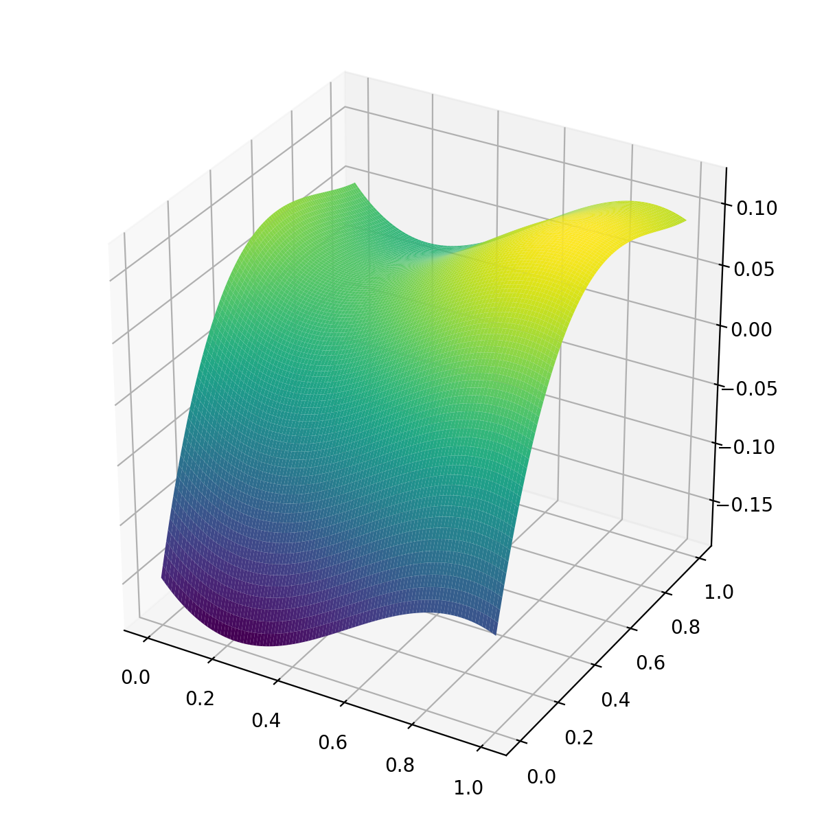
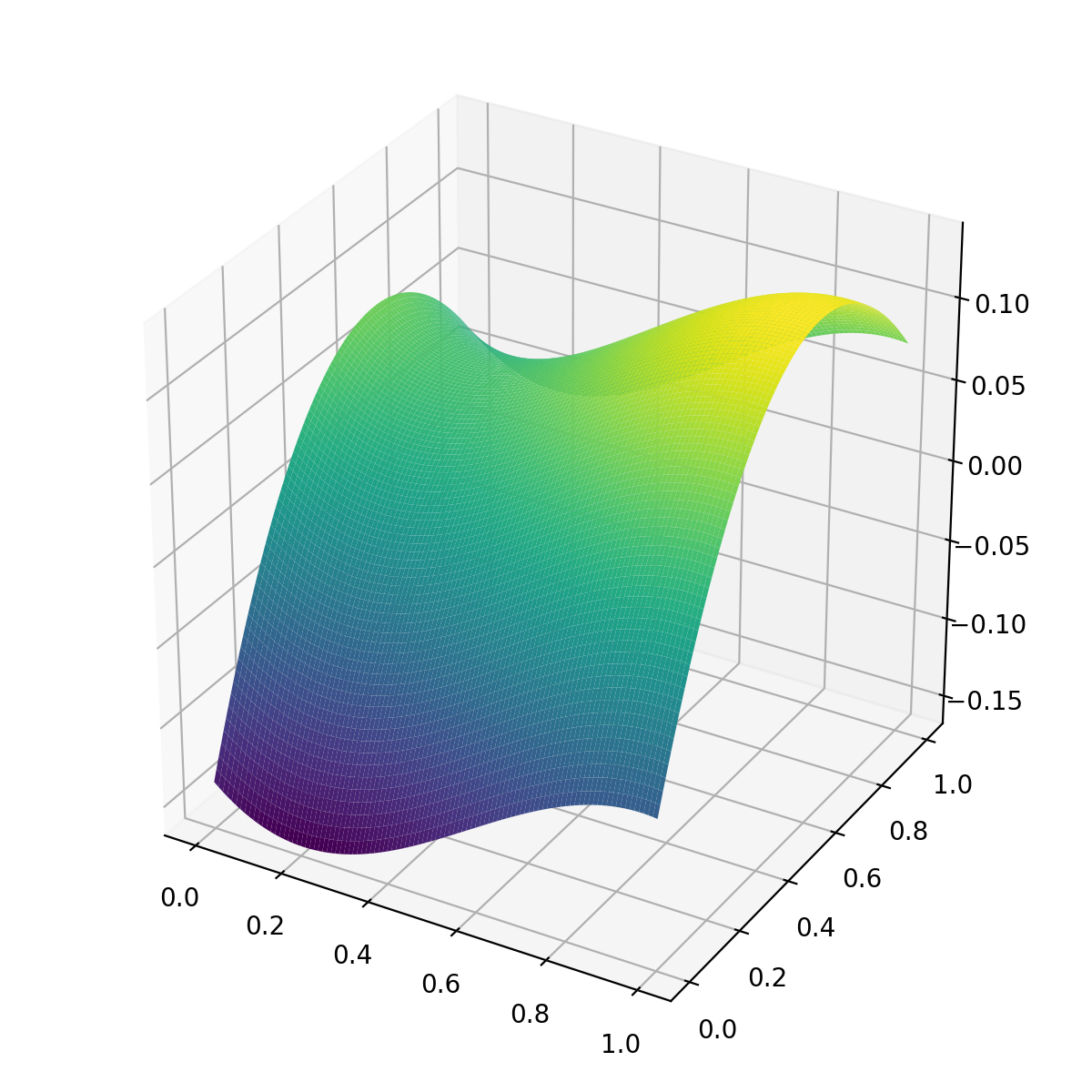
Figure 1: (Left) $g_{1,1}^{\star}(\mathbf{x})$ generated under additive model. (Right) $\widehat{g}_{1,1}(\mathbf{x})$ estimated under additive assumption.

Further, we simulate the data such that the additive assumption (7) is not valid. Specifically, we generate $g_{m,r_{m}}(\mathbf{x}_{m,i_{m}\cdot})$ in a multiplicative scheme such that

$$g_{m,r_{m}}(\mathbf{x}_{m,i_{m}\cdot})=\prod_{d_{m}=1}^{D_{m}}g_{m,r_{m},d_{m}}(x_{m,i_{m}d_{m}}).$$ (13)

where $g_{m,r_{m},d_{m}}$ remains the sieve structure (12). We conduct the IP-SVD procedure using the additive approximation (7). The true and estimated function of $g_{1,1}(\mathbf{x})$ are plotted in Figure 2(a) and 2(c), respectively. The estimated function can capture some structures of the true function but misses other details as we approximate it with the additive form. Figure 2(b) depicts the projection of the true functin $g_{1,1}^{\star}$ to the additive sieve space used in IP-SVD. The projection is supposed to be the best function estimate that can be obtained from the additive sieve basis. Note that, as mentioned in previous sections, $\mathbf{A}$ is identified up to an orthogonal matrix, so is $\mathbf{G}$. To address this potential unidentifiability problem of $g_{1,1}$, we calculate the best linear combination of $\widehat{g}_{1,r}$, $r=1,\dots,R$, that is closest to $g_{1,1}^{*}$ to mimic any potential orthogonal matrix applied to $\mathbf{G}$. The best linear combination is reported in Figure 2(d). As one can see, Figure 2(b) and Figure 2(d) are almost identical to each other. In conclusion, the projected Tucker under an additive basis assumption can ideally recover at most the linear (and additive) part of the true parametric component $\mathbf{G}_{m}$. The performance of such an approximation depends on the deviation between the $\mathbf{G}_{m}$ and its projected version $\mathbf{P}_{m}\mathbf{G}_{m}$.

To assess the performance of IP-SVD when the additive assumption (7) becomes invalid, we repeat the experiment in Table 1 with exactly same settings except that the multiplicative scheme in (13) is used to generate $\mathbf{G}_{m}$. The errors in estimating $\mathbf{A}_{m}$ and ${\cal Y}$ are reported in Table 5. Comparing Table 1 with Table 5, we observe that even when the additive assumption in (7) is not valid, IP-SVD still performs better than HOOI. But the improvement under misspecification is not as good as that under the valid additive assumption. This shows empirically that even when the additive assumption is violated, IP-SVD in general performances better than HOOI as long as the sieve basis used in IP-SVD can partially explain the parametric part of $\mathbf{A}_{m}$ with respect to $\mathbf{X}_{m}$.

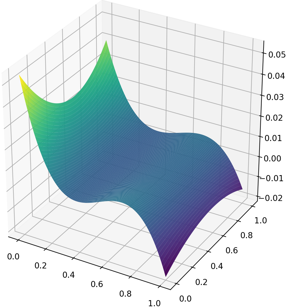
(a) $g_{1,1}^{\star}(\mathbf{x})$

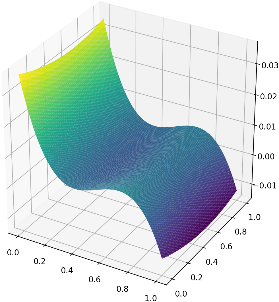
(b) $\mathbf{P}_{1}g_{1,1}(\mathbf{x})$

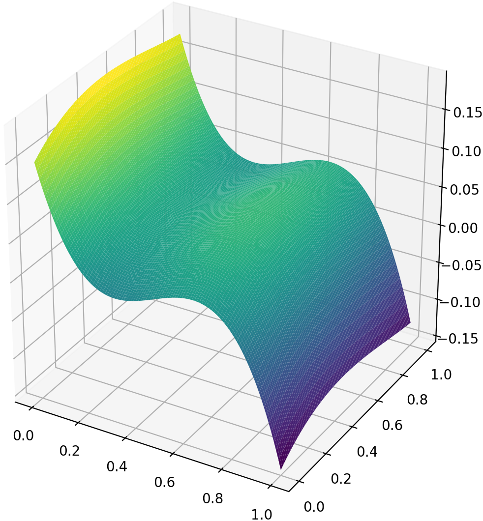
(c) $\widehat{g}_{1,1}(\mathbf{x})$

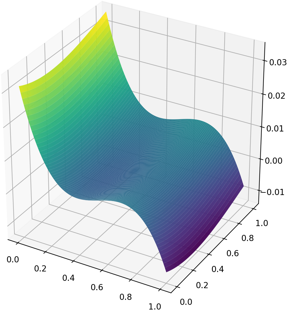
(d) $\sum_{r=1}^{R}a_{r}\widehat{g}_{1,r}(\mathbf{x})$

Figure 2: (a) True function of $g_{1,1}^{\star}(\mathbf{x})$ (b) Projected version of $g_{1,1}^{\star}(\mathbf{x})$ (c) Estimated $g_{1,1}(\mathbf{x})$ (d) Best linear combination of $\widehat{g}_{1,r}(\mathbf{x})$.

Table 5: Under varying dimensions and signal noise ratio. The mean and standard deviation of the the average Schatten q-$\sin\theta$ loss $\ell_{2}(\widehat{}\mathbf{A}_{1})$, from $100$ replications when the additive loading assumption is replaced with the multiplicative assumption.

	$\alpha$	0.1			0.3			0.5
	$I$	100	200	300	100	200	300	100	200	300
IP-SVD	$\ell_{2}(\widehat{}\mathbf{A}_{1})$	1.430 (0.103)	1.450 (0.126)	1.438 (0.115)	1.225 (0.165)	1.182 (0.210)	1.132 (0.203)	0.853 (0.212)	0.796 (0.217)	0.820 (0.228)
	${\rm ReMSE}_{{\cal Y}}$	2.596 (0.521)	2.395 (0.579)	2.375 (0.482)	1.189 (0.210)	1.095 (0.175)	0.984 (0.157)	0.741 (0.117)	0.709 (0.117)	0.704 (0.132)
HOOI	$\ell_{2}(\widehat{}\mathbf{A}_{1})$	1.705 (0.012)	1.720 (0.006)	1.723 (0.005)	1.705 (0.012)	1.720 (0.005)	1.724 (0.004)	1.568 (0.213)	1.653 (0.168)	1.663 (0.188)
	${\rm ReMSE}_{{\cal Y}}$	8.092 (1.686)	10.108 (2.596)	12.049 (2.701)	3.263 (0.672)	3.874 (0.721)	3.911 (0.781)	1.528 (0.332)	1.538 (0.294)	1.513 (0.300)

7 Real data applications

7.1 Multi-variate Spatial-Temporal Data

In this section, we illustrate the usefulness of the STEFA model and the IP-SVD algorithm on the Comprehensive Climate Dataset (CCDS) – a collection of climate records of North America. The dataset was compiled from five federal agencies sources by Lozano et al. (2009). Specifically, we show that we can use the STEFA and IP-SVD to estimate interpretable loading functions, deal better with large noises and make more accurate predictions than the vanilla Tucker decomposition.

The data contains monthly observations of 17 climate variables spanning from 1990 to 2001 on a $2.5\times 2.5$ degree grid for latitudes in $(30.475,50.475)$, and longitudes in $(-119.75,-79.75)$. The total number of observation locations is 125 and the whole time series spans from January, 1990 to December, 2001. Due to the data quality, we use only 16 measurements listed in Table 6 at each location and time point. Thus, the dimensions our our dataset are 125 (locations) $\times$ 16 (variables) $\times$ 156 (time points). Detailed information about data is given in Lozano et al. (2009).

Table 6: Variables and data sources in the Comprehensive Climate Dataset (CCDS)

Variables (Short name)	Variable group	Type	Source
Methane (CH4)	$CH_{4}$	Greenhouse Gases	NOAA
Carbon-Dioxide (CO2)	$CO_{2}$
Hydrogen (H2)	$H_{2}$
Carbon-Monoxide (CO)	$CO$
Temperature (TMP)	TMP	Climate	CRU
Temp Min (TMN)	TMP
Temp Max (TMX)	TMP
Precipitation (PRE)	PRE
Vapor (VAP)	VAP
Cloud Cover (CLD)	CLD
Wet Days (WET)	WET
Frost Days (FRS)	FRS
Global Horizontal (GLO)	SOL	Solar Radiation	NCDC
Direct Normal (DIR)	SOL
Global Extraterrestrial (ETR)	SOL
Direct Extraterrestrial (ETRN)	SOL

For a clear presentation, we focus on the spatial function structure of this data set although the temporal dimension can also incorporate a time covariate. The covariates $\mathbf{X}\in\mathbb{R}^{125\times 2}$ of the spacial dimension contain the latitudes and longitudes of all sampling locations, which basically capture the spatial continuity of factor loadings on mode 1. The semi-parametric form (4) for this application is written as

$${\cal Y}={\cal F}\times_{1}\left(\boldsymbol{\Phi}(\mathbf{X})\mathbf{B}+\mathbf{R}(\mathbf{X})+\boldsymbol{\Gamma}\right)\times_{2}\mathbf{A}_{2}\times_{3}\mathbf{I}+{\cal E}.$$ (14)

The first mode is the space dimension with loading matrix $\mathbf{A}_{1}=\boldsymbol{\Phi}(\mathbf{X})\mathbf{B}+\mathbf{R}(\mathbf{X})+\boldsymbol{\Gamma}$. The second mode is the variable dimension with $\mathbf{A}_{2}$ as the variable loading matrix. The third mode is the time dimension which we do not compress. So we use the identity matrix $\mathbf{I}$ in place of $\mathbf{A}_{3}$. This is a matrix-variate factor model similar to Chen, Fan and Li (2020) but incorporates covariate effects on the loading matrix in the spatial-mode. We normalized each time series to have a unit $\ell_{2}$ norm.

7.1.1 Estimating loading functions

We use $R_{1},R_{2},R_{3}=6,6,156$ where the time mode is not compressed and the other two latent dimensions are chosen according to the literature (Lozano et al., 2009; Bahadori, Yu and Liu, 2014; Chen et al., 2020a). We use the Legendre basis functions of order 5 for $\boldsymbol{\Phi}(\mathbf{X})$. Here we have $J=11$. Six estimated bi-variate loading functions corresponding to the six columns of $\boldsymbol{\Phi}(\mathbf{X})\widehat{}\mathbf{B}$ are plotted in Figure 3. The singular values corresponding to each column of $\boldsymbol{\Phi}(\mathbf{X})\widehat{}\mathbf{B}$ are $40.55$, $15.57$, $5.44$, $3.41$, $2.50$, and $2.26$. Or equivalently, the first to the sixth column of $\boldsymbol{\Phi}(\mathbf{X})\widehat{}\mathbf{B}$ explains approximately $84.79\%$ , $12.50\%$, $1.52\%$, $0.60\%$, $0.32\%$, $0.26\%$ of the variance along the first mode of the tensor after projection ${\cal Y}\times_{1}\mathbf{P}_{1}$. The space loading surfaces are highly nonlinear.

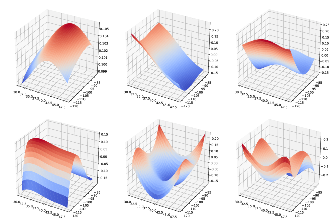
Figure 3: Estimated space loading surfaces $\widehat{}\mathbf{G}(\mathbf{X})=\boldsymbol{\Phi}(\mathbf{X})\widehat{}\mathbf{B}$. From the top-left to the bottom right sub-figures correspond to the first to the sixth space loading functions in order, with singular value $40.55$ ($84.79\%$), $15.57$ ($12.50\%$), $5.44$ ($1.52\%$), $3.41$ ($0.60\%$), $2.50$ ($0.32\%$), and $2.26$ ($0.26\%$), respectively. The space loading surfaces are highly nonlinear.

7.1.2 Fitting real data with amplified noise

In this section, we compare the vanilla and projected Tucker decomposition by their performances in fitting signal with different levels of noise. To generate different noise levels, we treat the estimated signal $\widehat{\cal S}_{v}$ and noise $\widehat{\cal E}_{v}$ from vanilla Tucker decomposition as the true signal ${\cal S}$ and noise ${\cal E}$ and calibrate the real data with different noise amplifier $\alpha>0$. Specifically, the calibrated data is generated as

$${\cal Y}=\widehat{\cal S}_{v}+\alpha\times\widehat{\cal E}_{v}.$$

The setting $\alpha=1$ corresponds to the original data. We compare the relative mean square errors (ReMSE) of the signal estimator ${\left\lVert{\cal S}-\widehat{\cal S}\right\rVert^{2}_{F}}/{\left\lVert{\cal S}\right\rVert^{2}_{F}}$ for vanilla and projected Tucker decomposition in Figure 4. For the projected Tucker decomposition, we report two estimators based on estimated loading matrix $\widehat{}\mathbf{A}_{1}=\boldsymbol{\Phi}(\mathbf{X})\widehat{}\mathbf{B}+\widehat{}\mathbf{R}(\mathbf{X})+\widehat{}\boldsymbol{\Gamma}$ and on only space loading function $\widehat{}\boldsymbol{\Phi}(X)\mathbf{B}$. Two methods behave the same in the noiseless case where $\alpha=0$. When $\alpha=1$ (original data) three methods perform similarly. When $\alpha\in(0,1)$ vanilla Tucker decomposition performs the best. This makes sense because we treat $\widehat{\cal S}_{v}$ estimated by vanilla Tucker decomposition as the true signal. The noise term $\alpha\cdot\widehat{\cal E}_{v}$ is reduced when $\alpha\in(0,1)$. When $\alpha>1$, however, vanilla Tucker decomposition performs the worst even though data is generated using $\widehat{\cal S}_{v}$ as the truth. This shows that the projected Tucker decomposition is more stable in the low SNR case.

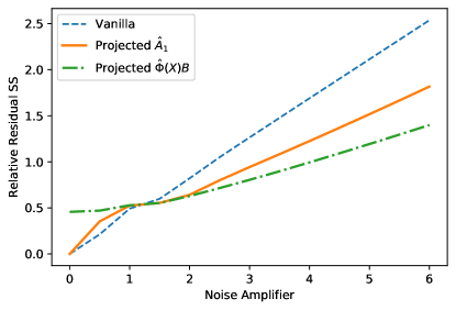
Figure 4: Relative mean square errors (ReMSE) by projected versus vanilla Tucker projections with different noise amplifiers. The relative residual SS of the signal part is defined as ${\left\lVert{\cal S}-\widehat{\cal S}\right\rVert^{2}_{F}}/{\left\lVert{\cal S}\right\rVert^{2}_{F}}$. Projected $\widehat{}\mathbf{A}_{1}=\boldsymbol{\Phi}(\mathbf{X})\widehat{}\mathbf{B}+\widehat{}\mathbf{R}(\mathbf{X})+\widehat{}\boldsymbol{\Gamma}$ corresponds to the estimated signal $\widehat{\cal S}\triangleq\widehat{\cal F}\times_{1}\widehat{}\mathbf{A}_{1}\times_{2}\widehat{}\mathbf{A}_{2}$. Projected $\widehat{}\boldsymbol{\Phi}(\mathbf{X})\mathbf{B}$ corresponds to the estimated signal $\widehat{\cal S}\triangleq\widehat{\cal F}\times_{1}\widehat{}\boldsymbol{\Phi}(\mathbf{X})\widehat{}\mathbf{B}\times_{2}\widehat{}\mathbf{A}_{2}$

7.1.3 Spatial prediction

In this section, we compare the prediction performances of the methods based vanilla and projected Tucker decomposition. The two prediction procedures are presented in Section 4. We randomly choose the training set to be $50\%$, $33\%$, and $25\%$ of the whole data set. Table 7 shows the prediction errors, average over cross validations, of the two methods respectively. It is clear that the STEFA model with projected Tucker decomposition outperforms the vanilla methods.

Table 7: Relative prediction error (averaged value by cross validation). For ease of display, the errors for Vanilla and Projected Tucker are reported in true value $\times 100$.

Training set ratio	$50\%$	$67\%$	$85\%$
Vanilla	3.52	3.48	3.04
Projected	3.24	3.25	3.04
Improvement	8%	7%	0%

7.2 Dynamic Networks with Covariates

In this section, we illustrate the versatility of the proposed framework with a complex real-world dynamic international trade flows. We use quarterly multilateral import and export volumes of commodity goods among 19 countries and regions over the 1981 – 2015 period. The data come from the International Monetary Fund (IMF) Direction of Trade Statistics (DOTS) (IMF, 2017), which provides monthly data on countries’ exports and imports with their partners. The source has been widely used in international trade analysis such as the Bloomberg Trade Flow. The countries and regions used in alphabetic order are Australia, Canada, China Mainland, Denmark, Finland, France, Germany, Indonesia, Ireland, Italy, Japan, Korea, Mexico, Netherlands, New Zealand, Spain, Sweden, United Kingdom, and United States. The covariate is the the Gross Domestic Product (GDP) for the same 140 quarters collected from OECD. The proportion of missing data is $2.58\%$ in the OECD covariates subset and $0.34\%$ in the DOTS dynamic network subset that we used here. For missing data, we use forward or backward filling for data missing at the starting or ending time points and use cubic spline interpolation for those at the interior time points. Data are normalized to have mean zero and variance one for each time series.

There may exist structural changes over the entire 35 years. Since our main purpose is to illustrate the application of the proposed STEFA and projected Tucker decomposition in a complex real-world application, we do not employ a sophisticated structural change analysis here. Instead we simply divide the entire period into $7$ disjoint periods of $5$-year (i.e. $1981.Q1-1985.Q4$, $1986.Q1-1990.Q4$ and so forth) and assume that the loadings are constant within each $5$-year period. For each $5$-year period, we estimate a specific form of Model (5) with

$$\mathbf{A}_{1}=\mathbf{G}_{1}\left(\mathbf{X}\right)+\boldsymbol{\Gamma}_{1},\quad\mathbf{A}_{2}=\mathbf{G}_{2}\left(\mathbf{X}\right)+\boldsymbol{\Gamma}_{2},\quad\text{and }\mathbf{A}_{3}=\mathbf{I}_{3}.$$

The covaraites $\mathbf{X}\in\mathbb{R}$ are the average normalized GDP during the $5$-year window. Thus for each data analyzing window, the dynamic network flows constitute a order-3 tensor ${\cal Y}$ with dimensions $19\times 19\times 20$. To avoid over-fitting with 19 countries, we only fit a linear functions for each column of $\mathbf{G}_{1\cdot}(\cdot)$ and $\mathbf{G}_{2\cdot}(\cdot)$. Thus, the purpose of this example is to investigate the relationship between a country’s import/export and the GDP’s of its trading partners, rather than dimension reduction. For a selective of four representative countries, Figure 5 (Figure 6) present the standardized average volume of the imports (exports) of United States, China, France, and Australia from (to) a country with a specific standardized GDP. Particularly, Figure 5 plots the $\widehat{\cal F}\times_{1}\widehat{}\mathbf{G}_{1}(\mathbf{X})\times_{2}\mathbf{A}_{country,2}\times\mathbf{I}_{3}$ for $\mathbf{X}\in[-1,1]$ for $country=USA$, $CHN$, $FRA$, and $AUS$. Figure 6 plots $\widehat{\cal F}\times_{1}\widehat{}\mathbf{A}_{country,1}\times_{2}\widehat{}\mathbf{G}_{1}(\mathbf{X})\times\mathbf{I}_{3}$ for $\mathbf{X}\in[-1,1]$ for $country=USA$, $CHN$, $FRA$, and $AUS$. These four countries are representative of the $19$ countries we have in the data set.

Intuitively, people would think that a country will import more from countries with higher GDP and export more to countries with lower GDP. However, Figure 5 and 6 show that the relationship depends on countries and time. For example, as shown in the top-left plot in Figure 5: from 1981 to 1990 United States import more from countries with higher GDP (positive slope); but from 1991 to 2000 United States import more from countries with lower GDP; and the pattern is changing with the time. The pattern is also different cross countries. For example, China’s volumes of import and export do not vary a lot across countries with different GDP’s as shown by the nearly flat lines in the upper right plots of both figures.

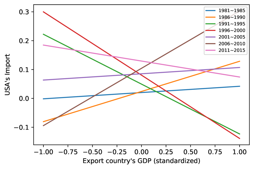
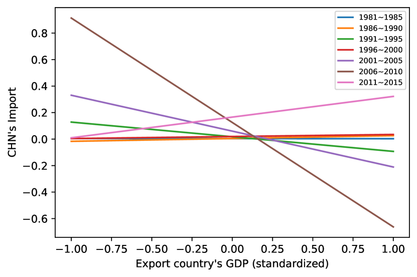
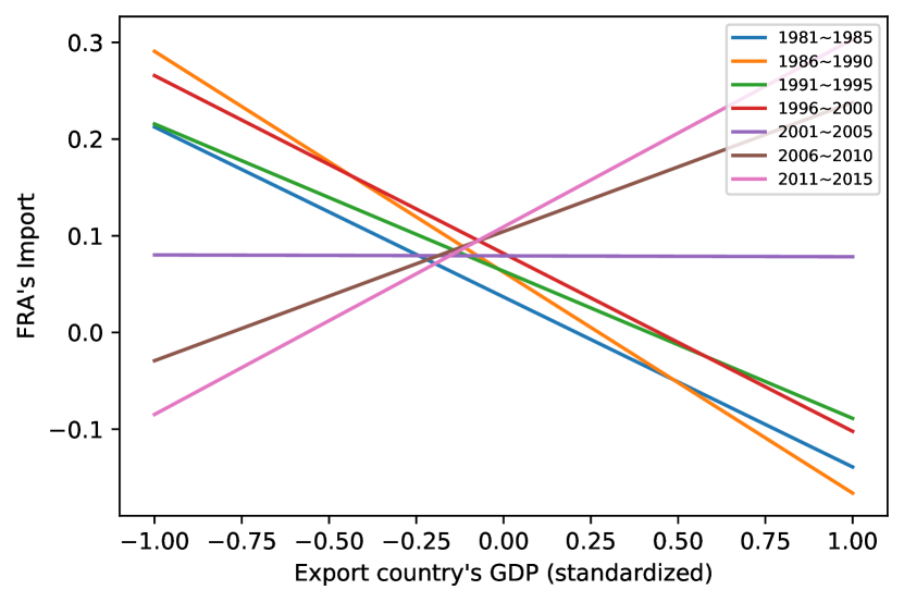
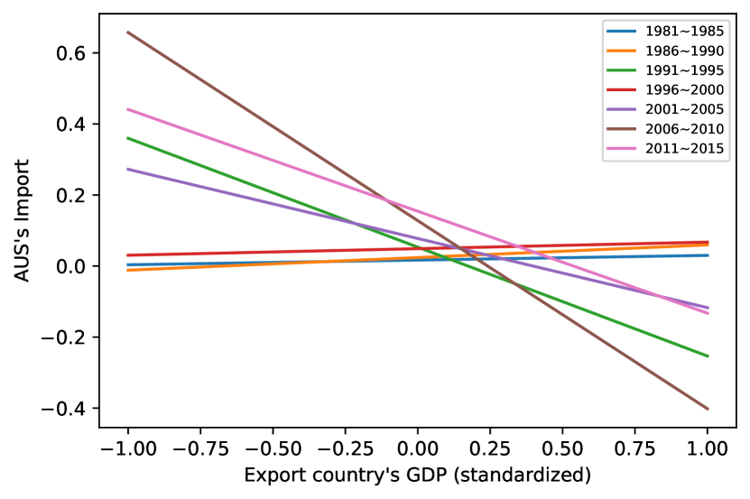
Figure 5: Countries’ import volumes (standardized) versus the GDP (standardized) of the trading counterpart.

Figure 6: Countries’ export volumes (standardized) versus the GDP (standardized) of the trading counterpart.

8 Discussion

This paper introduces a high-dimensional Semiparametric TEnsor FActor (STEFA) model with nonparametric loading functions that depend on a few observed covariates. This model is motivated by the fact that observed variables can explain partially the factor loadings, which helps to increase the accuracy of estimation and the interpretability of results. We propose a computationally efficient algorithm IP-SVD to estimate the unknown tensor factor, loadings, and the latent dimensions. The advantages of IP-SVD are two-fold. First, unlike HOOI which iterates in the ambient dimension, IP-SVD finds the principal components in the covariate-related subspace whose dimension can be significantly smaller. As a result, IP-SVD requires weaker SNR conditions for convergence. Secondly, the projection also reduces the effect dimension size of stochastic noise and thus IP-SVD yields an estimate of latent factors with faster convergence rates.

While tensor data is everywhere in the physical world, statistical analysis for tensor data is still challenging. There are several interesting topics for future researches. First, it is important to develop non-parametric tests on whether observed relevant covariates have explaining powers on the loadings and whether they fully explain the loadings. However, under the tensor decomposition setting, this is more challenging than a straightforward extension from Fan, Liao and Wang (2016). Second, we mentioned briefly that, when there are multiple observations, one can apply IP-SVD on the sample covariance tensor. However, a more precise algorithm is needed. Last but not the least, it is of great need to develop new methods to use STEFA in tensor regression or other tensor data related applications.

TECHNICAL PROOFS [doi] Supplement to STEFA-IPSVD.pdf We provide proofs for the theoretical results on the STEFA model and IP-SVD algorithm.

, , , and

University of California, Berkeley^∗, Hong Kong University of Science and Technology^†,
Temple University^§, Princeton University^‡

Supplement A: Proofs

Proof of Lemma 2.1.

Let ${\cal S}=\widetilde{\cal F}\times_{1}\widetilde{}\mathbf{A}_{1}\times_{2}\cdots\times_{M}\widetilde{}\mathbf{A}_{M}$ be a Tucker decomposition of ${\cal S}$ such that $\widetilde{\cal F}\in\mathbb{R}^{R_{1}\times\cdots\times R_{M}}$ is the core tensor, and for $m\in[M]$, $\widetilde{}\mathbf{A}_{m}\in\mathbb{R}^{I_{m}\times R_{m}}$ is the $m$-mode loading matrix satisfying Assumption 1(a).

Clearly, ${\cal S}={\cal F}\times_{1}\mathbf{A}_{1}\times_{2}\cdots\times_{M}\mathbf{A}_{M}$ is a valid Tucker decomposition satisfying Assumption 1(a) if and only if there exist orthogonal matrices $\mathbf{H}_{m}\in\mathbb{O}^{R_{m}\times R_{m}}$ for all $m\in[M]$ such that $\mathbf{A}_{m}=\widetilde{}\mathbf{A}_{m}\mathbf{H}_{m}$ and ${\cal F}=\widetilde{\cal F}\times_{1}\mathbf{H}_{1}^{\top}\times_{2}\cdots\times_{m}\mathbf{H}_{M}^{\top}$. Moreover, then ${\cal M}_{m}({\cal S}){\cal M}_{m}({\cal S})^{\top}/I_{m}$ has the same singular values with ${\cal M}_{m}({\cal F}){\cal M}_{m}({\cal F})^{\top}$

Now we are in the place to prove the lemma. Recall that any Tucker decomposition of ${\cal S}$ satisfying Assumption 1(a) are indexed by the set of orthogonal matrices $(\mathbf{H}_{1},\cdots,\mathbf{H}_{M})$ in reference to the decomposition ${\cal S}=\widetilde{\cal F}\times_{1}\widetilde{}\mathbf{A}_{1}\times_{2}\cdots\times_{M}\widetilde{}\mathbf{A}_{M}$. The corresponding core tensor ${\cal F}$ is ${\cal F}=\widetilde{\cal F}\times_{1}\mathbf{H}_{1}^{\top}\times_{2}\cdots\times_{M}\mathbf{H}_{M}^{\top}$. The mode-$m$ matricization of ${\cal F}$ is ${\cal M}_{m}({\cal F})=\mathbf{H}_{m}^{\top}{\cal M}_{m}(\widetilde{\cal F})\left[\bigotimes_{l\in[M],l\neq m}\mathbf{H}_{l}^{\top}\right]$. Suppose for some $\mathbf{H}_{m}$, Assumption 1(a) is satisfied such that ${\cal M}_{m}({\cal F}){\cal M}_{m}({\cal F})^{\top}=\mathbf{H}_{m}^{\top}{\cal M}_{m}(\widetilde{\cal F}){\cal M}_{m}(\widetilde{\cal F})^{\top}\mathbf{H}_{m}=\mathbf{D}_{m}$ for some diagonal matrix $\mathbf{D}_{m}$ with non-zero decreasing diagonal entries. Then the diagonal entries of $\mathbf{D}_{m}$ are the eigenvalues of ${\cal M}_{m}(\widetilde{\cal F}){\cal M}_{m}(\widetilde{\cal F})^{\top}$ and the columns in $\mathbf{H}_{m}$ are the corresponding eigenvectors, because of the equality ${\cal M}_{m}(\widetilde{\cal F}){\cal M}_{m}(\widetilde{\cal F})^{\top}\mathbf{H}_{m}=\mathbf{H}_{m}\mathbf{D}_{m}$. Note that $\mathbf{D}_{m}$ has the same singular values with ${\cal M}_{m}({\cal S}){\cal M}_{m}({\cal S})^{\top}$. As a result, when the singular values of ${\cal M}_{m}({\cal S}){\cal M}_{m}({\cal S})^{\top}$ are distinct, the eigenvalues and eigenvectors of ${\cal M}_{m}(\widetilde{\cal F}){\cal M}_{m}(\widetilde{\cal F})^{\top}$ can be uniquely identified (up to a global sign), resulting in an unique $\mathbf{H}_{m}$. Here, the uniqueness is up to a column-wise sign of $\mathbf{H}_{m}$.

In conclusion, starting from an arbitrary Tucker decomposition ${\cal S}=\widetilde{\cal F}\times_{1}\widetilde{}\mathbf{A}_{1}\times_{2}\cdots\times_{M}\widetilde{}\mathbf{A}_{M}$ satisfying Assumption 1(a), by choosing the columns of $\mathbf{H}_{m}$ to be the eigenvectors of ${\cal M}_{m}(\widetilde{\cal F}){\cal M}_{m}(\widetilde{\cal F})^{\top}$ in descending order of eigenvalues, the Tucker decomposition with ${\cal F}=\widetilde{\cal F}\times_{1}\mathbf{H}_{1}^{\top}\times_{2}\cdots\times_{M}\mathbf{H}_{M}^{\top},\mathbf{A}_{1}=\widetilde{}\mathbf{A}_{1}\mathbf{H}_{1},\cdots,\mathbf{A}_{M}=\widetilde{}\mathbf{A}_{M}\mathbf{H}_{M}$ is the unique Tucker decomposition satisfying both Assumptions 1(a) and 1(b) when the eigenvalues of ${\cal M}_{m}({\cal S}){\cal M}_{m}({\cal S})^{\top}$ are distinct for all $m\in[M]$. ∎

Proof of Lemma 5.1.

We prove the initialization error and convergence of IP-SVD separately.

We begin with the upper bound of the remainder term $\mathbf{R}_{m}(\mathbf{X}_{m})$. By Assumption 3, for each function $m\in[M]$ and $1\leq r_{m}\leq R_{m}$, $|g_{m,r_{m}}(\mathbf{x}_{i_{m}})-\mathbf{b}_{m,r_{m}}^{\top}\boldsymbol{\phi}_{m}(\mathbf{x}_{i_{m}})|=O(J_{m}^{-\tau/2})$ which bounds the $(i_{m},r_{m})$-th entry of $\mathbf{R}_{m}(\mathbf{X}_{m})$. Therefore, a simple fact is

$$\|\mathbf{R}_{m}(\mathbf{X}_{m})\|_{\rm F}^{2}/I_{m}=O\big{(}R_{m}\cdot J_{m}^{-\tau}\big{)}$$ (15)

for all $m\in[M]$.

Initialization error. Without loss of generality, we assume that $\mathbb{E}\varepsilon_{i_{1},i_{2},i_{3}}^{2}=1$ and only prove the upper bound of $\|\widetilde{}\mathbf{G}_{1}^{(0)}\widetilde{}\mathbf{G}_{1}^{(0)\top}-\mathbf{G}_{1}\mathbf{G}_{1}^{\top}\|_{\rm F}$. Recall that $\mathbf{G}_{1}=\boldsymbol{\Phi}_{1}(\mathbf{X}_{1})\mathbf{B}_{1}+\mathbf{R}_{1}(\mathbf{X}_{1})$ where, by the definition of $\boldsymbol{\Phi}_{1}(\mathbf{X}_{1})$, we have $\boldsymbol{\Phi}_{1}(\mathbf{X}_{1})^{\top}\boldsymbol{\Gamma}_{1}={\bf 0}$. Let $\check{\mathbf{G}}_{1}/\sqrt{I_{1}}$ denotes the top-$R_{1}$ left singular vectors of $\boldsymbol{\Phi}_{1}(\mathbf{X}_{1})\mathbf{B}_{1}$. By Condition (15) and Davis-Kahan theorem (Davis and Kahan, 1970) or spectral perturbation formula (Xia, 2019),

$$\|\check{\mathbf{G}}_{1}\check{\mathbf{G}}_{1}^{\top}-\mathbf{G}_{1}\mathbf{G}_{1}^{\top}\|_{\rm F}/I_{1}=O\big{(}\sqrt{R_{1}}\cdot J_{1}^{-\tau/2}\big{)}$$

where we used the fact that $\sigma_{R_{1}}\big{(}\boldsymbol{\Phi}_{1}(\mathbf{X}_{1})\mathbf{B}_{1}/\sqrt{I_{1}}\big{)}\geq 1-O(\sqrt{R_{1}}\cdot J_{1}^{-\tau/2})\geq 1/2$ and $\|\mathbf{R}_{1}(\mathbf{X}_{1})\|_{\rm F}/\sqrt{I_{1}}=O(\sqrt{R_{1}}\cdot J_{1}^{-\tau/2})$.

Recall that $\widetilde{\cal Y}={\cal F}\times_{1}(\mathbf{P}_{1}\mathbf{G}_{1})\times_{2}(\mathbf{P}_{2}\mathbf{G}_{2})\times_{3}(\mathbf{P}_{3}\mathbf{G}_{3})+{\cal E}\times_{1}\mathbf{P}_{1}\times_{2}\mathbf{P}_{2}\times_{3}\mathbf{P}_{3}$ and as a result

$${\cal M}_{1}(\widetilde{\cal Y})=\mathbf{P}_{1}\mathbf{G}_{1}{\cal M}_{1}({\cal F})\big{(}(\mathbf{P}_{2}\mathbf{G}_{2})\odot(\mathbf{P}_{3}\mathbf{G}_{3})\big{)}^{\top}+\mathbf{P}_{1}{\cal M}_{1}({\cal E})(\mathbf{P}_{2}\odot\mathbf{P}_{3})^{\top}$$

where we denote $\odot$ the kronecker product. The projector matrix $\mathbf{P}_{m}\in\mathbb{R}^{I_{m}\times I_{m}}$ with $\operatorname{rank}(\mathbf{P}_{m})=J_{m}$. Denote the eigen-decomposition of $\mathbf{P}_{m}$ by $\mathbf{P}_{m}=\mathbf{U}_{m}\mathbf{U}_{m}^{\top}\ {\rm where}\ \mathbf{U}_{m}^{\top}\mathbf{U}_{m}=\mathbf{I}_{J_{m}}.$ Therefore, we write

$$\mathbf{P}_{1}{\cal M}_{1}({\cal E})(\mathbf{P}_{2}\odot\mathbf{P}_{3})=\mathbf{U}_{1}\big{(}\mathbf{U}_{1}^{\top}{\cal M}_{1}({\cal E})(\mathbf{U}_{2}\odot\mathbf{U}_{3})\big{)}(\mathbf{U}_{2}\odot\mathbf{U}_{3})^{\top}.$$

In addition, we write

$$\mathbf{P}_{1}\mathbf{G}_{1}{\cal M}_{1}({\cal F})\big{(}(\mathbf{P}_{2}\mathbf{G}_{2})\odot(\mathbf{P}_{3}\mathbf{G}_{3})\big{)}^{\top}=\mathbf{P}_{1}\boldsymbol{\Phi}_{1}(\mathbf{X}_{1})\mathbf{B}_{1}{\cal M}_{1}({\cal F})\big{(}(\mathbf{P}_{2}\mathbf{G}_{2})\odot(\mathbf{P}_{3}\mathbf{G}_{3})\big{)}^{\top}$$

$$+\mathbf{P}_{1}\mathbf{R}_{1}(\mathbf{X}_{1}){\cal M}_{1}({\cal F})\big{(}(\mathbf{P}_{2}\mathbf{G}_{2})\odot(\mathbf{P}_{3}\mathbf{G}_{3})\big{)}^{\top}$$

where the left singular space of the first matrix is the same to column space of $\check{}\mathbf{G}_{1}$. Denote the top-$R_{1}$ left singular vectors of $\mathbf{P}_{1}\mathbf{G}_{1}{\cal M}_{1}({\cal F})\big{(}(\mathbf{P}_{2}\mathbf{G}_{2})\odot(\mathbf{P}_{3}\mathbf{G}_{3})\big{)}^{\top}$ by $\mathring{\mathbf{G}}_{1}/\sqrt{I_{1}}$. Again by Davis-Kahan theorem (Davis and Kahan, 1970) or spectral perturbation formula (Xia, 2019), we have

$$\|\mathring{\mathbf{G}}_{1}\mathring{\mathbf{G}}_{1}^{\top}-\check{\mathbf{G}}_{1}\check{\mathbf{G}}_{1}^{\top}\|_{\rm F}/I_{1}=O(\kappa_{0}\sqrt{R_{1}}\cdot J_{1}^{-\tau/2})$$

where $\kappa_{0}$ is ${\cal F}$’s condition number and we used the facts

$$\sigma_{R_{1}}\Big{(}\mathbf{P}_{1}\boldsymbol{\Phi}_{1}(\mathbf{X}_{1})\mathbf{B}_{1}{\cal M}_{1}({\cal F})\big{(}(\mathbf{P}_{2}\mathbf{G}_{2})\odot(\mathbf{P}_{3}\mathbf{G}_{3})\big{)}^{\top}\Big{)}\geq \lambda_{\min}\sqrt{I_{2}I_{3}}\cdot\sigma_{R_{1}}\big{(}\boldsymbol{\Phi}_{1}(\mathbf{X}_{1})\mathbf{B}_{1}\big{)}$$

$$\geq\lambda_{\min}\sqrt{I_{1}I_{2}I_{3}}/2$$

and

$$\Big{\|}\mathbf{P}_{1}\mathbf{R}_{1}(\mathbf{X}_{1}){\cal M}_{1}({\cal F})\big{(}(\mathbf{P}_{2}\mathbf{G}_{2})\odot(\mathbf{P}_{3}\mathbf{G}_{3})\big{)}^{\top}\Big{\|}_{\rm F}= O\big{(}\kappa_{0}\lambda_{\min}\sqrt{I_{2}I_{3}}\cdot\|\mathbf{R}_{1}(\mathbf{X}_{1})\|_{\rm F}\big{)}$$

$$=O(\kappa_{0}\lambda_{\min}\sqrt{R_{1}I_{1}I_{2}I_{3}}\cdot J_{1}^{-\tau/2}).$$

For notational simplicity, we write ${\cal M}_{1}(\widetilde{{\cal Y}})=\mathbf{A}_{1}+\mathbf{Z}_{1}$ where $\mathbf{A}_{1}=\mathbf{P}_{1}\mathbf{G}_{1}{\cal M}_{1}({\cal F})\big{(}(\mathbf{P}_{2}\mathbf{G}_{2})\odot(\mathbf{P}_{3}\mathbf{G}_{3})\big{)}^{\top}$ and $\mathbf{Z}_{1}=\mathbf{P}_{1}{\cal M}_{1}({\cal E})(\mathbf{P}_{2}\odot\mathbf{P}_{3})^{\top}$. Then, $\mathring{\mathbf{G}}_{1}/\sqrt{I_{1}}$ are the top-$R_{1}$ left singular vectors of $\mathbf{A}_{1}$ and are also the top-$R_{1}$ eigenvectors of $\mathbf{A}_{1}\mathbf{A}_{1}^{\top}$. Since $\widetilde{}\mathbf{G}_{1}^{(0)}/\sqrt{I_{1}}$ are the top-$R_{1}$ left singular vectors of ${\cal M}_{1}(\widetilde{{\cal Y}})$, they are also the top-$R_{1}$ eigenvectors of ${\cal M}_{1}(\widetilde{{\cal Y}}){\cal M}_{1}^{\top}(\widetilde{{\cal Y}})$ whcih can be written as ${\cal M}_{1}(\widetilde{{\cal Y}}){\cal M}_{1}^{\top}(\widetilde{{\cal Y}})=\mathbf{A}_{1}\mathbf{A}_{1}^{\top}+\mathbf{A}_{1}\mathbf{Z}_{1}^{\top}+\mathbf{Z}_{1}\mathbf{A}_{1}^{\top}+\mathbf{Z}_{1}\mathbf{Z}_{1}^{\top}.$ Observe that

$$\mathbf{Z}_{1}\mathbf{Z}_{1}^{\top}=\mathbf{U}_{1}\big{(}\mathbf{U}_{1}^{\top}{\cal M}_{1}({\cal E})(\mathbf{U}_{2}\odot\mathbf{U}_{3})\big{)}\big{(}\mathbf{U}_{1}^{\top}{\cal M}_{1}({\cal E})(\mathbf{U}_{2}\odot\mathbf{U}_{3})\big{)}^{\top}\mathbf{U}_{1}^{\top}.$$

Then, we can write

$${\cal M}_{1}(\widetilde{{\cal Y}}){\cal M}_{1}^{\top}(\widetilde{{\cal Y}})=\mathbf{A}_{1}\mathbf{A}_{1}^{\top}+J_{2}J_{3}\mathbf{P}_{1}+\mathbf{A}_{1}\mathbf{Z}_{1}^{\top}+\mathbf{Z}_{1}\mathbf{A}_{1}^{\top}+\mathbf{Z}_{1}\mathbf{Z}_{1}^{\top}-J_{2}J_{3}\mathbf{P}_{1}.$$

Recall that the column space of $\check{}\mathbf{G}_{1}$ is a subspace of the column space of $\mathbf{P}_{1}$. Denote ${\cal P}_{\check{\mathbf{G}}_{1}}=\check{\mathbf{G}}_{1}\check{\mathbf{G}}_{1}^{\top}/I_{1}$ and ${\cal P}_{\check{\mathbf{G}}_{1}}^{\perp}$ the projector onto the orthogonal space of $\check{\mathbf{G}}_{1}$. Then, write

$${\cal M}_{1}(\widetilde{{\cal Y}}){\cal M}_{1}^{\top}(\widetilde{{\cal Y}})=\underbrace{\big{(}{\cal P}_{\check{\mathbf{G}}_{1}}\mathbf{A}_{1}\mathbf{A}_{1}{\cal P}_{\check{\mathbf{G}}_{1}}+J_{2}J_{3}\mathbf{P}_{1}\big{)}}_{\mathbf{M}}+\underbrace{{\cal P}_{\check{\mathbf{G}}_{1}}^{\perp}\mathbf{A}_{1}\mathbf{A}_{1}+{\cal P}_{\check{\mathbf{G}}_{1}}\mathbf{A}_{1}\mathbf{A}_{1}{\cal P}_{\check{\mathbf{G}}_{1}}^{\perp}}_{{\cal R}_{\mathbf{A}_{1}}}$$

$$+(\mathbf{A}_{1}\mathbf{Z}_{1}^{\top}+\mathbf{Z}_{1}\mathbf{A}_{1}^{\top})+\mathbf{Z}_{1}\mathbf{Z}_{1}^{\top}-J_{2}J_{3}\mathbf{P}_{1}.$$

Clearly, the top-$R_{1}$ left singular space of $\mathbf{M}$ is the column space of $\check{\mathbf{G}}_{1}$ and $\sigma_{R_{1}}(\mathbf{M})-\sigma_{R_{1}+1}(\mathbf{M})\geq\lambda_{\min}^{2}(I_{1}I_{2}I_{3})/2$. Note that

$$\|{\cal P}_{\check{\mathbf{G}}_{1}}^{\perp}\mathbf{P}_{1}\mathbf{G}_{1}\|_{\rm F}= \|{\cal P}_{\check{\mathbf{G}}_{1}}^{\perp}\mathbf{G}_{1}\|_{\rm F}=\|\mathbf{G}_{1}-\check{\mathbf{G}}_{1}\check{\mathbf{G}}_{1}^{\top}\mathbf{G}_{1}/I_{1}\|_{\rm F}$$

$$= \|(\mathbf{G}_{1}\mathbf{G}_{1}^{\top}-\check{\mathbf{G}}_{1}\check{\mathbf{G}}_{1}^{\top})\mathbf{G}_{1}/I_{1}\|_{\rm F}\leq\|\mathbf{G}_{1}\mathbf{G}_{1}^{\top}-\check{\mathbf{G}}_{1}\check{\mathbf{G}}_{1}\|_{\rm F}/\sqrt{I_{1}}=O(\kappa_{0}\sqrt{I_{1}R_{1}}\cdot J_{1}^{-\tau/2})$$

which implies that $\|{\cal R}_{\mathbf{A}_{1}}\|_{\rm F}=O\big{(}\kappa_{0}^{2}\lambda_{\min}^{2}I_{1}I_{2}I_{3}\cdot\sqrt{R_{1}}J_{1}^{-\tau/2}\big{)}$.

By Lemma 14 in Xia and Zhou (2019), the following bound holds with probability at least $1-e^{-(J_{1}\vee\alpha)}$ for any $\alpha>0$

$$\|\mathbf{A}_{1}\mathbf{Z}_{1}^{\top}+\mathbf{Z}_{1}\mathbf{A}_{1}^{\top}\|=O_{p}\big{(}\kappa_{0}\lambda_{\min}\sqrt{I_{1}I_{2}I_{3}}\cdot\sqrt{J_{1}\vee(R_{2}R_{3})\vee\alpha}\big{)}$$

where we used the fact that $\mathbf{U}_{1}^{\top}{\cal M}_{1}({\cal E})(\mathbf{U}_{2}\odot\mathbf{U}_{3})$ is a $(J_{1})\times(J_{2}J_{3})$ matrix and each entry is a centered sub-Gaussian random variable with equal variances. Note that we assumed $R_{m}\leq J_{m}$. Observe that

$$\mathbf{Z}_{1}\mathbf{Z}_{1}^{\top} -J_{2}J_{3}\mathbf{P}_{1}$$

$$= \mathbf{U}_{1}\Big{(}\big{(}\mathbf{U}_{1}^{\top}{\cal M}_{1}({\cal E})(\mathbf{U}_{2}\odot\mathbf{U}_{3})\big{)}\big{(}\mathbf{U}_{1}^{\top}{\cal M}_{1}({\cal E})(\mathbf{U}_{2}\odot\mathbf{U}_{3})\big{)}^{\top}-J_{2}J_{3}\mathbf{I}_{J_{1}}\Big{)}\mathbf{U}_{1}^{\top}.$$

Similarly, as shown in Xia and Zhou (2019) (Lemma 14), with probability at least $1-e^{-(J_{1}\vee\alpha)}$ for any $\alpha>0$

$$\big{\|}\mathbf{Z}_{1}\mathbf{Z}_{1}^{\top}-J_{2}J_{3}\mathbf{P}_{1}\big{\|}=O\big{(}\big{(}(J_{1}\vee\alpha)J_{2}J_{3}\big{)}^{1/2}\big{)}.$$

By Davis-Kahan theorem (Davis and Kahan, 1970), we get

$$\|\check{}\mathbf{G}_{1}\check{}\mathbf{G}_{1}^{\top}-\widetilde{\mathbf{G}}_{1}^{(0)}\widetilde{\mathbf{G}}_{1}^{(0)\top}\|_{\rm F}/I_{1}=O\Big{(}\frac{\kappa_{0}\sqrt{R_{1}(J_{1}\vee(R_{2}R_{3})\vee\alpha)}}{\lambda_{\min}\sqrt{I_{1}I_{2}I_{3}}}+\frac{\big{(}R_{1}(J_{1}\vee t)J_{2}J_{3}\big{)}^{1/2}}{\lambda_{\min}^{2}I_{1}I_{2}I_{3}}+\kappa_{0}^{2}\sqrt{R_{1}}\cdot J_{1}^{-\tau/2}\Big{)}$$

which holds with probability at least $1-2e^{-(J_{1}\vee\alpha)}$. Note that we assumed $\lambda_{\min}\sqrt{I_{1}I_{2}I_{3}}\geq C_{1}\Big{(}\sqrt{\kappa_{0}^{2}(J_{1}\vee(R_{2}R_{3})\vee\alpha)}\bigvee\big{(}(J_{1}\vee\alpha)J_{2}J_{3}\big{)}^{1/4}\Big{)}$ for a large enough absolute constant $C_{1}>0$.

Together with the bound of $\|\check{\mathbf{G}}_{1}\check{\mathbf{G}}_{1}^{\top}-\mathbf{G}_{1}\mathbf{G}_{1}^{\top}\|_{\rm F}$. Therefore, we conclude that with probability at least $1-2e^{-(J_{1}\vee\alpha)}$

$$\|\widetilde{}\mathbf{G}_{1}^{(0)}\widetilde{}\mathbf{G}_{1}^{(0)\top}-\mathbf{G}_{1}\mathbf{G}_{1}^{\top}\|_{\rm F}/I_{1}=O\Big{(}\frac{\kappa_{0}\sqrt{R_{1}(J_{1}\vee(R_{2}R_{3})\vee\alpha)}}{\lambda_{\min}\sqrt{I_{1}I_{2}I_{3}}}+\frac{\big{(}R_{1}(J_{1}\vee\alpha)J_{2}J_{3}\big{)}^{1/2}}{\lambda_{\min}^{2}I_{1}I_{2}I_{3}}+\kappa_{0}^{2}\sqrt{R_{1}}\cdot J_{1}^{-\tau/2}\Big{)}.$$

The proof is completed by assuming $\kappa_{0}=O(1)$.

IP-SVD iterations. Without loss of generality, we fix an integer value of $t$ and prove the contraction inequality (11) for $m=1$. For notation simplicity, we denote

$${\rm Err}_{t}=\max_{m=1,2,3}\|\widetilde{}\mathbf{G}_{m}^{(t)}\widetilde{}\mathbf{G}_{m}^{(t)\top}-\mathbf{G}_{m}\mathbf{G}_{m}^{\top}\|_{\rm F}/I_{m}.$$

By projected power iteration in Section 3, the scaled singular vectors $\widetilde{}\mathbf{G}_{1}^{(t)}$ are obtained by

$$\widetilde{}\mathbf{G}_{1}^{(t)}/\sqrt{I_{1}}={\rm SVD}_{R_{1}}\Big{(}\mathbf{P}_{1}{\cal M}_{1}\Big{(}{\cal Y}\times_{2}\widetilde{}\mathbf{G}_{2}^{(t-1)\top}\times_{3}\widetilde{}\mathbf{G}_{3}^{(t-1)\top}\Big{)}\Big{)}$$

Recall $\mathbf{A}_{m}=\mathbf{G}_{m}+\boldsymbol{\Gamma}_{m}$ for $m=1,2,3$ and

$${\cal Y}=\underbrace{{\cal F}\times_{1}(\mathbf{G}_{1}+\boldsymbol{\Gamma}_{1})\times_{2}(\mathbf{G}_{2}+\boldsymbol{\Gamma}_{2})\times_{3}(\mathbf{G}_{3}+\boldsymbol{\Gamma}_{3})}_{{\cal S}}+{\cal E}.$$

We then write

$$\mathbf{P}_{1}{\cal M}_{1}\Big{(}{\cal Y}\times_{2}\widetilde{}\mathbf{G}_{2}^{(t-1)\top} \times_{3}\widetilde{}\mathbf{G}_{3}^{(t-1)\top}\Big{)}$$

$$= \mathbf{P}_{1}{\cal M}_{1}\Big{(}{\cal S}\times_{2}\widetilde{}\mathbf{G}_{2}^{(t-1)\top}\times_{3}\widetilde{}\mathbf{G}_{3}^{(t-1)\top}\Big{)}+\mathbf{P}_{1}{\cal M}_{1}\Big{(}{\cal E}\times_{2}\widetilde{}\mathbf{G}_{2}^{(t-1)\top}\times_{3}\widetilde{}\mathbf{G}_{3}^{(t-1)\top}\Big{)}.$$

By the fact $\mathbf{P}_{1}\boldsymbol{\Gamma}_{1}={\bf 0}$, we obtain

$$\mathbf{P}_{1}{\cal M}_{1}\Big{(}{\cal S}\times_{2}\widetilde{}\mathbf{G}_{2}^{(t-1)\top}\times_{3}\widetilde{}\mathbf{G}_{3}^{(t-1)\top}\Big{)}=\mathbf{P}_{1}\mathbf{G}_{1}{\cal M}_{1}({\cal F})\big{(}(\mathbf{A}_{2}^{\top}\widetilde{}\mathbf{G}_{2}^{(t-1)})\otimes(\mathbf{A}_{3}^{\top}\widetilde{}\mathbf{G}_{3}^{(t-1)})\big{)}.$$

Observe that $\mathbf{P}_{1}\mathbf{G}_{1}=\boldsymbol{\Phi}(\mathbf{X}_{1})\mathbf{B}_{1}+\mathbf{P}_{1}\mathbf{R}_{1}(\mathbf{X}_{1})$. By Condition (15), we get

$$\sigma_{\min}\big{(}\mathbf{P}_{1}\mathbf{G}_{1}/\sqrt{I_{1}}\big{)}\geq\sigma_{\min}\big{(}\boldsymbol{\Phi}_{1}(\mathbf{X}_{1})\mathbf{B}_{1}/\sqrt{I_{1}}\big{)}-O(\sqrt{R_{1}}\cdot J_{1}^{-\tau/2})\geq 1-O(\sqrt{R}_{1}\cdot J_{1}^{-\tau/2}).$$

Recall that the column space of $\widetilde{}\mathbf{G}_{m}^{(t-1)}$ is a subspace of $\boldsymbol{\Phi}_{m}(\mathbf{X}_{m})$ for all $m=1,2,3$, implying that $\mathbf{A}_{m}^{\top}\widetilde{}\mathbf{G}_{m}^{(t-1)}=\mathbf{G}_{m}^{\top}\widetilde{}\mathbf{G}_{m}^{(t-1)}$ and as a result

$$\sigma_{\min}\big{(}\mathbf{A}_{m}^{\top}\widetilde{}\mathbf{G}_{m}^{(t-1)}\big{)}=\sigma_{\min}\big{(}\mathbf{G}_{m}^{\top}\widetilde{}\mathbf{G}_{m}^{(t-1)}\big{)}\geq I_{m}\sqrt{1-\|\widetilde{}\mathbf{G}_{m}^{(t-1)}\widetilde{}\mathbf{G}_{m}^{(t-1)\top}-\mathbf{G}_{m}\mathbf{G}_{m}^{\top}\|/I_{m}}\geq\sqrt{2}I_{m}/2$$

where the last inequality is due to the fact $\|\widetilde{}\mathbf{G}_{m}^{(t-1)}\widetilde{}\mathbf{G}_{m}^{(t-1)\top}-\mathbf{G}_{m}\mathbf{G}_{m}^{\top}\|/I_{m}\leq 1/2$ which holds as long as the conditions of Lemma 5.1 hold. Therefore, we conclude that

$$\sigma_{\min}\Big{(}\mathbf{P}_{1}{\cal M}_{1}\big{(}{\cal S}\times_{2}\widetilde{}\mathbf{G}_{2}^{(t-1)\top}\times_{3}\widetilde{}\mathbf{G}_{3}^{(t-1)\top}\big{)}\Big{)}\geq\frac{\sqrt{I_{1}}I_{2}I_{3}}{3}\cdot\sigma_{R_{1}}\big{(}{\cal M}_{1}({\cal F})\big{)}\geq\frac{\lambda_{\min}\sqrt{I_{1}}I_{2}I_{3}}{3}.$$

We now bound the operator norm of $\mathbf{P}_{1}{\cal M}_{1}\big{(}{\cal E}\times_{2}\widetilde{}\mathbf{G}_{2}^{(t-1)\top}\times_{3}\widetilde{}\mathbf{G}_{3}^{(t-1)\top}\big{)}$. We write

$$\mathbf{P}_{1}{\cal M}_{1}\big{(}{\cal E}\times_{2} \widetilde{}\mathbf{G}_{2}^{(t-1)\top}\times_{3}\widetilde{}\mathbf{G}_{3}^{(t-1)\top}\big{)}=\mathbf{P}_{1}{\cal M}_{1}({\cal E}\times_{2}(\mathbf{G}_{2}\widetilde{\mathbf{O}}_{2}^{(t-1)})^{\top}\times_{3}(\mathbf{G}_{3}\widetilde{\mathbf{O}}_{3}^{(t-1)})^{\top}\big{)}$$

$$= \mathbf{P}_{1}{\cal M}_{1}\big{(}{\cal E}\times_{2}(\mathbf{G}_{2}\widetilde{\mathbf{O}}_{2}^{(t-1)})^{\top}\times_{3}(\widetilde{\mathbf{G}}_{3}^{(t-1)}-\mathbf{G}_{3}\widetilde{\mathbf{O}}_{3}^{(t-1)})^{\top}\big{)}$$

$$+\mathbf{P}_{1}{\cal M}_{1}\big{(}{\cal E}\times_{2}(\widetilde{\mathbf{G}}_{2}^{(t-1)}-\mathbf{G}_{2}\widetilde{\mathbf{O}}_{2}^{(t-1)})^{\top}\times_{3}\widetilde{\mathbf{G}}_{3}^{(t-1)\top}\big{)}$$

where $\widetilde{\mathbf{O}}_{2}^{(t-1)}=\arg\min_{\mathbf{O}}\|\widetilde{\mathbf{G}}_{2}^{(t-1)}-\mathbf{G}_{2}\mathbf{O}\|_{\rm F}$ and $\widetilde{\mathbf{O}}_{3}^{(t-1)}=\arg\min_{\mathbf{O}}\|\widetilde{\mathbf{G}}_{3}^{(t-1)}-\mathbf{G}_{3}\mathbf{O}\|_{\rm F}$. Clearly,

$$\big{\|}\mathbf{P}_{1}{\cal M}_{1}({\cal E}\times_{2}(\mathbf{G}_{2}\widetilde{\mathbf{O}}_{2}^{(t-1)})^{\top}\times_{3}(\mathbf{G}_{3}\widetilde{\mathbf{O}}_{3}^{(t-1)})^{\top}\big{)}\big{\|}= \|\mathbf{P}_{1}{\cal M}_{1}({\cal E})(\mathbf{G}_{2}\otimes\mathbf{G}_{3})\|$$

$$= \|\boldsymbol{\Phi}_{1}(\boldsymbol{\Phi}_{1}^{\top}\boldsymbol{\Phi}_{1})^{-1}\boldsymbol{\Phi}_{1}^{\top}{\cal M}_{1}({\cal E})(\mathbf{G}_{2}\otimes\mathbf{G}_{3})\|$$

where we abuse the notation and write $\boldsymbol{\Phi}_{1}=\boldsymbol{\Phi}_{1}(\mathbf{X}_{1})$. Similarly, as the proof of Lemma 5.1, denote $\mathbf{U}_{1}$ the eigenvectors of $\mathbf{P}_{1}$ so that $\mathbf{U}_{1}^{\top}\mathbf{U}_{1}=\mathbf{I}_{J_{1}}$. Then,

$$\big{\|}\mathbf{P}_{1}{\cal M}_{1}({\cal E}\times_{2}(\mathbf{G}_{2}\widetilde{\mathbf{O}}_{2}^{(t-1)})^{\top}\times_{3}(\mathbf{G}_{3}\widetilde{\mathbf{O}}_{3}^{(t-1)})^{\top}\big{)}\big{\|}=\|\mathbf{U}_{1}^{\top}{\cal M}_{1}({\cal E})(\mathbf{G}_{2}\otimes\mathbf{G}_{3})\|$$

where the matrix $\mathbf{U}_{1}^{\top}{\cal M}_{1}({\cal E})(\mathbf{G}_{2}\otimes\mathbf{G}_{3})$ has size $J_{1}\times(R_{2}R_{3})$. Under Assumption 4, by a simple covering number argument as in (Zhang and Xia, 2018, Lemma 5), we get that with probability at least $1-e^{-c_{0}(J_{1}\vee\alpha)}$,

$$\big{\|}\mathbf{P}_{1}{\cal M}_{1}({\cal E}\times_{2}(\mathbf{G}_{2}\widetilde{\mathbf{O}}_{2}^{(t-1)})^{\top}\times_{3}(\mathbf{G}_{3}\widetilde{\mathbf{O}}_{3}^{(t-1)})^{\top}\big{)}\big{\|}/\sqrt{I_{2}I_{3}}=O\big{(}\sqrt{J_{1}\vee(R_{2}R_{3})\vee\alpha}\big{)}$$

for any $\alpha>0$. Similarly, we write

$$\big{\|}\mathbf{P}_{1}{\cal M}_{1}\big{(}{\cal E}\times_{2}(\mathbf{G}_{2}\widetilde{\mathbf{O}}_{2}^{(t-1)})^{\top}\times_{3}(\widetilde{\mathbf{G}}_{3}^{(t-1)}-\mathbf{G}_{3}\widetilde{\mathbf{O}}_{3}^{(t-1)})^{\top}\big{)}\big{\|}=\big{\|}\mathbf{U}_{1}^{\top}{\cal M}_{1}({\cal E})\big{(}\mathbf{G}_{2}\otimes(\widetilde{\mathbf{G}}_{3}^{(t-1)}-\mathbf{G}_{3}\widetilde{\mathbf{O}}_{3}^{(t-1)})\big{)}\big{\|}.$$

Recall $\mathbf{G}_{3}=\boldsymbol{\Phi}_{3}\mathbf{B}_{3}+\mathbf{R}_{3}$ where we again abused the notation and dropped $\mathbf{X}_{3}$. Then,

$$\Big{|}\|\widetilde{\mathbf{G}}_{3}^{(t-1)}-\mathbf{G}_{3}\widetilde{\mathbf{O}}_{3}^{(t-1)}\|_{\rm F}-\|\widetilde{}\mathbf{G}_{3}^{t-1}-\boldsymbol{\Phi}_{3}\mathbf{B}_{3}\widetilde{}\mathbf{O}_{3}^{(t-1)}\|_{\rm F}\Big{|}/\sqrt{I_{3}}=O(\sqrt{R_{3}}\cdot J_{3}^{-\tau/2}).$$ (16)

We obtain

$$\big{\|}\mathbf{U}_{1}^{\top}{\cal M}_{1}({\cal E}) \big{(}\mathbf{G}_{2}\otimes(\widetilde{\mathbf{G}}_{3}^{(t-1)}-\mathbf{G}_{3}\widetilde{\mathbf{O}}_{3}^{(t-1)})\big{)}\big{\|}$$

$$\leq \big{\|}\mathbf{U}_{1}^{\top}{\cal M}_{1}({\cal E})\big{(}\mathbf{G}_{2}\otimes(\widetilde{\mathbf{G}}_{3}^{(t-1)}-\boldsymbol{\Phi}_{3}\mathbf{B}_{3}\widetilde{\mathbf{O}}_{3}^{(t-1)})\big{)}\big{\|}+\big{\|}\mathbf{U}_{1}^{\top}{\cal M}_{1}({\cal E})\big{(}\mathbf{G}_{2}\otimes\mathbf{R}_{3}\big{)}\big{\|}.$$

Note that the column space of $\widetilde{}\mathbf{G}_{3}^{(t-1)}$ belongs to the column space of $\boldsymbol{\Phi}_{3}$. Denote $\mathbf{U}_{3}$ the left singular vectors of $\boldsymbol{\Phi}_{3}\mathbf{B}_{3}$. Then,

$$\big{\|}\mathbf{U}_{1}^{\top}{\cal M}_{1}({\cal E})\big{(}\mathbf{G}_{2} \otimes(\widetilde{\mathbf{G}}_{3}^{(t-1)}-\boldsymbol{\Phi}_{3}\mathbf{B}_{3}\widetilde{\mathbf{O}}_{3}^{(t-1)})\big{)}\big{\|}$$

$$\leq\|\widetilde{}\mathbf{G}_{3}^{(t-1)}-\boldsymbol{\Phi}_{3}\mathbf{B}_{3}\widetilde{}\mathbf{O}_{3}^{(t-1)}\|_{\rm F}\cdot\sup_{\mathbf{A}\in\mathbb{R}^{J_{3}\times R_{3}},\|\mathbf{A}\|_{\rm F}\leq 1}\|\mathbf{U}_{1}^{\top}{\cal M}_{1}({\cal E})(\mathbf{G}_{2}\otimes\mathbf{U}_{3}\mathbf{A})\|$$

$$= O\big{(}\|\widetilde{}\mathbf{G}_{3}^{(t-1)}-\boldsymbol{\Phi}_{3}\mathbf{B}_{3}\widetilde{}\mathbf{O}_{3}^{(t-1)}\|_{\rm F}\sqrt{I_{2}}\cdot\sqrt{(J_{1}R_{1})\vee\alpha}\big{)}$$

where the last inequality holds with probability at least $1-e^{-c_{0}(J_{1}R_{1})\vee\alpha}$ and is due to (Zhang and Xia, 2018, Lemma 5). Recall that $\mathbf{U}_{1},\mathbf{G}_{2},\mathbf{R}_{3}$ are deterministic matrices. Then, with probability at least $1-e^{-c_{0}(J_{1}\vee\alpha)}$,

$$\big{\|}\mathbf{U}_{1}^{\top}{\cal M}_{1}({\cal E})\big{(}\mathbf{G}_{2}\otimes\mathbf{R}_{3}\big{)}\big{\|}=O\big{(}J_{3}^{-\tau/2}\sqrt{R_{3}I_{2}I_{3}}\cdot\sqrt{(J_{1})\vee(R_{2}R_{3})\vee\alpha}\big{)}$$

where the last inequality is due to standard random matrix theory. See, for instance, Vershynin (2010) and Tao (2012).

Together with (16), we get with probability at least $1-2e^{-c_{0}(J_{1}\vee\alpha)}$ that

$$\big{\|}\mathbf{U}_{1}^{\top}{\cal M}_{1}({\cal E})\big{(}\mathbf{G}_{2} \otimes(\widetilde{\mathbf{G}}_{3}^{(t-1)}-\mathbf{G}_{3}\widetilde{\mathbf{O}}_{3}^{(t-1)})\big{)}\big{\|}$$

$$= O\big{(}({\rm Err}_{t-1}+\sqrt{R_{3}}\cdot J_{3}^{-\tau/2})\sqrt{I_{2}I_{3}}\cdot\sqrt{(J_{1}R_{1})\vee\alpha}\big{)}$$

where we assume that $J_{1}\asymp J_{2}\asymp J_{3}$. Similar bounds also hold for $\|\mathbf{P}_{1}{\cal M}_{1}\big{(}{\cal E}\times_{2}(\widetilde{}\mathbf{G}_{2}^{(t-1)}-\mathbf{G}_{2}\widetilde{\mathbf{O}}_{2}^{(t-1)})^{\top}\times_{3}\widetilde{}\mathbf{G}_{3}^{(t-1)\top}\big{)}\|$.

Therefore, we conclude that with probability at least $1-4e^{-c_{0}(J_{1}\vee\alpha)}$ that

$$\big{\|}\mathbf{P}_{1}{\cal M}_{1}({\cal E})(\widetilde{}\mathbf{G}_{2}\otimes\widetilde{}\mathbf{G}_{3})\big{\|}= O\big{(}\sqrt{I_{2}I_{3}}\cdot\sqrt{J_{1}\vee(R_{2}R_{3})\vee\alpha}\big{)}$$

$$+O\big{(}({\rm Err}_{t-1}+\sqrt{R_{1}}\cdot J_{1}^{-\tau/2})\sqrt{I_{2}I_{3}}\cdot\sqrt{(J_{1}R_{1})\vee\alpha}\big{)}.$$

We denote $\mathring{\mathbf{G}}_{1}/\sqrt{I_{1}}$ the top-$R_{1}$ left singular vectors of $\mathbf{P}_{1}\mathbf{G}_{1}$. Similarly as proving the bound of initialization, we can show that $\|\mathring{\mathbf{G}}_{1}\mathring{\mathbf{G}}_{1}^{\top}-\mathbf{G}_{1}\mathbf{G}_{1}^{\top}\|_{\rm F}/I_{1}=O(\sqrt{R_{1}}\cdot J_{1}^{-\tau/2})$. By Daivs-Kahan theorem, we get with probability at least $1-4e^{-c_{0}(J_{1}\vee\alpha)}$ that

$$\|\widetilde{}\mathbf{G}_{1}^{(t)}\widetilde{}\mathbf{G}_{1}^{(t)\top}-\mathring{\mathbf{G}}_{1}\mathring{\mathbf{G}}_{1}^{\top} \|_{\rm F}/I_{1}=O\Big{(}\frac{\sqrt{I_{2}I_{3}}\sqrt{(JR_{1})\vee(R_{1}R_{2}R_{3})\vee(R_{1}\alpha)}}{\lambda_{\min}\sqrt{I_{1}}I_{2}I_{3}}\Big{)}$$

$$+O\Big{(}\frac{({\rm Err}_{t-1}+\sqrt{R_{1}}J_{1}^{-\tau/2})\sqrt{I_{2}I_{3}}\cdot\sqrt{(J_{1}R_{1}^{2})\vee(R_{1}\alpha)}}{\lambda_{\min}\sqrt{I_{1}}I_{2}I_{3}}\Big{)}.$$

Therefore, as long as $\lambda_{\min}\sqrt{I_{1}I_{2}I_{3}}\geq C_{1}\sqrt{(J_{1}R_{1}^{2})\vee(R_{1}\alpha)}$ for a large enough absolute constant $C_{1}>0$, we get with the same probability that

$$\|\widetilde{}\mathbf{G}^{(t)}_{1}\widetilde{}\mathbf{G}^{(t)\top}_{1}-\mathbf{G}_{1}\mathbf{G}_{1}^{\top}\|_{\rm F}/I_{1}\leq\frac{{\rm Err}_{t-1}}{2}+O(\sqrt{R_{1}}\cdot J_{1}^{-\tau/2})+O\Big{(}\frac{\sqrt{(JR_{1})\vee(R_{1}R_{2}R_{3})\vee(R_{1}\alpha)}}{\lambda_{\min}\sqrt{I_{1}I_{2}I_{3}}}\Big{)}.$$

In the same fashion, we can prove similar bounds of $\|\widetilde{}\mathbf{G}_{m}^{(t)}\widetilde{}\mathbf{G}_{m}^{(t)\top}-\mathbf{G}_{m}\mathbf{G}_{m}^{\top}\|_{\rm F}$ for all $m\in[M]$. Therefore, with probability at least $1-12e^{-c_{0}(J_{1}\vee\alpha)}$ that

$${\rm Err}_{t}\leq\frac{{\rm Err}_{t-1}}{2}+O(\sqrt{R_{1}}\cdot J_{1}^{-\tau/2})+O\Big{(}\frac{\sqrt{(J_{1}R_{1})\vee(R_{1}R_{2}R_{3})\vee(\alpha R_{1})}}{\lambda_{\min}\sqrt{I_{1}I_{2}I_{3}}}\Big{)}$$

which proves the first claim. Similar properties can be proved for all iterations and all hold on the same event.

By the above contraction inequality, after

$$t_{\max}=O(\log(\lambda_{\min}\sqrt{I_{1}I_{2}I_{3}/J_{1}})+\tau\cdot\log(J_{1})+1)$$

iterations, we obtain

$${\rm Err}_{t_{\max}}=\Big{(}\frac{\sqrt{(JR_{1})\vee(R_{1}R_{2}R_{3})\vee(\alpha R_{1})}}{\lambda_{\min}\sqrt{I_{1}I_{2}I_{3}}}+\sqrt{R_{1}}\cdot J^{-\tau/2}\Big{)}$$

which holds with probability at least $1-12e^{-c_{0}(J_{1}\vee\alpha)}$. ∎

To prove Theorem 5.2, we begin with proving the following result.

Lemma 8.1.

(Factor tensor) Suppose that conditions of Lemma 5.1 hold. Then, with probability at least $1-13e^{-c_{0}(J_{1}\vee\alpha)}$ that

$$\|\widetilde{{\cal F}}-{\cal F} \times_{1}\widetilde{}\mathbf{O}_{1}^{\top}\times_{2}\widetilde{}\mathbf{O}_{2}^{\top}\times_{3}\widetilde{}\mathbf{O}_{3}^{\top}\|_{\rm F}$$

$$= O\Big{(}\frac{\kappa_{0}\cdot\sqrt{(J_{1}R_{1})\vee(R_{1}R_{2}R_{3})\vee(R_{1}\alpha)}}{\sqrt{I_{1}I_{2}I_{3}}}\Big{)}+O\big{(}\kappa_{0}\lambda_{\min}\sqrt{R_{1}}\cdot J_{1}^{-\tau/2}\big{)}.$$

where $\widetilde{}\mathbf{O}_{m}$ is an orthogonal matrix which realizes the minimium $\min_{\mathbf{O}}\|\widetilde{}\mathbf{G}_{m}-\mathbf{G}_{m}\mathbf{O}\|_{\rm F}$ and $c_{0}>0$ is an absolute constant.

Proof of Lemma 8.1.

Recall that $\widetilde{\cal F}=(I_{1}I_{2}I_{3})^{-1}\cdot{\cal Y}\times_{1}\widetilde{}\mathbf{G}_{1}^{\top}\times_{2}\widetilde{}\mathbf{G}_{2}^{\top}\times_{3}\widetilde{}\mathbf{G}_{3}^{\top}$ and so that

$$\widetilde{\cal F}=(I_{1}I_{2}I_{3})^{-1}\cdot{\cal F}\times_{1}(\widetilde{}\mathbf{G}_{1}^{\top}\mathbf{G}_{1})\times_{2}(\widetilde{}\mathbf{G}_{2}^{\top}\mathbf{G}_{2})\times_{3}(\widetilde{}\mathbf{G}_{3}^{\top}\mathbf{G}_{3})+(I_{1}I_{2}I_{3})^{-1}\cdot{\cal E}\times_{1}\widetilde{}\mathbf{G}_{1}^{\top}\times_{2}\widetilde{}\mathbf{G}_{2}^{\top}\times_{3}\widetilde{}\mathbf{G}_{3}^{\top}$$

where we used the fact $\widetilde{}\mathbf{G}_{m}^{\top}\boldsymbol{\Gamma}_{m}={\bf 0}$ since the column space of $\widetilde{}\mathbf{G}_{m}$ is a subspace of the column space of $\boldsymbol{\Phi}_{m}(\mathbf{X}_{m})$. Recall that

$$\mathbf{G}_{m}^{\top}\big{(}\widetilde{}\mathbf{G}_{m}\widetilde{}\mathbf{G}_{m}^{\top}-\mathbf{G}_{m}\mathbf{G}_{m}^{\top}\big{)}\mathbf{G}_{m}/I_{m}^{2}=\mathbf{G}_{m}^{\top}\widetilde{}\mathbf{G}_{m}(\mathbf{G}_{m}^{\top}\widetilde{}\mathbf{G}_{m})^{\top}/I_{m}^{2}-\mathbf{I}_{R_{m}}$$

where $\mathbf{G}_{m}^{\top}\widetilde{}\mathbf{G}_{m}$ is an $R_{m}\times R_{m}$ matrix. Then, by Lemma 5.1, with probability at least $1-12e^{-c_{0}(J_{1}\vee\alpha)}$ that

$$\big{\|}\mathbf{G}_{m}^{\top}\widetilde{}\mathbf{G}_{m}(\mathbf{G}_{m}^{\top}\widetilde{}\mathbf{G}_{m})^{\top}/I_{m}^{2}-\mathbf{I}_{R_{m}}\big{\|}_{\rm F}=O\Big{(}\frac{\sqrt{(J_{1}R_{1})\vee(R_{1}R_{2}R_{3})\vee(R_{1}\alpha)}}{\lambda_{\min}\sqrt{I_{1}I_{2}I_{3}}}+\sqrt{R_{1}}\cdot J_{1}^{-\tau/2}\Big{)}.$$

It implies that for all $m=1,2,3$, there exists an orthonormal matrix $\widetilde{}\mathbf{O}_{m}\in\mathbb{O}_{R_{m},R_{m}}$ so that

$$\|\widetilde{}\mathbf{G}_{m}^{\top}\mathbf{G}_{m}/I_{m}-\widetilde{}\mathbf{O}_{m}^{\top}\|_{\rm F}=O\Big{(}\frac{\sqrt{(J_{1}R_{1})\vee(R_{1}R_{2}R_{3})\vee(R_{1}\alpha)}}{\lambda_{\min}\sqrt{I_{1}I_{2}I_{3}}}+\sqrt{R_{1}}\cdot J_{1}^{-\tau/2}\Big{)}$$

which holds with the same probability. Therefore,

$$\widetilde{\cal F}-{\cal F}\times_{1}\widetilde{}\mathbf{O}_{1}^{\top}\times_{2}\widetilde{}\mathbf{O}_{2}^{\top}\times_{3} \widetilde{}\mathbf{O}_{3}^{\top}=(I_{1}I_{2}I_{3})^{-1}\cdot{\cal E}\times_{1}\widetilde{}\mathbf{G}_{1}^{\top}\times_{2}\widetilde{}\mathbf{G}_{2}^{\top}\times_{3}\widetilde{}\mathbf{G}_{3}^{\top}.$$

$$+ {\cal F}\big{(}\times_{1}(\widetilde{}\mathbf{G}_{1}^{\top}\mathbf{G}_{1}/I_{1})\times_{2}(\widetilde{}\mathbf{G}_{2}^{\top}\mathbf{G}_{2}/I_{2})\times_{3}(\widetilde{}\mathbf{G}_{3}^{\top}\mathbf{G}_{3}/I_{3})-\times_{1}\widetilde{}\mathbf{O}_{1}^{\top}\times_{2}\widetilde{}\mathbf{O}_{2}^{\top}\times_{3}\widetilde{}\mathbf{O}_{3}^{\top}\big{)}$$

Observe that

$$\big{\|}{\cal F} \times_{1}(\widetilde{}\mathbf{G}_{1}^{\top}\mathbf{G}_{1}/I_{1}-\widetilde{}\mathbf{O}_{1}^{\top})\times_{2}(\widetilde{}\mathbf{G}_{2}^{\top}\mathbf{G}_{2}/I_{2})\times_{3}(\widetilde{}\mathbf{G}_{3}^{\top}\mathbf{G}_{3}/I_{3})\big{\|}_{\rm F}$$

$$\leq\big{\|}(\widetilde{}\mathbf{G}_{1}^{\top}\mathbf{G}_{1}/I_{1}-\widetilde{}\mathbf{O}_{1}^{\top}){\cal M}_{1}({\cal F})\big{(}(\widetilde{}\mathbf{G}_{2}^{\top}\mathbf{G}_{2}/I_{2})\otimes(\widetilde{}\mathbf{G}_{3}^{\top}\mathbf{G}_{3}/I_{3})\big{)}\big{\|}_{\rm F}$$

$$\leq\|{\cal M}_{1}({\cal F})\|\cdot\|\widetilde{}\mathbf{G}_{1}^{\top}\mathbf{G}_{1}/I_{1}-\widetilde{}\mathbf{O}_{1}^{\top}\|_{\rm F}$$

$$=O\Big{(}\frac{\kappa_{0}\cdot\sqrt{(J_{1}R_{1})\vee(R_{1}R_{2}R_{3})\vee(R_{1}\alpha)}}{\sqrt{I_{1}I_{2}I_{3}}}\Big{)}+O\big{(}\kappa_{0}\lambda_{\min}\sqrt{R_{1}}\cdot J_{1}^{-\tau/2}\big{)}.$$

As a result, we can show with probability at least $1-12e^{-c_{0}(J_{1}\vee\alpha)}$ that

$$\big{\|}{\cal F}\big{(} \times_{1}(\widetilde{}\mathbf{G}_{1}^{\top}\mathbf{G}_{1}/I_{1})\times_{2}(\widetilde{}\mathbf{G}_{2}^{\top}\mathbf{G}_{2}/I_{2})\times_{3}(\widetilde{}\mathbf{G}_{3}^{\top}\mathbf{G}_{3}/I_{3})-\times_{1}\widetilde{}\mathbf{O}_{1}^{\top}\times_{2}\widetilde{}\mathbf{O}_{2}^{\top}\times_{3}\widetilde{}\mathbf{O}_{3}^{\top}\big{)}\big{\|}$$

$$= O\Big{(}\frac{\kappa_{0}\cdot\sqrt{(J_{1}R_{1})\vee(R_{1}R_{2}R_{3})\vee(R_{1}\alpha)}}{\sqrt{I_{1}I_{2}I_{3}}}\Big{)}+O\big{(}\kappa_{0}\lambda_{\min}\sqrt{R_{1}}\cdot J_{1}^{-\tau/2}\big{)}.$$

Observe that the rank of ${\cal M}_{1}\big{(}{\cal E}\times_{1}\widetilde{}\mathbf{G}_{1}^{\top}\times_{2}\widetilde{}\mathbf{G}_{2}^{\top}\times_{3}\widetilde{}\mathbf{G}_{3}^{\top}\big{)}$ is bounded by $R_{1}$. Similarly,

$$\big{\|}{\cal E}\times_{1}\widetilde{}\mathbf{G}_{1}^{\top}\times_{2} \widetilde{}\mathbf{G}_{2}^{\top}\times_{3}\widetilde{}\mathbf{G}_{3}^{\top}\big{\|}_{\rm F}=\big{\|}{\cal M}_{1}\big{(}{\cal E}\times_{1}\widetilde{}\mathbf{G}_{1}^{\top}\times_{2}\widetilde{}\mathbf{G}_{2}^{\top}\times_{3}\widetilde{}\mathbf{G}_{3}^{\top}\big{)}\big{\|}_{\rm F}$$

$$\leq \sqrt{R_{1}}\cdot\big{\|}{\cal M}_{1}\big{(}{\cal E}\times_{1}\widetilde{}\mathbf{G}_{1}^{\top}\times_{2}\widetilde{}\mathbf{G}_{2}^{\top}\times_{3}\widetilde{}\mathbf{G}_{3}^{\top}\big{)}\big{\|}.$$

Recall that the column space of $\widetilde{}\mathbf{G}_{m}$ is a subspace of column space of $\boldsymbol{\Phi}_{m}(\mathbf{X}_{m})$. Denote $\mathbf{U}_{m}\in\mathbb{R}^{I_{m}\times J_{m}}$ the left singular vectors of $\boldsymbol{\Phi}_{m}(\mathbf{X}_{m})$. Then, there exists a $\widetilde{}\mathbf{B}_{m}\in\mathbb{R}^{J_{m}\times R_{m}}$ so that $\widetilde{}\mathbf{G}_{m}=\mathbf{U}_{m}\widetilde{}\mathbf{B}_{m}$ and $\widetilde{}\mathbf{B}_{m}^{\top}\widetilde{}\mathbf{B}_{m}/I_{m}=\mathbf{I}_{R_{m}}$ where $\widetilde{}\mathbf{B}_{m}$ is dependent with ${\cal E}$ while $\mathbf{U}_{m}$ is independent with ${\cal E}$. Again, by a similar proof as (Zhang and Xia, 2018, Lemma 5), with probability at least $1-e^{-c_{0}(J_{1}\vee\alpha)}$ that

$$\big{\|}{\cal M}_{1}\big{(}{\cal E}\times_{1}\widetilde{}\mathbf{G}_{1}^{\top}\times_{2}\widetilde{}\mathbf{G}_{2}^{\top}\times_{3}\widetilde{}\mathbf{G}_{3}^{\top}\big{)}\big{\|}/\sqrt{I_{1}I_{2}I_{3}}=O\big{(}\sqrt{J_{1}\vee(R_{2}R_{3})\vee\alpha}\big{)}.$$ (17)

for any $\alpha>0$. Note that we used the fact that the $\varepsilon$-packing number of $\{\mathbf{B}\in\mathbb{R}^{J\times R}:\mathbf{B}^{\top}\mathbf{B}=\mathbf{I}_{R}\}$ in spectral norm is bounded by $O(\epsilon^{-J})$. See Koltchinskii and Xia (2015) for more details.

As a result, we conclude that with probability at least $1-13e^{-c_{0}(J_{1}\vee\alpha)}$ that

$$\|\widetilde{\cal F}-{\cal F}\times_{1}\widetilde{}\mathbf{O}_{1}^{\top} \times_{2}\widetilde{}\mathbf{O}_{2}^{\top}\times_{3}\widetilde{}\mathbf{O}_{3}^{\top}\|_{\rm F}$$

$$= O\Big{(}\frac{\kappa_{0}\cdot\sqrt{(J_{1}R_{1})\vee(R_{1}R_{2}R_{3})\vee(R_{1}\alpha)}}{\sqrt{I_{1}I_{2}I_{3}}}\Big{)}+O\big{(}\kappa_{0}\lambda_{\min}\sqrt{R_{1}}\cdot J_{1}^{-\tau/2}\big{)}.$$

∎

Proof of Theorem 5.2.

Let $\widehat{}\mathbf{O}_{m}$ denote the left singular vectors of ${\cal M}_{m}(\widetilde{\cal F})$ for all $m\in[M]$, and $\widetilde{}\mathbf{D}_{m}$ denote the singular values of ${\cal M}_{m}(\widetilde{\cal F})$. Similarly, denote $\mathbf{D}_{m}$ the singular values of ${\cal M}_{m}({\cal F})$. Lemma 8.1 implies, with probability at least $1-13e^{-c_{0}(J_{1}\vee\alpha)}$, that

$$\|\mathbf{D}_{m}-\widetilde{}\mathbf{D}_{m}\|=O\Big{(}\frac{\kappa_{0}\cdot\sqrt{(J_{1}R_{1})\vee(R_{1}R_{2}R_{3})\vee(R_{1}\alpha)}}{\sqrt{I_{1}I_{2}I_{3}}}\Big{)}+O\big{(}\kappa_{0}\lambda_{\min}\sqrt{R_{1}}\cdot J_{1}^{-\tau/2}\big{)}$$

and

$$\|\widetilde{}\mathbf{O}_{1}{\cal M}_{1}(\widetilde{\cal F}) {\cal M}_{1}(\widetilde{\cal F})^{\top}\widetilde{}\mathbf{O}_{1}^{\top}-{\cal M}_{1}({\cal F}){\cal M}_{1}({\cal F})^{\top}\|$$

$$= \|{\cal M}_{1}(\widetilde{\cal F}){\cal M}_{1}(\widetilde{\cal F})^{\top}-\widetilde{}\mathbf{O}_{1}^{\top}{\cal M}_{1}({\cal F}){\cal M}_{1}({\cal F})^{\top}\widetilde{}\mathbf{O}_{1}\|.$$

Denote $\widetilde{}\mathbf{H}_{1}=\widetilde{}\mathbf{O}_{1}\widehat{}\mathbf{O}_{1}$ so that $\widetilde{}\mathbf{O}_{1}{\cal M}_{1}(\widetilde{\cal F}){\cal M}_{1}(\widetilde{\cal F})^{\top}\widetilde{}\mathbf{O}_{1}^{\top}-{\cal M}_{1}({\cal F}){\cal M}_{1}^{\top}({\cal F})=\widetilde{}\mathbf{H}_{1}\widetilde{}\mathbf{D}_{1}^{2}\widetilde{}\mathbf{H}_{1}^{\top}-\mathbf{D}_{1}^{2}$ where we used Assumption 1. Denote $\varepsilon_{\alpha}=\kappa_{0}^{2}\lambda_{\min}\cdot\sqrt{(J_{1}R_{1})\vee(R_{1}R_{2}R_{3})\vee(R_{1}\alpha)}/\sqrt{I_{1}I_{2}I_{3}}+\kappa_{0}^{2}\lambda^{2}_{\min}\sqrt{R_{1}}\cdot J_{1}^{-\tau/2}$. Then, by Lemma 8.1, we obtain with probability at least $1-13e^{-c_{0}(J_{1}\vee\alpha)}$ that

$$\|\widetilde{}\mathbf{H}_{1}\widetilde{}\mathbf{D}_{1}^{2}\widetilde{}\mathbf{H}_{1}^{\top}-\mathbf{D}_{1}^{2}\|_{\rm F}=O(\varepsilon_{\alpha}).$$ (18)

Note that for each $j=1,\cdots,R_{1}$, we obtain $\sigma_{j}(\mathbf{D}_{1}^{2})-\sigma_{j+1}(\mathbf{D}_{1}^{2})\geq\lambda_{\min}\cdot{\rm Egap}({\cal F})$. Under the conditions of Theorem 5.2, it follows with probability at least $1-12e^{-(J_{1}\vee\alpha)}$ that

$$\min_{1\leq j\leq R_{1}}\sigma_{j}(\mathbf{D}_{1}^{2})-\sigma_{j+1}(\mathbf{D}_{1}^{2})\geq C_{1}\kappa_{0}^{2}\sqrt{R_{1}}\cdot\varepsilon_{\alpha}$$

for a large enough constant $C_{1}>1$ implying that the order of eigenvalues of $\mathbf{D}_{1}^{2}$ will be maintained in view of (18). By applying the Davis-Kahan theorem to each isolated eigenvector of $\widetilde{}\mathbf{H}_{1}\widetilde{}\mathbf{D}_{1}^{2}\widetilde{}\mathbf{H}_{1}$, we can conclude that $\|\widetilde{}\mathbf{h}_{j}\widetilde{}\mathbf{h}_{j}^{\top}-\mathbf{e}_{j}\mathbf{e}_{j}^{\top}\|\leq 1/(2\kappa_{0}^{2}\sqrt{R_{1}})$ which holds for all $j=1,\cdots,R_{1}$ where $\widetilde{}\mathbf{h}_{j}$ denotes the $j$-th column of $\widetilde{}\mathbf{H}_{1}$ and $\mathbf{e}_{j}$ denotes the $j$-th canonical basis vector. Indeed, it holds as long as the ${\rm Egap}({\cal F})$ is large enough as stated in the conditions of Theorem 5.2. It implies that there exists a $\widetilde{s}_{j}\in\{\pm 1\}$ so that $\|\widetilde{}\mathbf{h}_{j}\widetilde{s}_{j}-\mathbf{e}_{j}\|\leq 1/\sqrt{2\kappa_{0}^{4}R_{1}}$ for all $j$. Denote $\widetilde{\mathbf{S}}_{1}={\rm diag}(\widetilde{s}_{1},\cdots,\widetilde{s}_{R_{1}})$ so that

$$\|\widetilde{}\mathbf{H}_{1}\widetilde{\mathbf{S}}_{1}-\mathbf{I}_{R_{1}}\|_{\rm F}\leq\Big{(}\sum_{j=1}^{R_{1}}\|\widetilde{}\mathbf{h}_{j}\widetilde{s}_{j}-\mathbf{e}_{j}\|^{2}\Big{)}^{1/2}\leq 1/(\sqrt{2}\kappa_{0}^{2}).$$

Note that, on the same event, $\|\widetilde{}\mathbf{H}_{1}\widetilde{}\mathbf{D}_{1}^{2}\widetilde{}\mathbf{H}_{1}^{\top}-\widetilde{}\mathbf{D}_{1}^{2}\|_{\rm F}\leq O(\varepsilon_{\alpha})+\|\widetilde{}\mathbf{D}^{2}_{1}-\mathbf{D}_{1}^{2}\|_{\rm F}=O(\varepsilon_{\alpha})$ where the last bound is due to Lemma 8.1. Since $\widetilde{}\mathbf{D}_{1}$ is a diagonal matrix, $\|\widetilde{}\mathbf{H}_{1}\widetilde{}\mathbf{D}_{1}^{2}\widetilde{}\mathbf{H}_{1}^{\top}-\widetilde{}\mathbf{S}_{1}\widetilde{}\mathbf{D}_{1}^{2}\widetilde{}\mathbf{S}_{1}\|_{\rm F}=O(\varepsilon_{\alpha})$. Write

$$\|\widetilde{}\mathbf{H}_{1}\widetilde{}\mathbf{D}_{1}^{2}\widetilde{}\mathbf{H}_{1}^{\top}-\widetilde{}\mathbf{S}_{1}\widetilde{}\mathbf{D}_{1}^{2}\widetilde{}\mathbf{S}_{1}^{\top}\|_{\rm F}\geq\|(\widetilde{}\mathbf{H}_{1}-\widetilde{}\mathbf{S}_{1})\widetilde{}\mathbf{D}_{1}^{2}\widetilde{}\mathbf{S}_{1}^{\top}+\widetilde{}\mathbf{S}_{1}\widetilde{}\mathbf{D}_{1}^{2}(\widetilde{}\mathbf{H}_{1}-\widetilde{}\mathbf{S}_{1})^{\top}\|_{\rm F}$$

$$-\|(\widetilde{}\mathbf{H}_{1}-\widetilde{}\mathbf{S}_{1})\widetilde{}\mathbf{D}_{1}^{2}(\widetilde{}\mathbf{H}_{1}-\widetilde{}\mathbf{S}_{1})^{\top}\|_{\rm F}\geq 2\|\widetilde{}\mathbf{H}_{1}-\widetilde{}\mathbf{S}_{1}\|_{\rm F}\sigma_{\min}(\widetilde{}\mathbf{D}_{1}^{2})-O\big{(}\|\widetilde{}\mathbf{H}_{1}-\widetilde{}\mathbf{S}_{1}\|_{\rm F}^{2}\sigma_{\max}(\widetilde{}\mathbf{D}_{1}^{2})\big{)}$$

$$\geq 2\|\widetilde{}\mathbf{H}_{1}-\widetilde{}\mathbf{S}_{1}\|_{\rm F}\sigma_{\min}(\widetilde{}\mathbf{D}_{1}^{2})-O\big{(}\kappa_{0}^{2}\|\widetilde{}\mathbf{H}_{1}-\widetilde{}\mathbf{S}_{1}\|_{\rm F}^{2}\sigma_{\min}(\widetilde{}\mathbf{D}_{1}^{2})\big{)}$$

where the last inequality holds with probability at least $1-13e^{-c_{0}(J_{1}\vee\alpha)}$ as long as $\|\mathbf{D}_{1}-\widetilde{}\mathbf{D}_{1}\|\leq\lambda_{\min}/4$ which is guaranteed by the lower bound on $\lambda_{\min}$. It implies that

$$\|\widetilde{}\mathbf{H}_{1}\widetilde{}\mathbf{D}_{1}^{2}\widetilde{}\mathbf{H}_{1}^{\top}-\widetilde{}\mathbf{S}_{1}\widetilde{}\mathbf{D}_{1}^{2}\widetilde{}\mathbf{S}_{1}^{\top}\|_{\rm F}\geq(2-\sqrt{2})\|\widetilde{}\mathbf{H}_{1}-\widetilde{}\mathbf{S}_{1}\|_{\rm F}\sigma_{\min}(\widetilde{}\mathbf{D}_{1}^{2})\geq\|\widetilde{}\mathbf{H}_{1}-\widetilde{}\mathbf{S}_{1}\|_{\rm F}\lambda_{\min}^{2}/5.$$

Therefore, we conclude with probability at least $1-13e^{-c_{0}(J_{1}\vee\alpha)}$ that

$$\|\widetilde{}\mathbf{H}_{1}-\widetilde{}\mathbf{S}_{1}\|_{\rm F}=O(\varepsilon_{\alpha}/\lambda_{\min}^{2})=O\Big{(}\frac{\kappa_{0}^{2}\cdot\sqrt{(JR_{1})\vee(R_{1}R_{2}R_{3})\vee(\alpha R_{1})}}{\lambda_{\min}\sqrt{I_{1}I_{2}I_{3}}}+\kappa_{0}^{2}\sqrt{R_{1}}\cdot J_{1}^{\tau/2}\Big{)}.$$

As a result, $\widehat{}\mathbf{G}_{1}=\widetilde{}\mathbf{G}_{1}\widehat{}\mathbf{O}_{1}$ and then with probability at least $1-13e^{-c_{0}(J_{1}\vee\alpha)}$,

$$\|\widehat{}\mathbf{G}_{1}-\mathbf{G}_{1}\widetilde{}\mathbf{S}_{1}\|_{\rm F}/\sqrt{I_{1}}\leq \|\widehat{}\mathbf{G}_{1}-\mathbf{G}_{1}\widetilde{}\mathbf{H}_{1}\|_{\rm F}/\sqrt{I_{1}}+\|\widetilde{}\mathbf{H}_{1}-\widetilde{}\mathbf{S}_{1}\|_{\rm F}$$

$$= \|\widehat{}\mathbf{G}_{1}-\mathbf{G}_{1}\widetilde{}\mathbf{O}_{1}\widehat{}\mathbf{O}_{1}\|_{\rm F}/\sqrt{I_{1}}+\|\widetilde{}\mathbf{H}_{1}-\widetilde{}\mathbf{S}_{1}\|_{\rm F}$$

$$= \|\widetilde{}\mathbf{G}_{1}-\mathbf{G}_{1}\widetilde{}\mathbf{O}_{1}\|_{\rm F}/\sqrt{I_{1}}+\|\widetilde{}\mathbf{H}_{1}-\widetilde{}\mathbf{S}_{1}\|_{\rm F}$$

$$= O\Big{(}\frac{\kappa_{0}^{2}\sqrt{(JR_{1})\vee(R_{1}R_{2}R_{3})\vee(R_{1}\alpha)}}{\lambda_{\min}\sqrt{I_{1}I_{2}I_{3}}}+\kappa_{0}^{2}\sqrt{R_{1}}\cdot J_{1}^{\tau/2}\Big{)}$$

where the last inequality is due to that $\widetilde{}\mathbf{O}_{1}$ realizes the minimum of $\min_{\mathbf{O}}\|\widetilde{}\mathbf{G}_{1}-\mathbf{G}_{1}\mathbf{O}\|_{\rm F}$. Clearly, the bounds can be proved identically for all $\|\widehat{}\mathbf{G}_{m}-\mathbf{G}_{m}\mathbf{S}_{m}\|_{\rm F}/\sqrt{I_{m}}$.

At last, recall that $\widehat{\cal F}=\widetilde{\cal F}\times_{1}\widehat{}\mathbf{O}_{1}^{\top}\times_{2}\widehat{}\mathbf{O}_{2}^{\top}\times_{3}\widehat{}\mathbf{O}_{3}^{\top}$. We conclude that with probability at least $1-13e^{-c_{0}(J_{1}\vee\alpha)}$,

$$\|\widehat{\cal F}-{\cal F}\times_{1}\mathbf{S}_{1} \times_{2}\mathbf{S}_{2}\times_{3}\mathbf{S}_{3}\|_{\rm F}=\|\widehat{\cal F}-{\cal F}\times_{1}\widetilde{}\mathbf{H}_{1}^{\top}\times_{2}\widetilde{}\mathbf{H}_{2}^{\top}\times_{3}\widetilde{}\mathbf{H}_{3}^{\top}\|_{\rm F}+O(\kappa_{0}\varepsilon_{\alpha}/\lambda_{\min})$$

$$= \|\widetilde{\cal F}\times_{1}\widehat{}\mathbf{O}_{1}^{\top}\times_{2}\widehat{}\mathbf{O}_{2}^{\top}\times_{3}\widehat{}\mathbf{O}_{3}^{\top}-{\cal F}\times_{1}\widetilde{}\mathbf{H}_{1}^{\top}\times_{2}\widetilde{}\mathbf{H}_{2}^{\top}\times_{3}\widetilde{}\mathbf{H}_{3}^{\top}\|_{\rm F}+O(\kappa_{0}\varepsilon_{\alpha}/\lambda_{\min})$$

$$= \|\widetilde{\cal F}-{\cal F}\times_{1}(\widehat{}\mathbf{O}_{1}\widetilde{}\mathbf{H}_{1}^{\top})\times_{2}(\widehat{}\mathbf{O}_{2}\widetilde{}\mathbf{H}_{2}^{\top})\times_{3}(\widehat{}\mathbf{O}_{3}\widetilde{}\mathbf{H}_{3}^{\top})\|_{\rm F}+O(\kappa_{0}\varepsilon_{\alpha}/\lambda_{\min})$$

$$= \|\widetilde{\cal F}-{\cal F}\times_{1}\widetilde{}\mathbf{O}_{1}^{\top}\times_{2}\widetilde{}\mathbf{O}_{2}^{\top}\times_{3}\widetilde{}\mathbf{O}_{3}^{\top}\|_{\rm F}+O(\kappa_{0}\varepsilon_{\alpha}/\lambda_{\min})=O((\kappa_{0}\varepsilon_{\alpha}/\lambda_{\min})$$

$$= O\Big{(}\frac{\kappa_{0}^{3}\sqrt{(JR_{1})\vee(R_{1}R_{2}R_{3})\vee(R_{1}\alpha)}}{\sqrt{I_{1}I_{2}I_{3}}}+\kappa_{0}^{3}\lambda_{\min}\sqrt{R_{1}}\cdot J_{1}^{\tau/2}\Big{)}$$

which proves Theorem 5.2. ∎

Proof of Theorem 5.3.

Without loss of generality, we prove the bound for $m=1$. Recall by definition that

$$\widehat{}\boldsymbol{\Gamma}_{1}=\mathbf{P}_{1}^{\perp}\widehat{}\mathbf{A}_{1}=\mathbf{P}_{1}^{\perp}{\cal M}_{1}({\cal Y}\times_{2}\mathbf{P}_{2}\times_{2}\mathbf{P}_{3}){\cal M}_{1}(\widehat{{\cal F}}\times_{2}\widehat{}\mathbf{G}_{2}\times_{3}\widehat{}\mathbf{G}_{3})^{\top}\big{(}{\cal M}_{1}(\widehat{\cal F}){\cal M}_{1}^{\top}(\widehat{\cal F})\big{)}^{-1}/(I_{2}I_{3}).$$

Since the column space of $\widehat{}\mathbf{G}_{m}$ is a subspace of the column space of $\mathbf{P}_{m}$ so that $\widehat{}\mathbf{G}_{m}^{\top}\boldsymbol{\Gamma}_{m}={\bf 0}$, we can write

$${\cal M}_{1}({\cal Y}\times_{2}\mathbf{P}_{2}\times_{3} \mathbf{P}_{3}){\cal M}_{1}(\widehat{{\cal F}}\times_{2}\widehat{}\mathbf{G}_{2}\times_{3}\widehat{}\mathbf{G}_{3})^{\top}={\cal M}_{1}({\cal Y})(\mathbf{P}_{2}\otimes\mathbf{P}_{3})(\widehat{}\mathbf{G}_{2}\otimes\widehat{}\mathbf{G}_{3}){\cal M}_{1}(\widehat{\cal F})^{\top}$$

$$={\cal M}_{1}({\cal Y})(\widehat{}\mathbf{G}_{2}\otimes\widehat{}\mathbf{G}_{3}){\cal M}_{1}(\widehat{\cal F})^{\top}$$

$$= (\mathbf{G}_{1}+\boldsymbol{\Gamma}_{1}){\cal M}_{1}({\cal F})\big{(}(\mathbf{G}_{2}^{\top}\widehat{}\mathbf{G}_{2})\otimes(\mathbf{G}_{3}^{\top}\widehat{}\mathbf{G}_{3})\big{)}{\cal M}_{1}(\widehat{\cal F})^{\top}+{\cal M}_{1}({\cal E})(\widehat{}\mathbf{G}_{2}\otimes\widehat{}\mathbf{G}_{3}){\cal M}_{1}(\widehat{\cal F})^{\top}$$

and as a result

$$\widehat{}\boldsymbol{\Gamma}_{1}= \mathbf{P}_{1}^{\perp}\boldsymbol{\Gamma}_{1}{\cal M}_{1}({\cal F})\big{(}(\mathbf{G}_{2}^{\top}\widehat{}\mathbf{G}_{2})\otimes(\mathbf{G}_{3}^{\top}\widehat{}\mathbf{G}_{3})\big{)}{\cal M}_{1}(\widehat{\cal F})^{\top}\big{(}{\cal M}_{1}(\widehat{\cal F}){\cal M}_{1}^{\top}(\widehat{\cal F})\big{)}^{-1}/(I_{2}I_{3})$$

$$+\mathbf{P}_{1}^{\perp}{\cal M}_{1}({\cal E})(\widehat{}\mathbf{G}_{2}\otimes\widehat{}\mathbf{G}_{3}){\cal M}_{1}(\widehat{\cal F})^{\top}\big{(}{\cal M}_{1}(\widehat{\cal F}){\cal M}_{1}^{\top}(\widehat{\cal F})\big{)}^{-1}/(I_{2}I_{3}).$$

Under the conditions of Lemma 5.1 and by Theorem 5.2, we conclude with probability at least $1-13e^{-c_{0}(J_{1}\vee\alpha)}$ that $\sigma_{\min}\big{(}{\cal M}_{1}(\widehat{\cal F})\big{)}\geq\lambda_{\min}/2$. Under Assumption 4, we get with probability at least $1-e^{-c_{1}I_{1}}$ that

$$\Big{\|}\mathbf{P}_{1}^{\perp} {\cal M}_{1}({\cal E})(\widehat{}\mathbf{G}_{2}\otimes\widehat{}\mathbf{G}_{3}){\cal M}_{1}(\widehat{\cal F})^{\top}\big{(}{\cal M}_{1}(\widehat{\cal F}){\cal M}_{1}^{\top}(\widehat{\cal F})\big{)}^{-1}/(I_{2}I_{3})\Big{\|}_{\rm F}$$

$$=O\big{(}\sqrt{R_{1}}\lambda_{\min}^{-1}\cdot\big{\|}{\cal M}_{1}({\cal E})(\widehat{}\mathbf{G}_{2}\otimes\widehat{}\mathbf{G}_{3})/(I_{2}I_{3})\big{\|}\big{)}=O\Big{(}\frac{\sqrt{(R_{1}I_{1})\vee(R_{1}R_{2}R_{3})}}{\lambda_{\min}\sqrt{I_{2}I_{3}}}\Big{)}$$

where the last inequality is similar as the proof of (17) and $c_{1}>0$ is an absolute constant.

Since $\mathbf{P}_{1}^{\perp}\boldsymbol{\Gamma}_{1}=\boldsymbol{\Gamma}_{1}$, we get

$$\mathbf{P}_{1}^{\perp}\boldsymbol{\Gamma}_{1} {\cal M}_{1}({\cal F})\big{(}(\mathbf{G}_{2}^{\top}\widehat{}\mathbf{G}_{2})\otimes(\mathbf{G}_{3}^{\top}\widehat{}\mathbf{G}_{3})\big{)}{\cal M}_{1}(\widehat{\cal F})^{\top}\big{(}{\cal M}_{1}(\widehat{\cal F}){\cal M}_{1}^{\top}(\widehat{\cal F})\big{)}^{-1}/(I_{2}I_{3})$$

$$= \boldsymbol{\Gamma}_{1}{\cal M}_{1}({\cal F})\big{(}(\mathbf{G}_{2}^{\top}\widehat{}\mathbf{G}_{2})\otimes(\mathbf{G}_{3}^{\top}\widehat{}\mathbf{G}_{3})\big{)}{\cal M}_{1}(\widehat{\cal F})^{\top}\big{(}{\cal M}_{1}(\widehat{\cal F}){\cal M}_{1}^{\top}(\widehat{\cal F})\big{)}^{-1}/(I_{2}I_{3})$$

$$= \boldsymbol{\Gamma}_{1}{\cal M}_{1}({\cal F})\big{(}\mathbf{S}_{2}\otimes\mathbf{S}_{3}\big{)}{\cal M}_{1}(\widehat{\cal F})^{\top}\big{(}{\cal M}_{1}(\widehat{\cal F}){\cal M}_{1}^{\top}(\widehat{\cal F})\big{)}^{-1}$$

$$+O\Big{(}\kappa_{0}\|\boldsymbol{\Gamma}_{1}\|\cdot(\|\widehat{}\mathbf{G}_{2}^{\top}\mathbf{G}_{2}/I_{2}-\mathbf{S}_{2}\|_{\rm F}+\|\widehat{}\mathbf{G}_{3}^{\top}\mathbf{G}_{3}/I_{3}-\mathbf{S}_{3}\|_{\rm F})\Big{)}$$

where the last term is bounded in terms of Frobenius norm and $\mathbf{S}_{2},\mathbf{S}_{3}$ are defined as in Theorem 5.2. Meanwhile,

$$\big{\|}\mathbf{S}_{1}^{\top}{\cal M}_{1}(\widehat{\cal F})-{\cal M}_{1}({\cal F})\big{(}\mathbf{S}_{2}^{\top}\otimes\mathbf{S}_{3}^{\top}\big{)}\big{\|}_{\rm F}\leq\|\widehat{\cal F}-{\cal F}\times_{1}\mathbf{S}_{1}\times_{2}\mathbf{S}_{2}\times_{3}\mathbf{S}_{3}\|_{\rm F}.$$

Therefore, by Theorem 5.2, with probability at least $1-13e^{-c_{0}(J_{1}\vee\alpha)}$ that

$$\Big{\|}\boldsymbol{\Gamma}_{1}{\cal M}_{1}({\cal F})\big{(}\mathbf{S}_{2}^{\top}\otimes\mathbf{S}_{3}^{\top}\big{)}{\cal M}_{1}(\widehat{\cal F})^{\top}\big{(}{\cal M}_{1}(\widehat{\cal F}){\cal M}_{1}^{\top}(\widehat{\cal F})\big{)}^{-1}-\boldsymbol{\Gamma}_{1}\mathbf{S}_{1}^{\top}\Big{\|}_{\rm F}$$

$$=O\big{(}\lambda_{\min}^{-1}\|\boldsymbol{\Gamma}_{1}\|\cdot\|\widehat{\cal F}-{\cal F}\times_{1}\mathbf{S}_{1}\times_{2}\mathbf{S}_{2}\times_{3}\mathbf{S}_{3}\|_{\rm F}\big{)}$$

$$=O\Big{(}\|\boldsymbol{\Gamma}_{1}\|\cdot\frac{\kappa_{0}^{3}\sqrt{(J_{1}R_{1})\vee(R_{1}R_{2}R_{3})\vee(R_{1}\alpha)}}{\lambda_{\min}\sqrt{I_{1}I_{2}I_{3}}}\Big{)}+O\big{(}\|\boldsymbol{\Gamma}_{1}\|\cdot\kappa_{0}^{3}\sqrt{R_{1}}J_{1}^{-\tau/2}\big{)}.$$

Finally, we get with probability at least $1-e^{-c_{1}I_{1}}-13e^{-c_{0}(J_{1}\vee\alpha)}$ that

$$\|\widehat{}\boldsymbol{\Gamma}_{1} -\boldsymbol{\Gamma}_{1}\mathbf{S}_{1}^{\top}\|_{\rm F}$$

$$= O\bigg{(}\|\boldsymbol{\Gamma}_{1}\|\cdot\Big{(}\frac{\kappa_{0}^{3}\sqrt{(J_{1}R_{1})\vee(R_{1}R_{2}R_{3})\vee(R_{1}\alpha)}}{\lambda_{\min}\sqrt{I_{1}I_{2}I_{3}}}+\kappa_{0}^{3}\sqrt{R_{1}}J_{1}^{-\tau/2}\Big{)}\bigg{)}+O\Big{(}\frac{\sqrt{(R_{1}I_{1})\vee(R_{1}R_{2}R_{3})}}{\lambda_{\min}\sqrt{I_{2}I_{3}}}\Big{)}$$

which concludes the proof. ∎

Supplement B: Kernel Smoothing with
Tensor Factor Model

In this section, we derive the kernel smoothing formula (10) under the vanilla tensor factor model. Under this setting, the relevant covariates $\mathbf{X}_{1}$ is still available for the 1-st mode and we would like to predict a new tensor ${\cal Y}^{new}\in\mathbb{R}^{I_{1}^{new}\times I_{2}\times I_{3}}$ with new covariates $\mathbf{X}_{1}^{new}\in\mathbb{R}^{I_{1}^{new}\times D_{1}}$. However, we do not use the STEFA model to incorporate $\mathbf{X}_{1}$ in the model. Instead, we use an algorithm for solving noisy Tucker decomposition (2) and obtain an estimator of the signal part $\widehat{\cal S}=\widehat{\cal F}\times_{1}\widehat{}\mathbf{A}_{1}\times_{2}\widehat{}\mathbf{A}_{2}\times_{3}\widehat{}\mathbf{A}_{3}$. The informative covariates $\mathbf{X}_{1}$ and $\mathbf{X}_{1}^{new}$ are used non-parametrically.

Recall that we defined the kernel weight matrix $\mathbf{W}\in\mathbb{R}^{I_{1}^{new}\times I_{1}}$ with entry

$$w_{ij}=\frac{K_{h}(dist(\mathbf{x}_{1,i\cdot}^{new},\mathbf{x}_{1,j\cdot}))}{\sum_{i=1}^{I_{1}}K_{h}(dist(\mathbf{x}_{1,i\cdot}^{new},\mathbf{x}_{1,j\cdot}))},\quad i\in[I_{1}^{new}]\text{ and }j\in[I_{1}].$$

where $K_{h}(\cdot)$ is the kernel function, $dist(\cdot,\cdot)$ is a pre-defined distance function such as the Euclidean distance, and $\mathbf{x}_{1,i\cdot}$ is the $i$-th row of $\mathbf{X}_{1}$.

For each row of $\mathbf{X}_{1}^{new}$, we will predict a tensor slice $\mathbf{Y}_{i}^{new}\in\mathbb{R}^{I_{2}\times I_{3}}$. Let $\mathbf{y}_{i}^{new}=\mbox{vec}(\mathbf{Y}_{i}^{new})$, $\mathbf{Y}\triangleq{\cal M}_{1}({\cal Y})^{\top}=\left[\mathbf{y}_{1}\cdots\mathbf{y}_{I_{1}}\right]$, consisting of the signal part $\mathbf{S}\triangleq{\cal M}_{1}({\cal S})^{\top}=\left[\mathbf{s}_{1}\cdots\mathbf{s}_{I_{1}}\right]$ and the noise part $\mathbf{E}\triangleq{\cal M}_{1}({\cal E})^{\top}=\left[\mathbf{e}_{1}\cdots\mathbf{e}_{I_{1}}\right]$. Define $\boldsymbol{\Sigma}_{y}\triangleq{\mathbb{E}}\left[\mathbf{Y}^{\top}\mathbf{Y}\right]$ and $\boldsymbol{\Sigma}^{new}_{i}\triangleq{\mathbb{E}}\left[\mathbf{Y}^{\top}\mathbf{y}^{new}_{i}\right]$. The best linear predictor for $\widehat{}\mathbf{y}^{new}_{i}$ based on $\mathbf{Y}$ is

$$\widehat{}\mathbf{y}^{new}_{i}=\mathbf{Y}\cdot\boldsymbol{\Sigma}_{y}^{-1}\boldsymbol{\Sigma}^{new}_{i}.$$ (19)

With knowledge of covariates $\mathbf{X}_{1}$, it is possible to estimate $\boldsymbol{\Sigma}_{y}^{-1}$ and $\boldsymbol{\Sigma}^{new}_{i}$ from $\mathbf{X}_{1}$ and $\mathbf{x}^{new}_{i\cdot}$. However, in practice it involves inverting a $I_{1}\times I_{1}$ matrix $\boldsymbol{\Sigma}_{y}$ which may be computational costly when $I_{1}$ is large. The computational burden can be relieved by taking advantage of the Tucker low-rank structure.

To estimate $\boldsymbol{\Sigma}^{new}_{i}$, we note that $\boldsymbol{\Sigma}^{new}_{i}={\mathbb{E}}\left[(I_{2}I_{3})^{-1}\mathbf{Y}^{\top}\mathbf{s}^{new}_{i}\right]$ where $\mathbf{s}^{new}_{i}$ is the signal part of $\mathbf{y}^{new}_{i}$. Thus, it can be estimated by $\widehat{}\boldsymbol{\Sigma}^{new}_{i}=(I_{2}I_{3})^{-1}\mathbf{Y}^{\top}\widehat{}\mathbf{s}^{new}_{i}$. We use kernel predictors for $\widehat{}\mathbf{s}^{new}_{i}$, that is,

$$\widehat{}\mathbf{s}^{new}_{i}=\frac{\sum_{j=1}^{I_{1}}\widehat{}\mathbf{s}_{j}K_{h}(dist(\mathbf{x}_{1,i\cdot}^{new},\mathbf{x}_{1,j\cdot}))}{\sum_{i=1}^{I_{1}}K_{h}(dist(\mathbf{x}_{1,i\cdot}^{new},\mathbf{x}_{1,j\cdot}))}=\sum_{j=1}^{I_{1}}w_{ij}\widehat{}\mathbf{s}_{j}.$$ (20)

With careful calculation, we have a simpler expression for $\widehat{}\mathbf{y}^{new}_{i}$. First, we have $\widehat{}\mathbf{s}^{new}_{i}=\widehat{}\mathbf{S}\mathbf{w}_{i\cdot}$ and

$$\widehat{}\mathbf{y}^{new}_{i}=\mathbf{Y}\widehat{}\boldsymbol{\Sigma}_{y}^{-1}\widehat{}\boldsymbol{\Sigma}^{new}_{i}=\mathbf{Y}\widehat{}\boldsymbol{\Sigma}_{y}^{-1}\cdot\mathbf{Y}^{\top}\widehat{}\mathbf{S}\mathbf{w}_{i\cdot}=\mathbf{Y}\widehat{}\boldsymbol{\Sigma}_{y}^{-1}\mathbf{Y}^{\top}\mathbf{Y}\widehat{}\mathbf{A}_{1}\widehat{}\mathbf{A}_{1}^{\top}\mathbf{w}_{i\cdot}=\mathbf{Y}\widehat{}\mathbf{A}_{1}\widehat{}\mathbf{A}_{1}^{\top}\mathbf{w}=\widehat{}\mathbf{S}\mathbf{w}_{i\cdot}.$$ (21)

Equation (21) shows that, under the tensor factor model, we do not need to actually calculate $\widehat{}\boldsymbol{\Sigma}_{y}^{-1}$ to obtain the best linear predictor (19). Kernel smoothing formula (10) is obtained by applying (21) to each $i$-th row of $\mathbf{X}^{new}_{1}$ and stacking the resulting tensor slices $\widehat{}\mathbf{Y}^{new}_{i}$ along the first mode for $i\in I^{new}_{1}$.

In this section, we consider the setting where tensor ${\cal Y}$ has different dimensions, that is, $I_{1},I_{2},I_{3}$ are not equal. We fix $R=3$, $I_{1}=100$ but vary $\alpha$ and $I_{2},I_{3}\geq I_{1}$. The ReMSE of estimating the loading matrices $\mathbf{A}_{m}$ and the tensor $\cal Y$ are reported in Table 8.

Although the dimensions for the three modes are artificially designed to be different in this simulation, no significant difference between $\ell_{2}(\widehat{}\mathbf{A}_{m})$, $m\in[3]$ is observed. The error in estimating the loading matrices of the three modes appears to be symmetric. With a fixed signal-to-noise ratio coefficient $\alpha$ and a fixed $I_{min}=I_{1}=100$, the performance of both projected Tucker and vanilla Tucker decomposition is not sensitive to the other two dimensions $I_{2},I_{3}$.

$\left(I_{1},I_{2},I_{3}\right)$	$R$	$\alpha$	IP-SVD				HOOI
			$\ell_{2}(\widehat{}\mathbf{A}_{1})$	$\ell_{2}(\widehat{}\mathbf{A}_{2})$	$\ell_{2}(\widehat{}\mathbf{A}_{3})$	$\mathrm{ReMSE}_{\cal Y}$	$\ell_{2}(\widehat{}\mathbf{A}_{1})$	$\ell_{2}(\widehat{}\mathbf{A}_{2})$	$\ell_{2}(\widehat{}\mathbf{A}_{3})$	$\mathrm{ReMSE}_{\cal Y}$
(100,100,200)	3	0.3	0.805 (0.260)	0.805 (0.242)	0.820 (0.253)	0.885 (0.283)	1.703 (0.014)	1.703 (0.016)	1.718 (0.007)	3.647 (0.782)
(100,100,400)	3	0.3	0.824 (0.227)	0.850 (0.219)	0.859 (0.234)	0.930 (0.284)	1.704 (0.012)	1.703 (0.015)	1.725 (0.004)	4.329 (0.958)
(100,200,200)	3	0.3	0.840 (0.223)	0.828 (0.213)	0.782 (0.208)	0.903 (0.264)	1.706 (0.014)	1.718 (0.006)	1.719 (0.006)	4.072 (0.802)
(100,200,400)	3	0.3	0.840 (0.222)	0.857 (0.239)	0.853 (0.221)	0.935 (0.259)	1.705 (0.011)	1.718 (0.005)	1.725 (0.003)	4.711 (0.910)
(100,100,200)	3	0.5	0.264 (0.073)	0.278 (0.076)	0.274 (0.067)	0.279 (0.071)	1.641 (0.172)	1.635 (0.177)	1.655 (0.167)	1.715 (0.348)
(100,100,400)	3	0.5	0.274 (0.065)	0.282 (0.068)	0.271 (0.071)	0.280 (0.060)	1.695 (0.048)	1.688 (0.047)	1.715 (0.039)	1.981 (0.288)
(100,200,200)	3	0.5	0.258 (0.061)	0.277 (0.062)	0.262 (0.068)	0.268 (0.063)	1.677 (0.095)	1.686 (0.117)	1.685 (0.124)	1.825 (0.323)
(100,200,400)	3	0.5	0.273 (0.078)	0.270 (0.069)	0.262 (0.068)	0.271 (0.066)	1.692 (0.074)	1.704 (0.071)	1.712 (0.068)	2.063 (0.373)

Table 8: Unbalanced tensor dimensions. The average spectral and Frobenius Schatten q-$\sin\Theta$ loss ($q=2$) for $\widehat{}\mathbf{A}_{m}$, $m\in[3]$ and average Frobenius loss for ${\cal Y}$ under various settings.

References

- Ahn and Horenstein (2013) {barticle}[author] \bauthor\bsnmAhn, \bfnmSeung C\binitsS. C. and \bauthor\bsnmHorenstein, \bfnmAlex R\binitsA. R. (\byear2013). \btitleEigenvalue ratio test for the number of factors. \bjournalEconometrica \bvolume81 \bpages1203–1227. \endbibitem
- Allen (2012a) {binproceedings}[author] \bauthor\bsnmAllen, \bfnmGenevera\binitsG. (\byear2012a). \btitleSparse higher-order principal components analysis. In \bbooktitleArtificial Intelligence and Statistics \bpages27–36. \endbibitem
- Allen (2012b) {barticle}[author] \bauthor\bsnmAllen, \bfnmGenevera I\binitsG. I. (\byear2012b). \btitleRegularized tensor factorizations and higher-order principal components analysis. \bjournalarXiv preprint arXiv:1202.2476. \endbibitem
- Bahadori, Yu and Liu (2014) {binproceedings}[author] \bauthor\bsnmBahadori, \bfnmMohammad Taha\binitsM. T., \bauthor\bsnmYu, \bfnmQi Rose\binitsQ. R. and \bauthor\bsnmLiu, \bfnmYan\binitsY. (\byear2014). \btitleFast multivariate spatio-temporal analysis via low rank tensor learning. In \bbooktitleAdvances in neural information processing systems \bpages3491–3499. \endbibitem
- Cai et al. (2019) {binproceedings}[author] \bauthor\bsnmCai, \bfnmChangxiao\binitsC., \bauthor\bsnmLi, \bfnmGen\binitsG., \bauthor\bsnmPoor, \bfnmH Vincent\binitsH. V. and \bauthor\bsnmChen, \bfnmYuxin\binitsY. (\byear2019). \btitleNonconvex Low-Rank Tensor Completion from Noisy Data. In \bbooktitleAdvances in Neural Information Processing Systems \bpages1861–1872. \endbibitem
- Candès and Recht (2009) {barticle}[author] \bauthor\bsnmCandès, \bfnmEmmanuel J\binitsE. J. and \bauthor\bsnmRecht, \bfnmBenjamin\binitsB. (\byear2009). \btitleExact matrix completion via convex optimization. \bjournalFoundations of Computational mathematics \bvolume9 \bpages717. \endbibitem
- Chen (2007) {barticle}[author] \bauthor\bsnmChen, \bfnmXiaohong\binitsX. (\byear2007). \btitleLarge sample sieve estimation of semi-nonparametric models. \bjournalHandbook of econometrics \bvolume6 \bpages5549–5632. \endbibitem
- Chen, Fan and Li (2020) {barticle}[author] \bauthor\bsnmChen, \bfnmElynn Y\binitsE. Y., \bauthor\bsnmFan, \bfnmJianqing\binitsJ. and \bauthor\bsnmLi, \bfnmEllen\binitsE. (\byear2020). \btitleStatistical Inference for High-Dimensional Matrix-Variate Factor Model. \bjournalarXiv preprint arXiv:2001.01890. \endbibitem
- Chen, Tsay and Chen (2019) {barticle}[author] \bauthor\bsnmChen, \bfnmElynn Y\binitsE. Y., \bauthor\bsnmTsay, \bfnmRuey S\binitsR. S. and \bauthor\bsnmChen, \bfnmRong\binitsR. (\byear2019). \btitleConstrained factor models for high-dimensional matrix-variate time series. \bjournalJournal of the American Statistical Association \bpages1–37. \endbibitem
- Chen, Yang and Zhang (2019) {barticle}[author] \bauthor\bsnmChen, \bfnmRong\binitsR., \bauthor\bsnmYang, \bfnmDan\binitsD. and \bauthor\bsnmZhang, \bfnmCun-hui\binitsC.-h. (\byear2019). \btitleFactor Models for High-Dimensional Tensor Time Series. \bjournalarXiv preprint arXiv:1905.07530. \endbibitem
- Chen et al. (2020a) {barticle}[author] \bauthor\bsnmChen, \bfnmElynn Yi\binitsE. Y., \bauthor\bsnmYun, \bfnmXin\binitsX., \bauthor\bsnmYao, \bfnmQiwei\binitsQ. and \bauthor\bsnmChen, \bfnmRong\binitsR. (\byear2020a). \btitleModeling Multivariate Spatial-Temporal Data with Latent Low-Dimensional Dynamics. \bjournalarXiv preprint arXiv:2002.01305. \endbibitem
- Chen et al. (2020b) {barticle}[author] \bauthor\bsnmChen, \bfnmElynn Y.\binitsE. Y., \bauthor\bsnmXia, \bfnmDong\binitsD., \bauthor\bsnmCai, \bfnmChencheng\binitsC. and \bauthor\bsnmFan, \bfnmJianqing\binitsJ. (\byear2020b). \btitleSupplement to “Semiparametric Tensor Factor Analysis by Iteratively Projected SVD”. \endbibitem
- Connor, Hagmann and Linton (2012) {barticle}[author] \bauthor\bsnmConnor, \bfnmGregory\binitsG., \bauthor\bsnmHagmann, \bfnmMatthias\binitsM. and \bauthor\bsnmLinton, \bfnmOliver\binitsO. (\byear2012). \btitleEfficient semiparametric estimation of the Fama–French model and extensions. \bjournalEconometrica \bvolume80 \bpages713–754. \endbibitem
- Connor and Linton (2007) {barticle}[author] \bauthor\bsnmConnor, \bfnmGregory\binitsG. and \bauthor\bsnmLinton, \bfnmOliver\binitsO. (\byear2007). \btitleSemiparametric estimation of a characteristic-based factor model of common stock returns. \bjournalJournal of Empirical Finance \bvolume14 \bpages694–717. \endbibitem
- Davis and Kahan (1970) {barticle}[author] \bauthor\bsnmDavis, \bfnmChandler\binitsC. and \bauthor\bsnmKahan, \bfnmWilliam Morton\binitsW. M. (\byear1970). \btitleThe rotation of eigenvectors by a perturbation. III. \bjournalSIAM Journal on Numerical Analysis \bvolume7 \bpages1–46. \endbibitem
- De Lathauwer, De Moor and Vandewalle (2000a) {barticle}[author] \bauthor\bsnmDe Lathauwer, \bfnmLieven\binitsL., \bauthor\bsnmDe Moor, \bfnmBart\binitsB. and \bauthor\bsnmVandewalle, \bfnmJoos\binitsJ. (\byear2000a). \btitleA multilinear singular value decomposition. \bjournalSIAM journal on Matrix Analysis and Applications \bvolume21 \bpages1253–1278. \endbibitem
- De Lathauwer, De Moor and Vandewalle (2000b) {barticle}[author] \bauthor\bsnmDe Lathauwer, \bfnmLieven\binitsL., \bauthor\bsnmDe Moor, \bfnmBart\binitsB. and \bauthor\bsnmVandewalle, \bfnmJoos\binitsJ. (\byear2000b). \btitleOn the best rank-1 and rank-(r 1, r 2,…, rn) approximation of higher-order tensors. \bjournalSIAM journal on Matrix Analysis and Applications \bvolume21 \bpages1324–1342. \endbibitem
- Fan, Liao and Wang (2016) {barticle}[author] \bauthor\bsnmFan, \bfnmJianqing\binitsJ., \bauthor\bsnmLiao, \bfnmYuan\binitsY. and \bauthor\bsnmWang, \bfnmWeichen\binitsW. (\byear2016). \btitleProjected principal component analysis in factor models. \bjournalAnnals of statistics \bvolume44 \bpages219. \endbibitem
- Fan et al. (2020a) {bbook}[author] \bauthor\bsnmFan, \bfnmJianqing\binitsJ., \bauthor\bsnmLi, \bfnmRunze\binitsR., \bauthor\bsnmZhang, \bfnmCun-Hui\binitsC.-H. and \bauthor\bsnmZou, \bfnmHui\binitsH. (\byear2020a). \btitleStatistical Foundations of Data Science. \bpublisherChapman & Hall/CRC. \endbibitem
- Fan et al. (2020b) {barticle}[author] \bauthor\bsnmFan, \bfnmJianqing\binitsJ., \bauthor\bsnmWang, \bfnmKaizheng\binitsK., \bauthor\bsnmZhong, \bfnmYiqiao\binitsY. and \bauthor\bsnmZhu, \bfnmZiwei\binitsZ. (\byear2020b). \btitleRobust high dimensional factor models with applications to statistical machine learning. \bjournalStatistics Science. \endbibitem
- IMF (2017) {bbook}[author] \bauthor\bsnmIMF (\byear2017). \btitleDirection of Trade Statistics, International Monetary Fund. \endbibitem
- Kolda and Bader (2009) {barticle}[author] \bauthor\bsnmKolda, \bfnmTamara G\binitsT. G. and \bauthor\bsnmBader, \bfnmBrett W\binitsB. W. (\byear2009). \btitleTensor decompositions and applications. \bjournalSIAM review \bvolume51 \bpages455–500. \endbibitem
- Koltchinskii and Xia (2015) {barticle}[author] \bauthor\bsnmKoltchinskii, \bfnmVladimir\binitsV. and \bauthor\bsnmXia, \bfnmDong\binitsD. (\byear2015). \btitleOptimal estimation of low rank density matrices. \bjournalJournal of Machine Learning Research \bvolume16 \bpages1757–1792. \endbibitem
- Koltchinskii et al. (2011) {barticle}[author] \bauthor\bsnmKoltchinskii, \bfnmVladimir\binitsV., \bauthor\bsnmLounici, \bfnmKarim\binitsK., \bauthor\bsnmTsybakov, \bfnmAlexandre B\binitsA. B. \betalet al. (\byear2011). \btitleNuclear-norm penalization and optimal rates for noisy low-rank matrix completion. \bjournalThe Annals of Statistics \bvolume39 \bpages2302–2329. \endbibitem
- Lam and Yao (2012) {barticle}[author] \bauthor\bsnmLam, \bfnmClifford\binitsC. and \bauthor\bsnmYao, \bfnmQiwei\binitsQ. (\byear2012). \btitleFactor modeling for high-dimensional time series: inference for the number of factors. \bjournalThe Annals of Statistics \bpages694–726. \endbibitem
- Li et al. (2016) {barticle}[author] \bauthor\bsnmLi, \bfnmGen\binitsG., \bauthor\bsnmYang, \bfnmDan\binitsD., \bauthor\bsnmNobel, \bfnmAndrew B\binitsA. B. and \bauthor\bsnmShen, \bfnmHaipeng\binitsH. (\byear2016). \btitleSupervised singular value decomposition and its asymptotic properties. \bjournalJournal of Multivariate Analysis \bvolume146 \bpages7–17. \endbibitem
- Lozano et al. (2009) {binproceedings}[author] \bauthor\bsnmLozano, \bfnmAurelie C\binitsA. C., \bauthor\bsnmLi, \bfnmHongfei\binitsH., \bauthor\bsnmNiculescu-Mizil, \bfnmAlexandru\binitsA., \bauthor\bsnmLiu, \bfnmYan\binitsY., \bauthor\bsnmPerlich, \bfnmClaudia\binitsC., \bauthor\bsnmHosking, \bfnmJonathan\binitsJ. and \bauthor\bsnmAbe, \bfnmNaoki\binitsN. (\byear2009). \btitleSpatial-temporal causal modeling for climate change attribution. In \bbooktitleProceedings of the 15th ACM SIGKDD international conference on Knowledge discovery and data mining \bpages587–596. \bpublisherACM. \endbibitem
- Mao, Chen and Wong (2019) {barticle}[author] \bauthor\bsnmMao, \bfnmXiaojun\binitsX., \bauthor\bsnmChen, \bfnmSong Xi\binitsS. X. and \bauthor\bsnmWong, \bfnmRaymond KW\binitsR. K. (\byear2019). \btitleMatrix completion with covariate information. \bjournalJournal of the American Statistical Association \bvolume114 \bpages198–210. \endbibitem
- Richard and Montanari (2014) {binproceedings}[author] \bauthor\bsnmRichard, \bfnmEmile\binitsE. and \bauthor\bsnmMontanari, \bfnmAndrea\binitsA. (\byear2014). \btitleA statistical model for tensor PCA. In \bbooktitleAdvances in Neural Information Processing Systems \bpages2897–2905. \endbibitem
- Schadt et al. (2005) {barticle}[author] \bauthor\bsnmSchadt, \bfnmEric E\binitsE. E., \bauthor\bsnmLamb, \bfnmJohn\binitsJ., \bauthor\bsnmYang, \bfnmXia\binitsX., \bauthor\bsnmZhu, \bfnmJun\binitsJ., \bauthor\bsnmEdwards, \bfnmSteve\binitsS., \bauthor\bsnmGuhaThakurta, \bfnmDebraj\binitsD., \bauthor\bsnmSieberts, \bfnmSolveig K\binitsS. K., \bauthor\bsnmMonks, \bfnmStephanie\binitsS., \bauthor\bsnmReitman, \bfnmMarc\binitsM., \bauthor\bsnmZhang, \bfnmChunsheng\binitsC. \betalet al. (\byear2005). \btitleAn integrative genomics approach to infer causal associations between gene expression and disease. \bjournalNature genetics \bvolume37 \bpages710–717. \endbibitem
- Sun, Tao and Faloutsos (2006) {binproceedings}[author] \bauthor\bsnmSun, \bfnmJimeng\binitsJ., \bauthor\bsnmTao, \bfnmDacheng\binitsD. and \bauthor\bsnmFaloutsos, \bfnmChristos\binitsC. (\byear2006). \btitleBeyond streams and graphs: dynamic tensor analysis. In \bbooktitleProceedings of the 12th ACM SIGKDD international conference on Knowledge discovery and data mining \bpages374–383. \bpublisherACM. \endbibitem
- Sun et al. (2017) {barticle}[author] \bauthor\bsnmSun, \bfnmWill Wei\binitsW. W., \bauthor\bsnmLu, \bfnmJunwei\binitsJ., \bauthor\bsnmLiu, \bfnmHan\binitsH. and \bauthor\bsnmCheng, \bfnmGuang\binitsG. (\byear2017). \btitleProvable sparse tensor decomposition. \bjournalJournal of the Royal Statistical Society: Series B (Statistical Methodology) \bvolume79 \bpages899–916. \endbibitem
- Tao (2012) {bbook}[author] \bauthor\bsnmTao, \bfnmTerence\binitsT. (\byear2012). \btitleTopics in random matrix theory \bvolume132. \bpublisherAmerican Mathematical Soc. \endbibitem
- Tsybakov (2008) {bbook}[author] \bauthor\bsnmTsybakov, \bfnmAlexandre B\binitsA. B. (\byear2008). \btitleIntroduction to nonparametric estimation. \bpublisherSpringer Science & Business Media. \endbibitem
- Vershynin (2010) {barticle}[author] \bauthor\bsnmVershynin, \bfnmRoman\binitsR. (\byear2010). \btitleIntroduction to the non-asymptotic analysis of random matrices. \bjournalarXiv preprint arXiv:1011.3027. \endbibitem
- Wang and Li (2018) {barticle}[author] \bauthor\bsnmWang, \bfnmMiaoyan\binitsM. and \bauthor\bsnmLi, \bfnmLexin\binitsL. (\byear2018). \btitleLearning from binary multiway data: Probabilistic tensor decomposition and its statistical optimality. \bjournalarXiv preprint arXiv:1811.05076. \endbibitem
- Wang, Liu and Chen (2019) {barticle}[author] \bauthor\bsnmWang, \bfnmDong\binitsD., \bauthor\bsnmLiu, \bfnmXialu\binitsX. and \bauthor\bsnmChen, \bfnmRong\binitsR. (\byear2019). \btitleFactor models for matrix-valued high-dimensional time series. \bjournalJournal of econometrics \bvolume208 \bpages231–248. \endbibitem
- Wang and Song (2017) {binproceedings}[author] \bauthor\bsnmWang, \bfnmMiaoyan\binitsM. and \bauthor\bsnmSong, \bfnmYun\binitsY. (\byear2017). \btitleTensor Decompositions via Two-Mode Higher-Order SVD (HOSVD). In \bbooktitleArtificial Intelligence and Statistics \bpages614–622. \endbibitem
- Xia (2019) {barticle}[author] \bauthor\bsnmXia, \bfnmDong\binitsD. (\byear2019). \btitleNormal Approximation and Confidence Region of Singular Subspaces. \bjournalarXiv preprint arXiv:1901.00304. \endbibitem
- Xia and Koltchinskii (2016) {barticle}[author] \bauthor\bsnmXia, \bfnmDong\binitsD. and \bauthor\bsnmKoltchinskii, \bfnmVladimir\binitsV. (\byear2016). \btitleEstimation of low rank density matrices: bounds in schatten norms and other distances. \bjournalElectronic Journal of Statistics \bvolume10 \bpages2717–2745. \endbibitem
- Xia and Yuan (2019) {barticle}[author] \bauthor\bsnmXia, \bfnmDong\binitsD. and \bauthor\bsnmYuan, \bfnmMing\binitsM. (\byear2019). \btitleStatistical inferences of linear forms for noisy matrix completion. \bjournalarXiv preprint arXiv:1909.00116. \endbibitem
- Xia and Zhou (2019) {barticle}[author] \bauthor\bsnmXia, \bfnmDong\binitsD. and \bauthor\bsnmZhou, \bfnmFan\binitsF. (\byear2019). \btitleThe Sup-norm Perturbation of HOSVD and Low Rank Tensor Denoising. \bjournalJournal of Machine Learning Research \bvolume20 \bpages1–42. \endbibitem
- Zhang (2019) {barticle}[author] \bauthor\bsnmZhang, \bfnmAnru\binitsA. (\byear2019). \btitleCross: Efficient low-rank tensor completion. \bjournalThe Annals of Statistics \bvolume47 \bpages936–964. \endbibitem
- Zhang and Han (2019) {barticle}[author] \bauthor\bsnmZhang, \bfnmAnru\binitsA. and \bauthor\bsnmHan, \bfnmRungang\binitsR. (\byear2019). \btitleOptimal Sparse Singular Value Decomposition for High-Dimensional High-Order Data. \bjournalJournal of the American Statistical Association \bvolume0 \bpages1-34. \endbibitem
- Zhang and Xia (2018) {barticle}[author] \bauthor\bsnmZhang, \bfnmAnru\binitsA. and \bauthor\bsnmXia, \bfnmDong\binitsD. (\byear2018). \btitleTensor SVD: Statistical and computational limits. \bjournalIEEE Transactions on Information Theory \bvolume64 \bpages7311–7338. \endbibitem
- Zhou et al. (2020) {barticle}[author] \bauthor\bsnmZhou, \bfnmJie\binitsJ., \bauthor\bsnmSun, \bfnmWill Wei\binitsW. W., \bauthor\bsnmZhang, \bfnmJingfei\binitsJ. and \bauthor\bsnmLi, \bfnmLexin\binitsL. (\byear2020). \btitlePartially Observed Dynamic Tensor Response Regression. \bjournalarXiv preprint arXiv:2002.09735. \endbibitem
TECHNICAL PROOFS \slink[doi] \sdatatypeSupplement to STEFA-IPSVD.pdf \sdescriptionWe provide proofs for the theoretical results on the STEFA model and IP-SVD algorithm.
, , , and