Approximation Results for Sums of Independent Random Variables

Abstract

In this article, we consider Poisson and Poisson convoluted geometric approximation to the sums of $n$ independent random variables under moment conditions. We use Stein’s method to derive the approximation results in total variation distance. The error bounds obtained are either comparable to or improvement over the existing bounds available in the literature. Also, we give an application to the waiting time distribution of 2-runs.

Keywords: Poisson and geometric distribution; perturbations; probability generating function; Stein operator; Stein’s method.
MSC 2010 Subject Classification: Primary: 62E17, 62E20; Secondary: 60E05, 60F05.

1 Introduction

Let $\xi_{1},\xi_{2},\dotsc,\xi_{n}$ be $n$ independent random variables concentrated on $\mathbb{Z}_{+}=\{0,1,2,\ldots\}$ and

$$W_{n}:=\sum_{i=1}^{n}\xi_{i},$$ (1)

their convolution of $n$ independent random variables. The distribution of $W_{n}$ has received special attention in the literature due to its applicability in many settings such as rare events, the waiting time distributions, wireless communications, counts in nuclear decay, and business situations, among many others. For large values of $n$, it is in practice hard to obtain the exact distribution of $W_{n}$ in general, in fact, it becomes intractable if the underlying distribution is complicated such as hyper-geometric and logarithmic series distribution, among many others. It is therefore of interest to approximate the distribution of such $W_{n}$ with some well-known and easy to use distributions. Approximations to $W_{n}$ have been studied by several authors such as, saddle point approximation (Lugannani and Rice (1980) and Murakami (2015)), compound Poisson approximation (Barbour et al. (1992a), Serfozo (1986), and Roos (2003)), Poisson approximation (Barbour et al. (1992b)), the centred Poisson approximation (Čekanavičius and Vaitkus (2001)), compound negative binomial approximation (Vellaisamy and Upadhye (2009)), and negative binomial approximation (Vellaisamy et al. (2013) and Kumar and Upadhye (2017)).
In this article, we consider Poisson and Poisson convoluted geometric approximation to $W_{n}$. Let $X$ and $Y$ follow Poisson and geometric distribution with parameter $\lambda$ and $p=1-q$ with probability mass function (PMF)

$$P(X=k)=\frac{e^{-\lambda}\lambda^{k}}{k!}\quad\text{and}\quad P(Y=k)=q^{k}p,\quad k=0,1,2,\dotsc,$$ (2)

respectively. Also, assume $X$ and $Y$ are independent. We use Stein’s method to obtain bounds for the approximation of the law of $W_{n}$ with that of $X$ and $X+Y$. Stein’s method (Stein (1986)) requires identification of a Stein operator and there are several approaches to obtain Stein operators (see Reinert (2005)) such as density approach (Stein (1986), Stein et al. (2004), Ley and Swan (2013a, 2013b)), generator approach (Barbour (1990) and Götze (1991)), orthogonal polynomial approach (Diaconis and Zabell (1991)), and probability generating function (PGF) approach (Upadhye et al. (2014)). We use the PGF approach to obtain Stein operators.
This article is organized as follows. In Section 2, we introduce some notations to simplify the presentation of the article. Also, we discuss some known results of Stein’s method. In Section 3, Stein operators for $W_{n}$ and $X+Y$ are obtained as a perturbation of the Poisson operator. In Section 4, the error bounds for $X$ and $X+Y$ approximation to $W_{n}$ are derived in total variation distance. In Section 5, we demonstrate the relevance of our results through an application to the waiting time distribution of 2-runs. In Section 6, we point out some relevant remarks.

2 Notations and Preliminaries

Recall that $W_{n}=\sum_{i=1}^{n}\xi_{i}$, where $\xi_{1},\xi_{2},\dots,\xi_{n}$ are $n$ independent random variables concentrated on $\mathbb{Z}_{+}$. Throughout, we assume that $\psi_{\xi_{i}}$, the PGF of $\xi_{i}$, satisfies

$$\frac{\psi^{\prime}_{\xi_{i}}(w)}{\psi_{\xi_{i}}(w)}=\sum_{j=0}^{\infty}g_{i,j+1}w^{j}=:\phi_{\xi_{i}}(w),$$ (3)

at all $w\in\mathbb{Z}_{+}$. Note that this assumption is satisfied for the series (3) converges absolutely. Also, one can show that the hyper-geometric and logarithmic series distribution do not satisfy (3). See Yakshyavichus (1998), and Kumar and Upadhye (2017) for more details. Note that

1. If $\xi_{i}\sim Po(\lambda_{i})\implies g_{i,j+1}=\left\{\begin{array}[]{ll}\lambda_{i},&\text{for $j=0$},\\ 0,&\text{for $j\geq 1$}.\end{array}\right.$

2. If $\xi_{i}\sim Ge(p_{i})\implies g_{i,j+1}=q_{i}^{j+1}$.

3. If $\xi_{i}\sim Bi(n,p_{i})\implies g_{i,j+1}=n(-1)^{j}\left(p_{i}/(1-p_{i})\right)^{j+1}$.

Next, let $\mu$ and ${\sigma}^{2}$ be the mean and variance of $W_{n}$, respectively. Also, let $\mu_{2}$ and $\mu_{3}$ denote the second and third factorial cumulant moments of $W_{n}$, respectively. Then, it can be easily verified that

$$\mu =\sum_{i=1}^{n}\phi_{\xi_{i}}(1)=\sum_{i=1}^{n}\sum_{j=0}^{\infty}g_{i,j+1},\ {\sigma}^{2}=\sum_{i=1}^{n}\Big{[}\phi_{\xi_{i}}(1)+\phi^{\prime}_{\xi_{i}}(1)\Big{]}=\sum_{i=1}^{n}\sum_{j=0}^{\infty}(j+1)g_{i,j+1},$$ (4)

$$\mu_{2} =\sum_{i=1}^{n}\phi^{\prime}_{\xi_{i}}(1)=\sum_{i=1}^{n}\sum_{j=0}^{\infty}jg_{i,j+1},\ {\rm and}\ \mu_{3}=\sum_{i=1}^{n}\phi^{\prime\prime}_{\xi_{i}}(1)=\sum_{i=1}^{n}\sum_{j=0}^{\infty}j(j-1)g_{i,j+1}.$$

For more details, see Vellaisamy et al. (2013), and Kumar and Upadhye (2017).
Next, let $H:=\{f|f:\mathbb{Z}_{+}\rightarrow\mathbb{R}\text{ is bounded}\}$ and

$$H_{\bar{X}}:=\{h\in H|h(0)=0,\leavevmode\nobreak\ \text{and}\leavevmode\nobreak\ h(j)=0\leavevmode\nobreak\ \text{for}\leavevmode\nobreak\ j\notin Supp({\bar{X}})\}$$ (5)

for a random variable ${\bar{X}}$ and $Supp({\bar{X}})$ denotes the support of random variable ${\bar{X}}$.
Now, we discuss Stein’s method which can be carried out in the following three steps.
We first identify a suitable operator $\mathscr{A}_{\bar{X}}$ for a random variable $\bar{X}$ (known as Stein operator) such that

$$\mathbb{E}(\mathscr{A}_{\bar{X}}h({\bar{X}}))=0,\quad\text{for $h\in H$.}$$

In the second step, we find a solution to the Stein equation

$$\mathscr{A}_{\bar{X}}h(j)=f(j)-\mathbb{E}f({\bar{X}}),\leavevmode\nobreak\ j\in\mathbb{Z}_{+}\leavevmode\nobreak\ {\rm and}\leavevmode\nobreak\ f\in H_{\bar{X}}$$ (6)

and obtain the bound for $\|\Delta h\|$, where $\|\Delta h\|=\sup_{j\in\mathbb{Z}_{+}}|\Delta h(j)|$ and $\Delta h(j)=h(j+1)-h(j)$ denotes the first forward difference operator.
Finally, substitute a random variable ${\bar{Y}}$ for $j$ in (6) and taking expectation and supremum, the expression leads to

$$d_{TV}({\bar{X}},{\bar{Y}}):=\sup_{f\in\mathcal{H}}\big{|}\mathbb{E}f({\bar{X}})-\mathbb{E}f({\bar{Y}})\big{|}=\sup_{f\in\mathcal{H}}\big{|}\mathbb{E}[\mathscr{A}_{\bar{X}}h({\bar{Y}})]\big{|},$$ (7)

where $\mathcal{H}=\{{\bf 1}_{A}\leavevmode\nobreak\ |\leavevmode\nobreak\ A\subseteq\mathbb{Z}_{+}\}$ and ${\bf 1}_{A}$ is the indicator function of $A$. Equivalently, (7) can be represented as

$$d_{TV}({\bar{X}},{\bar{Y}})=\frac{1}{2}\sum_{j=0}^{\infty}|P({\bar{X}}=j)-P({\bar{Y}}=j)|.$$

For more details, we refer the reader to Barbour et. al. (1992b), Chen et. al. (2011), Goldstein and Reinert (2005), and Ross (2011). For recent developments, see Barbour and Chen (2014), Ley et. al. (2014), Upadhye et. al. (2014), and references therein.
Next, it is known that a Stein operator for $X\sim Po(\lambda)$, the Poisson random variable with parameter $\lambda$, is given by

$$\mathscr{A}_{X}h(j)=\lambda h(j+1)-jh(j),\quad{\rm for}\leavevmode\nobreak\ j\in\mathbb{Z}_{+}\leavevmode\nobreak\ {\rm and}\leavevmode\nobreak\ h\in H.$$ (8)

Also, from Section $5$ of Barbour and Eagleson (1983), the bound for the solution to the stein equation (say $h_{f}$) is given by

$$\|\Delta h_{f}\|\leq\frac{1}{\max(1,\lambda)},\quad\text{for $f\in\mathcal{H}$, $h\in H$}.$$ (9)

In terms of $\|f\|$, we have the following bound

$$\|\Delta h_{f}\|\leq\frac{2\|f\|}{\max(1,\lambda)},\quad\text{for $f\in\mathcal{H}$, $h\in H$}.$$ (10)

See Section 3 of Upadhye et al. (2014) for more details. Note that the condition $h(0)=0$ in (5) is used while obtaining the bound (9), see Barbour and Eagleson (1983) for more details.
Next, suppose we have three random variables $X_{1}$, $X_{2}$, and $X_{3}$ defined on some common probability space. Define $\mathscr{U}=\mathscr{A}_{X_{2}}-\mathscr{A}_{X_{1}}$ then the upper bound for $d_{TV}(X_{2},X_{3})$ can be obtained by the following lemma which is given by Upadhye et al. (2014).

Lemma 2.1.

[Lemma $3.1$, Upadhye et al. (2014)] Let $X_{1}$ be a random variable with support ${\cal S}$, Stein operator $\mathscr{A}_{X_{1}}$, and $h_{0}$ be the solution to Stein equation (6) satisfying

$$\|\Delta h_{0}\|\leq w_{1}\|f\|\min(1,\alpha^{-1}),$$

where $w_{1},\leavevmode\nobreak\ \alpha>0$. Also, let $X_{2}$ be a random variable whose Stein operator can be written as $\mathscr{A}_{X_{2}}=\mathscr{A}_{X_{1}}+U_{1}$ and $X_{3}$ be a random variable such that, for $h\in H_{X_{1}}\cap H_{X_{2}}$,

$$\|U_{1}h\|\leq w_{2}\|\Delta h\|\quad\text{and}\quad|{\mathbb{E}}\mathscr{A}_{X_{2}}h(X_{3})|\leq\varepsilon\|\Delta h\|,$$

where $w_{1}w_{2}<\alpha$. Then

$$d_{TV}(X_{2},X_{3})\leq\frac{\alpha}{2(\alpha-w_{1}w_{2})}\left(\varepsilon w_{1}\min(1,\alpha^{-1})+2P(X_{2}\in{\cal S}^{c})+2P(X_{3}\in{\cal S}^{c})\right),$$

where ${\cal S}^{c}$ denote the complement of set ${\cal S}$.

Finally, from Corollary 1.6 of Mattner and Roos (2007), we have

$$d_{TV}(W_{n},W_{n}+1)\leq\sqrt{\frac{2}{\pi}}\Bigg{(}\frac{1}{4}+\sum_{i=1}^{n}\big{(}1-d_{TV}(\xi_{i},\xi_{i}+1)\big{)}\Bigg{)}^{-1/2}.$$ (11)

For more details about these results, we refer the reader to Barbour et al. (2007), Upadhye et al. (2014), Vellaisamy et al. (2013), Kumar and Upadhye (2017), and references therein.

3 Stein Operator for the Convolution of Random Variables

In this section, we derive Stein operators for $W_{n}$ and $X+Y$ as a perturbation of Poisson operator which are used to obtain the main results in Section 4.

Proposition 3.1.

Let $\xi_{1},\xi_{2},\dotsc,\xi_{n}$ be independent random variables satisfying (3) and $W_{n}=\sum_{i=1}^{n}\xi_{i}$. Then, a Stein operator for $W_{n}$ is

$$\mathscr{A}_{W_{n}}h(j)={\mu}h(j+1)-jh(j)+\sum_{i=1}^{n}\sum_{k=0}^{\infty}\sum_{l=1}^{k}g_{i,k+1}\Delta h(j+l),$$

where $\mu$ is defined in (4).

Proof.

It can be easily verified that the PGF of $W_{n}$, denoted by $\psi_{W_{n}}$, is

$$\psi_{W_{n}}(w)=\prod_{i=1}^{n}\psi_{\xi_{i}}(w)$$

as $\xi_{1},\xi_{2},\dotsc,\xi_{n}$ are independent random variables. Differentiating with respect to $w$, we have

$$\psi^{{}^{\prime}}_{W_{n}}(w) =\psi_{W_{n}}(w)\sum_{i=1}^{n}\phi_{\xi_{i}}(w)$$

$$=\sum_{i=1}^{n}\psi_{W_{n}}(w)\sum_{j=0}^{\infty}g_{i,j+1}w^{j},$$

where $\phi_{\xi_{i}}(\cdot)$ is defined in (3). Using definition of the PGF, the above expression can be expressed as

$$\sum_{j=0}^{\infty}(j+1)\gamma_{j+1}w^{j}=\sum_{i=1}^{n}\sum_{k=0}^{\infty}\gamma_{k}w^{k}\sum_{j=0}^{\infty}g_{i,j+1}w^{j}=\sum_{j=0}^{\infty}\left(\sum_{i=1}^{n}\sum_{k=0}^{j}\gamma_{k}g_{i,j-k+1}\right)w^{j},$$

where $\gamma_{j}=P(W_{n}=j)$. Comparing the coefficients of $w^{j}$, we get

$$\sum_{i=1}^{n}\sum_{k=0}^{j}\gamma_{k}g_{i,j-k+1}-(j+1)\gamma_{j+1}=0.$$

Let $h\in H_{W_{n}}$ as defined in (5), then

$$\sum_{j=0}^{\infty}h(j+1)\left[\sum_{i=1}^{n}\sum_{k=0}^{j}\gamma_{k}g_{i,j-k+1}-(j+1)\gamma_{j+1}\right]=0.$$

Therefore,

$$\sum_{j=0}^{\infty}\left[\sum_{i=1}^{n}\sum_{k=0}^{\infty}g_{i,k+1}h(j+k+1)-jh(j)\right]\gamma_{j}=0.$$

Hence, a Stein operator for $W_{n}$ is given by

$$\mathscr{A}_{W_{n}}h(j)=\sum_{i=1}^{n}\sum_{k=0}^{\infty}g_{i,k+1}h(j+k+1)-jh(j).$$ (12)

It is well known that

$$h(j+k+1)=\sum_{l=1}^{k}\Delta h(j+l)+h(j+1).$$ (13)

Using (13) in (12), the proof follows. ∎

Proposition 3.2.

Let $X\sim\text{Po}(\lambda)$ and $Y\sim\text{Ge}(p)$ as defined in (2). Also, assume $X$ and $Y$ are independent random variables. Then a Stein operator for $X+Y$ is given by

$$\bar{\mathscr{A}}_{X+Y}h(j)=\Big{(}\lambda+\frac{q}{p}\Big{)}h(j+1)-jh(j)+\sum_{k=0}^{\infty}\sum_{l=1}^{k}q^{k+1}\Delta h(j+l).$$

Proof.

It is known that the PGF of $X$ and $Y$ are

$$\psi_{X}(w)=e^{-\lambda(1-w)}\quad\text{and}\quad\psi_{Y}(w)=\frac{p}{1-qw},$$

respectively. Then, the PGF of $Z=X+Y$ is given by

$$\psi_{Z}(w)=\psi_{X}(w).\psi_{Y}(w).$$

Differentiating with respect to $w$, we get

$$\psi^{\prime}_{Z}(w)=\Big{(}\lambda+\frac{q}{1-qw}\Big{)}\psi_{Z}(w)=\Big{(}\lambda+q\sum_{j=0}^{\infty}q^{j}w^{j}\Big{)}\psi_{Z}(w),\quad|w|<q^{-1}.$$

Let $\bar{\gamma}_{j}=P(Z=j)$ be the PMF of $Z$. Then, using definition of the PGF, we have

$$\sum_{j=0}^{\infty}(j+1)\bar{\gamma}_{j+1}w^{j}=\lambda\sum_{j=0}^{\infty}\bar{\gamma}_{j}w^{j}+\sum_{j=0}^{\infty}q^{j+1}w^{j}\sum_{k=0}^{\infty}\bar{\gamma}_{k}w^{k}.$$

This implies

$$\sum_{j=0}^{\infty}(j+1)\bar{\gamma}_{j+1}w^{j}-\lambda\sum_{j=0}^{\infty}\bar{\gamma}_{j}w^{j}-\sum_{j=0}^{\infty}\left(\sum_{k=0}^{j}\bar{\gamma}_{k}q^{j-k+1}\right)w^{j}=0.$$

Collecting the coefficients of $w^{j}$, we get

$$(j+1)\bar{\gamma}_{j+1}-\lambda\bar{\gamma}_{j}-\sum_{k=0}^{j}\bar{\gamma}_{k}q^{j-k+1}=0.$$

Let $h\in H_{Z}$ as defined in (5), then

$$\sum_{j=0}^{\infty}h(j+1)\Big{[}\lambda\bar{\gamma}_{j}-(j+1)\bar{\gamma}_{j+1}+\sum_{k=0}^{j}\bar{\gamma}_{k}q^{j-k+1}\Big{]}=0.$$

Further simplification leads to

$$\sum_{j=0}^{\infty}\Big{[}\lambda h(j+1)-jh(j)+\sum_{k=0}^{\infty}q^{k+1}h(j+k+1)\Big{]}\bar{\gamma}_{j}=0.$$

Therefore,

$$\bar{\mathscr{A}}_{X+Y}h(j)=\lambda h(j+1)-jh(j)+\sum_{k=0}^{\infty}q^{k+1}h(j+k+1).$$

Using (13), the proof follows. ∎

4 Approximation Results

In this section, we derive an error bound for the Poisson and Poisson convoluted geometric approximation to $W_{n}$. The following theorem gives the bound for Poisson, with parameter $\mu$, approximation.

Theorem 4.1.

Let $\xi_{1},\xi_{2},\dotsc,\xi_{n}$ be independent random variables satisfying (3) and $W_{n}=\sum_{i=1}^{n}\xi_{i}$. Then

$$d_{TV}(W_{n},X)\leq\frac{\left|\mu_{2}\right|}{\max(1,\mu)},$$

where $X\sim Po(\mu)$.

Proof.

From Proposition 3.1, a Stein operator for $W_{n}$ is given by

$$\mathscr{A}_{W_{n}}h(j) ={\mu}h(j+1)-jh(j)+\sum_{i=1}^{n}\sum_{k=0}^{\infty}\sum_{l=1}^{k}g_{i,k+1}\Delta h(j+l)=\mathscr{A}_{X}h(j)+\mathscr{U}_{W_{n}}h(j),$$

where $\mathscr{A}_{X}$ is a Stein operator for $X$ as discussed in (8). Observe that $\mathscr{A}_{W_{n}}$ is a Stein operator for $W_{n}$ which can be seen as a perturbation of Poisson operator. Now, for $h\in H_{X}\cap H_{W_{n}}$, taking expectation of perturbed operator $\mathscr{U}_{W_{n}}$ with respect to $W_{n}$ and using (9), the result follows. ∎

Next, we derive $Z=X+Y$ approximation to $W_{n}$, where $X\sim\text{Po}(\lambda)$ and $Y\sim\text{Ge}(p)$, by matching first two moments, that is, $\mathbb{E}(Z)=\mathbb{E}(W_{n})$ and $\mathrm{Var}(Z)=\mathrm{Var}(W_{n})$ which give the following choice of parameters

$$\lambda=\mu-\sqrt{\sigma^{2}-\mu}\quad\text{and}\quad p=\frac{1}{1+\sqrt{\sigma^{2}-\mu}}.$$ (14)

Theorem 4.2.

Let $\xi_{1},\xi_{2},\dotsc,\xi_{n}$ be independent random variables satisfying (3) and the mean and variance of $W_{n}=\sum_{i=1}^{n}\xi_{i}$ satisfying (14). Also, assume that $\sigma^{2}>\mu$ and $\lambda>2(q/p)^{2}$. Then

$$d_{TV}(W_{n},Z)\leq\frac{\lambda\sqrt{\frac{2}{\pi}}\Big{|}\mu_{3}-2\left(q/p\right)^{3}\Big{|}\left(\frac{1}{4}+\sum_{i=1}^{n}\big{(}1-d_{TV}(\xi_{i},\xi_{i}+1)\big{)}\right)^{-1/2}}{{\Big{(}\lambda}-2(q/p)^{2}\Big{)}\max(1,\lambda)},$$

where $Z=X+Y$, $X\sim\text{Po}(\lambda)$ and $Y\sim\text{Ge}(p)$.

Remark 4.1.

Note that, in Theorem 4.2, the choice of parameters are valid as

$$\mu=\lambda+\frac{q}{p}>\frac{q}{p}=\sqrt{\sigma^{2}-\mu}\quad\text{and}\quad p=\frac{1}{1+\sqrt{\sigma^{2}-\mu}}\leq 1,$$

since $\sigma^{2}>\mu$.

Proof of Theorem 4.2.

From (12), the Stein operator for $W_{n}$ is given by

$$\mathscr{A}_{W_{n}}h(j)=\sum_{i=1}^{n}\sum_{k=0}^{\infty}g_{i,k+1}h(j+k+1)-jh(j).$$

Using (13), with $\sum_{i=1}^{n}\sum_{k=0}^{\infty}g_{i,k+1}=\mathbb{E}(W_{n})=\mathbb{E}(Z)=\lambda+q/p$, we get

$$\mathscr{A}_{W_{n}}h(j) =\Big{(}\lambda+\frac{q}{p}\Big{)}h(j+1)-jh(j)+\sum_{k=0}^{\infty}\sum_{l=1}^{k}q^{k+1}\Delta h(j+l)$$

$$\leavevmode\nobreak\ \leavevmode\nobreak\ \leavevmode\nobreak\ +\sum_{i=1}^{n}\sum_{k=0}^{\infty}\sum_{l=1}^{k}g_{i,k+1}\Delta h(j+l)-\sum_{k=0}^{\infty}\sum_{l=1}^{k}q^{k+1}\Delta h(j+l)$$

$$=\mathscr{A}_{Z}h(j)+\bar{\mathscr{U}}_{W_{n}}h(j).$$

This is a Stein operator for $W_{n}$ which can be seen as perturbation of $Z=X+Y$ operator, obtained in Proposition 3.2. Now, consider

$$\bar{\mathscr{U}}_{W_{n}}h(j)=\sum_{i=1}^{n}\sum_{k=0}^{\infty}\sum_{l=1}^{k}g_{i,k+1}\Delta h(j+l)-\sum_{k=0}^{\infty}\sum_{l=1}^{k}q^{k+1}\Delta h(j+l).$$ (15)

We know that

$$\Delta h(j+l)=\sum_{m=1}^{l-1}{\Delta}^{2}h(j+m)+\Delta h(j+1).$$

Substituting in (15) and using $\mathrm{Var}(Z)=\mathrm{Var}(W_{n})$ with $\sum_{i=1}^{n}\sum_{k=0}^{\infty}g_{i,k+1}=\mathbb{E}(W_{n})=\mathbb{E}(Z)=\lambda+q/p$, we have

$$\bar{\mathscr{U}}_{W_{n}}h(j)=\sum_{i=1}^{n}\sum_{k=0}^{\infty}\sum_{l=1}^{k}\sum_{m=1}^{l-1}g_{i,k+1}{\Delta}^{2}h(j+m)-\sum_{k=0}^{\infty}\sum_{l=1}^{k}\sum_{m=1}^{l-1}q^{k+1}{\Delta}^{2}h(j+m).$$

Now, taking expectation with respect to $W_{n}$, we get

$$\mathbb{E}\big{[}\bar{\mathscr{U}}_{W_{n}}h(W_{n})\big{]}= \sum_{j=0}^{\infty}\Big{[}\sum_{i=1}^{n}\sum_{k=0}^{\infty}\sum_{l=1}^{k}\sum_{m=1}^{l-1}g_{i,k+1}{\Delta}^{2}h(j+m)$$

$$-\sum_{k=0}^{\infty}\sum_{l=1}^{k}\sum_{m=1}^{l-1}q^{k+1}{\Delta}^{2}h(j+m)\Big{]}P[W_{n}=j].$$

Therefore,

$$\left|\mathbb{E}\big{[}\bar{\mathscr{U}}_{W_{n}}h(W_{n})\big{]}\right| \leq\ 2d_{TV}(W_{n},W_{n}+1)\|\Delta h\|\Bigg{|}\sum_{i=1}^{n}\sum_{k=0}^{\infty}\frac{k(k-1)}{2}g_{i,k+1}-\sum_{k=0}^{\infty}\frac{k(k-1)}{2}q^{k+1}\Bigg{|}.$$

$$\leq\ d_{TV}(W_{n},W_{n}+1)\|\Delta h\|\Bigg{|}\mu_{3}-2\frac{q^{3}}{p^{3}}\Bigg{|}.$$

Using (11), we have

$$\Big{|}\mathbb{E}\big{[}\mathscr{U}_{W_{n}}h(W_{n})\big{]}\Big{|}\leq\|\Delta h\|\sqrt{\frac{2}{\pi}}\Bigg{(}\frac{1}{4}+\sum_{i=1}^{n}\big{(}1-d_{TV}(\xi_{i},\xi_{i}+1)\big{)}\Bigg{)}^{-1/2}\Bigg{|}\mu_{3}-2\frac{q^{3}}{p^{3}}\Bigg{|}.$$ (16)

From Proposition 3.2, we have

$$\|{\cal U}_{X+Y}h\|\leq\frac{q^{2}}{p^{2}}\|\Delta h\|.$$ (17)

Using (10), (16), and (17) with Lemma 2.1, the proof follows. ∎

5 An Application to the Waiting Time Distribution of 2-runs

The concept of runs and patterns is well-known in the literature due to its applicability in many real-life applications such as reliability theory, machine maintenance, statistical testing, and quality control, among many others. In this section, we consider the set up discussed by Hirano (1984) and generalized by Huang and Tsai (1991) as follows:
Let $N$ denote the number of two consecutive successes in $n$ Bernoulli trials with success probability $p$. Then, Huang and Tsai (1991) (with $k_{1}=0$ and $k_{2}=2$ in their notation) have shown that the waiting time for $n$th occurrence of 2-runs can be written as the sum of $n$ independent and identical distributed (iid) random variables, say $U_{1},U_{2},\dotsc,U_{n}$, concentrated on $\{2,3,\dotsc\}$. Here $U_{i}$ is 2 plus the number of trials between the $(j-1)$th and $j$th occurrence of 2-runs. The PGF of $U_{i}$ is given by

$$\psi_{U}(t)=\frac{p^{2}t^{2}}{1-t+p^{2}t^{2}},$$

where $U$ is the iid copy of $U_{i}$, $i=1,2,\dotsc,n$ (see Hung and Tsai (1991) for more details). Now, let $V_{i}=U_{i}-2$ concentrated on $\mathbb{Z}_{+}$. Then, Kumar and Upadhye (2017) have given the PGF of $V_{i}$ and which is given by

$$\psi_{V_{i}}(t)=\frac{p^{2}}{1-t+p^{2}t^{2}}=\sum_{j=0}^{\infty}\left(\sum_{\ell=0}^{\left\lfloor j/2\right\rfloor}\binom{j-\ell}{\ell}(-1)^{\ell}p^{2(\ell+1)}\right)t^{j}=\sum_{j=0}^{\infty}g_{i,j+1}t^{j},$$

where $g_{i,j+1}=\sum_{\ell=0}^{\left\lfloor j/2\right\rfloor}\binom{j-\ell}{\ell}(-1)^{\ell}p^{2(\ell+1)}$, for each $i=1,2,\dotsc,n$. For more details, we refer the reader to Huang and Tsai (1991), Kumar and Upadhye (2017), and Balakrishnan and Koutras (2002), and references therein.
Now, let $W_{\bar{n}}=\sum_{i=1}^{\bar{n}}V_{i}$ then $W_{\bar{n}}$ denotes the number of failures before ${\bar{n}}^{\text{th}}$ occurrence of 2-runs. Therefore, from Theorem 4.1, we have

$$d_{TV}(W_{\bar{n}},Po(\mu))\leq\frac{|\mu_{2}|}{\max(1,\mu)},$$

where $\mu=\bar{n}\sum_{j=0}^{\infty}g_{i,j+1}$ and $\mu_{2}=\bar{n}\sum_{j=0}^{\infty}jg_{i,j+1}$. In a similar manner, from Theorem 4.2, we can also obtain the bound for the Poisson convoluted geometric approximation. For more details, we refer the reader to Section $4$ of Kumar and Upadhye (2017).

6 Concluding Remarks

1. Note that, if $\xi_{i}\sim Po(\lambda_{i})$, $i=1,2,\dotsc,n$ then $d_{TV}(W_{n},X)=0$ in Theorem 4.1, as expected.

2. If $\xi_{1}\sim Po(\lambda)$ and $\xi_{2}\sim Ge(p)$, for $i=1,2$, and $W_{2}=\xi_{1}+\xi_{2}$ then $d_{TV}(W_{2},Z)=0$ in Theorem 4.2, as expected.

3. The bounds obtained in Theorems 4.1 and 4.2 are either comparable to or improvement over the existing bounds available in the literature. In particular, some comparison can be seen as follows:

   1. If $\xi_{i}\sim Ber(p_{i})$, for $i=1,2,\dotsc,n$ then, from Theorem 4.1, we have

      $$d_{TV}(W_{n},Po(\mu))\leq\frac{1}{\max(1,\mu)}\sum_{i=1}^{n}p_{i}^{2},$$

      where $\mu=\sum_{i=1}^{n}p_{i}$. The above bound is same as given by Barbour et al. (1992b) and is an improvement over the bound $d_{TV}(W_{n},Po(\mu))\leq\sum_{i=1}^{n}p_{i}^{2}$ given by Khintchine (1933) and Le Cam (1960).

   2. If $\xi_{i}\sim Ge(p_{i})$, $i=1,2,\dotsc,n$ then, from Theorem 4.1, we have

      $$d_{TV}(W_{n},X)\leq\frac{1}{\max(1,\mu)}\sum_{i=1}^{n}\left(\frac{q_{i}}{p_{i}}\right)^{2}.$$

      This bound is an improvement over negative binomial approximation given by Kumar and Upadhye (2017) in Corollary 3.1.

   3. If $\xi_{i}\sim NB(\alpha_{i},p_{i})$, $i=1,2,\dotsc,n$ then, from Theorems 4.1, we have

      $$d_{TV}(W_{n},Po(\mu))\leq\frac{1}{\max(1,\mu)}\sum_{i=1}^{n}\alpha_{i}\left(\frac{q_{i}}{p_{i}}\right)^{2},$$ (18)

      where $\mu=\sum_{i=1}^{n}\frac{\alpha_{i}q_{i}}{p_{i}}$. Vellaisamy and Upadhye (2009) obtained bound for $S_{n}=\sum_{i=1}^{n}\xi_{i}$ and is given by

      $$d_{TV}(S_{n},Po(\lambda))\leq{\min\left(1,\frac{1}{\sqrt{2\lambda e}}\right)}\sum_{i=1}^{n}\frac{\alpha_{i}q_{i}^{2}}{p_{i}},$$ (19)

      where $\lambda=\sum_{i=1}^{n}\alpha_{i}q_{i}=\alpha q$. Under identical set up with $\alpha=5$ and various values of $n$ and $q$, the numerical comparison of (18) and (19) as follows:

      Table 1: Comparison of bounds.

      $n$	$q$	From (18)	From (19)
      10	0.1	0.1111	0.3370
      30		0.1111	1.0109
      50		0.1111	1.6848
      10	0.2	0.2500	1.0722
      30		0.2500	3.2166
      50		0.2500	5.3610

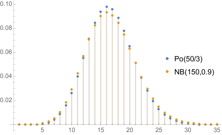
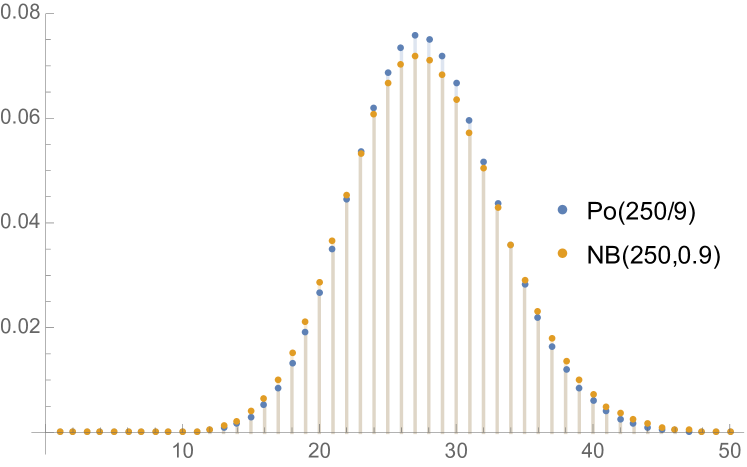
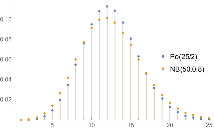
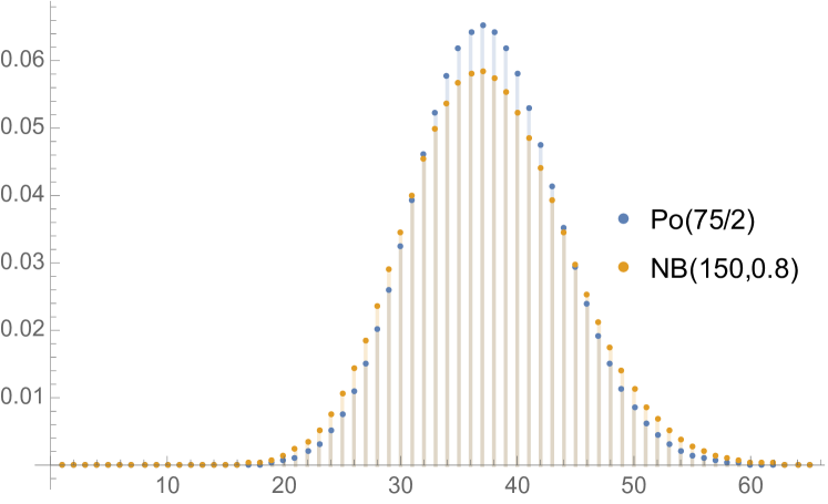
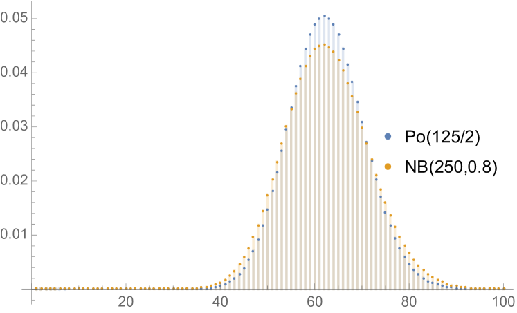
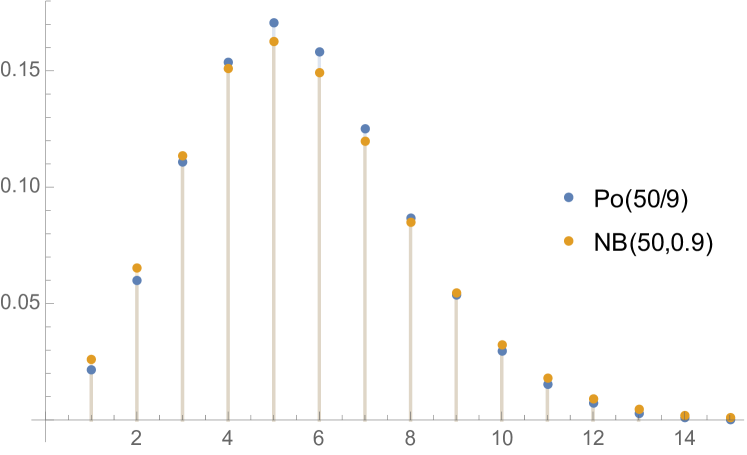
      Note that our bound (from (18)) is better than the bound given in (19). In particular, graphically, the closeness of these two distributions can be seen as follows:

      
      

      Figure 1: $n=10,q=0.1$

      
      

      Figure 2: $n=30,q=0.1$

      
      

      Figure 3: $n=50,q=0.1$

      
      

      Figure 4: $n=10,q=0.2$

      
      

      Figure 5: $n=30,q=0.2$

      
      

      Figure 6: $n=50,q=0.2$

      The above graphs are obtained by using the moment matching conditions. Also, from the numerical table and graphs, observe that the distributions are closer for sufficiently small values of $q$ and large values of $n$, as expected.

   4. From Theorem 1 of Hung and Giang (2016), it is given that, for $A\subset{\mathbb{Z}_{+}}$,

      $$\sup_{A} \left|P(W_{n}\in A)-\sum_{k\in A}\frac{\lambda_{n}^{k}e^{-\lambda_{n}}}{k!}\right|$$

      $$\leq\sum_{i=1}^{n}\min\left\{\lambda_{n}^{-1}(1-e^{-\lambda_{n}})r_{n,i}(1-p_{n,i}),1-p_{n,i}\right\}(1-p_{n,i})p_{n,i}^{-1},$$ (20)

      where $W_{n}=\sum_{i=1}^{n}X_{n,i},\leavevmode\nobreak\ X_{n,i}\sim NB(r_{n,i},p_{n,i})$ with $\lambda_{n}={\mathbb{E}}(W_{n})$. Note that if $\min\left\{\lambda_{n}^{-1}(1-e^{-\lambda_{n}})r_{n,i}(1-p_{n,i}),1-p_{n,i}\right\}=1-p_{n,i}$, for all $i=1,2,\ldots,n$, then

      $$\sup_{A} \left|P(W_{n}\in A)-\sum_{k\in A}\frac{\lambda_{n}^{k}e^{-\lambda_{n}}}{k!}\right|\leq\sum_{i=1}^{n}(1-p_{n,i})^{2}p_{n,i}^{-1},$$ (21)

      which is of order $O(n)$. Clearly, for large values of $n$, Theorem 4.1 is an improvement over (21).

References

• [1] Balakrishnan, N. and Koutras, M. V. (2002). Runs and Scans with Applications. John Wiley, New York.
• [2] Barbour, A. D. (1990). Stein’s method for diffusion approximations. Probab. Theory and Related Fields, 84, 297-322.
• [3] Barbour, A. D. and Chen, L. H. Y. (2014). Stein’s (magic) method. Preprint:arXiv:1411.1179.
• [4] Barbour, A. D., Chen, L. H. Y. and Loh, W. L. (1992a). Compound Poisson approximation for nonnegative random variables via Stein’s method. Ann. Prob., 20, 1843-1866.
• [5] Barbour, A. D., Čekanavičius, V. and Xia, A. (2007). On Stein’s method and Perturbations. ALEA, 3, 31-53.
• [6] Barbour, A. D. and Eagleson, G. K. (1983). Poisson approximation for some statistics based on exchangeable trials. Adv. Appl. Prob., 15, 585-600.
• [7] Barbour, A. D., Holst, L. and Janson, S. (1992b). Poisson approximation. Oxford: Clarendon Press.
• [8] Čekanavičius, V. and Vaitkus, P. (2001). Centered Poisson Approximation via Stein’s Method. Lith. Math. J., 41, 319-329.
• [9] Chen, L. H. Y., Goldstein, L. and Shao, Q.-M. (2011). Normal Approximation by Stein’s Method. Springer, Heidelberg.
• [10] Diaconis, P. and Zabell, S. (1991). Closed form summation for classical distributions. variations on a theme of de Moivre. Statist. Sci., 6, 284–302.
• [11] Goldstein, L. and Reinert, G. (2005). Distributional transformations, orthogonal polynomials and Stein characterizations. J. Theoret. Probab., 18, 237-260.
• [12] Götze, F. (1991). On the rate of convergence in the multivariate CLT. Ann. Prob., 19, 724–739.
• [13] Hirano, K. (1984). Some properties of the distributions of order k. In: A.N. Philippou and A.F. Horadam, eds., Proceedtngs of the First International Conference on Fibonacci Numbers and Their Apphcations (Gutenberg, Athens), pp. 43-53.
• [14] Hung, T. L. and Giang, L. T. (2016). On bounds in Poisson approximation for distributions of independent negative-binomial distributed random variables. Springerplus, 5, 79.
• [15] Huang, W. T. and Tsai, C. S. (1991). On a modified binomial distribution of order k𝑘k. Statist. Probab. Lett.. 11, 125-131.
• [16] Khintchine, A.Ya. (1933). Asymptotische Gesetze der Wahrscheinlichkeitsrechnung. Springer-Verlag, Berlin.
• [17] Kumar, A. N. and Upadhye, N. S. (2017). On perturbations of Stein operator. Comm. Statist. Theory Methods., 46, 9284-9302.
• [18] Le Cam, L. (1960). An approximation theorem for the Poisson binomial distribution. Pacific J. Math., 10, 1181-1197.
• [19] Ley, C. and Swan, Y. (2013a). Stein’s density approach and information inequalities. Electron. Commun. Probab., 18, 1-14.
• [20] Ley, C. and Swan, Y. (2013b). Local Pinsker inequalities via Stein’s discrete density approach. IEEE Trans. Inform. Theory, 59, 5584-5591.
• [21] Ley, C., Reinert, G. and Swan, Y. (2014). Stein’s method for comparison of univariate distributions. Probab. Surv., 14, 1-52.
• [22] Lugannani, R. and Rice, S. O. (1980). Saddle point approximation for the distribution of the sum of independent random variables. Adv. Appl. Probab., 12, 475–490.
• [23] Mattner, L. and Roos, B. (2007). A shorter proof of Kanter’s Bessel function concentration bound. Probab. Theory and Related Fields, 139, 407-421.
• [24] Murakami, H. (2015). Approximations to the distribution of sum of independent non-identically gamma random variables. Math. Sci., 9, 205-213.
• [25] Roos, B. (2003). Kerstan’s method for compound Poisson approximation. Ann. Probab., 31, 1754–1771.
• [26] Reinert, G. (2005). Three general approaches to Stein’s method. An introduction to Stein’s method, Lect. Notes Ser. Inst. Math. Sci. Natl. Univ. Singap., 4, Singapore University Press, Singapore, 183-221.
• [27] Ross, N. (2011). Fundamentals of Stein’s method. Probab. Surv., 8, 210-293.
• [28] Serfozo, R. F. (1986). Compound Poisson approximation for sum of random variables. Ann. Probab., 14, 1391-1398.
• [29] Stein, C. (1986). Approximate computation of expectations. Institute of Mathematical Statistics Lecture Notes-Monograph Series, 7. Institute of Mathematical Statistics, Hayward, CA.
• [30] Stein, C., Diaconis, P., Holmes, S. and Reinert, G. (2004). Use of exchangeable pairs in the analysis of simulations. In Stein’s Method: Expository Lectures and Applications (P. Diaconis and S. Holmes, eds.). IMS Lecture Notes Monogr. Ser 46 1–26. Beachwood, Ohio, USA: Institute of Mathematical Statistics.
• [31] Upadhye, N. S., Čekanavičius,V. and Vellaisamy, P. (2014). On Stein operators for discrete approximations. Bernoulli, 23, 2828-2859.
• [32] Vellaisamy, P., Upadhye, N. S. and Čekanavičius, V. (2013). On Negative Binomial Approximation. Theory Probab. Appl., 57, 97-109.
• [33] Vellaisamy, P. and Upadhye, N. S. (2009). Compound negative binomial approximations for sums of random variables. Probab. Math. Statist., 31, 205-226.
• [34] Yakshyavichus, Sh. (1998). On a method of expansion of the probabilities of lattice random variables. Theory Probab. Appl., 42, 271-282.