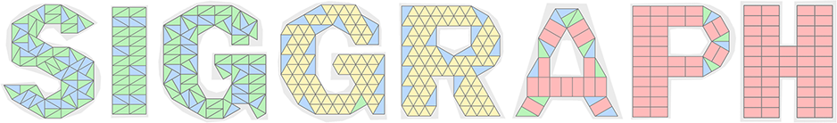
Figure 1. Our self-supervised neural network, TilinGNN, produces tiling results in time roughly linear to the number of candidate tile locations, significantly outperforming traditional combinatorial search methods. The average runtime of our network for tiling a character is only 25.71s. The character shapes to be tiled are shown in grey and different types of tiles are displayed using different colors (note that mirror reflections count as different tile types).

TilinGNN: Learning to Tile with Self-Supervised Graph Neural Network

Abstract.

We introduce the first neural optimization framework to solve a classical instance of the tiling problem. Namely, we seek a non-periodic tiling of an arbitrary 2D shape using one or more types of tiles—the tiles maximally fill the shape’s interior without overlaps or holes. To start, we reformulate tiling as a graph problem by modeling candidate tile locations in the target shape as graph nodes and connectivity between tile locations as edges. Further, we build a graph convolutional neural network, coined TilinGNN, to progressively propagate and aggregate features over graph edges and predict tile placements. TilinGNN is trained by maximizing the tiling coverage on target shapes, while avoiding overlaps and holes between the tiles. Importantly, our network is self-supervised, as we articulate these criteria as loss terms defined on the network outputs, without the need of ground-truth tiling solutions. After training, the runtime of TilinGNN is roughly linear to the number of candidate tile locations, significantly outperforming traditional combinatorial search. We conducted various experiments on a variety of shapes to showcase the speed and versatility of TilinGNN. We also present comparisons to alternative methods and manual solutions, robustness analysis, and ablation studies to demonstrate the quality of our approach. Code is available at https://github.com/xuhaocuhk/TilinGNN/

1. Introduction

Many geometry processing tasks in computer graphics require solving discrete and combinatorial optimization problems, e.g., decomposition, packing, set cover, and assignment. Conventional approaches resort to approximation algorithms with guaranteed bounds or heuristic schemes exhibiting favorable average performance. With the rapid adoption of machine learning techniques in all facets of visual computing, an intriguing question is whether difficult combinatorial problems involving geometric primitives can be effectively and efficiently solved using a machine learning approach.

In this paper, we explore a learning-based approach to solve a combinatorial geometric optimization problem, tiling, which has drawn interests from the computer graphics community in different contexts (Kaplan, 2009), e.g., sampling (Kopf et al., 2006; Ostromoukhov, 2007), texture generation (Cohen et al., 2003), architectural construction (Fu et al., 2010; Eigensatz et al., 2010; Singh and Schaefer, 2010), and puzzle design (Duncan et al., 2017). In general, tiling refers to the partition of a domain into regions, the tiles, of one or more types. So far, most works on tiling have stayed in the 2D domain; see Figure 2 for some typical examples and applications.

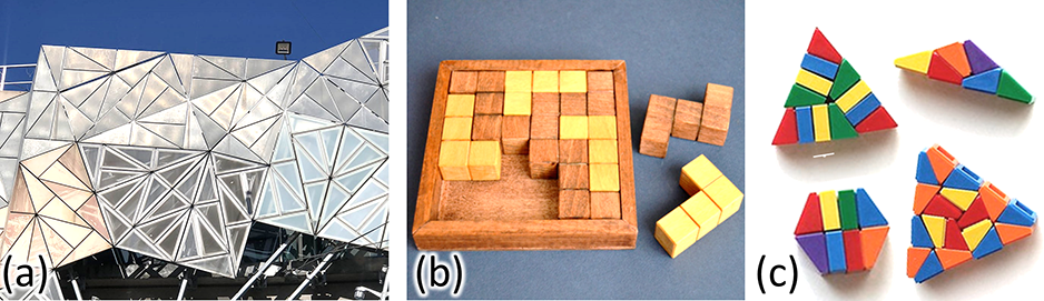
Figure 2. Applications of tilings: (a) Federation Square in Melbourne; (b) a puzzle called jags and hooks designed by Erhan Cubukcuoglu; and (c) cheese slope mosaic using LEGO bricks from Katie Walker’s Flickr page.

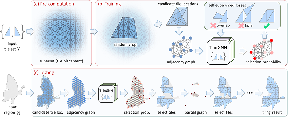
Figure 3. Overview of our “learn-to-tile” approach: (a) we precompute a “superset” of candidate tile locations for each given tile set; (b) we train our graph neural network TilinGNN to learn to tile for the given tile set by generating random 2D shapes to locate full tile placements inside both the superset and random shape and then by training TilinGNN to learn to predict locations to place tiles in a self-supervised manner; and (c) given a region to tile, we first locate candidate tile locations within the region, then make use of the trained network model to progressively select tile locations and generate the tiling result.

As a first attempt, we focus on non-periodic tiling of an arbitrary 2D shape using one or more types of tiles. Specifically, we seek a tiling that maximally fills the shape’s interior without overlaps, holes, or tiles exceeding the shape boundary. Even such an elementary version of the tiling problem is hard—it is known that whether a finite 2D region can be tiled with a given set of tiles is NP-complete, even when the tile set has only one type such as the tromino (Moore and Robson, 2001). Existing open-source libraries such as COIN-OR/BC (2018) (for branch & cut mixed integer programming) and commercial combinatorial optimization tools such as Gurobi (2020) (specialized integer programming solver) are alternatives to solving our tiling problem. They are, however, very time-consuming, e.g., we found empirically that Gurobi took over five minutes to produce a tiling solution for one character shown in Figure 1. Our goal is to resort to a data-driven approach, which can produce very good, while not necessarily optimal, solutions at much greater efficiency.

In general, the solution space for tiling is immense, spanning both a discrete search for tile type selection and arrangement, as well as a continuous search for tile orientation and positioning. Also, we must respect hard constraints related to input boundary, holes, and tile overlaps. A traditional approach to solving the problem would search over the space of tile selection and placement, progressively laying out tile instances to fill the tiling region, possibly with trial-and-error and backtracking in the solution search. However, the ensuing computation would be prohibitively expensive.

By taking a learning-based approach, we train a deep neural network, whose parameters encode knowledge or patterns of the tiling solutions. At test time, the learned patterns would guide the tile placement, instead of relying on expensive on-line search. Specifically, we model our tiling problem as an instance of graph learning. In our graphs, nodes represent candidate tile locations in the solution space and edges encode tile overlap relations and regular tile connections. Such a representation allows us to adopt a graph neural network, which is coined TilinGNN, to process features on graph nodes. These features are aggregated along graph edges, via graph convolution, to predict tile locations for inclusion in the solution.

Structure-wise, TilinGNN has a two-branch network architecture with a series of neighbor aggregation modules and overlap aggregation modules to learn features related to tile connection and overlap. In such a way, we train TilinGNN to learn to maximize the tiling solution coverage, while avoiding tile overlaps and holes. Importantly, we formulate these tiling criteria as loss terms, which are functions of the network outputs. Hence, our network can be trained in a self-supervised manner, without the need for any human-provided tiling solutions as ground truth during the training.

The runtime of using a trained TilinGNN model to tile a shape is roughly linear to the number of candidate tile locations. Typically, we can generate a tiling solution in less than a minute, which is hard to achieve using tiling approaches based on traditional combinatorial search. To verify this, we perform experiments to compare our method with COIN-OR/BC (2018) and Gurobi (2020) for tiling different shapes of varying sizes. The results confirm the superior speed and tiling quality of our method. Besides, we showcase a variety of tilings produced by our method using assorted tile sets with single or multiple tile types (see Figure 1), present an interactive design tool, compare our results with manual solutions, and present various evaluations on the network architecture and loss.

To the best of our knowledge, TilinGNN represents the first attempt at generating non-periodic tilings using a deep neural network. Since this form of tiling is only one particular instance of the more general problem setting of “learning to select” over a graph structure, we believe that our approach can bring insights and open up new directions for solving other similar combinatorial problems in computer graphics research, e.g., the design of hybrid meshes  (Peng et al., 2018) and various computational assembly problems (Luo et al., 2012; Deuss et al., 2014; Xu et al., 2019c).

2. Related work

Generally speaking, machine learning enables a computer system to perform tasks without pre-defining model features or providing explicit instructions. Instead, the features and computational parameters behind the actions are automatically learned from data rather than being fixed or handcrafted. Most deployments of machine learning techniques to computer graphics can be found in image and video processing, e.g., (Bau et al., 2019; Sun et al., 2019; Jamriška et al., 2019), where conventional convolutional processing over regular grid data are typically applied. Recently, some success has been achieved in geometric deep learning over irregular data such as shapes (Li et al., 2017; Mo et al., 2019) and scene structures (Wang et al., 2019; Li et al., 2019; Gao et al., 2019), which are represented as attributed trees or graphs. What is common about these methods is that they are supervised, where the networks were trained to learn structural consistencies in a shape/scene collection arising from shared semantic or functional attributes.

In contrast, our goal is to develop a self-supervised tiling solution that works on arbitrary input shapes without assuming any shared commonality among them. In this section, we discuss relevant works to the tiling problem, including image and pattern generation, shape decomposition, and 3D shape assembly. A coverage on neural combinatorial optimization models is also provided.

Tiling for image and pattern generation.

Artists, graphics designers, and mathematicians have been interested in the problem of tilings and their properties for centuries. Theories and in-depth analysis of most instances of the tiling problem can be found in (Grünbaum and Shephard, 1986). Existing works focus mostly on filling the 2D plane using a small set of fixed shapes as the tiles, for example, the periodic and aperiodic tilings, and polyomino tilings. In computer graphic research, various tools have been developed to help produce different kinds of intriguing tiling patterns. For example, the problem of Escherization (Kaplan and Salesin, 2000), creation of decorative mosaics using colored tiles (Hausner, 2001; Smith et al., 2005), texture generation with Wang tiles (Stam, 1997; Cohen et al., 2003), object distribution on the plane (Hiller et al., 2003), the construction of traditional Islamic star patterns (Kaplan and Salesin, 2004), and the design of artistic packing layouts (Reinert et al., 2013). These works focus either on the mathematics to support the tiling constructions, or on methods with heuristics such as Voronoi Diagrams to divide the plane and fill it with tiles.

Decomposition.

A line of works that bears some resemblance to tiling follows the principle of design by composition. However, the ensuing decomposition problem is characteristically different from tiling, since the compositional elements are not of fixed shapes; they typically share some common geometric or appearance properties, but are otherwise of different shapes, even deformable. Also, there is often a desire to minimize the decomposition size. Literatures on decomposition are vast. Some exemplary works include image mosaics (Kim and Pellacini, 2002; Xu et al., 2019a), shape collages (Huang et al., 2011; Kwan et al., 2016), convex decomposition (Lien and Amato, 2004), ornamental packing (Saputra et al., 2017), fabricable tile decors (Chen et al., 2017), approximate dissection (Duncan et al., 2017), and reversible linked dissection (Li et al., 2018b).

Assemblies of fixed blocks.

Assembling a shape using a small set of building blocks may also be viewed as a form of tiling. Eigensatz et al. (2010), Fu et al. (2010), and Singh and Schaefer (2010) independently develop methods for the problem of constructing a small set of shapes (or panels) that together can tile a given 3D surface. Peng et al (2014) tackle the problem of tiling a domain with a set of deformable templates. Luo et al. (2015) account for the shape, colors, and physical stability when their method searches for LEGO brick constructions. Skouras et al. (2015) develop a design tool to build structures from interlocking quadrilateral elements. Chen et al. (2018) compute an internal core built by universal blocks to support a 3D-printed shell, Xu et al. (2019c) search for 3D LEGO Technic brick constructions, given the user-input sketches, while Peng (2019) design 2D checkerboard patterns with black rectangles derived from quad meshes. In general, computational assembly problems, including ours, are combinatorial by nature, so they are typically solved by integer programming (IP) or heuristic search. Being general tools for combinatorial problems, IP solvers could be rather time-consuming for large problems. On the other hand, specifically-designed heuristic search could perform fast, but it may not be general for solving problems of different forms. In our work, we trade-off the advantages of the two approaches, and leverage a graph neural network to learn the solution patterns as heuristics, so that we can make fast predictions using the trained model.

Graph neural networks (GNNs).

A natural extension from regular grid processing to deal with irregularly structured data is to utilize graph representations. There has been much recent development on deep learning using graph neural networks (GNNs) (Wu et al., 2019), in particular, graph convolutional networks (GCNs), which our method adopts. GCNs build stacked convolutional layers over graph structures to enable feature aggregation based on neighborhood information. Some recent works from computer graphics apply GCNs in different contexts. In MeshCNN, Hanocka et al. (2019) perform graph convolution and pooling over mesh edges. In PlanIT, Wang et al. (2019) develop a GCN-based generative model for indoor scenes, where the network operates on scene graphs that encode object-to-object relations. In StructureNet, Mo et al. (2019) encode 3D shapes using $n$-ary graphs and consider both part geometry and inter-part relations in the network training. In our work, GCNs are applied in a novel way for tiling, where the graph encodes the tile overlap and connection relations, and the network is trained to predict probabilities for tile selection and placement.

Neural combinatorial optimization.

Recent works on neurally guided optimization explore data-driven and learning-based schemes for solving discrete and combinatorial problems. A typical and notable example is Alpha Go (Silver et al., 2017), which trains a machine to predict the best next move in Go play using Monte Carlo tree search. Many works attempt to use machine learning to efficiently solve classical NP-hard problems such as traveling salesman (Vinyals et al., 2015; Bello et al., 2016; Dai et al., 2017), boolean satisfiability (Yolcu and Póczos, 2019), maximum independent set (Li et al., 2018a; Abe et al., 2019), graph coloring (Lemos et al., 2019), and maximum cut (Dai et al., 2017; Yolcu and Póczos, 2019). The particular learning-based mechanisms include recurrent neural networks, attention models, deep reinforcement learning, as well as GCNs.

The common insight of these works is to train a neural network to predict selection probabilities over discrete options, and use a simple selection strategy (e.g., greedy) to incrementally construct a solution, as guided by the probabilities. Our work inherited the same spirit, where we model the tile placements as discrete options, but differs in the way of the learning process. To train a network, we neither have a data set of tiling solutions to supervise the training, nor train in a reinforcement learning framework via trials and errors. Instead, we formulate losses to evaluate the quality of the network output, training the network in a self-supervised manner.

3. Overview

Problem definition.

Given a set $\mathcal{T}$ of a few simple 2D shapes representing the input tile types, and a connected region $\mathcal{R}$ in 2D, we aim to arrange instances of tiles from $\mathcal{T}$ over $\mathcal{R}$ without overlap or hole between the tile instances, such that the resulting tiling can maximally cover the interior of $\mathcal{R}$ without exceeding its boundary. Figure 4 shows an illustration of the problem.

Note that we can rotate and translate the tiles, but not flip or scale them, when arranging the tile instances. Since the shape of $\mathcal{R}$ is arbitrary and the tile set is limited, completely filling the entire $\mathcal{R}$ may not be always possible, as demonstrated by the example shown in Figure 4(c). Last but not least, the region $\mathcal{R}$ itself may contain holes, as shown by characters “A” and “R” in Figure 1.

Overall, the problem setting is quite general, covering an infinite number of problem instances. When considering different tile sets and tiling regions as inputs, the difficulty of the problem varies. For example, tiling a general 2D region using trominoes has been proved to be NP-complete (Moore and Robson, 2001), while tiling a square region using smaller squares is relatively easy.

Challenges.

First, the search space is immense, as we must handle three closely-coupled sub-problems: (i) which tile to pick; (ii) how to position and orientate each tile; and (iii) how many instances of each tile type to use in the tiling. The decision variables of problems (i) & (iii) are discrete, while those of problem (ii) are continuous.

Second, the avoidances of overlaps, holes, and tiles surpassing the input shape boundary are all hard constraints. In general, we need to actively evaluate the tile placements against these constraints and discard those that violate the constraints; this can be exceedingly time-consuming given the immense search space.

Finally, tile placements require both local and global considerations. Locally, the placement of a tile is closely related to the placements of the neighboring tiles, so that we can avoid the tile overlap and minimize the gaps between tiles to maximally cover $\mathcal{R}$. Globally, a change in a local tile placement can subsequently affect its neighbors and even the entire tiling, since the hard constraints can propagate over the neighbors successively over the tiling.

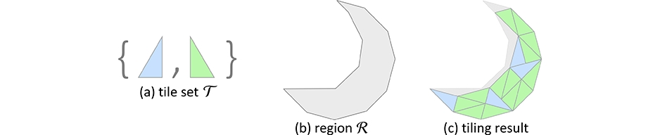
Figure 4. The tiling problem. Given a tile set $\mathcal{T}$ (a) and a 2D region $\mathcal{R}$ to be filled (b), we aim to produce a tiling (c) that maximally covers the interior of the given region without overlap or hole between the tile instances.

Our approach.

In this work, we explore a new approach by designing and training a graph neural network with self-supervised losses to learn to predict tile placement locations. Then, at test time, we can make use of the network to generate tiling efficiently. Altogether, our approach has three phases, as illustrated in Figure 3:

• Given an input tile set $\mathcal{T}$, we first pre-compute a superset of tile configurations that enumerates all candidate tile placement locations for $\mathcal{T}$; see Figure 3(a) and Section 4.

• Our next goal is to train a GNN, coined TilinGNN, to learn to predict tile placement locations for the given tile set; see Figure 3(b). To do so, we generate a random 2D shape to crop a tiling configuration so as to locate candidate tile locations inside the shape. Then, we create a graph structure to describe the adjacency between candidate tile locations in the shape and train TilinGNN to predict tile placement locations by formulating self-supervised losses to avoid overlaps and holes in the tiling. We repeat this process using many different random shapes, as a means for data augmentation, to facilitate the training of TilinGNN; see Section 5.

• To fill a test region, we first locate candidate tile locations within the region, then fill the region by using the TilinGNN trained on the target tile set to progressively predict tile placements; see Figure 3(c) and Section 5.4 for details.

4. Modeling the Tiling Problem

To adopt a neural network to perform tiling is non-trivial. First, the input data, i.e., both the tiling region $\mathcal{R}$ and the tiles in $\mathcal{T}$, have irregular shapes, so we cannot directly process them by conventional convolutional neural networks. Second, the tiling problem can have many different problem instances, when using different tile sets to tile different kinds of regions. The neural network architecture should be general to handle them in a unified fashion. Lastly, the number of tiles in the input tile set is not fixed, whereas the number of tiles in the output tiling is unknown. The approach should be able to allow such flexibility for both the inputs and outputs.

Hence, we approach the problem by first modeling the tile set and enumerating the candidate tile locations (Section 4.1). Then, we model the problem of tiling generation as a graph problem and present necessary constraints and objectives (Section 4.2). These are preparation works to later enable processing by TilinGNN.

4.1. Modeling the Tile Set and Tile Placements

First, we state two fundamental requirements on the tile set $\mathcal{T}$:

• $\mathcal{T}$ should seamlessly tile the plane, such that the tile instances may fill target region $\mathcal{R}$ without holes and tile overlaps; and

• the tile set and tile connection rules together should induce a finite number of candidate tile locations inside a finite region. Indeed, since TilinGNN is a selection network, it has to operate on a finite number of candidate choices. The candidate tile locations, or the superset, should then form a periodic grid, e.g., see Figure 3(a). However, the generated tilings, formed by selected candidate tiles, can be far from periodic.

Figure 5 shows some of the tile sets supported by TilinGNN.

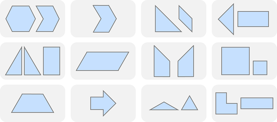
Figure 5. Exemplary tile sets. Some of them have specific names, e.g., the rightmost two at the bottom are the labyrinth tiles and tromino tiles.

Figure 6. For the example tile set given in (a), there are twelve possible ways to place a neighbor (b) around the right-angled tile marked in yellow.

Tile neighbors.

In general, the neighbor of a tile can be placed at any location next to the tile, as long as they contact by an edge or a point. In this work, we consider only neighbors that contact by a common edge segment and do not allow the neighbor to continuously slide over the contacting edge, since this induces an infinite number of candidate tile placements (see top-left case in inset figure below). Besides sharing a full edge (see top-middle case in inset figure), if a

side length of a tile is a multiple of some shorter side lengths in the whole tile set, the tiles can then connect with “quantized” lengths along the shared edge (see bottom three cases in inset figure). See also Figure 6, for more examples of the neighbor tile placement locations.

Candidate tile placements.

Based on the above tile connection rule, we can determine a finite set of candidate tile placement locations over a given region. We denote such a set as $\mathcal{P}$. To find $\mathcal{P}$ for a given tile set, one way is to pick one of the tile(s) in the tile set as a seed, locate all possible neighbors around the seed (see Figures 7 (a)-(c) for examples), then repeat the process recursively with the neighbors, until we fill the target region (see Figure 7(d)). Besides, for the tromino tile set shown at the bottom right corner of Figure 5, we can simply sweep each tile type over a regular 2D grid for each unique orientation of the tile type to find $\mathcal{P}$ of the tile set.

Clearly, the size of $\mathcal{P}$ grows with the region size and the complexity of the tile set, we thus limit the size of $\mathcal{P}$ by the available GPU memory. Typically, our current implementation of TilinGNN on a single GPU can work with $\sim$5k (candidate) tile locations.

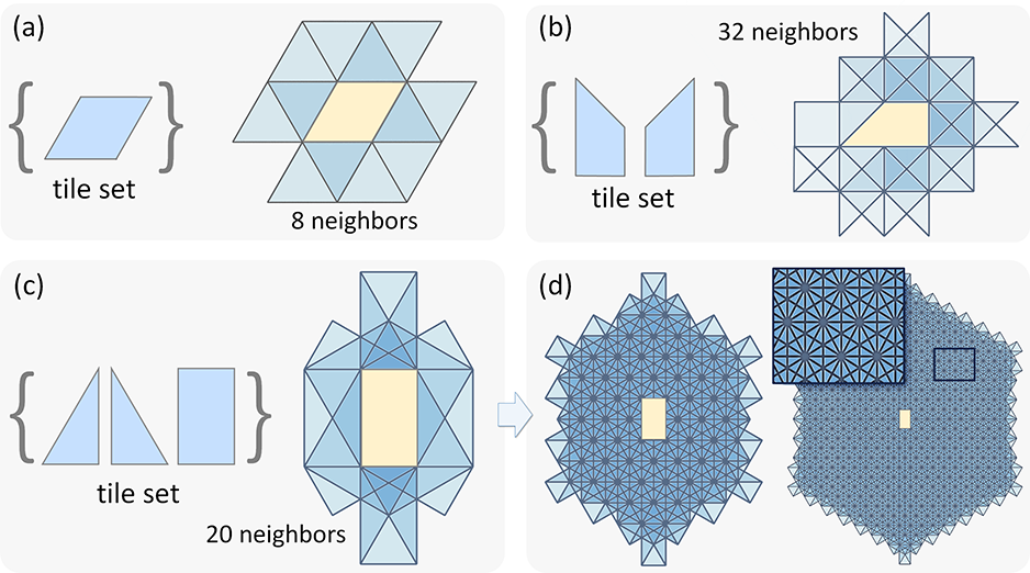
Figure 7. (a)-(c) Given a tile set, we pick one of its tiles as the seed (yellow) and locate all surrounding neighbors, which are rendered in transparent altogether. (d) If we repeat the process recursively with the neighbors, we can find the candidate tile placement locations over larger regions, e.g., there are 742 (left) and 5301 (right) tile locations in these two results.

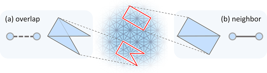
Figure 8. The two types of edges in the adjacency graph: (a) an overlap edge (dashed line) between nodes, of which the tile locations overlap; and (b) a neighbor edge (solid line) between nodes, of which the tile locations contact.

4.2. Modeling Tiling as a Graph Problem

By means of modeling the candidate tile placement locations, a tiling problem can be cast as a graph problem for TilinGNN to work on. That is, given a region $\mathcal{R}$ to tile, we can first locate a set of candidate tile placement locations in the region. We can then create an adjacency graph (denoted by $\mathcal{G}$) to describe the connectivity between candidate tile locations by regarding each candidate tile location as a graph node, and construct edges for two cases:

• If two candidate tile locations overlap each other, we construct an overlap edge to connect their respective nodes in $\mathcal{G}$; and

• If two candidate tile locations contact each other by an edge segment without any overlap, we construct a neighbor edge to connect their respective nodes in $\mathcal{G}$.

Figures 8 (a) & (b) illustrate these two types of edges. We use dashed lines and solid lines to denote overlap and neighbor edges, respectively; see also the adjacency graph example in Figure 3(b).

Therefore, adjacency graph $\mathcal{G}$ is an undirected graph that can be written as $\mathcal{G}=\{\mathcal{V},\mathcal{E}_{\text{ovl}},\mathcal{E}_{\text{nbr}}\}$ with node set $\mathcal{V}$, overlap edge set $\mathcal{E}_{\text{ovl}}$, and neighbor edge set $\mathcal{E}_{\text{nbr}}$. In this way, we can re-formulate our tiling problem as the problem of

Finding a (maximum) subset of nodes in $\mathcal{G}$, such that all adjacent nodes are connected by edges in $\mathcal{E}_{\text{nbr}}$ and no two nodes are connected by any edge in $\mathcal{E}_{\text{ovl}}$.

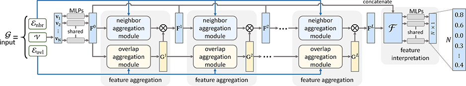
Figure 9. The overall architecture of TilinGNN is a two-branch graph convolutional neural network. The network progressively propagates and aggregates node features ($\mathbf{F}^{l}$ and $\mathbf{G}^{l}$) over the neighbor and overlap edges in an adjacency graph, using the neighbor aggregation and overlap aggregation modules (see Figure 10) to predict node selection probabilities for candidate tile placements in tiling generation. $N$ is the total number of nodes in the graph; both $\mathbf{F}^{l}$ and $\mathbf{G}^{l}$ are node features of dimensions $N\times C$; $C$ is the number of feature channels; $L$ is the number of layers in TilinGNN; and $\otimes$ is the element-wise product.

Here, we aim to find a tiling that maximally covers tiling region $\mathcal{R}$ without holes and tile overlaps. Such a problem can be further cast as an optimization, in which we select a subset of nodes in $\mathcal{G}$, such that (i) the total area of the tiles associated with the selected nodes is maximized; (ii) we aim to avoid holes between tiles, by maximizing

the total length of contacting edges between all adjacent nodes (see the right inset figure for illustrations); and (iii) we have a hard constraint that no two nodes are connected by edges in $\mathcal{E}_{\text{ovl}}$.

5. TilinGNN for Tiling Generation

In this section, we first present the inputs we feed to TilinGNN (Section 5.1), the architecture of TilinGNN (Section 5.2), and the loss function we formulated for self-supervised training (Section 5.3). Then, we present the procedure to employ a trained TilinGNN model to tile a given shape or region (Section 5.4).

5.1. Neural network inputs

In each iteration to train TilinGNN, we start by using a random 2D shape to crop and locate a subset of candidate tile locations in the “superset” of the target tile set $\mathcal{T}$; see again Figure 3(b). Note again that TilinGNN is trained per tile set. Then, we construct an adjacency graph $\mathcal{G}=\{\mathcal{V},\mathcal{E}_{\text{ovl}},\mathcal{E}_{\text{nbr}}\}$ to describe the connection and overlap relations between the cropped candidate tile locations, following the procedure presented in Section 4.2. Besides $\mathcal{G}$, we prepare the following two sets of inputs to train TilinGNN:

• Per-node vectors $\{\mathbf{v}_{i}\}$. To start, we denote $N$ as the number of nodes in $\mathcal{V}$ and $N_{t}$ as the number of tile types in $\mathcal{T}$. Also, we denote $A_{i}$ as the area of the tile ($i$-th candidate tile location) associated with the $i$-th node in $\mathcal{V}$ after normalized by the maximum tile area, i.e., $\max(A_{i})$. Then, we prepare an $(N_{t}$$+$$1)$-dimensional vector $\mathbf{v}_{i}$ per node in $\mathcal{V}$, where $i\in\{1,...,N\}$, the first element of $\mathbf{v}_{i}$ is $A_{i}\in[0,1]$ and the remaining $N_{t}$ elements is a one-hot vector (a single ‘1’ with all the other ’0’s) representing which of the $N_{t}$ tiles (i.e., tile type) in $\mathcal{T}$ associated with the $i$-th candidate tile location.

• Per-neighbor-edge vectors $\{\mathbf{e}_{j}\}$. We denote $N_{e}$ as the number of neighbor edges in $\mathcal{E}_{\text{nbr}}$ and $N_{p}$ as the number of all different relative poses between connectable tiles in $\mathcal{T}$, e.g., for the tile sets shown in Figures 7 (a) & (b), $N_{p}$ are $8$ and $32$, respectively. Also, we denote $L_{\max}$ as the maximum perimeter among the perimeters of all tile types in $\mathcal{T}$, and compute the length of the shared edge segment for each of the $N_{p}$ relative poses. Then, we prepare an $(N_{p}$$+$$1)$-dimensional vector $\mathbf{e}_{j}$ per neighbor edge in $\mathcal{E}_{\text{nbr}}$, where $j\in\{1,...,N_{e}\}$, the first element of $\mathbf{e}_{j}$ is the length of the shared edge segment associated with the $j$-th neighbor-edge connection in $\mathcal{E}_{\text{nbr}}$ after normalized by $L_{\max}$, and the remaining $N_{p}$ elements is a one-hot vector representing which of the $N_{p}$ relative poses that the $j$-th neighbor edge associates with.

Note that we do not extract extra information for the overlap edges in $\mathcal{G}$, since overlap is a hard constraint and we must avoid all kinds of overlap connections. Also, while there are many other geometric and topological information that we may include in $\{\mathbf{v}_{i}\}$ and $\{\mathbf{e}_{j}\}$, e.g., the coordinates of the tile location and orientation angle, we do not find them helpful in training TilinGNN.

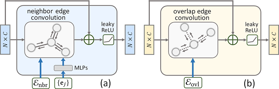
Figure 10. Illustration of the neighbor aggregation module (a) and the overlap aggregation module (b) inside TilinGNN shown in Figure 9.

Figure 11. Visualizing the network outputs when using TilinGNNs trained for different number of epochs to test on the Tortoise shape. Note that we render the candidate tile placements from low (yellow) to high (green) network-output probabilities, so those with high probabilities are less occluded. From the results, we can see that TilinGNN can gradually learn over the training process to give higher probabilities to select non-overlapping and connecting tiles.

5.2. Network Architecture

Figure 9 shows the overall architecture of TilinGNN, whereas Figure 10 shows the detailed structure of two major modules inside TilinGNN, i.e., the neighbor aggregation and overlap aggregation modules. Overall, TilinGNN is a two-branch graph convolutional neural network that progressively propagates and aggregates node features over the neighbor edges and overlap edges. Here, we denote $\mathbf{F}^{l}$ and $\mathbf{G}^{l}$ as the node features for the two modules, where $l$ is a nonnegative integer that denotes layer. The inputs to TilinGNN include an adjacency graph $\mathcal{G}$ and the associated per-node and per-edge information $\{\mathbf{v}_{i}\}$ and $\{\mathbf{e}_{j}\}$, whereas its output is a vector of $N$ values, indicating the probability of selecting each node in $\mathcal{G}$, i.e., a candidate tile location, for the tiling generation.

From left to right in the network architecture diagram shown in Figure 9, TilinGNN first uses a set of shared multi-layer perceptrons (MLPs) to process $\{\mathbf{v}_{i}\}$ and generate node feature $\mathbf{F}^{0}$ (dimension: $N\times C$), which is a set of $N$ per-node feature vectors, each of $C$ channels. Then, we pass $\mathbf{F}^{0}$ independently into a neighbor aggregation module and an overlap aggregation module, which form the first feature aggregation layer. The output of the neighbor aggregation module is then aggregated (multiplied) with the output of the overlap aggregation module, which is $\mathbf{G}^{0}$ (dimension: $N\times C$), to produce node feature $\mathbf{F}^{1}$. In this way, we can propagate each node feature vector in $\mathbf{F}^{0}$ through the node’s associated neighbor edge(s) and overlap edge(s) in the adjacency graph for one step.

To enable TilinGNN to learn effective node features, we should further propagate the node features for more steps over the graph, which is essentially the spatial domain for tiling. Hence, we further feed $\mathbf{F}^{1}$ into the second feature aggregation layer, etc., and subsequently generate $\mathbf{F}^{2}$ up to $\mathbf{F}^{L}$, where $L$ is the number of feature aggregation layers in TilinGNN. In the end, we produce the overall node feature $\mathcal{F}$ (dimension: $N\times C\times(L+1)$) by concatenating all the node features $\{\mathbf{F}^{0},\mathbf{F}^{1},...,\mathbf{F}^{L}\}$. We then feed $\mathcal{F}$ into a set of shared MLPs with sigmoid activation to map each node feature vector in $\mathcal{F}$ to predict a probability value. Note also that we set $L=20$ and $C=64$; see the implementation details in Section 6.

Neighbor aggregation module

This module focuses on aggregating node features over neighbor edges $\mathcal{E}_{\text{nbr}}$; see Figure 10(a). We denote $\mathbf{F}^{l}=\{\mathbf{f}^{l}_{1},\mathbf{f}^{l}_{2},...,\mathbf{f}^{l}_{N}\}$ as the node features in the $l$-th layer. From $\mathcal{E}_{\text{nbr}}$, $\mathbf{F}^{l}$, and $\{\mathbf{e}_{j}\}$, the module first uses a set of shared MLPs (for $l$-layer) to process $\{\mathbf{e}_{j}\}$ and generate $\Phi^{l}(\mathbf{e}_{j})$ per edge in $\mathcal{E}_{\text{nbr}}$. The dimension of $\Phi^{l}(\mathbf{e}_{j})$ is $C\times C$. Then, we employ an edge-conditioned convolution layer (Simonovsky and Komodakis, 2017) to aggregate features from the neighboring nodes (along neighbor edges) conditioned on the associated edge features for each node, with leaky ReLU (denoted as LReLU) as the activation output function:

(1) $$\mathbf{f}^{l+1}_{i}=\mathrm{LReLU}\big{(}\mathbf{f}^{l}_{i}\cdot W^{l}+\sum_{\{k,j\}\in N_{\text{nbr}}(i)}\mathbf{f}^{l}_{k}\cdot\Phi^{l}(\mathbf{e}_{j})\big{)}\ ,$$

where $W^{l}$ is learnable weight (dimension: $C\times C$) and $N_{\text{nbr}}(i)$ is the set of indices of nodes ($k$) and edges ($j$) connected with the $i$-th node in $\mathcal{V}$ via neighbor edges. Also, we add residual connections in the module (see again Figure 10(a)) to avoid the problem of vanishing gradient (He et al., 2016), since the network is deep.

Overlap aggregation module

Similar to the neighbor aggregation module, the overlap aggregation module also takes the node feature from the previous layer as input. Typically, its input node feature can be $\mathbf{F}^{0}$ (for 1st layer) or $\mathbf{G}^{l}$ (for 2nd to $L$-th layers); see Figure 9. For simplicity, we denote it as $\mathbf{G}^{l}=\{\mathbf{g}^{l}_{1},\mathbf{g}^{l}_{2},...,\mathbf{g}^{l}_{N}\}$. Then, we employ the convolution layer proposed by (Xu et al., 2019b) to perform convolutions on the overlap edges for each node:

(2) $$\mathbf{g}^{l+1}_{i}=\mathrm{LReLU}\big{(}\Theta^{l}\big{(}(1+\epsilon{\color[rgb]{0,0,0}{}^{l}})\mathbf{g}^{l}_{i}+\sum_{k\in N_{\text{ovl}}(i)}\mathbf{g}^{l}_{k}\big{)}\big{)},$$

where $\epsilon{\color[rgb]{0,0,0}{}^{l}}$ is a learnable value (initialized as zero and modified adaptively by the network optimizer); $N_{\text{ovl}}(i)$ is the set of indices of nodes ($k$) connected with the $i$-th node in $\mathcal{V}$ via overlap edges; and $\Theta^{l}(\cdot)$ is a differentiable function implemented by a set of shared MLPs using also leaky ReLU as the activation function. Note that we use a different mechanism to aggregate overlap-related node features, since (Xu et al., 2019b) has been shown to be effective for scenarios, in which the graph has no edge labels.

Discussion

TilinGNN can also be viewed as a binary classification network on nodes in the adjacency graph, such that nodes predicted with high (or low) probability are likely (or unlikely) belonging to the final tiling. However, unlike general classification problems, we have a large amount and different types of edge connections in our graph, and the selected high-probability nodes should not locate next to one another, due to the overlap constraint. Hence, we cannot directly employ existing classification networks to our problem.

5.3. Loss Function

We denote $x_{i}\in[0,1]$ as the network-output probability of selecting the $i$-th node (candidate tile location) in $\mathcal{G}$. Similar to (Leimkühler et al., 2019), we formulate loss terms on $x_{i}$ to train TilinGNN in a self-supervised manner, where $w_{\text{a}}$, $w_{\text{o}}$, and $w_{\text{e}}$ below are weights:

• To maximize the tiling coverage of the target region, we make use of the normalized tile area $A_{i}$ (see Section 5.1) to define

  $$L_{\text{a}}\ =\ 1-w_{\text{a}}\log_{e}(\frac{\sum_{i}A_{i}x_{i}}{\sum_{i}A_{i}})\ .$$

• To minimize the tile overlaps, we define

  $$L_{\text{o}}\ =\ 1-w_{\text{o}}\cdot\frac{1}{\left|\mathcal{E}_{\text{ovl}}\right|}\sum_{\{i,k\}\in\mathcal{E_{\text{ovl}}}}\log_{e}(1-x_{i}x_{k})\ .$$

• To avoid holes among the selected tile locations, we maximize the total length of the contacting edge segments between the nodes connected by neighbor edges, and define

  $$L_{\text{e}}\ =\ 1-w_{\text{e}}\cdot\frac{1}{\left|\mathcal{E}_{\text{nbr}}\right|}\sum_{\{i,k\}\in\mathcal{E_{\text{nbr}}}}\log_{e}(\frac{x_{i}x_{k}L_{i,k}}{L_{\max}})\ ,$$

  where $L_{i,k}$ is the length of the contacting edge segment between the $i$-th and $k$-th nodes, and $L_{\max}$ is the maximum tile perimeter, as defined earlier in Section 5.1.

Then, we formulate the overall loss as a product of $L_{\text{a}}$, $L_{\text{o}}$, and $L_{\text{e}}$, and aim to minimize this overall loss in the network training. In our initial attempt, we use a weighted sum to combine the three terms, but the network training does not converge and yields poor results. Our log-based design is inspired by (Toenshoff et al., 2019), in which they formulate losses for constraint satisfaction problems. Note also that the range of each term is from one to $+\infty$, due to the use of logarithms in the formulations of the terms. Hence, setting a larger weight on a term will increase its strength. In practice, we set $w_{\text{o}}$, $w_{\text{a}}$, and $w_{\text{e}}$ as 10.0, 1.0, and 0.02, respectively, since $L_{\text{o}}$ has the top priority to help avoid tile overlaps, whereas $L_{\text{a}}$ has the second priority as being the major optimization objective.

Figure 11 shows the visualizations of the network outputs when using TilinGNNs trained for different numbers of epochs to test on the same shape. To produce each visualization, we sort all candidate tile locations by their network-output probabilities and render them from low to high probability with color coding, so tile locations among the highest probabilities (green) are less occluded than those with low probabilities (yellow). From Figure 11, we can see that the first few visualizations are more chaotic, whereas the chosen tile locations are better revealed in the latter visualizations.

5.4. Tiling Generation

Given target shape $\mathcal{R}$ and tile set $\mathcal{T}$, we take the following two steps to generate a tiling on $\mathcal{R}$ using the TilinGNN trained on $\mathcal{T}$.

Step one: find candidate tile locations for $\mathcal{R}$

First, we analyze $\mathcal{T}$’s tiling pattern (e.g., see the superset in Figure 3(a)) to find (i) the minimum angle $\theta$ to rotate the pattern, and (ii) the minimum translation $\Delta x$ (and $\Delta y$) in $X$ (and $Y$) dimension to shift the pattern, such that the pattern aligns itself by rotation and translation symmetry.

Given $\mathcal{R}$ and a scale factor on $\mathcal{R}$, there are still many ways (positions and orientations) of putting $\mathcal{R}$ over $\mathcal{T}$’s superset. So, we randomly sample six rotation angles in $[0,\theta)$ and nine translation vectors in $[0,\Delta x)$ and $[0,\Delta y)$, and use 54 combinations of these samples to put $\mathcal{R}$ on $\mathcal{T}$’s superset and crop candidate tile locations. We then pick the top $K$ configurations that lead to the largest total tile area, and take the set of candidate tile locations of each configuration as $\mathcal{P}$, an input to step two; see the leftmost side of Figure 3(c) for an example. In our implementation, we set $K$ = 4 to 20, depending on the problem complexity. Note that we may skip step one, if we use our interactive design interface (see Section 6.2).

Data: Target shape $\mathcal{R}$ and TilinGNN trained for target tile set $\mathcal{T}$

Result: a set of tiles in $\mathcal{R}$

$\mathcal{S}$ $\leftarrow\emptyset$       // final tiling solution

$\{\mathcal{P}_{1},\mathcal{P}_{2},...,\mathcal{P}_{K}\}$

      $\leftarrow$ Find sets of candidate tile placements of top $K$ areas for $\mathcal{R}$

for $\mathcal{P}\leftarrow\mathcal{P}_{1}$ to $\mathcal{P}_{K}$ do

      $\mathcal{G}$   $\leftarrow$ Create adjacency graph, $\{\mathbf{v}_{i}\}$, and $\{\mathbf{e}_{j}\}$ from $\mathcal{P}$

      $\mathcal{S}_{\mathcal{P}}$ $\leftarrow$ $\emptyset$                 // tiling solution using $\mathcal{P}$

      $k$    $\leftarrow 1$                 // number of rounds

      $\mathbf{p}$    $\leftarrow\{1,...,1\}$         // tile selection probability

      while $\mathcal{G}\neq\emptyset$ do

           $\mathbf{x}$      $\leftarrow$ Apply TilinGNN to test $\mathcal{G}$

           $\mathbf{p}_{i}$     $\leftarrow$ $(\mathbf{p}_{i}^{k-1}\ \cdot\ \mathbf{x}_{i})^{\frac{1}{k}}$, $\forall\mathcal{V}_{i}\in\mathcal{G}$

           $\mathbf{p}^{\text{temp}}\leftarrow$ sort $\mathbf{p}$ in descending order

           for $i\leftarrow 1$ to $|\mathbf{p}^{\text{temp}}|$ do

                $j\leftarrow$ get index to node in $\mathcal{G}$ for $\mathbf{p}^{\text{temp}}_{i}$

                if tile of node $j$ overlaps with any tile in $\mathcal{S}_{\mathcal{P}}$ then

                     break                     // exit inner loop

                    

                     if $e^{(\mathbf{p}^{\text{temp}}_{i}-1)}>$ random value in $[0,1]$ then

                          $\mathcal{S}_{\mathcal{P}}$ $\leftarrow$ add tile of node $j$   // select by prob.

                         

                         

                          end for

                         $\{\mathcal{G},\mathbf{p}\}\leftarrow$ remove all nodes in $\mathcal{G}$ that overlap with $\mathcal{S}_{\mathcal{P}}$

                          $k$ $\leftarrow$ $k+1$

                          end while

                         $\mathcal{S}$ $\leftarrow$ select the one with lower loss from $\mathcal{S}$ and $\mathcal{S}_{\mathcal{P}}$

                          end for

output $\mathcal{S}$

ALGORITHM 1 The Overall Tiling Procedure

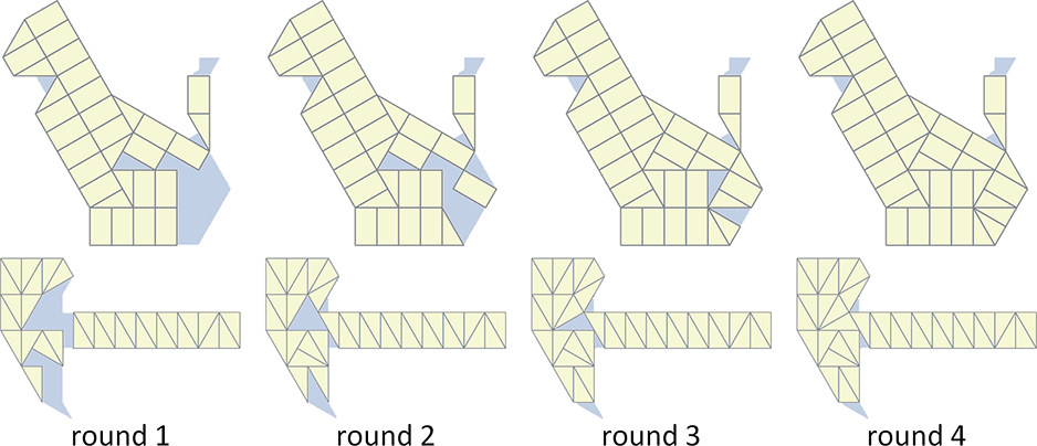
Figure 12. Running examples of using Algorithm 1 to tile the Cat and Hammer shapes. Note that the tiling process usually finishes in one/two rounds; we intentionally pick these two cases with more rounds for illustration. Also, we depict the union of all candidate tile locations in blue under the tiling solutions as a means to visualize the holes and gaps in the results.

Step two: tiling using a trained TilinGNN model

From each $\mathcal{P}$ obtained in step one, we construct adjacency graph $\mathcal{G}$ and its associated network inputs $\{\mathbf{v}_{i}\}$ and $\{\mathbf{e}_{j}\}$, and apply the TilinGNN trained on $\mathcal{T}$ to produce a probability vector on the candidate tile locations in $\mathcal{P}$. Next, we sort the candidate tile locations by the probabilities, and select them in descending order of the probability values. If the next selected tile conflicts (overlaps) with any chosen tile, we stop the selection, create a new (partial) adjacency graph for the remaining candidate tile locations, and start another round of tiling with the trained TilinGNN on the new graph; see Figure 3(c).

Algorithm 1 gives the overall tiling procedure. Very different from the traditional search tools, its running time is roughly linear to the number of nodes in $\mathcal{G}$, so it usually finishes in less than a minute in our experiments. Particularly, the inner loop adopts a probabilistic selection mechanism inspired by the acceptance probability model in general simulated annealing methods (Cagan et al., 1998) to accept tile candidates, so Algorithm 1 has the chance of producing different tiling solutions in different runs. This strategy helps to increase the tiling diversity and avoid holes in the results. Note also that since the network output is already of good quality (see the rightmost result in Figure 11), we usually need only a few (one to two) rounds of tiling in Algorithm 1; see Figure 12 for two typical results with more steps. Note that when we present our tiling solutions (started from Figure 12), we show the 2D region covered by the union of all candidate tile locations in blue color under the tiling solutions for better visualization of the holes and gaps in the results.

Discussion

At the beginning of this research, we attempted to achieve end-to-end training by trying to formulate the loss on Algorithm 1’s output. However, since we cannot directly compute the gradients on such binarized outputs, we thus make use of Algorithm 1 to interpret the outputs of TilinGNN instead.

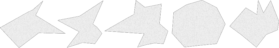
Figure 13. Random shapes (randomly picked from the 12,000 random shape set) we employed for cropping the superset of the candidate tile locations.

6. Results and Experiments

6.1. Implementation Details

We implemented TilinGNN in Python 3.7 using PyTorch (Paszke et al., 2019). We employed Numpy (Oliphant, 2019) to manipulate the arrays and their computations, and Shapely (Gillies et al., 2019) for geometric computations such as collision detection.

Training data preparation.

For each tile set, we pre-computed its superset, i.e., a set of candidate tile locations. Table 1 reports the tile set statistics, in which we sort the table rows by the tile set complexity estimated by the mean degree of graph nodes, i.e., $\frac{2(\left|\mathcal{E}_{\text{ovl}}\right|+\left|\mathcal{E}_{\text{nbr}}\right|)}{\left|\mathcal{V}\right|}$. On the other hand, we prepared 12,000 random shapes for cropping the superset (see Figure 3(b) for how these shapes are used), and randomly divided them into a training set (10,000) and a validation set (2,000). So, one epoch in network training takes 10,000 iterations with the shapes in the training set. To produce a random shape, we randomized its number of vertices in range $\{3,...,20\}$ and its size in range $[0.3,0.8]$, then constructed the shape by randomizing its vertex coordinates. Further, we discarded and re-generated a shape, if it contains any self-intersection. Figure 13 shows some of the random shapes (randomly picked from the 12,000 set), showing that our training process considers both convex and concave shapes.

Table 1. Tile set statistics. From left to right, for each tile set, we show its tile types, number of candidate tile locations in its superset, number of overlap edges ($\left|\mathcal{E}_{\text{ovl}}\right|$), number of neighbor edges ($\left|\mathcal{E}_{\text{nbr}}\right|$), and mean degree of graph nodes ($\frac{2(\left|\mathcal{E}_{\text{ovl}}\right|+\left|\mathcal{E}_{\text{nbr}}\right|)}{\left|\mathcal{V}\right|}$) in its adjacency graph, batch size in network training, training time, and test time (for 20 runs).

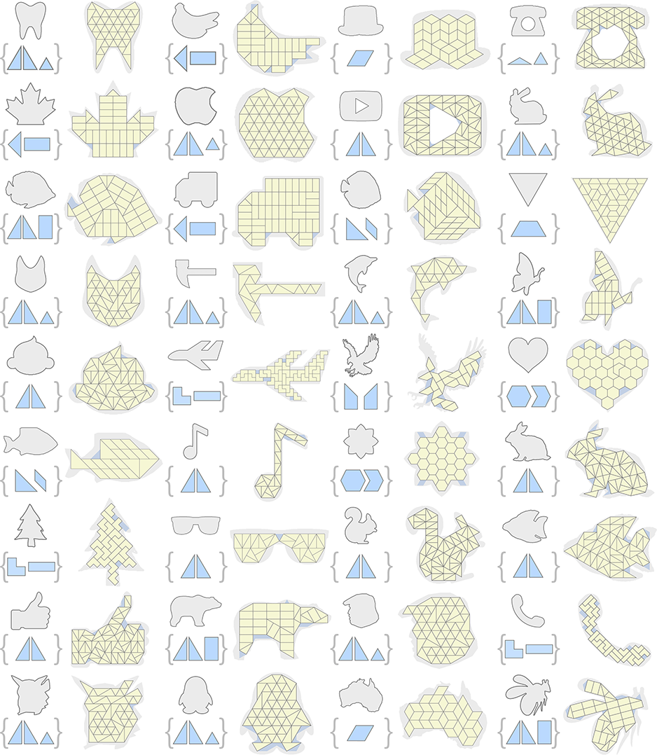
Figure 14. A gallery, showcasing the tiling solutions produced by our learn-to-tile approach on 36 different shapes. Under each tiling solution, we show the original input shape in gray and the region covered by the union of all the candidate tile locations (inside the input shape) in blue, as references.

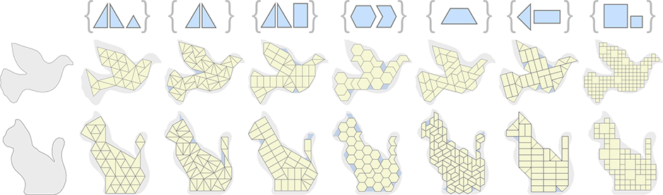
Figure 15. Using our approach to tile the same shape (Dove and Cat) using different tile sets.

Network training.

We trained the TilinGNN model on an NVidia Titan Xp GPU using the Adam optimizer (Kingma and Ba, 2015) with learning rate $10^{-3}$, and ended the training, if the loss stopped to reduce. Overall, it took one to five days to train a model for 20 to 80 epochs. See Table 1 for the training time and batch size.

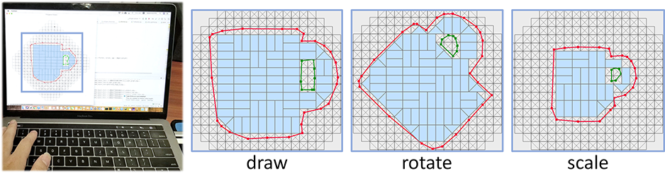
Figure 16. We provide an interactive interface for tiling design, in which we can draw/load a shape, modify it, and preview the tiling solutions.

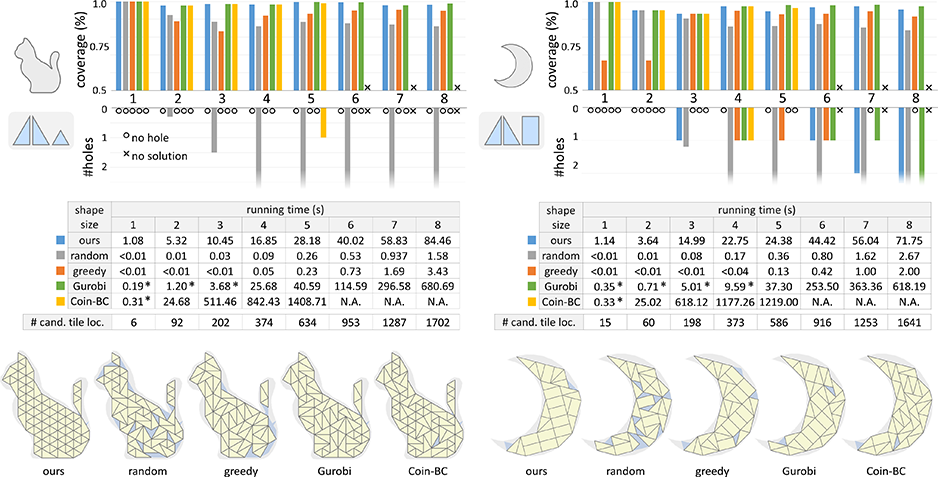
Figure 17. Comparing the performance (tiling coverage, number of holes, and running time) of our method with four alternatives on tiling the Cat and Moon shapes for eight different shape sizes. Note that “# cand. tile loc.” denotes the number of candidate tile locations (solution space). The results here show that our method consistently outperforms others (see Section 6.3 for details), and its running time increases roughly linearly with the number of candidate tile locations. On the bottom, we show tiling solutions produced by the five methods for Cat of shape size five (left) and Moon of shape size four (right).

Tiling generation.

We compiled a set of 107 silhouette images as test shapes. These images were collected by Internet image search and from two public data sets: the MPEG-7 data set (Latecki et al., 2000) and animal shapes from (Bai et al., 2009). Here, we selected the shapes that (i) have distinctive shape features and (ii) do not possess delicate structures such as long and thin tails.

Then, we ran Algorithm 1 on a workstation with 16 CPUs and 125 GB memory to produce tilings on these test shapes. Since our tiling problem has multiple objectives, we may not always avoid holes when putting more emphasis on maximizing the tiling coverage. Thanks to the performance of TilinGNN, we are able to quickly run the tiling procedure multiple times (20 times, in practice), and take the tiling solution with a larger tiling coverage; if multiple results produce the same coverage area, we select the one with a larger total length of contacting edge segments based on loss term $L_{\text{e}}$ (see Section 5.3). Also, we can run multiple threads of the tiling procedure in parallel for better performance. See again Table 1 for the test time performance with different tile sets.

6.2. Tiling solutions

Figure 14 presents a gallery, showcasing tiling solutions produced on 36 different shapes by our learn-to-tile approach. These shapes have different sizes, convexity, and topologies. The average time for our approach to produce these tilings is only 23.5 seconds. Note that all tiling solutions presented in the paper are produced by Algorithm 1, without any post refinement.

Tiling with different tile sets.

Also, we employ tilinGNN models trained on different tile sets to tile the same shape, so as to explore the robustness of our method to variations in tile set. Figure 15 shows two sets of results on tiling the Dove and Cat shapes using seven different tile sets. Our approach can generate interesting tiling solutions for the shapes and reproduced some featured regions using different tile arrangements; see particularly the wings of the different Doves and the tail of the different Cats for examples.

Interactive interface.

Given a shape to tile, if we scale or modify its contour, the tiling solutions will likely change. We provide an interactive interface for loading or drawing a shape and interactively transforming or editing the shape’s contour; see Figure 16. Since the contour is fixed on the tile set’s superset by manual actions on the interface, we can skip step 1 in the tiling procedure (see Section 5.4) and provide a preview of the tiling in one to three seconds, depending on the number of candidate tile locations in the contour. Please see our supplemental video for a demonstration.

Mosaic-style tiling of large regions.

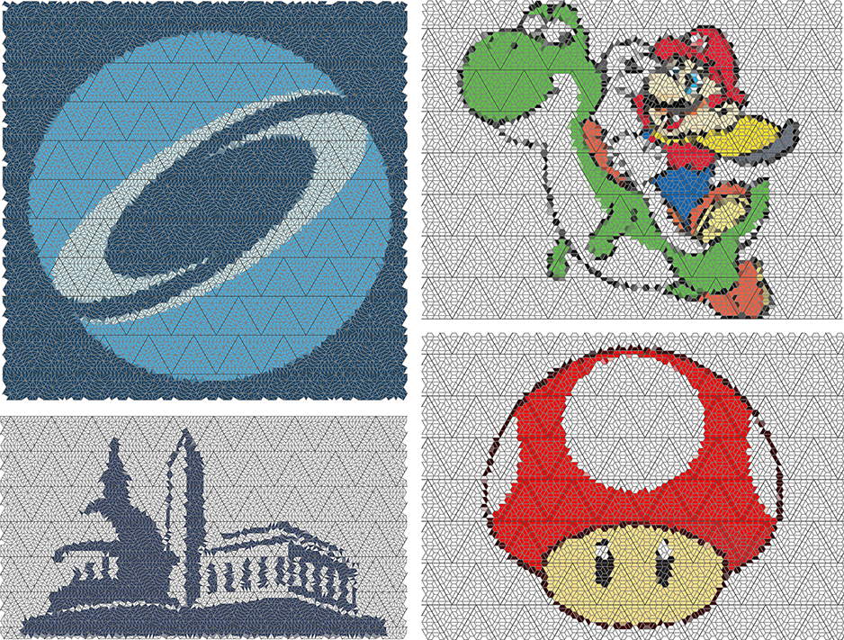
Figure 23. Large mosaic-style tilings produced by subdividing the 2D plane into triangular super-tiles (shown with slightly darker boundaries), employing TilinGNN to tile each super-tile, selecting all tiles lying entirely inside the input image, and assigning a single color from the image to each generated tile.

To produce larger tilings, we can subdivide the domain to be tiled into moderately sized “super-tiles” and apply TilinGNN to tile each super-tile with exact conformation to its boundary. Then, by cropping the tiled region using the input image (i.e., selecting all tiles which lie entirely inside the image boundary) and applying the colors from the image, we can produce mosaic-style tilings, as shown in Figure 23.

Note.

Due to our problem formulation, the cropping process keeps only the candidate tile locations that are fully inside the given 2D shape (see Figure 3(b)). In fact, it is possible to slightly modify our implementation, such that we can relax this restriction and consider candidate tile locations that are partially outside the given 2D shape. Such a modification may help to avoid holes and lead to less jagged boundaries in the generated tiling solutions.

6.3. Evaluations

Comparison with alternative approaches.

We compared our method with four alternatives. The first two are (i) a random search framework that uses Algorithm 1 but replaces the TilinGNN output probabilities with random values in $[0,1]$; and (ii) a greedy strategy that follows existing shape packing methods (e.g., (Kwan et al., 2016)) to iteratively select the tile that shares the longest boundary with the current partial tiling solution. Besides, we employed two state-of-the-art integer programming solvers: (iii) a specialized integer programming solver, Gurobi (2020), which has been shown to perform fast in many combinatorial optimization problems (Luo et al., 2015; Peng et al., 2019; Wu et al., 2018); and (iv) a branch & cut mixed-integer solver (Coin-BC) (2018). To employ them, we formulate our problem using a constraint modeling language, Minizinc (csp, 1999), in which we model the selection of each node as a binary variable, set the tile overlaps as hard constraints, and define an objective function (similar to $L_{a}$ and $L_{e}$ in Section 5.3 but without logarithms) to maximize the tiling coverage and total length of shared edge segments. See supplementary material part B for the code.

Figure 17 reports the comparison results on tiling two different shapes: the percentage of tiling coverage and number of holes (top), running times (middle), and visual comparisons (bottom), where we tile the input shapes for eight different sizes (20% to 90% of the tile set’s superset). For each result (5 methods $\times$ 2 shapes $\times$ 8 sizes), we run the method ten times and take the average. Also, to sense the size of the search space, we provide the number of candidate tile locations per case on the bottom row of the figure tables.

The random strategy, in fact, serves as a control for revealing if TilinGNN is helpful to produce better tilings. Comparing random’s (grey) with ours (blue) in Figure 17, we can see that our approach produces tilings consistently with larger coverage and fewer (or no) holes. Hence, the probability outputs from TilinGNN help improve the tiling solutions. On the other hand, the greedy strategy (orange) is fast and often produces reasonable solutions. However, it relies on a local heuristic, so it cannot produce high tiling coverage.

For Gurobi (green) and Coin-BC (yellow), they are designed for solving discrete combinatorial optimization problems, essentially search problems, meaning that they have to iteratively explore and prune the solution space using strategies such as tree search pruning and the cutting plane method. In practice, they progressively output feasible solutions of high objective values, and do not stop until they find the optimal solutions (after exploring the entire search space with certain pruning). Hence, for a fair comparison with them, we can either restrict their running times to be the same as ours then compare the quality of the tiling solutions, or stop them when they produce tiling solutions of similar/better quality (coverage) as ours then we can compare the running times. For the former strategy, we found that these solvers are only capable of producing tiling solutions for smaller problems (marked with asterisks in the figure tables). Therefore, we took the latter strategy and stop these solvers based on quality. However, for Coin-BC, we found that for some larger problems, it could not produce tiling solutions even running for a long time, so we stop it if it runs 50 times more than our method (marked by N.A. in the figure tables). Overall, from the results shown in Figure 17, we can see that Gurobi and Coin-BC can produce plausible solutions, but they require much longer running time than ours, especially for larger problems. As for our method, its running time increases roughly linearly with the number of candidate tile locations, as shown in Figure 17.

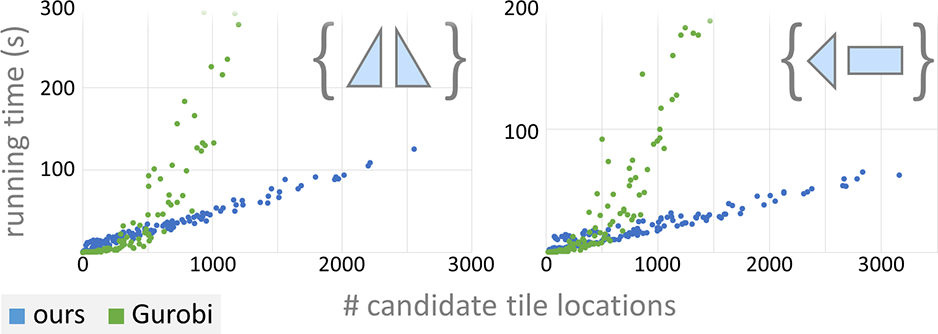
Figure 18. Linearity test. These scatterplots show the running time of our method (blue) and Gurobi (green) for tiling 20 shapes of varying sizes. The plots reveal the running-time linearity of our method with respect to the number of candidate tile locations, while Gurobi grows much faster.

Running time analysis.

Next, we explore the running time of our method and also the Gurobi solver by using them to solve 320 tiling problems: 20 shapes $\times$ 8 sizes $\times$ 2 tile sets. Here, we measured the time taken by each method to generate each result and recorded the associated numbers of candidate tile locations. Same as the previous experiment, we stop Gurobi from running if it produces tiling solutions of similar or better quality as ours. The two scatterplots (for the two different tile sets) shown in Figure 18 report all the numbers, revealing that the time taken by our method increases roughly linearly with the number of candidate tile locations, while the running time of Gurobi grows much faster. For our method, the small fluctuations between results (sample points in the plots) of similar number of candidate tile locations are due to the number of rounds that the tiling procedure took. The number of rounds is usually one or two, but having more than that would suddenly increase the overall running time. For Gurobi, while it solves small-scale problems (with less than $500$ candidate tile locations) quickly, it does not scale well for larger problems.

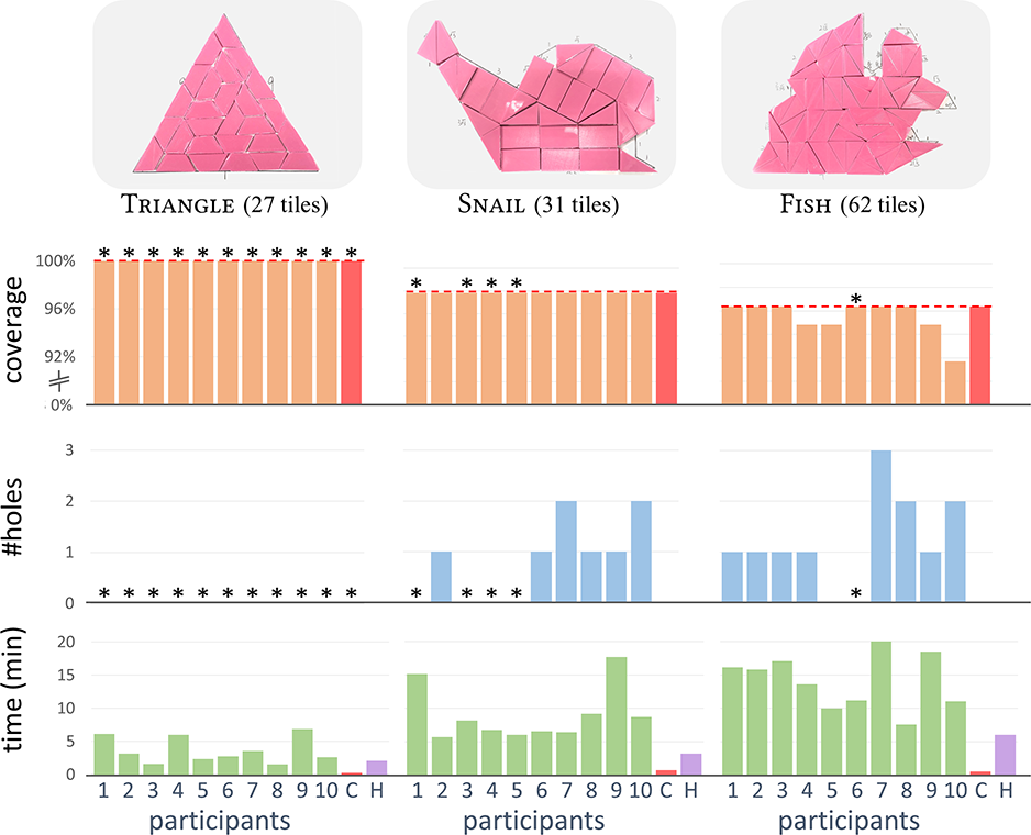
Figure 19. Exploring human performance. We recruited 10 participants to solve three tiling problems (top) and measured their performance in terms of tiling coverage percentage, number of holes, and time spent. Note that the red bars show the performance of our method (denoted by C), whereas the violet bars show the times taken to follow our method’s solutions to manually create the tilings by hands (denoted by H). Also, the asterisks mark the participant solutions that attain the same quality as our method’s.

Human performance.

Next, to explore how humans solve the tiling problems faced by TilinGNN, we picked three tiling solutions produced by TilinGNN with increasing difficulty levels as the tiling problems in this experiment; see Figure 19 (top). For each problem, we 3D-printed the tiles of the tile set, computed the boundary contour of all the candidate tile locations, and further printed out the boundary contour on paper at a scale compatible with the 3D-printed tiles. Hence, the participants could directly manipulate the 3D-printed tiles on the printed paper to work out their solutions.

Overall, we recruited 10 participants who are university students: 3 females & 7 males, aged 22 to 26. When the experiment started, we first introduced the goal of tiling to the participants, i.e., to tile a shape’s interior with maximum area coverage and minimum holes, while not exceeding the shape’s boundary. Hence, they should try to arrange as many tiles as possible in their solutions. Also, we showed them examples of holes, the 2D dimensions of the tiles, and marked the length of each side along the boundary contours on paper. After that, each participant was given at most half an hour to work out their solutions for each tiling problem, in which we recorded the resulting tiling coverage, number of holes, and time spent.

Figure 19 reports the recorded quantities for all the participants and also for our method. The left column shows the simplest case of tiling the Triangle shape, where all participants found the optimal solution with 100% coverage without holes and tile overlaps. The other columns show two harder cases. For Snail, four participants found solutions of same quality as ours: 97.8% coverage and without holes, whereas for Fish, only one participant found a solution of same quality as ours: 96.3% coverage and without holes. For fair comparison on time, we measured the time taken to follow our method’s solutions and manually reproduce the tilings by two hands. On average, the participants took 3.66 mins for Triangle, 9.04 mins for Snail, and 14.13 mins for Fish, while using our method, we took only 0.24 + 1.82 mins for Triangle, 0.70 + 2.51 mins for Snail, and 0.53 + 5.50 mins for Fish. The first numbers are our method’s running times and second numbers are manual tiling times.

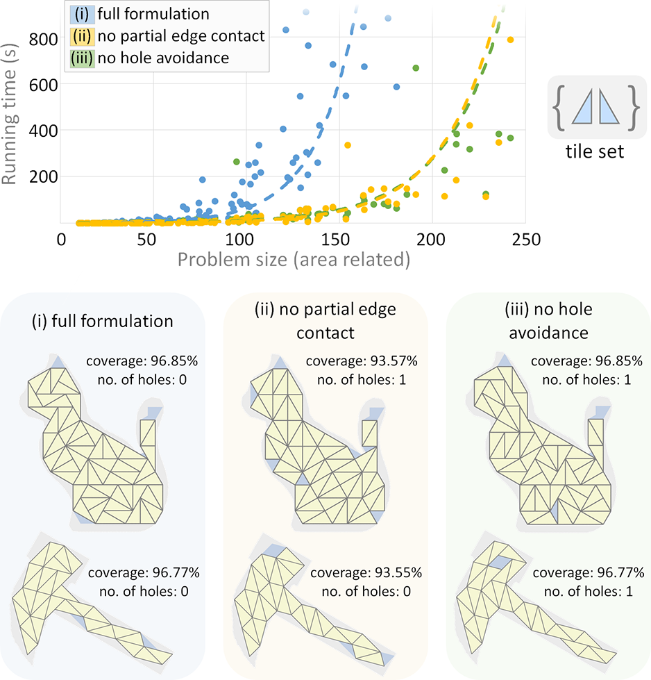
Figure 20. Exploring the computational complexity of considering partial edge contacts between tiles (setting (ii)) and explicit hole avoidance (setting (iii)). Top: scatterplots show the relationship between the running time and problem size for various settings, including the full formulation (setting (i)); comparing the plots for settings (ii) and (iii) against setting (i), we can see that our full formulation is more tedious to compute with, for not so small problem size, thereby revealing the complexity of partial edge contacts and explicit hole avoidance. Bottom: some of the associated tiling solutions.

Complexity: partial edge contacts and hole avoidance.

To explore the computational complexity of considering partial edge contacts (T-junctions) between adjacent tiles and explicit hole avoidance in our formulation, we conducted an experiment with the following three different settings: (i) our full formulation; (ii) our full formulation without candidate tile locations connected with partial edge contacts; and (iii) our full formulation without an $L_{e}$ term for explicitly avoiding holes in the tiling solutions. In detail, we employed the 20 shapes of 8 different sizes as before, and used Gurobi (2020) to search for tiling solutions in each case and setting. Note that we employed Gurobi in this experiment because it can explore the entire search space and find optimal solutions, given sufficient time. By this means, we can sense the complexity of different settings.

Figure 20 (top) presents scatterplots that reveal the relationship between running time and problem size for each setting, whereas Figure 20 (bottom) presents some of the associated tiling solutions. Note, for a fair comparison between settings with and without partial edge contacts, we do not take the number of candidate tile locations as the problem size but use the area covered by the cropped superset, where a single triangle tile is said to have one unit area (see Figure 20 (top) for the tile set). From the plots shown on top of the figure, we can see that if we do not consider partial edge contacts (setting (ii)) or do not explicitly avoid holes (setting (iii)), the running time would decrease significantly for not-so-small problems of same problem size (x-axis), meaning that if we consider partial edge contacts (settings (i) vs. (ii)) or explicitly avoid holes (settings (i) vs. (iii)), Gurobi would require more time in the search and the computation would become more tedious. Also, we use the exponential trendline tool in Excel to fit the dashed lines shown in the plots for each of the three settings to further reveal the relationship between running time and problem size in each setting.

Table 2. Network and loss analysis. Performance (tiling coverage %) of TilinGNN re-trained for various situations of ablating or modifying the network architecture and loss function. Comparing with the re-trained models, the full method (bottom right) consistently achieves better performance.

6.4. Network Analysis

In the following, we present analysis on various aspects of our method by re-training TilinGNN on two different tile sets and applying the re-trained models to tile 20 test shapes, each having three different sizes, i.e., $30\%$, $50\%$, and $80\%$ of a tile set’s superset.

(i) Network architecture analysis.

To evaluate the architecture design of TilinGNN, we removed from it the following network components, one at a time, and re-trained new TilinGNN models:

• no overlap branch, by removing all overlap aggregation modules and all element-wise products at the end of each feature aggregation layer (see Figure 9);

• no edge labels, by setting all elements in $\{\mathbf{e}_{j}\}$ to one;

• no residual connections, by removing the residual connection in both the neighbor and overlap aggregation modules (see Section 5.2 and Figure 10);

• no skip connections, by interpreting only the latent feature of the final layer, i.e., by taking $\mathbf{F}^{L}$ as $\mathcal{F}$ without $\mathbf{F}^{0}$ to $\mathbf{F}^{L-1}$;

• setting network depth $L=10$, which is the number of feature aggregation layers (see Figure 9); and

• using the edge-conditioned convolution layer not only in the neighbor aggregation module but also in the overlap aggregation module (see Section 5.2) by using all-one vectors as the input features and replacing Eq.(2) with Eq.(1) in the overlap aggregation module.

(ii) Loss analysis.

Besides, we re-trained TilinGNN models for the following four situations to analyze the loss function design:

• removing $L_{\text{a}}$, $L_{\text{o}}$, or $L_{\text{e}}$ from the overall loss; and

• summing the three loss terms ($L_{\text{a}}+L_{\text{o}}+L_{\text{e}}$) rather than multiplying them as the overall loss.

For comparison purpose, we compute the percentage coverage of each tiling solution, and consider the average percentage over the test shapes for each re-trained TilinGNN model as its performance. Table 2 reports the performance for all the above ten cases, including also the performance of our full method. Comparing the numbers shown in the table, we can see that if we ablate TilinGNN by removing the overlap branch, by removing the edge labels, etc., or by modifying its architecture or loss function, the tiling performance drops. This reveals the contributions of individual network components and the loss function design to the full method.

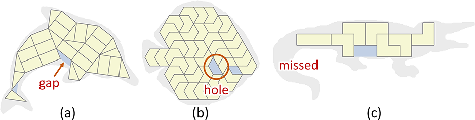
Figure 21. Potential issues in our tiling solutions.

Figure 22. The example square-triangle tile set (Wikipedia, 2020) does not induce a periodic grid for the candidate tile locations. In the recursive tile enumeration, most newly generated candidate tiles do not coincide with the existing ones, leading to an unbounded expansion of candidate tiles.

7. Conclusion

We presented the first deep-learning-based approach to generate non-periodic tilings on given 2D shapes. Overall, our approach has three main contributions. First, we model tiling as a graph problem with nodes and edges representing the candidate tile locations and tile connectivity, so we can adopt a graph neural network to solve the problem by learning features to predict probabilities for tile placements. Second, we design TilinGNN, a two-branch graph convolutional neural network model with the neighbor and overlap aggregation modules to progressively aggregate features along graph nodes for producing tilings with maximized coverage, while avoiding holes and tile overlaps. Third, we formulate these criteria as loss terms defined on the network outputs, so we do not require manual preparation of ground-truth tilings, and the network training can be self-supervised. Our method works on many different forms of tile sets and allows contacts at partial segments.

We performed various experiments to evaluate the quality of our approach, and presented a variety of tiling results to demonstrate the possibility of using a neural network to learn to produce tilings. Experimentally, the running time of our network is roughly linear to the number of candidate tile locations, which far exceeds the performance of conventional combinatorial search tools.

Limitations.

As a first attempt to generate tilings by machine learning, our method still has several limitations. First, as explained earlier in Section 4.1, TilinGNN is a selection network that learns to select from a finite set of candidate tile locations, so we consider tile sets that the induced candidate tile locations form periodic grids, e.g., see the superset in Figure 3(a). Hence, TilinGNN cannot deal with all kinds of tile sets, e.g., the Penrose tile set and the square-triangle tile set shown in Figure 22. Also, it is unclear how the network can effectively enforce symmetries in the tiling. We did attempt to include symmetry as a loss term, but network training became an issue, where the loss did not converge. In general, compared to existing IP solvers such as Gurobi, our method lacks the ability to impose hard constraints or tweak the objective functions.

Furthermore, results from TilinGNN may not always avoid gaps (see Figure 21 (a)) and holes (see Figure 21 (b)), due to the multi-objective goal, which also needs to address the tiling coverage and overlap avoidance. Also, the tiling results may miss shape structures that are typically thin (see Figure 21 (c)), if the shape does not fully cover surrounding candidate tile locations in the cropping. At last, from a computational standpoint, the scalability of our current implementation, or the maximum problem size that can be solved, is limited by the available GPU memory.

Discussion.

Combinatorial optimization is often a challenging but necessary problem to face in computer graphics research, whenever we have discrete options to choose in our problem. In this work, we present a novel approach for tiling generation, where we demonstrate that discrete options, together with their constraints, can be formulated as a graph problem. Consequently, we can then adopt and formulate a graph neural network to work on the problem. Our overall framework is general and has great potential for solving other combinatorial problems. Having said that, if we can connect the discrete options into a graph structure and model the constraints in the graph, we can then design features to be produced and aggregated at the nodes and along the edges for graph learning. Taking the hybrid mesh problem (Peng et al., 2018) as an example, to decide whether to use a triangle or a quad at any local area is a discrete option, and such a local option affects the other local options that surround it. Hence, if we can model the relations between local options into a graph, a graph learning model may be adopted to learn to create such mesh. Besides, computational assembly problems (Luo et al., 2012; Deuss et al., 2014; Xu et al., 2019c) often involve discrete options, in which we are strongly interested in exploring machine learning approaches to solving these problems.

- (1)
- csp (1999) 1999. CSPLib: A problem library for constraints. Available from http://www.csplib.org.
- Abe et al. (2019) Kenshin Abe, Zijian Xu, Issei Sato, and Masashi Sugiyama. 2019. Solving NP-Hard Problems on Graphs by Reinforcement Learning without Domain Knowledge. arXiv preprint arXiv:1905.11623 (2019).
- Bai et al. (2009) Xiang Bai, Wenyu Liu, and Zhuowen Tu. 2009. Integrating contour and skeleton for shape classification. In International Conference on Computer Vision Workshops. IEEE, 360–367.
- Bau et al. (2019) David Bau, Hendrik Strobelt, William Peebles, Jonas Wulff, Bolei Zhou, Jun-Yan Zhu, and Antonio Torralba. 2019. Semantic Photo Manipulation with a Generative Image Prior. ACM Transactions on Graphics (SIGGRAPH) 38, 4, Article 59 (2019).
- Bello et al. (2016) Irwan Bello, Hieu Pham, Quoc V Le, Mohammad Norouzi, and Samy Bengio. 2016. Neural combinatorial optimization with reinforcement learning. arXiv preprint arXiv:1611.09940 (2016).
- Cagan et al. (1998) Jonathan Cagan, Drew Degentesh, and Su Yin. 1998. A simulated annealing-based algorithm using hierarchical models for general three-dimensional component layout. Computer-aided design 30, 10 (1998), 781–790.
- Chen et al. (2017) Weikai Chen, Yuexin Ma, Sylvain Lefebvre, Shiqing Xin, Jonàs Martínez, and Wenping Wang. 2017. Fabricable Tile Decors. ACM Transactions on Graphics (SIGGRAPH Asia) 36, 6, Article 175 (2017).
- Chen et al. (2018) Xuelin Chen, Honghua Li, Chi-Wing Fu, Hao Zhang, Daniel Cohen-Or, and Baoquan Chen. 2018. 3D Fabrication with Universal Building Blocks and Pyramidal Shells. ACM Transactions on Graphics (SIGGRAPH Asia) 37, 6, Article 189 (2018).
- Cohen et al. (2003) Michael F. Cohen, Jonathan Shade, Stefan Hiller, and Oliver Deussen. 2003. Wang Tiles for Image and Texture Generation. ACM Transactions on Graphics (SIGGRAPH) 22, 3 (2003), 287–294.
- Dai et al. (2017) Hanjun Dai, Elias B. Khalil, Yuyu Zhang, Bistra Dilkina, and Le Song. 2017. Learning combinatorial optimization algorithms over graphs. In Advances in Neural Information Processing Systems. 6349–6359.
- Deuss et al. (2014) Mario Deuss, Daniele Panozzo, Emily Whiting, Yang Liu, Philippe Block, Olga Sorkine-Hornung, and Mark Pauly. 2014. Assembling Self-Supporting Structures. ACM Transactions on Graphics (SIGGRAPH) 33, 6, Article 214 (2014).
- Duncan et al. (2017) Noah Duncan, Lap-Fai Yu, Sai-Kit Yeung, and Demetri Terzopoulos. 2017. Approximate Dissections. ACM Transactions on Graphics (SIGGRAPH Asia) 36, 6, Article 182 (2017).
- Eigensatz et al. (2010) Michael Eigensatz, Martin Kilian, Alexander Schiftner, Niloy Mitra, Helmut Pottmann, and Mark Pauly. 2010. Paneling Architectural Freeform Surfaces. ACM Transactions on Graphics (SIGGRAPH) 29, 3, Article 45 (2010).
- Forrest et al. (2018) John J. Forrest, Lou Hafer, and Joao P. Goncalves. 2018. coin-or/Cbc: Version 2.9.9. https://github.com/coin-or/Cbc
- Fu et al. (2010) Chi-Wing Fu, Chi-Fu Lai, Ying He, and Daniel Cohen-Or. 2010. K-set Tilable Surfaces. ACM Transactions on Graphics (SIGGRAPH) 29, 3, Article 44 (2010).
- Gao et al. (2019) Lin Gao, Jie Yang, Tong Wu, Yu-Jie Yuan, Hongbo Fu, Yu-Kun Lai, and Hao Zhang. 2019. SDM-NET: deep generative network for structured deformable mesh. ACM Transactions on Graphics (SIGGRAPH Asia) 38, 6, Article 243 (2019).
- Gillies et al. (2019) Sean Gillies et al. 2019. Shapely: Manipulation and Analysis of Geometric Objects. Available from https://github.com/Toblerity/Shapely.
- Grünbaum and Shephard (1986) Branko Grünbaum and G. C. Shephard. 1986. Tilings and patterns. W. H. Freeman & Co.
- Gurobi Optimization (2020) LLC Gurobi Optimization. 2020. Gurobi Optimizer Reference Manual. http://www.gurobi.com
- Hanocka et al. (2019) Rana Hanocka, Amir Hertz, Noa Fish, Raja Giryes, Shachar Fleishman, and Daniel Cohen-Or. 2019. MeshCNN: a network with an edge. ACM Transactions on Graphics (SIGGRAPH) 38, 4, Article 90 (2019).
- Hausner (2001) Alejo Hausner. 2001. Simulating decorative mosaics. In Proc. of SIGGRAPH. 573–580.
- He et al. (2016) Kaiming He, Xiangyu Zhang, Shaoqing Ren, and Jian Sun. 2016. Deep residual learning for image recognition. In IEEE Conf. on Computer Vision and Pattern Recognition. 770–778.
- Hiller et al. (2003) Stefan Hiller, Heino Hellwig, and Oliver Deussen. 2003. Beyond Stippling - Methods for Distributing Objects on the Plane. Computer Graphics Forum (Eurographics) 22, 3 (2003), 515–522.
- Huang et al. (2011) Hua Huang, Lei Zhang, and Hong-Chao Zhang. 2011. Arcimboldo-like Collage Using Internet Images. ACM Transactions on Graphics (SIGGRAPH Asia) 30, 6, Article 155 (2011).
- Jamriška et al. (2019) Ondřej Jamriška, Šárka Sochorová, Ondřej Texler, Michal Lukáč, Jakub Fišer, Jingwan Lu, Eli Shechtman, and Daniel Sýkora. 2019. Stylizing Video by Example. ACM Transactions on Graphics (SIGGRAPH) 38, 4, Article 107 (2019).
- Kaplan (2009) Craig S. Kaplan. 2009. Introductory Tiling Theory for Computer Graphics. Morgan & Claypool.
- Kaplan and Salesin (2000) Craig S. Kaplan and David H. Salesin. 2000. Escherization. In Proc. of SIGGRAPH. 499–510.
- Kaplan and Salesin (2004) Craig S. Kaplan and David H. Salesin. 2004. Islamic Star Patterns in Absolute Geometry. ACM Transactions on Graphics 23, 2 (2004), 97–119.
- Kim and Pellacini (2002) Junhwan Kim and Fabio Pellacini. 2002. Jigsaw Image Mosaics. ACM Transactions on Graphics (SIGGRAPH) 21, 3 (2002), 657–664.
- Kingma and Ba (2015) Diederik P. Kingma and Jimmy Ba. 2015. Adam: A method for stochastic optimization. In International Conference for Learning Representations.
- Kopf et al. (2006) Johannes Kopf, Daniel Cohen-Or, Oliver Deussen, and Dani Lischinski. 2006. Recursive Wang Tiles for Real-Time Blue Noise. ACM Transactions on Graphics (SIGGRAPH) 25, 3 (2006), 509–518.
- Kwan et al. (2016) Kin Chung Kwan, Lok Tsun Sinn, Chu Han, Tien-Tsin Wong, and Chi-Wing Fu. 2016. Pyramid of Arclength Descriptor for Generating Collage of Shapes. ACM Transactions on Graphics (SIGGRAPH Asia) 35, 6, Article 229 (2016).
- Latecki et al. (2000) Longin Jan Latecki, Rolf Lakamper, and T. Eckhardt. 2000. Shape descriptors for non-rigid shapes with a single closed contour. In IEEE Conf. on Computer Vision and Pattern Recognition. 424–429.
- Leimkühler et al. (2019) Thomas Leimkühler, Gurprit Singh, Karol Myszkowski, Hans-Peter Seidel, and Tobias Ritschel. 2019. Deep point correlation design. ACM Transactions on Graphics (SIGGRAPH Asia) 38, 6, Article 226 (2019).
- Lemos et al. (2019) Henrique Lemos, Marcelo Prates, Pedro Avelar, and Luís Lamb. 2019. Graph Colouring Meets Deep Learning: Effective Graph Neural Network Models for Combinatorial Problems. In International Conference on Tools with Artificial Intelligence. 879–885.
- Li et al. (2017) Jun Li, Kai Xu, Siddhartha Chaudhuri, Ersin Yumer, Hao Zhang, and Leonidas J. Guibas. 2017. GRASS: Generative Recursive Autoencoders for Shape Structures. ACM Transactions on Graphics (SIGGRAPH) 36, 4, Article 52 (2017).
- Li et al. (2019) Manyi Li, Akshay Gadi Patil, Kai Xu, Siddhartha Chaudhuri, Owais Khan, Ariel Shamir, Changhe Tu, Baoquan Chen, Daniel Cohen-Or, and Hao Zhang. 2019. GRAINS: Generative Recursive Autoencoders for Indoor Scenes. ACM Transactions on Graphics 38, 2, Article 12 (2019).
- Li et al. (2018b) Shuhua Li, Ali Mahdavi-Amiri, Ruizhen Hu, Han Liu, Changqing Zou, Oliver Van Kaick, Xiuping Liu, Hui Huang, and Hao Zhang. 2018b. Construction and Fabrication of Reversible Shape Transforms. ACM Transactions on Graphics (SIGGRAPH Asia) 37, 6, Article 190 (2018).
- Li et al. (2018a) Zhuwen Li, Qifeng Chen, and Vladlen Koltun. 2018a. Combinatorial optimization with graph convolutional networks and guided tree search. In Advances in Neural Information Processing Systems. 539–548.
- Lien and Amato (2004) Jyh-Ming Lien and Nancy M. Amato. 2004. Approximate Convex Decomposition of Polygons. Computational Geometry: Theory & Applications (2004).
- Luo et al. (2012) Linjie Luo, Ilya Baran, Szymon Rusinkiewicz, and Wojciech Matusik. 2012. Chopper: Partitioning Models into 3D-Printable Parts. ACM Transactions on Graphics (SIGGRAPH Asia) 31, 6, Article 129 (2012).
- Luo et al. (2015) Sheng-Jie Luo, Yonghao Yue, Chun-Kai Huang, Yu-Huan Chung, Sei Imai, Tomoyuki Nishita, and Bing-Yu Chen. 2015. Legolization: optimizing LEGO designs. ACM Transactions on Graphics (SIGGRAPH Asia) 34, 6, Article 222 (2015).
- Mo et al. (2019) Kaichun Mo, Paul Guerrero, Li Yi, Hao Su, Peter Wonka, Niloy Mitra, and Leonidas J. Guibas. 2019. StructureNet: Hierarchical Graph Networks for 3D Shape Generation. ACM Transactions on Graphics (SIGGRAPH Asia) 38, 6, Article 242 (2019).
- Moore and Robson (2001) Cristopher Moore and John Michael Robson. 2001. Hard Tiling Problems with Simple Tiles. Discrete & Computational Geometry 26 (2001), 573–590.
- Oliphant (2019) Travis Oliphant. 2019. NumPy: A Guide to NumPy. Available from http://www.numpy.org/.
- Ostromoukhov (2007) Victor Ostromoukhov. 2007. Sampling with Polyominoes. ACM Transactions on Graphics (SIGGRAPH) 26, 3, Article 78 (2007).
- Paszke et al. (2019) Adam Paszke, Sam Gross, Francisco Massa, Adam Lerer, James Bradbury, Gregory Chanan, Trevor Killeen, Zeming Lin, Natalia Gimelshein, Luca Antiga, Alban Desmaison, Andreas Kopf, Edward Yang, Zachary DeVito, Martin Raison, Alykhan Tejani, Sasank Chilamkurthy, Benoit Steiner, Lu Fang, Junjie Bai, and Soumith Chintala. 2019. PyTorch: An Imperative Style, High-Performance Deep Learning Library. In Advances in Neural Information Processing Systems 32. 8024–8035.
- Peng et al. (2019) Chi-Han Peng, Caigui Jiang, Peter Wonka, and Helmut Pottmann. 2019. Checkerboard patterns with black rectangles. ACM Transactions on Graphics (SIGGRAPH Asia) 38, 6, Article 171 (2019).
- Peng et al. (2018) Chi-Han Peng, Helmut Pottmann, and Peter Wonka. 2018. Designing Patterns Using Triangle-Quad Hybrid Meshes. ACM Transactions on Graphics (SIGGRAPH) 37, 4, Article 107 (2018).
- Peng et al. (2014) Chi-Han Peng, Yong-Liang Yang, and Peter Wonka. 2014. Computing Layouts with Deformable Templates. ACM Transactions on Graphics (SIGGRAPH) 33, 4, Article 99 (2014).
- Reinert et al. (2013) Bernhard Reinert, Tobias Ritschel, and Hans-Peter Seidel. 2013. Interactive by-example design of artistic packing layouts. ACM Transactions on Graphics (SIGGRAPH Asia) 32, 6, Article 218 (2013).
- Saputra et al. (2017) Reza Adhitya Saputra, Craig S. Kaplan, Paul Asente, and Radom’ir Mĕch. 2017. FLOWPAK: Flow-based Ornamental Element Packing. In Graphics Interface. 8–15.
- Silver et al. (2017) David Silver, Julian Schrittwieser, Karen Simonyan, Ioannis Antonoglou, Aja Huang, Arthur Guez, Thomas Hubert, Lucas Baker, Matthew Lai, Adrian Bolton, et al. 2017. Mastering the game of Go without human knowledge. Nature 550, 7676 (2017), 354–359.
- Simonovsky and Komodakis (2017) Martin Simonovsky and Nikos Komodakis. 2017. Dynamic edge-conditioned filters in convolutional neural networks on graphs. In IEEE Conf. on Computer Vision and Pattern Recognition. 3693–3702.
- Singh and Schaefer (2010) Mayank Singh and Scott Schaefer. 2010. Triangle Surfaces with Discrete Equivalence Classes. ACM Transactions on Graphics (SIGGRAPH) 29, 3, Article 46 (2010).
- Skouras et al. (2015) Mélina Skouras, Stelian Coros, Eitan Grinspun, and Bernhard Thomaszewski. 2015. Interactive Surface Design with Interlocking Elements. ACM Transactions on Graphics (SIGGRAPH Asia) 34, 6, Article 224 (2015).
- Smith et al. (2005) Kaleigh Smith, Yunjun Liu, and Allison Klein. 2005. Animosaics. In Proceedings of the 2005 ACM SIGGRAPH/Eurographics symposium on Computer animation. ACM, 201–208.
- Stam (1997) Jos Stam. 1997. Aperiodic Texture Mapping. Tech. Report R046. European Research Consortium for Informatics and Mathematics.
- Sun et al. (2019) Tiancheng Sun, Jonathan T. Barron, Yun-Ta Tsai, Zexiang Xu, Xueming Yu, Graham Fyffe, Christoph Rhemann, Jay Busch, Paul Debevec, and Ravi Ramamoorthi. 2019. Single Image Portrait Relighting. ACM Transactions on Graphics (SIGGRAPH) 38, 4, Article 79 (2019).
- Toenshoff et al. (2019) Jan Toenshoff, Martin Ritzert, Hinrikus Wolf, and Martin Grohe. 2019. Graph Neural Networks for Maximum Constraint Satisfaction. arXiv preprint arXiv:1909.08387 (2019).
- Vinyals et al. (2015) Oriol Vinyals, Meire Fortunato, and Navdeep Jaitly. 2015. Pointer Networks. In Advances in Neural Information Processing Systems. 2692–2700.
- Wang et al. (2019) Kai Wang, Yu-An Lin, Ben Weissmann, Manolis Savva, Angel X. Chang, and Daniel Ritchie. 2019. PlanIT: Planning and Instantiating Indoor Scenes with Relation Graph and Spatial Prior Networks. ACM Transactions on Graphics (SIGGRAPH) 38, 4, Article 132 (2019).
- Wikipedia (2020) Wikipedia. 2020. List of aperiodic sets of tiles — Wikipedia, The Free Encyclopedia. [Online; accessed 29-April-2020].
- Wu et al. (2018) Kui Wu, Xifeng Gao, Zachary Ferguson, Daniele Panozzo, and Cem Yuksel. 2018. Stitch Meshing. ACM Transactions on Graphics (SIGGRAPH) 37, 4, Article 130 (2018).
- Wu et al. (2019) Zonghan Wu, Shirui Pan, Fengwen Chen, Guodong Long, Chengqi Zhang, and Philip S. Yu. 2019. A Comprehensive Survey on Graph Neural Networks. CoRR abs/1901.00596 (2019). arXiv:1901.00596 http://arxiv.org/abs/1901.00596
- Xu et al. (2019c) Hao Xu, Ka-Hei Hui, Chi-Wing Fu, and Hao Zhang. 2019c. Computational LEGO Technic Design. ACM Transactions on Graphics (SIGGRAPH Asia) 38, 6, Article 196 (2019).
- Xu et al. (2019b) Keyulu Xu, Weihua Hu, Jure Leskovec, and Stefanie Jegelka. 2019b. How powerful are graph neural networks?. In International Conference for Learning Representations.
- Xu et al. (2019a) Pengfei Xu, Jiangqiang Ding, Hao Zhang, and Hui Huang. 2019a. Discernible image mosaic with edge-Aware adaptive tiles. 5, 1 (2019), 45–58.
- Yolcu and Póczos (2019) Emre Yolcu and Barnabás Póczos. 2019. Learning Local Search Heuristics for Boolean Satisfiability. In Advances in Neural Information Processing Systems. 7990–8001.