Temporal Logic Trees for Model Checking and Control Synthesis of Uncertain Discrete-time Systems
Abstract
We propose algorithms for performing model checking and control synthesis for discrete-time uncertain systems under linear temporal logic (LTL) specifications. We construct temporal logic trees (TLT) from LTL formulae via reachability analysis. In contrast to automaton-based methods, the construction of the TLT is abstraction-free for infinite systems, that is, we do not construct discrete abstractions of the infinite systems. Moreover, for a given transition system and an LTL formula, we prove that there exist both a universal TLT and an existential TLT via minimal and maximal reachability analysis, respectively. We show that the universal TLT is an underapproximation for the LTL formula and the existential TLT is an overapproximation. We provide sufficient conditions and necessary conditions to verify whether a transition system satisfies an LTL formula by using the TLT approximations. As a major contribution of this work, for a controlled transition system and an LTL formula, we prove that a controlled TLT can be constructed from the LTL formula via control-dependent reachability analysis. Based on the controlled TLT, we design an online control synthesis algorithm, under which a set of feasible control inputs can be generated at each time step. We also prove that this algorithm is recursively feasible. We illustrate the proposed methods for both finite and infinite systems and highlight the generality and online scalability with two simulated examples.
I Introduction
In the recent past the integration of computer science and control theory has promoted the development of new areas such as embedded systems design [1], hybrid systems theory [2], and, more recently, cyber-physical systems [3]. Given a model of a dynamical process and a specification (i.e., a description of desired properties), two fundamental problems arise:
-
•
model checking: automatically verifying whether the behavior of the model satisfies the given specification;
-
•
formal control synthesis: automatically designing controllers (inputs to the system) so that the behavior of the model provably satisfies the given specification.
Both problems are of great interest in disparate and diverse applications, such as robotics, transportation systems, and safety-critical embedded system design. However, they are challenging problems when considering dynamical systems affected by uncertainty, and in particular uncertain infinite (uncountable) systems under complex, temporal logic specifications. In this paper, we provide solutions to the model checking and formal control synthesis problems, for discrete-time uncertain systems under linear temporal logic (LTL) specification.
I-A Related Work
In general, LTL formulae are expressive enough to capture many important properties, e.g., safety (nothing bad will ever happen), liveness (something good will eventually happen), and more complex combinations of Boolean and temporal statements [4].
In the area of formal verification, a dynamical process is by and large modeled as a finite transition system. A typical approach to both model checking and control synthesis for a finite transition system and an LTL formula leverages automata theory. It is known that each LTL formula can be transformed to an equivalent automaton [5]. The model checking problem can be solved by verifying whether the intersection of the trace set of the transition system and the set of accepted languages of the automaton expressing the negation of the LTL formula is empty, or not [4]. The control synthesis problem can be solved by the following steps: (1) translate the LTL formula into a deterministic automaton; (2) build a “product automaton” between the transition system and the obtained automaton; (3) transform the product automaton into a game [6]; (4) solve the game [7, 8, 9]; and (5) map the solution into a control strategy.
In recent years, the study of model checking and control synthesis for dynamical systems with continuous (uncountable) spaces, which extends the standard setup in formal verification, has attracted significant attention within the control community. This has enabled the formal control synthesis for interesting properties, which are more complex than the usual control objectives such as stability and set invariance. In order to adapt automaton-based methods to infinite systems, abstraction plays a central role in both model checking and control synthesis, which entails: (1) to abstract an infinite system to a finite transition system; (2) to conduct automaton-based model checking or control synthesis for the finite transition system; (3) if a solution is found, to map it back to the infinite system; otherwise, to refine the finite transition system and repeat the steps above.
In order to show the correctness of the solution obtained from the abstracted finite system over the infinite system, an equivalence or inclusion relation between the abstracted finite system and the infinite system needs to be established [10]. Relevant notions include (approximate) bisimulations and simulations. These relations and their variants have been explored for systems that are incrementally (input-to-state) stable [11, 12], or systems with similar properties [13]. Recent work [14] shows that the condition of approximate simulation can be relaxed to controlled globally asymptotic or practical stability with respect to a given set for nonlinear systems. We remark that such condition holds for only a small class of systems in practice.
Based on abstractions, the problem of model checking for infinite systems has been studied in [15, 16]. In [15], it is shown that model checking for discrete-time, controllable, linear systems from LTL formulae is decidable through an equivalent finite abstraction. In [16], the authors study the problem of verifying whether a linear system with additive uncertainty from some initial states satisfies a fragment of LTL formulae, which can be transformed to a deterministic Büchi automaton. The key idea is to use a formula-guided method to construct and refine a finite system abstracted from the linear system and guarantee their equivalence. Along the same line, the problem of control synthesis has also been widely studied for linear systems [17], nonlinear systems [18], stochastic systems [19], hybrid systems [20], and stochastic hybrid systems [21]. The applications of control synthesis under LTL specifications include single-robot control in dynamic environments [22], multi-robot control [23], and transportation control [24].
Beyond automata-based methods, alternative attempts have been made for specific model classes. Receding horizon methods are used to design controllers under LTL for deterministic linear systems [25] and uncertain linear systems [26]. The control of Markov decision processes under LTL is considered in [25] and further applied to multi-robot coordination in [27]. Control synthesis for dynamical systems has been extended also to other specifications like signal temporal logic (STL) [28], and probabilistic computational tree logic (PCTL) [29]. Interested readers may refer to the tutorial paper [30] and the book [31] for detailed discussions.
I-B Motivations
Although the last two decades have witnessed a great progress on model checking and control synthesis for infinite systems from both theoretical and practical perspectives, there are some inherent restrictions in the dominant automaton-based methods.
First, abstraction from infinite systems to finite systems suffers from the curse of dimensionality: abstraction techniques usually partition the state space, and transitions are constructed via reachability analysis. The computational complexity increases exponentially with the system dimension. Many works are dedicated to improving the computational efficiency by using overapproximation for (mixed) monotone systems [24], or by exploiting the structure of the uncertainty [21]. However, another issue with abstraction techniques is that only systems with “good properties” (e.g., incremental stability, or smooth dynamics) might admit finite abstractions with guarantees, which limits their generality.
Second, there are few results for handling general LTL formulae when an infinite system comes with uncertainty (e.g., bounded disturbance, or additive noise). In most contributions on control synthesis of uncertain systems, fragments of LTL formulae (e.g., bounded LTL or co-safe LTL) are usually taken into account [32, 33]. As mentioned before, the LTL formulae are defined over infinite trajectories and it is difficult to control uncertainties propagating along such trajectories. This restriction results from conservative over-approximation in the computation of forward reachable sets, which is widely used for abstraction, and which leads to information loss when used with automaton-based methods.
Third, current methods usually lack online scalability. In many applications, full a priori knowledge of a specification cannot be obtained. For example, consider an automated vehicle required to move from some initial position to some destination without colliding into any obstacle (e.g., other vehicles and pedestrians). Since the trajectories of other vehicles and pedestrians cannot be accurately predicted, we cannot in advance define a specification that captures all the possibilities during the navigation process. Thus, offline design of automaton-based methods is significantly restricted.
Finally, the controller obtained from automaton-based methods usually only contains a single control policy. In some applications, e.g., human-in-the-loop control [34, 35], a set of feasible control inputs are needed to provide more degrees of freedom in the actual implementation. For example, [34] studies a control problem where humans are given a higher priority than the automated system in the decision making process. A controller is designed to provide a set of admissible control inputs with enough degrees of freedom to allow the human operator to easily complete the task.
I-C Contributions
Motivated by the above, this paper studies LTL model checking and reachability-based control synthesis for discrete-time uncertain systems. There are many results for reachability analysis on infinite systems [36, 37] and the computation of both forward and backward reachable sets has been widely studied [38, 39, 40]. The connection between STL and reachability analysis is studied in [41], which inspires our work. The main contributions of this paper are three-fold:
(1) We construct tree structures from LTL formulae via reachability analysis over dynamical models. We denote the tree structure as a temporal logic tree (TLT). The connection between TLT and LTL is shown to hold for both uncertain finite and infinite models. The construction of the TLT is abstraction-free for infinite systems and admits online implementation, as demonstrated in Section VI. More specifically, given a system and an LTL formula, we prove that both a universal TLT and an existential TLT can be constructed for the LTL formula via minimal and maximal reachability analysis, respectively (Theorems III.1 and III.2). We also show that the universal TLT is an underapproximation for the LTL formula and the existential TLT is an overapproximation for the LTL formula. Our formulation does not restrict the generality of LTL formulae.
(2) We provide a method for model checking of discrete-time dynamical systems using TLTs. We provide sufficient conditions to verify whether a transition system satisfies an LTL formula by using universal TLTs for under-approximating the satisfaction set, or alternatively using existential TLTs for over-approximating the violation set (Theorem IV.1). Dually, we provide necessary conditions by using existential TLTs for over-approximating the satisfaction set, or alternatively using universal TLTs for under-approximating the violation set (Theorem IV.2).
(3) As a core and novel contribution of this work, we detail an approach for online control synthesis for a controlled transition system to guarantee that the controlled system will satisfy the specified LTL formula. Given a control system and an LTL formula, we construct a controlled TLT (Theorem V.1). Based on the obtained TLT, we design an online control synthesis algorithm, under which a set of feasible control inputs is generated at each time step (Algorithm 3). We prove that this algorithm is recursively feasible (Theorem V.2). We provide applications to show the scalability of our methods.
I-D Organization
The remainder of the paper is organized as follows. In Section II, we define the notion of transition system, recall the problem of reachability analysis, and provide preliminaries on LTL specifications. In Section III, we introduce TLT structures and show how to construct a TLT from a given LTL formula. In Section IV, we solve the LTL model checking problem through the constructed TLT. Section V solves the LTL control synthesis problem. In Section VI, we illustrate the effectiveness of our approaches with two numerical examples. In Section VII, we conclude the paper with a discussion about our work and future directions.
II Preliminaries
This section will first introduce transition systems and then recall reachability analysis and LTL.
II-A Transition System
Definition II.1.
A transition system is a tuple consisting of
-
•
a set of states;
-
•
a transition relation 111Here, the transition relation is not a functional relation, but instead for some state , there may exist two different states and such that and hold. For notational simplicity, we use , rather than . The same claim holds for the controlled transition systems in Section V.;
-
•
a set of initial states;
-
•
a set of atomic propositions;
-
•
a labelling function .
Definition II.2.
A transition system is said to be finite if and .
Definition II.3.
For , the set of direct successors of is defined by .
Definition II.4.
A transition system is said to be deterministic if and , .
Definition II.5.
(Trajectory 222Notice that a trajectory is different from a trace, which is the sequence of corresponding sets of atomic propositions, and is denoted by .) For a transition system , an infinite trajectory starting from is a sequence of states such that , .
Denote by the set of infinite trajectories starting from . Let . For a trajectory , the -th state is denoted by , i.e., and the -th prefix is denoted by , i.e., .
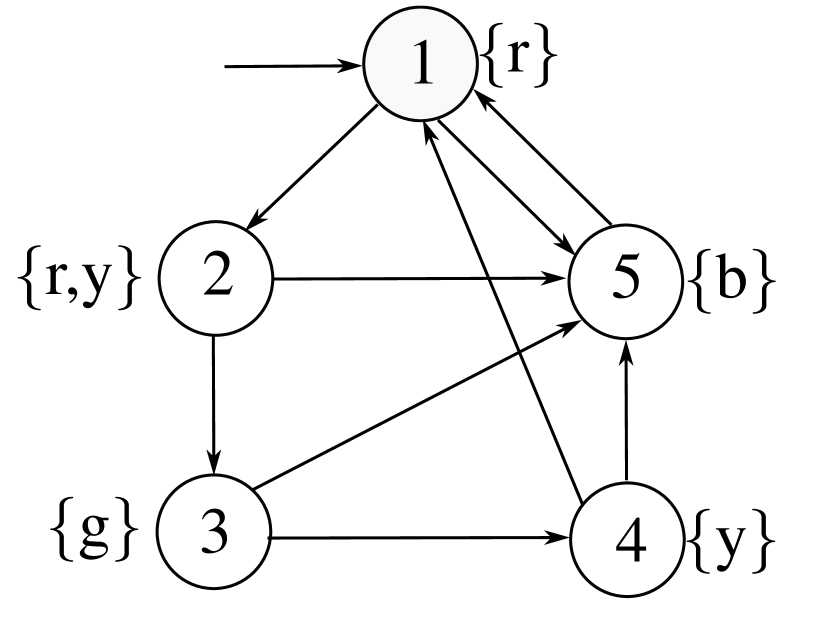
Example II.1.
A traffic light can be red, green, yellow or black (not working). The traffic light might stop working at any time. After it has been repaired, it turns red. Initially, the light is red. An illustration of such a traffic light is shown in Fig. 1(a). We can model the traffic light as a transition system :
-
•
;
-
•
;
-
•
;
-
•
;
-
•
. ∎
Remark II.1.
We can rewrite the following discrete-time autonomous system as an infinite transition system:
where , , , , and . Here, denotes the set of observations. At each time instant , the disturbance belongs to a compact set . Denote by the set of initial states. If is finite, the system can be rewritten as an infinite transition system with
-
•
;
-
•
, if and only if there exists such that ;
-
•
;
-
•
;
-
•
.∎
II-B Reachability Analysis
This subsection specifies the reachability analysis for a transition system . We first define the minimal reachable set and the maximal reachable set.
Definition II.6.
Consider a transition system and two sets . The -step minimal reachable set from to is defined as
The minimal reachable set from to is defined as
Lemma II.1.
For two sets , define
Then, .
Proof.
Definition II.7.
Consider a transition system and two sets . The -step maximal reachable set from to is defined as
The maximal reachable set from to is defined as
Lemma II.2.
For two sets , define
Then, .
Proof.
Similar to the proof of Lemma II.1. ∎
We define the robust invariant set and the invariant set in the following.
Definition II.8.
A set is said to be a robust invariant set of a transition system if for any , .
Definition II.9.
For a set , a set is said to be the largest robust invariant set in if each robust invariant set satisfies .
Lemma II.3.
For a set , define
Then, .
Proof.
It follows again from the Knaster-Tarski Theorem [42] that exists and it is a fixed point to the monotone function . Thus, we have that . ∎
Definition II.10.
A set is said to be an invariant set of a transition system if for any , .
Definition II.11.
For a set , a set is said to be the largest invariant set in if each invariant set satisfies .
Lemma II.4.
For a set , define
Then, .
Proof.
Similar to the proof of Lemma II.3. ∎
We can understand the reachable sets and invariant sets defined above as maps , , , and , respectively. In the following, we will refer to them as “reachability operators”.
II-C LTL
An LTL formula is defined over a finite set of atomic propositions and both logic and temporal operators. The syntax of LTL can be described as:
where and denote the “next” and “until” operators, respectively. By using the negation and conjunction operators, we can define disjunction: . By employing the until operator, we can define: (1) eventually, ; (2) always, ; and (3) weak-until, .
Definition II.12.
(LTL semantics) For an LTL formula and a trajectory , the satisfaction relation is defined as
Definition II.13.
Consider a transition system and an LTL formula . The semantics of the universal form of , denoted by , is
The semantics of the existential form of , denoted by , is
III Temporal Logic Trees
This section will introduce the notion of TLT and establish a satisfaction relation between a trajectory and a TLT. Then, we construct TLTs from LTL formulae and discuss the approximation relation between them.
III-A Definitions
Definition III.1.
A TLT is a tree for which the next holds:
-
•
each node is either a set node, a subset of , or an operator node, from ;
-
•
the root node and the leaf nodes are set nodes;
-
•
if a set node is not a leaf node, its unique child is an operator node;
-
•
the children of any operator node are set nodes.
Next we define the complete path and the minimal Boolean fragment for a TLT. Minimal Boolean fragments play an important role when simplifying the TLT for model checking and control synthesis in the following.
Definition III.2.
A complete path of a TLT is a sequence of nodes and edges from the root node to a leaf node. Any subsequence of a complete path is called a fragment of the complete path.
Definition III.3.
A minimal Boolean fragment of a complete path is one of the following fragments:
-
(i)
a fragment from the root node to the first Boolean operator node ( or ) in the complete path;
-
(ii)
a segment from one Boolean operator node to the next Boolean operator node in the complete path;
-
(iii)
a fragment from the last Boolean operator node of the complete path to the leaf node;
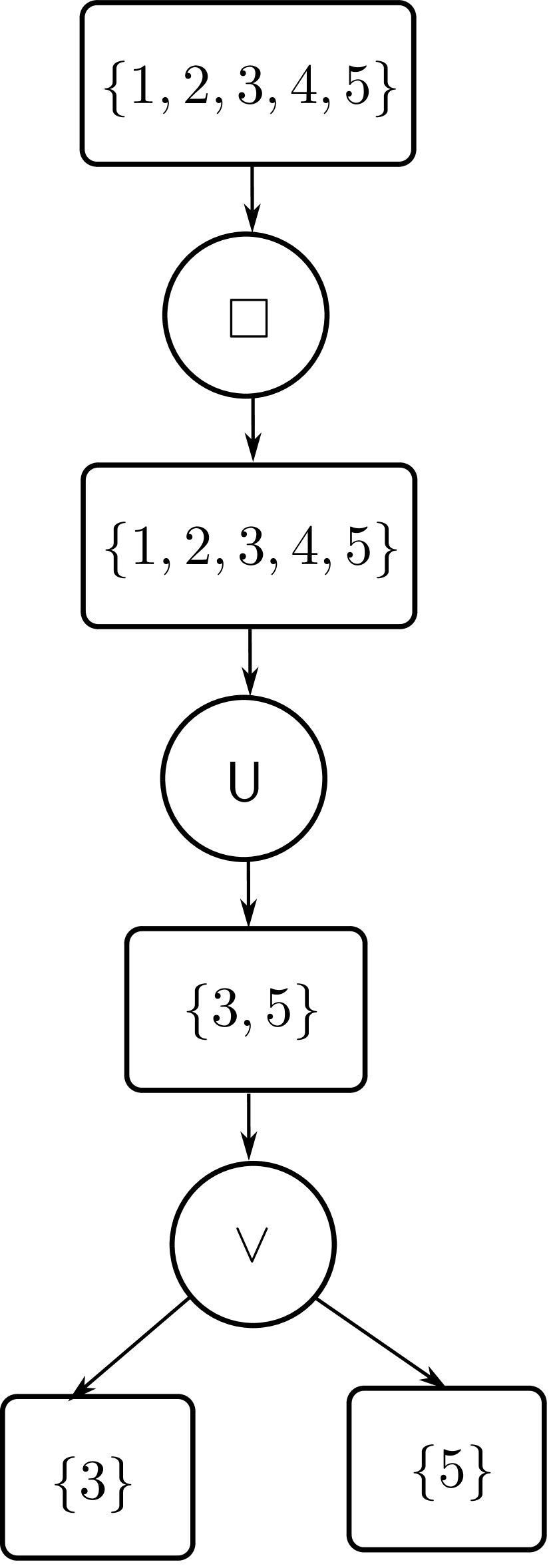
Example III.1.
Consider the traffic light in Example II.1 and the TLT in Fig. 1(b), which corresponds to the LTL formula (the formal construction of a TLT from an LTL formula will be detailed in next subsection). We encode one of the complete paths of this TLT in the form of , where , , and . For this complete path, the minimal Boolean fragments consist of and , which correspond to cases (i) and (iii) in Definition III.3, respectively. ∎
We now define the satisfaction relation between a given trajectory and a complete path of a TLT.
Definition III.4.
Consider a trajectory and encode a complete path of a TLT in the form of where is the number of operators in the complete path, for all and for all . The trajectory is said to satisfy this complete path if and there exists a sequence of time steps with for all and such that for all ,
-
(i)
if or , and ;
-
(ii)
if , and ;
-
(iii)
if , , , and ;
-
(iv)
if , , .
Consider a -th prefix from and a fragment from the complete path in the form of where . The prefix is said to satisfy this fragment if , , and there exists a sequence of time steps with for all and , such that for all , (i)–(iii) holds and furthermore
-
(iv’)
if , , .
Definition III.5.
A time coding of a TLT is an assignment of each operator node in the tree to a nonnegative integer.
Definition III.6.
Consider a trajectory and a TLT. The trajectory is said to satisfy the TLT if there exists a time coding such that the output of Algorithm 1 is .
The time coding indicates when the operators in the TLT are activated along a given trajectory. Algorithm 1 provides a procedure to test if a trajectory satisfies a TLT under a given time coding. The TLT is first transformed into a compressed tree, which is analogous to a binary decision diagram (lines 1–2), through Algorithm 2. Then, we check if the trajectory satisfies each complete path of the TLT under the time coding (lines 3–9). Finally, we backtrack the tree with output or . If the output is , the trajectory satisfies the TLT; otherwise, the trajectory does not satisfy the TLT under the given time coding.
Algorithm 2 aims to obtain a tree in a compact form. Each minimal Boolean fragment is encoded according to Definition III.3. The notation denotes the operator node and denotes the number of set nodes in the corresponding minimal Boolean fragment. We compress the sets in the minimal Boolean fragment to be a single set. The simplified tree consists of set nodes and Boolean operator nodes.
Example III.2.
Input: a trajectory , a TLT and a time coding
Output: or false;
Input: a tree
Output: a compressed tree
III-B Construction and Approximation of TLT
We define the approximation relations between TLTs and LTL formulae as follows.
Definition III.7.
A TLT is said to be an under-approximation of an LTL formula if all the trajectories that satisfy the TLT also satisfy .
Definition III.8.
A TLT is said to be an over-approximation of an LTL formula , if all the trajectories that satisfy also satisfy the TLT.
The following two theorems show how to construct TLTs via reachability analysis for the LTL formulae, and discuss their approximation relations.
Theorem III.1.
For any transition system and any LTL formula ,
-
(i)
a TLT can be constructed from the formula through the reachability operators and ;
-
(ii)
this TLT is an under-approximation of .
Proof.
Here we provide a proof sketch. See Appendix A for a detailed proof.
We prove the constructability by the following three steps: (1) we transform the given LTL formula into an equivalent LTL formula in the weak-until positive normal form; (2) for each atomic proposition , we show that a TLT can be constructed from (or ); (3) we leverage induction to show the following: given LTL formulae , , and in weak-until positive normal form, if TLTs can be constructed from , , and , respectively, then TLTs can also be constructed through reachability operators and from the formulae , , , , and , respectively.
We follow a similar approach to prove an under-approximation relation between the constructed TLT and the LTL formula. The under-approximation occurs due to the conjunction operator and the presence of branching in the transition system. ∎
Similarly, the following results hold.
Theorem III.2.
For any transition system and any LTL formula ,
-
(i)
a TLT can be constructed from the formula through the reachability operators and ;
-
(ii)
this TLT is an over-approximation of .
Proof.
The proof of the first part is similar to that of Theorem III.1 by replacing the universal quantifier and the reachability operators and with the existential quantifier and the operators and , respectively. Also, the proof of the second part is similar to that of Theorem III.1 by following the definition of the maximal reachability analysis. ∎
We call the constructed TLT of the universal TLT of and the TLT of the existential TLT of . We remark that the constructed TLT is not unique: this is because an LTL formula can have different equivalent expressions (e.g, normal forms). Despite this, the approximation relations between an LTL formula and the corresponding TLT still hold.
The following corollary shows that the approximation relation between TLTs and LTL formulae are tight for deterministic transition systems.
Corollary III.1.
For any deterministic transition system and any LTL formula , the universal TLT and the existential TLT of are identical.
Proof.
Remark III.1.
Computation of reachable sets plays a central role in the construction of the TLT. The computation of reachable sets is not the focus of this paper. Interested readers are referred to relevant results [38, 39, 40] and associated computational tools, e.g., the multi-parametric toolbox [43] and the Hamilton-Jacobi toolbox [44]. ∎
Example III.3.
Consider the traffic light in Example II.1 and the LTL formula in Example III.2 again. We follow the proof of Theorem III.1 to show the correspondence between and the TLT in Fig. 1(b):
-
(1)
the universal TLT of is a single set node, i.e., and the universal TLT of is also a single set node, i.e,, ;
-
(2)
the root node of the universal TLT of is the union of and , i.e., ;
-
(3)
the root node of the universal TLT of is ;
-
(4)
the root node of the universal TLT of is .
IV Model Checking via TLT
This section focuses on the model checking problem.
Problem IV.1.
Consider a transition system and an LTL formula . Verify whether , i.e., , .
Thanks to the approximation relations between the TLTs and the LTL formulae, we obtain the following lemma.
Lemma IV.1.
For any transition system and any LTL formula ,
-
(i)
if belongs to the root node of the universal TLT of ;
-
(ii)
only if belongs to the root node of the existential TLT of .
Proof.
The first result follows from that the root node of the universal TLT is an under-approximation of the satisfaction set of , as shown in Theorem III.1. Dually, the second result follows from that the root node of the universal TLT is an over-approximation of the satisfaction set of , shown in Theorem III.2. ∎
The next theorem provides two sufficient conditions for solving Problem IV.1.
Theorem IV.1.
For a transition system and an LTL formula , if one of the following conditions holds:
-
(i)
the initial state set is a subset of the root node of the universal TLT for ;
-
(ii)
no initial state from belongs to the root node of the existential TLT for .
Proof.
Similarly, we derive two necessary conditions for solving the model checking problem.
Theorem IV.2.
For a transition system and an LTL formula , only if one of the following conditions holds:
-
(i)
the initial state set is a subset of the root node of the existential TLT for ;
-
(ii)
no initial state from belongs to the root node of the universal TLT for .
Proof.
Similar to Theorem IV.1. ∎
Notice that the approximation relations between the TLT and the LTL formula are tight for deterministic transition systems, as shown in Corollary III.1. In this case, the model checking problem can be tackled as follows.
Corollary IV.1.
For a deterministic transition system and an LTL formula , if and only if the initial state set is a subset of the root node of the universal (or existential) TLT for .
Proof.
Follows from Corollary III.1. ∎
The conditions in Theorems IV.1–IV.2 imply that one can directly do model checking by using TLTs, as shown in the following example.
Example IV.1.
Let us continue to consider the traffic light and the LTL formula . Let us verify whether by using the above method. Since the unique initial state belongs to the root node of the universal TLT of shown in Fig. 1(b), it follows from condition (i) in Theorem IV.1 that . Next, we show how to use condition (ii) to verify that .
First of all, we have . Following the proof of Theorem III.2, we construct the existential TLT of :
-
(1)
the existential TLT of is a single set node, i.e., and the existential TLT of is also a single set node, i.e,, ;
-
(2)
the root node of the existential TLT of is the intersection of and , i.e., ;
-
(3)
the root node of the existential TLT of is .
As the existential TLT of is the empty set , this implies that condition (ii) in Theorem IV.1 holds and thus . ∎
V Control Synthesis via TLT
This section will show how to use the TLT to do control synthesis. Before that, we will introduce the notion of controlled transition system and recall the controlled reachability analysis.
V-A Controlled Transition System
Definition V.1.
A controlled transition system is a tuple consisting of
-
•
a set of states;
-
•
a set of control inputs;
-
•
a transition relation ;
-
•
a set of initial states;
-
•
a set of atomic propositions;
-
•
a labelling function .
Definition V.2.
A controlled transition system is said to be finite if , , and .
Definition V.3.
For and , the set of direct successors of under is defined by .
Definition V.4.
For , the set of admissible control inputs at state is defined by .
Definition V.5.
(Policy) For a controlled transition system , a policy is a sequence of maps . Denote by the set of all policies.
Definition V.6.
(Trajectory) For a controlled transition system , an infinite trajectory starting from under a policy is a sequence of states such that , . Denote by the set of infinite trajectories starting from under .
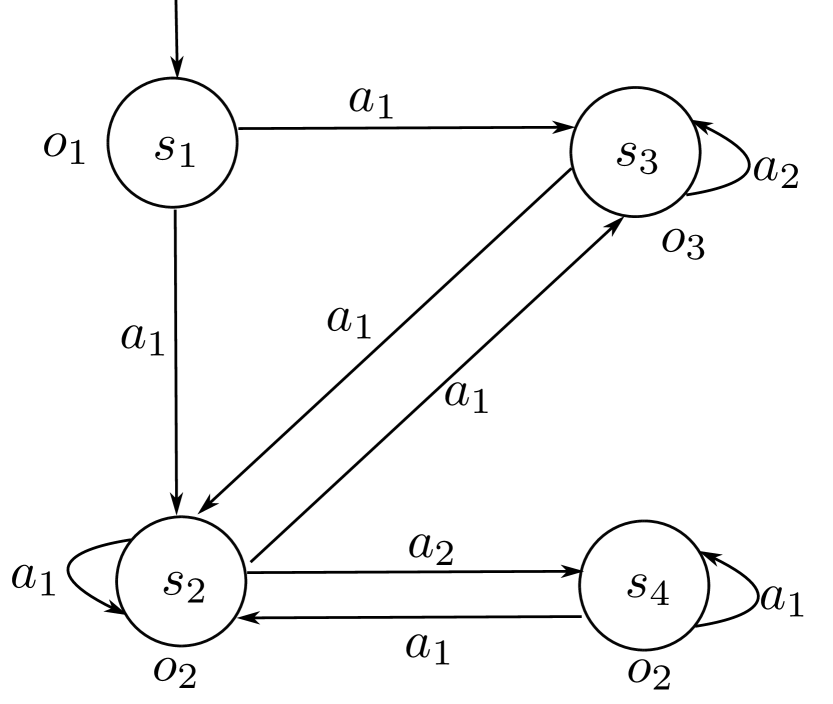
Example V.1.
A controlled transition system is shown in Fig. 2(a), where
-
•
;
-
•
;
-
•
;
-
•
;
-
•
;
-
•
. ∎
Remark V.1.
We express the following discrete-time uncertain control system as an infinite controlled transition system:
| (1) |
where and , , , , and . Here, denotes the set of observations. At each time instant , the control input is constrained by a compact set and the disturbance belongs to a compact set . Denote by the set of the initial states. If the observation set is finite, can be rewritten as an infinite controlled transition system, where
-
•
;
-
•
;
-
•
and , if and only if there exists such that ;
-
•
;
-
•
;
-
•
. ∎
V-B Controlled Reachability Analysis
This subsection will develop reachability analysis of a controlled transition system .
Definition V.7.
Consider a controlled transition system and two sets . The -step controlled reachable set from to is defined as
The controlled reachable set from to is defined as
Lemma V.1.
For two sets , define
Then, .
Proof.
Similar to the proof of Lemma II.1. ∎
Definition V.8.
A set is said to be a robust controlled invariant set (RCIS) of a transition system if for any , there exists such that .
Definition V.9.
For a set , a set is said to be the largest RCIS in if each RCIS satisfies .
Lemma V.2.
For a set , define
Then, .
Proof.
Similar to the proof of Lemma II.3. ∎
The definitions of controlled reachable sets and RCISs provide us a way to synthesize the feasible control set, which is detailed in Algorithm 4. In the following, we treat the maps and as the reachability operators.
V-C Construction and Approximation of TLT
The next theorem shows how to construct a TLT from an LTL formula for a controlled transition system and discusses its approximation relation.
Theorem V.1.
For a controlled transition system and any LTL formula , the following holds:
-
(i)
a TLT can be constructed from the formula through the reachability operators and ;
-
(ii)
given an initial state , if there exists a policy such that satisfies the constructed TLT, , then , .
Proof.
The proof of the first part is similar to that of Theorem III.1 by replacing the reachability operators and with and , respectively.
Similar to the under-approximation of the universal TLT in Theorem III.1, we can show that the path satisfying the constructed TLT in the first part also satisfies the LTL formula. Then, we can directly prove the second result. ∎
Let us call the constructed TLT of in Theorem V.1 the controlled TLT of .
Remark V.2.
Checking whether there exists a policy, such that all the resulting trajectories satisfy the obtained controlled TLT, is in general a hard problem. A straightforward necessary condition is that belongs to the root node of the controlled TLT: however, this is neither a necessary nor a sufficient condition on the existence of a policy such that all the resulting trajectories satisfy the given LTL formula. A (rather conservative) necessary condition for the latter case can be obtained by regarding the controlled TS as a non-deterministic transition system, and then applying Thereom IV.2. ∎
Next we will show how to construct the controlled TLT through an example.
V-D Control Synthesis Algorithm
In this subsection, we solve the following control synthesis problem.
Problem V.1.
Consider a controlled transition system and an LTL formula . For an initial state , find, whenever existing, a sequence of feedback control inputs such that the resulting trajectory satisfies .
Remark V.3.
Note that the objective of the above problem is not to find a policy , but a sequence of control inputs that depend on the measured state. In general, synthesizing a policy such that each trajectory satisfies is computationally intractable for infinite systems. Instead, here we seek to find online a feasible control input at each time step, in a similar spirit to constrained control or receding horizon control. ∎
Instead of directly solving Problem V.1, we consider the following related task, whose solution is also a solution to Problem V.1, thanks to Theorem V.1.
Problem V.2.
Consider a controlled transition system and an LTL formula . For an initial state , find, whenever existing, a sequence of control inputs such that the resulting trajectory satisfies the controlled TLT constructed from .
Algorithm 3 provides a solution to Problem V.2. In particular, Algorithm 3 presents an online feedback control synthesis procedure, which consists of three steps: (1) control tree: replace each set node of the TLT with a corresponding control set candidate (Algorithm 4); (2) compressed control tree: compress the control tree as a new tree whose set nodes are control sets and whose operator nodes are conjunctions and disjunctions (Algorithm 2); (3) backtrack on the control sets through a bottom-up traversal over the compressed control tree (Algorithm 5). If the output of Algorithm 5 is , there does not exist a feasible solution to Problem V.2. We remark that Algorithm 3 is implemented in a similar way to receding horizon control with the prediction horizon being one.
Input: an initial state and the controlled TLT of an LTL formula
Output: or with and
Input: and a TLT
Output: a control tree
Algorithm 4 aims to construct a control tree that enjoys the same tree structure as the input TLT. The difference is that all the set nodes are replaced with the corresponding control set nodes. The correspondence is established as follows: (1) whether the initial state belongs to the root node or not (lines 1–3); (2) whether the prefix satisfy the fragment from the root node to the set node (lines 5–7); (4) whether or not the set node is a leaf node (lines 9–14); (5) which operator the child of the set node is (lines 16–24).
Algorithm 5 aims to backtrack a set by using the compressed tree. We update the parent of each Boolean operator node through a bottom-up traversal.
Input: a compressed tree
Output: a set
Note that the construction of a control tree in Algorithm 4 is closely related to the controlled reachability analysis in Section V-B. In lines 12–13, the computation of control set follows from the definition of RCIS. In lines 22–23, the definition of one-step controlled reachable set is used to compute the control set. In lines 24–26, the control set is synthesized from the definition of a controlled reachable set.
The following theorem shows that Algorithm 3 is recursively feasible. This means that initial feasibility implies future feasibility. This is an important property, particularly used in receding horizon control.
Theorem V.2.
Consider a controlled transition system , an LTL formula , and an initial state . Let and the controlled TLT of be the inputs of Algorithm 3. If there exists a policy such that satisfies the controlled TLT of , , then
-
(i)
the control set (line 8 of Algorithm 3) is nonempty for all ;
-
(ii)
at each time step , there exists at least one trajectory with prefix under some policy such that satisfies the controlled TLT of , and .
Proof.
The proof follows from the construction of the set in Algorithm 4 and the operations in Algorithms 2 and 5, and the definitions of controlled reachable sets and RCIS. If there exists a policy such that satisfies the controlled TLT of , , we have that Algorithm 3 is feasible at each time step , which implies that . Furthermore, from Algorithm 4, each element in guarantees the one-step ahead feasibility for all realizations of , which implies the result (ii). ∎
Theorem V.2 implies that if there exists a policy such that all the resulting trajectories satisfy the controlled TLT built from , then Algorithm 3 is always feasible at each time step in two senses: (1) the control set is nonempty; and (2) there always exists a feasible policy such that the trajectories with the realized prefix satisfy the controlled TLT.
Remark V.4.
In Algorithm 3, the integration of Algorithms 2, 4, and 5 can be interpreted as a feedback control law. This control law is a set-valued map at time step . Given the prefix , this map collects all the feasible control inputs such that the state can move along the TLT from . ∎
Remark V.5.
Note that to implement Algorithm 3, we do not need to first check for the existence of a policy for the controlled TLT. The fact that a non-empty control set is synthesized by Algorithm 3 at each time step is necessary for the existence of the policy for the controlled TLT. We use the existence of the policy as a-priori condition for proving the recursive feasibility of Algorithm 3 in Theorem V.1. ∎
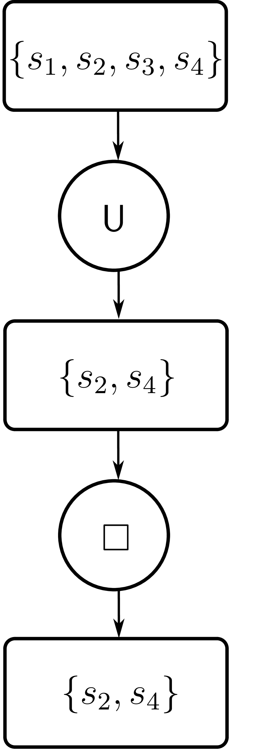
Example V.3.
Let us continue to consider the controlled transition system in Example V.1 and the LTL formula in Example V.2. Implementing Algorithm 3, we obtain Table I. We can see that at each time step, we can synthesize a nonempty feedback control set. One realization is , of which the trajectory satisfies both the controlled TLT and the formula .
In this example, Algorithm 3 is recursively feasible since we can verify that the condition in Theorem V.2 holds. That is, there exists a policy such that all the resulting trajectories satisfy the controlled TLT: a feasible stationary policy is , where with , and . Under this policy, there are two possible trajectories, and , both of which satisfy the controlled TLT and the LTL formula . ∎
| Time | State | Control set | Control input |
|---|---|---|---|
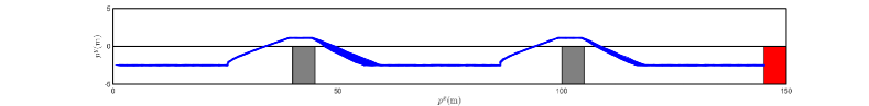
VI Examples
VI-A Obstacle Avoidance
Following the example of obstacle avoidance for double integrator in [45], we consider the following dynamical system
| (6) |
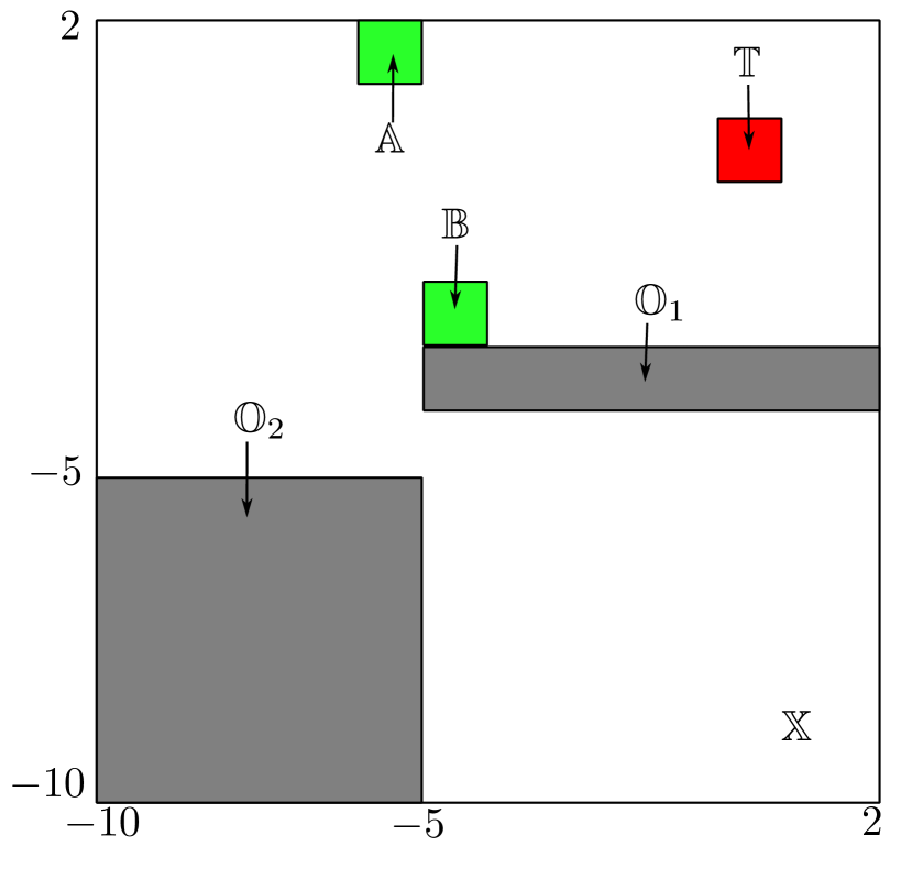
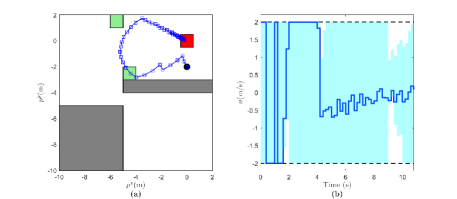
Different from [45], we choose the smaller sampling time of second and take into account the disturbance . We consider the same scenario as in [45], as shown in Fig. 3(a). The working space is , the control constraint set is , and the disturbance set is . In Fig. 3(a), the obstacle regions are and , the target region is , and two visiting regions are and .
Recall the system (1). Let the set of the observations be and, if , we define the observation function as
| (7) |
As shown in Remark V.1, we can rewrite the system (6) with the observation function (7) as a controlled transition system with the set of atomic propositions and the labelling function .
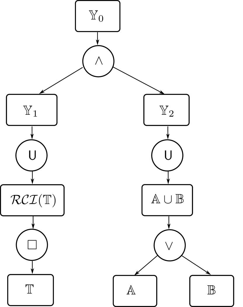
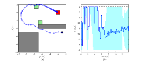
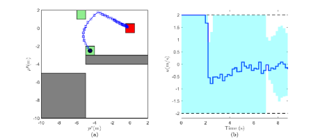
In [45], the specification is to visit the region or region , and then the target region , while always avoiding obstacles and , and staying inside the working space . This specification can be expressed as a co-safe LTL formula . Here, we extend the specification to be to visit region or region , and then visit and always stay inside the target region , while always avoiding obstacles and , and staying inside working space . Obviously, this specification cannot be expressed as a co-safe LTL formula, and thus cannot be handled by the approach in [45]. We instead express this specification as the LTL formula . We will show that our approach can handle such non-co-safe LTL formula. By computing inner approximations of the controlled reachable sets, we can construct the controlled TLT of and then use Algorithm 3 to synthesize controllers online. The constructed controlled TLT for is shown in Fig. 3(b). Similar to [45], we choose three different initial states, for each of which the state trajectories and the control trajectories are shown in Figs. 4–6. We can see that in Figs. 4–6 (a), all state trajectories satisfy the required specification . The black dots are the initial state. In this example, the target region is a RCIS. After entering , the states stay there by using the controllers that ensure robust invariance. In Figs. 4–6 (b), the dashed lines denote the control bounds, the cyan regions represent the synthesized control sets in Algorithm 3, and the blue lines are the implemented control inputs.
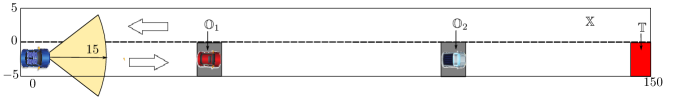
VI-B Online Specification Update
This example will show how the specification can be updated online when using our approach. As shown in Fig. 7, we consider a scenario where an automated vehicle plans to move to a target set but with some unknown obstacles on the road. The sensing region of the vehicle is limited. We use a single integrator model with a sample period of second to model the dynamics of the vehicle:
| (12) |
The working space is , the control constraint set is , the disturbance set is , and the target region is . We assume that , , and are known a priori to the vehicle and the vehicle should move along the lane with the right direction unless lane change is necessary. In Fig. 7, there are two broken vehicles in the sets and . We assume that and are unknown to the vehicle at the beginning. As long as the vehicle can sense them, they are known to the vehicle.
Let the initial state be and the sensing limitation is . At time step , the set of observations is and if , we define the observation function as
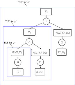
The initial specification can be expressed as an LTL . By constructing the controlled TLT of shown in Fig. 8 and implementing Algorithm 3, we obtain one realization as shown in Fig. 9. We can see that the vehicle keeps moving straightforward until it senses the obstacle at .
When the vehicle can sense , a new observation with and is added to the set , which becomes . If , we update the observation function as
To avoid , the new specification is changed to be . We can construct the TLT of based on that of , which is shown in Fig. 8, and then continue to implement Algorithm 3. We can see that the vehicle changes lane from and quickly merges back after overtaking . The trajectories are shown in Fig. 9. The vehicle is under the control with respect to until it can sense at .
Similarly, when the vehicle can sense , we update and the observation function as if ,
To avoid , the new specification is changed to be . We can construct the TLT of based on that of , which is shown in Fig. 8, and then continue to implement Algorithm 3. We can see that the vehicle changes lane from and quickly merges back after overtaking . Under the control with respect to , the vehicle finally reaches the target set .
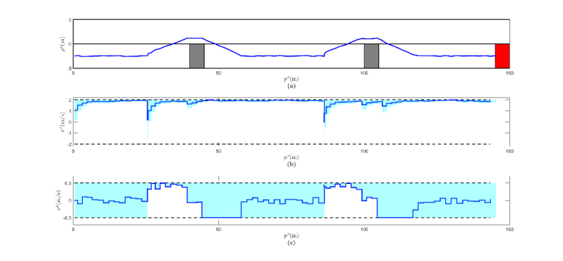
Fig. 9 (a) shows the state trajectories, from which we can see that the whole specification is completed. Fig. 9 (b)–(c) show the corresponding control inputs, where the dashed lines denote the control bounds. The cyan regions represent the synthesized control sets and the blue lines are the control trajectories. Furthermore, we repeat the above process for 100 realizations of the disturbance trajectories. The state trajectories for such 100 realizations are shown in Fig. 10.
We remark that in this example, the control inputs are chosen to push the state to move down along the TLT as fast as possible. In detail, if the state is the -step reachable set in the set node , we can generate a smaller control set from which the control input can push the state to the -step reachable set. That is what we can see from Fig. 9, where almost all control inputs in the synthesized control sets along -axis are positive.
VII Conclusions and Future Work
We have studied LTL model checking and control synthesis for discrete-time uncertain systems. Quite unlike automaton-based methods, our solutions build on the connection between LTL formulae and TLT structures via reachability analysis. For a transition system and an LTL formula, we have proved that the TLTs provide an underapproximation or overapproximation for the LTL via minimal and maximal reachability analysis, respectively. We have provided sufficient conditions and necessary conditions to the model checking problem. For a controlled transition system and an LTL formula, we have shown that the TLT is an underapproximation for the LTL formula and thereby proposed an online control synthesis algorithm, under which a set of feasible control inputs is generated at each time step. We have proved that this algorithm is recursively feasible. We have also illustrated the effectiveness of the proposed methods through several examples.
Future work includes the extension of TLTs to handle other general specifications (e.g., CTL∗) and a broad experimental evaluation of our approach.
Acknowledgements
The authors are grateful to Dr. Xiaoqiang Ren (Shanghai University) and Mr. Hosein Hasanbeig (University of Oxford) for helpful discussions and feedback.
Appendix A. Proof of Theorem III.1
The whole proof is divided into two parts: the first part shows how to construct a TLT from the formula by means of the reachability operators and , while the second part shows that such TLT is an underapproximation for .
Construction: We follow three steps to construct a TLT.
Step 1: rewrite the given LTL in the weak-until positive normal form. From [4], each LTL formula has an equivalent LTL formula in the weak-until positive normal form, which can be inductively defined as
| (13) |
Step 2: for each atomic proposition , construct the TLT with only a single set node from or . In detail, the set node for is while the set node for is . In addition, the TLT for (or ) also has a single set node, which is (or ).
Step 3: based on Step 2, follow the induction rule to construct the TLT for any LTL formula in the weak-until positive normal form. More specifically, we will show that given the LTL formulae , , and in the weak-until positive normal form, if the TLTs can be constructed from , , and , respectively, then the TLTs can be thereby constructed from the formulae , , , , and , respectively.
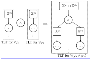
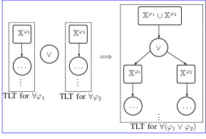
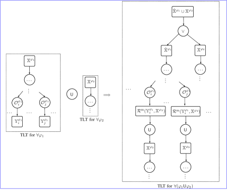
For (or ), we construct the TLT by connecting the root nodes of the TLTs for and through the operator (or ) and taking the intersection (or union) of two root nodes, as shown in Fig. 11(a)–(b). For , we denote by the root node of the TLT for and then construct the TLT by adding a new set node to be the parent of and connecting them through the operator , as shown in Fig. 11(c).
For , the TLT construction is as follows. Denote by all the pairs comprising a leaf node and its corresponding parent in the TLT of , where is the number of the leaf nodes. Here, is the th leaf node and is its parent. Denote by the root node of TLT for . We first change each leaf node to . We then update the new tree for from the leaf node to the root node according to the definition of the operators. After that, we take copies of the TLT of . We set the root node of each copy as the child of each new leaf node, respectively, and connect them trough the operator . Finally, we have one more copy of the TLT of and connect this copy and the new tree trough the disjunction . An illustrative diagram is given in Fig. 11(d).
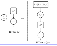
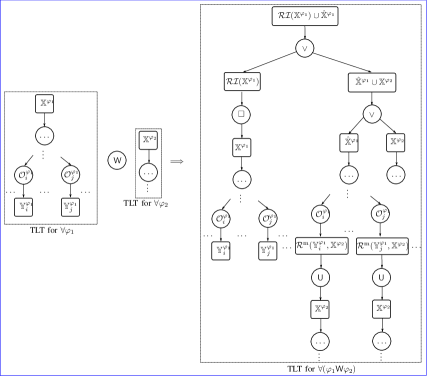
For the fragment , we first recall that . Let and . Denote by the root node of the TLT for . We first construct the TLT of as described above. Second, we further construct the TLT of with by adding a new node as the parent of and connecting them through . Then, we construct the TLT of . An illustrative diagram is given in Fig. 11(e).
Underapproximation: First, it is very easy to verify that the constructed TLT above with a single set node (or or ) for (or or or ) is an underapproximation for (or or or ) and the underapproximation relation in these cases is also tight.
Next we also follow the induction rule to show that the constructed TLT from is an underapproximation for . Consider LTL formulae , , and . We will show that if the constructed TLTs of , , and are the underapproximations of , , and , respectively, then the TLTs constructed above for the formulae , , , , and are the underapproximations of , , , , and , respectively.
According to the set operation (intersection or union) or the definition of one-step minimal reachable set, it is easy to verify that the constructed TLT for (or ) or is an underapproximation for (or ) or if the TLTs of and , and are underapproximations , , and , respectively.
Let us consider . Assume that a trajectory satisfies the TLT of . Recall the construction of the TLT of from and . According to the definition of minimal reachable set, we have (1) satisfies the TLT of ; or (2) there exists that such that satisfies the TLT of and for all , the trajectory satisfies the the TLT of . Under the assumption that the TLTs of and are the underapproximations of and , respectively, we have that there exists such that and for all , , which implies that . Thus, the TLT of is an approximation of .
Recall that . Following the proofs for until operator and the disjunction and the definition of the robust invariant set, it yields that the constructed TLT of is an underapproximation of .
The proof is complete. ∎
References
- [1] K. J. Åström and B. Wittenmark, Computer-controlled Systems: Theory and Design. Courier Corporation, 2013.
- [2] P. Tabuada, Verification and Control of Hybrid Systems: A Symbolic Approach. Springer, 2009.
- [3] R. Alur, Principles of Cyber-Physical Systems. MIT Press, 2015.
- [4] C. Baier and J.-P. Katoen, Principles of Model Checking. MIT press, 2008.
- [5] M. Y. Vardi, “An automata-theoretic approach to linear temporal logic,” in Logics for Concurrency, F. Moller and G. Birtwistle, Eds. Springer, 1996, pp. 238–266.
- [6] M. O. Rabin, “Decidability of second-order theories and automata on infinite trees,” Transactions of the American Mathematical Society, no. 141, pp. 1–35, 1969.
- [7] E. A. Emerson, “Automata, tableaux, and temporal logics,” in Proceedings of Workshop on Logic of Programs, 1985, pp. 79–88.
- [8] N. Piterman and A. Pnueli, “Faster solutions of rabin and streett games,” in Proceedings of 21st Annual IEEE Symposium on Logic in Computer Science, 2006, pp. 275–284.
- [9] F. Horn, “Streett games on finite graphs,” in Proceedings of 2nd Workshop on Games in Design and Verification, 2005.
- [10] A. Girard and G. J. Pappas, “Approximation metrics for discrete and continuous systems,” IEEE Transactions on Automatic Control, vol. 5, no. 52, pp. 782–798, 2007.
- [11] A. Girard, G. Pola, and G. J. Pappas, “Approximately bisimilar symbolic models for incrementally stable switched systems,” IEEE Transactions on Automatic Control, vol. 1, no. 55, pp. 116–126, 2010.
- [12] M. Zamani, P. M. Esfahani, R. Majumdar, A. Abate, and J. Lygeros, “Symbolic control of stochastic systems via approximately bisimilar finite abstractions,” IEEE Transactions on Automatic Control, vol. 12, no. 59, pp. 3135–3150, 2014.
- [13] M. Zamani, G. Pola, M. Mazo, and P. Tabuada, “Symbolic models for nonlinear control systems without stability assumptions,” IEEE Transactions on Automatic Control, vol. 7, no. 57, pp. 1804–1809, 2012.
- [14] P. Yu and D. V. Dimarogonas, “Approximately symbolic models for a class of continuous-time nonlinear systems,” in Proceedings of 58th IEEE Conference on Decision and Control, 2019, pp. 4349–4354.
- [15] P. Tabuada and G. J. Pappas, “Model checking LTL over controllable linear systems is decidable,” in Proceedings of ACM International Conference on Hybrid Systems: Computation and Control, 2003, pp. 498–513.
- [16] B. Yordanov, J. Tumová, I. Černá, J. Barnat, and C. Belta, “Formal analysis of piecewise affine systems through formula guided refinement,” Automatica, vol. 1, no. 49, pp. 261–266, 2013.
- [17] ——, “Temporal logic control of discrete-time piecewise affine systems,” IEEE Transactions on Automatic Control, vol. 6, no. 57, pp. 1491–1504, 2012.
- [18] P.-J. Meyer and D. V. Dimarogonas, “Hierarchical decomposition of LTL synthesis problem for nonlinear control systems,” IEEE Transactions on Automatic Control, vol. 11, no. 64, pp. 4676–4683, 2019.
- [19] S. Haesaert and S. Soudjani, “Robust dynamic programming for temporal logic control of stochastic systems,” 2018. [Online]. Available: arXiv:1811.11445
- [20] S. Karaman, R. G. Sanfelice, and E. Frazzoli, “Optimal control of mixed logical dynamical systems with linear temporal logic specifications,” in Proceedings of 47th IEEE Conference on Decision and Control, 2008, pp. 2117–2122.
- [21] N. Cauchi and A. Abate, “StocHy-automated verification and synthesis of stochastic processes,” in Proceedings of ACM International Conference on Hybrid Systems: Computation and Control, 2019, pp. 258–259.
- [22] A. Ulusoy and C. Belta, “Receding horizon temporal logic control in dynamic environments,” The International Journal of Robotics Research, vol. 12, no. 33, pp. 1593–1607, 2014.
- [23] M. Guo, J. Tumová, and D. V. Dimarogonas, “Communication-free multi-agent control under local temporal tasks and relative-distance constraints,” IEEE Transactions on Automatic Control, vol. 12, no. 61, pp. 3948–3962, 2016.
- [24] S. Coogan, E. A. Gol, M. Arcak, and C. Belta, “Traffic network control from temporal logic specifications,” IEEE Transactions on Control of Network Systems, vol. 2, no. 3, pp. 162–171, 2016.
- [25] X. Ding, M. Lazar, and C. Belta, “LTL receding horizon control for finite deterministic systems,” Automatica, vol. 2, no. 50, pp. 399–408, 2014.
- [26] T. Wongpiromsarn, U. Topcu, and R. M. Murray, “Receding horizon temporal logic planning,” IEEE Transactions on Automatic Control, vol. 11, no. 57, pp. 2817–2830, 2012.
- [27] P. Schillinger, M. Bürger, and D. V. Dimarogonas, “Hierarchical LTL-task MDPs for multi-agent coordination through auctioning and learning,” 2019. [Online]. Available: http://kth.diva-portal.org
- [28] L. Lindemann and D. V. Dimarogonas, “Feedback control strategies for multi-agent systems under a fragment of signal temporal logic tasks,” Automatica, vol. 106, pp. 284–293, 2019.
- [29] M. Kwiatkowska, G. Norman, and D. Parker, “PRISM 4.0: verification of probabilistic real-time systems,” in Proceedings of 23rd International Conference on Computer Aided Verification, 2011, pp. 585–591.
- [30] C. Belta, “Formal synthesis of control strategies for dynamical systems,” in Proceedings of 55th IEEE Conference on Decision and Control, 2016, pp. 3407–3431.
- [31] C. Belta, B. Yordanov, and E. A. Gol, Formal Methods for Discrete-time Dynamical Systems. Springer, 2017.
- [32] P. G. Sessa, D. Frick, T. A. Wood, and M. Kamgarpour, “From uncertainty data to robust policies for temporal logic planning,” in Proceedings of ACM International Conference on Hybrid Systems: Computation and Control, 2018, pp. 157–166.
- [33] K. Hashimoto and D. V. Dimarogonas, “Resource-aware networked control systems under temporal logic specifications,” Discrete Event Dynamic Systems, 2019.
- [34] M. Inoue and V. Gupta, “‘Weak’ control for human-in-the-loop systems,” IEEE Control Systems Letters, vol. 3, no. 2, pp. 440–445, 2018.
- [35] Y. Gao, F. J. Jiang, X. Ren, L. Xie, and K. H. Johansson, “Reachability-based human-in-the-loop control with uncertain specifications,” in Proceedings of 21st IFAC World Congress, 2020, to appear.
- [36] F. Blanchini and S. Miani, Set-theoretic Methods in Control. Springer, 2007.
- [37] J. Lygeros, C. Tomlin, and S. Sastry, “Controllers for reachability specifications for hybrid systems,” Automatica, vol. 3, no. 35, pp. 349–370, 1999.
- [38] M. Chen, S. L. Herbert, M. S. Vashishtha, S. Bansal, and C. J. Tomlin, “Decomposition of reachable sets and tubes for a class of nonlinear systems,” IEEE Transactions on Automatic Control, vol. 11, no. 63, pp. 3675–3688, 2018.
- [39] M. Althoff and B. H. Krogh, “Reachability analysis of nonlinear differential-algebraic systems,” IEEE Transactions on Automatic Control, vol. 2, no. 59, pp. 371–383, 2014.
- [40] I. M. Mitchell, “Scalable calculation of reach sets and tubes for nonlinear systems with terminal integrators: a mixed implicit explicit formulation,” in Proceedings of ACM International Conference on Hybrid Systems: Computation and Control, 2011, pp. 103–112.
- [41] M. Chen, Q. Tam, S. C. Livingston, and M. Pavone, “Signal temporal logic meets Hamilton-Jacobi reachability: connections and applications,” in Proceedings of International Workshop on the Algorithmic Foundations of Robotics, 2018. [Online]. Available: http://asl.stanford.edu/wp-content/papercite-data/pdf/Chen.Tam.Livingston.Pavone.WAFR18.pdf
- [42] A. Tarski, “A lattice-theoretical fixpoint theorem and its application,” Pacific Journal of Mathematics, no. 5, pp. 285–309, 1955.
- [43] M. Herceg, M. Kvasnica, C. N. Jones, and M. Morari, “Multi-parametric toolbox 3.0,” in Proceedings of European Control Conference, 2013, pp. 502–510.
- [44] I. M. Mitchell and J. A. Templeton, “A toolbox of Hamilton-Jacobi solvers for analysis of nondeterministic continuous and hybrid systems,” in Proceedings of ACM International Conference on Hybrid Systems: Computation and Control, 2005, pp. 480–494.
- [45] E. A. Gol, M. Lazar, and C. Belta, “Language-guided controller synthesis for linear systems,” IEEE Transactions on Automatic Control, vol. 5, no. 59, pp. 1163 – 1176, 2014.