ExoMol line lists – XXXIX. Ro-vibrational molecular line list for CO₂

Abstract

A new hot line list for the main isotopologue of CO₂, ¹²C¹⁶O₂ is presented. The line list consists of almost 2.5 billion transitions between 3.5 million rotation-vibration states of CO₂ in its ground electronic state, covering the wavenumber range 0–20 000 cm^-1 ($\lambda>0.5$ $\mu$m) with the upper and lower energy thresholds of 36 000 cm^-1 and 16 000 cm^-1, respectively. The ro-vibrational energies and wavefunctions are computed variationally using the Ames-2 accurate empirical potential energy surface. The ro-vibrational transition probabilities in the form of Einstein coefficients are computed using an accurate ab initio dipole moment surface using variational program TROVE. A new implementation of TROVE which uses an exact nuclear-motion kinetic energy operator is employed. Comparisons with the existing hot line lists are presented. The line list should be useful for atmospheric retrievals of exoplanets and cool stars. The UCL-4000 line list is available from the CDS and ExoMol databases.

1 Introduction

Carbon dioxide is well-known and much studied constituent of the Earth’s atmosphere. However, it is also an important constituent of planetary atmospheres. The Venusian atmosphere is 95% CO₂ which therefore dominates its opacity (Snels et al., 2014). Similarly studies of exoplanets have emphasised the importance of CO₂. It was one of the first molecules detected in the atmospheres of hot Jupiter exoplanets (Swain et al., 2009a, b, 2010) where it provides an important measure of the C/O ratio on the planet (Moses et al., 2013). Similarly it is considered an important marker in directly imaged exoplanets (Moses et al., 2013) and the atmospheres of lower mass planets are expected to be dominated by water and CO₂ (Massol et al., 2016). Heng & Lyons (2016) provide a comprehensive study of CO₂ abundances in exoplanets. Recently, Baylis-Aguirre et al. (2020) detected emission and absorption from excited vibrational bands of CO₂ in the mid-infrared spectra of the M-type Mira variable R Tri using the Spitzer infrared spectrograph (IRS).

Most of the environments discussed above are considerably hotter then the Earth: for example Venus is at about 735 K and hot Jupiter exoplanets have typical atmospheric temperatures in excess of 1000 K. Hot CO₂ is also important for industrial applications on Earth (Evseev et al., 2012) and studies of combustion engines (Rein & Sanders, 2010). These applications all require information on CO₂ spectra at higher temperatures. It is this problem that we address here.

The importance of CO₂ has led to very significant activity on the construction of list of important rotation-vibration transition lines. The HITRAN data base provides such lists for studies of the Earth’s atmosphere and other applications at or below 300 K. The CO₂ line lists where comprehensively updated in the 2016 release of HITRAN (Gordon & et al., 2017) in part to provide higher accuracy data to meet the demands of Earth observation satellites such as OCO-2 (Connor et al., 2016; Oyafuso et al., 2017). The 2016 update made extensive use of variational nuclear motion calculations (Zak et al., 2016, 2017b, 2017a) of the type employed here.

HITRAN is not designed for or suitable for high temperature applications which demand much more extensive line lists. The HITEMP data base (Rothman et al., 2010) is designed to address this issue. The original HITEMP used the direct numerical diagonalization calculations of Wattson & Rothman (1992), which were an early example of the use of large scale variational nuclear motion calculations to provide molecular line lists. The 2010 HITEMP update used the CDSD-1000 (carbon dioxide spectroscopic databank) line list (Tashkun et al., 2003). The CDSD-1000 line list is based on the use effective Hamiltonian fits to experimental data and was designed to be complete for temperatures up to 1000 K. CDSD-1000 subsequently was replaced by CDSD-4000. The empirical CO₂ line list CDSD-4000 computed by Tashkun & Perevalov (2011) is designed for temperatures up to 5000 K, but has limited wavenumber coverage. Furthermore, while usually good at reproducing known spectra, experience has shown that the effective Hamiltonian approach can struggle to capture all the unobserved hot bands resulting in underestimates of the opacity at higher temperatures (Chubb et al., 2020). A compact version of CDSD-4000 has recently been made available (Vargas et al., 2020).

The NASA Ames group have produced a number of CO₂ line lists (Huang et al., 2013, 2014, 2017, 2019) using highly accurate potential energy surfaces (Huang et al., 2012, 2017) and variational nuclear motion calculations. Most relevant for this work is the Ames-2016 CO₂ line list of Huang et al. (2017) which considers wavenumbers up to 15 000 cm^-1 and $J$ up to 150 with upper state energies limited to $hc\times$24 000 cm^-1. Due to this fixed upper energy cut-off, the temperature coverage depends on the wavenumber range, from $T\sim 4000$ K at lower end up to $\sim 1500$ K at the higher end. The Ames-2016 line list was based on an accurate empirically-generated potential energy (PES) surface Ames-2 and their high-level ab initio dipole moment surface (DMS) DMS-N2.

High accuracy room temperature line lists for 13 isotopologues of CO₂ was computed by Zak et al. (2016, 2017b, 2017a), using the Ames-2 PES (Huang et al., 2017) and UCL’s highly accurate DMS (Polyansky et al., 2015). These line lists are now part of the HITRAN (Gordon & et al., 2017) and ExoMol (Tennyson & Yurchenko, 2012) databases. The room temperature properties of this line list have been subject to a number experimental tests and the results have been found to be competitive in accuracy to state-of-the-art laboratory experiments (Odintsova et al., 2017; Kang et al., 2018; Čermák et al., 2018; Long et al., 2020).

Here we present a new hot line list for the main isotopologue of CO₂ (¹²C¹⁶O₂) generated using UCL’s ab initio DMS (Polyansky et al., 2015) and the empirical PES Ames-2 (Huang et al., 2017) with the variational program TROVE (Yurchenko et al., 2007). Our line list is the most comprehensive (complete and accurate) data set for CO₂. This work is performed as part of the ExoMol project (Tennyson & Yurchenko, 2012) and the results form an important addition to the ExoMol database (Tennyson et al., 2016) which, as discussed below, is currently being upgraded (Tennyson et al., 2020).

2 TROVE specifications

For this work we used a new implementation of the exact kinetic energy (EKE) operator for triatomics in TROVE (Yurchenko & Mellor, 2020) based on the bisector embedding for triatomic molecules (Carter et al., 1983; Sutcliffe & Tennyson, 1991).

The variational TROVE program (Yurchenko et al., 2007) solves the ro-vibrational Schrödinger equation using a multi-layer contraction scheme (see, for example, Yurchenko et al. (2017)). At step 1, the 1D primitive basis set functions $\phi_{v_{1}}(r_{1})$, $\phi_{v_{2}}(r_{2})$ (stretching) and $\phi_{v_{3}}(\rho)$ (bending) are obtained by numerically solving the corresponding Schrödinger equations. Here $r_{1}$ and $r_{2}$ are two stretching valence coordinates and $\rho=180^{\circ}-\alpha$ with $\alpha$ being the inter-bond valence angle. A 1D Hamiltonian operator for a given mode is constructed by setting all other degrees of freedom to the their equilibrium values. The two equivalent stretching equations are solved on a grid of 1000 points using the Numerov-Cooley approach (Noumerov, 1924; Cooley, 1961), with the grid values of $r_{i}$ ranging from $r_{\rm e}-0.4$ to $r_{\rm e}+1.0$ Å. The bending mode solutions are obtained on the basis of the associated Laguerre polynomials as given by

$$\phi_{n,l}^{(l)}(\rho)=C_{n,l}\,\rho^{l+1/2}\,L_{n}^{(l)}(a\rho^{2})\,e^{-a\rho^{2}/2},$$ (1)

normalized as

$$\int_{0}^{\rho_{\rm max}}\phi_{n,l}^{(l)}(\rho)^{2}\,d\rho=1,$$

where $a$ is a structural parameter, $l\geq 0$, $\rho_{\rm max}$ was set to 170^∘ and all primitive bending functions were mapped on a grid of 3000 points. The kinetic energy operator is constructed numerically as a formal expansion in terms of the inverse powers of the stretching coordinates $r_{i}$ ($i=1,2$): $1/r_{i}$ and $1/r_{i}^{2}$ around a non-rigid configuration (Hougen et al., 1970) defined by the $\rho_{i}$ points on the grid. The singularities of the kinetic energy operator at $\rho=0^{\circ}$ ($\sim 1/\rho$ and $1/\rho^{2}$) are resolved analytically with the help of the factors $\rho^{l+1/2}$ in the definition of the associated Laguerre basis set in Eq. (1). The details of the model will be published elsewhere (Yurchenko & Mellor, 2020).

At step 2 two reduced problems for the 2D stretching and 1D bending reduced Hamiltonians are solved variationally on the primitive basis set of $|v_{1},v_{2}\rangle=\phi_{v_{1}}(r_{1})\phi_{v_{2}}(r_{2})$ and $|v_{3},l\rangle=\phi_{v_{3}}^{(l)}(\rho)$, respectively. The reduced Hamiltonians are constructed by averaging the 3D vibrational ($J=0$) Hamiltonian over the ground state basis functions as follows:

$$\hat{H}_{\rm str}^{(1)}(r_{1},r_{2}) =\langle 0_{3},l=0|\hat{H}^{\rm 3D}|0_{3},l=0\rangle,$$ (2)

$$\hat{H}_{\rm bnd}^{(2)}(\rho) =\langle 0_{1},0_{2}|\hat{H}^{\rm 3D}|0_{1},0_{2}\rangle,$$ (3)

where $|v_{1},v_{2}\rangle$ are stretching and $|v_{3},l\rangle$ are bending vibrational basis functions with $v_{i}=0$ and $l=0$. In the bending basis set, $l$ is treated as a parameter with the corresponding Hamiltonian matrices

$${H}_{i,j}^{(2),l}=\langle i,l|\hat{H}_{\rm bnd}^{(2)}(\rho)|j,l\rangle,$$

block-diagonal in $l$ ($l=0,\ldots,l_{\rm max}$). The eigenfunctions of the reduced Hamiltonians in Eqs. (2,3), $\Phi^{(1)}_{i_{1}}(r_{1},r_{2})$ and $\Phi^{(2)}_{i_{2},l}(\rho)$ are obtained variationally and then symmetrized using the automatic symmetry adaptation technique (Yurchenko et al., 2017). A 3D vibrational basis set for the $J=0$ Hamiltonian for step 3 is then formed as symmetry adapted products given by:

$$\Phi_{i_{1},i_{2},l}^{\Gamma_{\rm vib}}=\{\Phi^{(1)}_{i_{1}}(r_{1},r_{2})\,\Phi^{(2)}_{i_{2},l}(\rho)\}^{\Gamma_{\rm vib}},$$ (4)

where $\Gamma_{\rm vib}$ is the vibrational symmetry in the ${\mathcal{C}}_{2{\rm v}}$(M) molecular symmetry group (Bunker & Jensen, 1998) used to classify the irreducible representations (irreps) of the ro-vibrational states of CO₂. ${\mathcal{C}}_{2{\rm v}}$(M) comprises four irreps $A_{1}$, $A_{2}$, $B_{1}$ and $B_{2}$. The allowed vibrational symmetries are $A_{1}$ and $B_{2}$. The allowed ro-vibrational symmetries of ¹²C¹⁶O₂ are $A_{1}$ and $A_{2}$ due to the restriction on the nuclear-spin-ro-vibrational functions imposed by the nuclear spin statistics (Pauli exclusion principle).

At step 3, the vibrational $(J=0)$ Hamiltonians are solved on the symmetry adapted vibrational basis in Eq. (4). These eigenfunction $\Psi_{\lambda,l}^{(J=0)}$ are parameterized with $l$ and associated with a vibrational symmetry $A_{1}$ or $B_{2}$ and then used to build a ro-vibrational basis set ($J\geq 0$) as a symmetrized product:

$$\Psi_{\lambda,K}^{(J,\Gamma)}=\{\Psi_{\lambda,K}^{(J=0,\Gamma_{\rm vib})}\,|J,K,\Gamma_{\rm rot}\rangle\}^{\Gamma},$$ (5)

where the rotational part $|J,K,\Gamma_{\rm rot}\rangle$ is a symmetrized combination of the rigid rotor functions (Yurchenko et al., 2017) and the rotational quantum number $K$ ($K\geq 0$) is constrained to the vibrational parameter $l$ ($K=l$).

An $E$ = $hc\times$36 000 cm^-1 energy cut-off was used to contract the $J=0$ eigenfunctions. All energies and eigenfunctions up to $J=202$ were generated and used to produce the dipole lists for CO₂.

The size of the vibrational basis was controlled by a polyad-number condition:

$$P=v_{1}+v_{2}+v_{3}\leq P_{\rm max}=64,$$

chosen based on the convergence tests with $v_{1}$ and $v_{2}\leq 56$.

Some vibrational energies computed using the Ames-2 PES by Huang et al. (2017) are shown in Table 1 and compared to the empirical ¹²C¹⁶O₂ band centres (HITRAN’s estimates, see below). In order to improve the accuracy of the ro-vibrational energies, we have applied vibrational band centre corrections to the TROVE $J=0$ energies by shifting them to the HITRAN values, where available (see Yurchenko et al. (2011)). This trick in combination with the $J=0$ contracted basis set allowed us to replace the diagonal vibrational matrix elements in the ro-vibrational Hamiltonian by the corresponding empirical band centres; for this reason the approach was named by Yurchenko et al. (2011) the empirical basis set correction (EBSC). The band centre corrections were estimated as average residuals $\tilde{E}_{i}^{\rm T}-\tilde{E}_{i}^{\rm H}$ ($J=0,\ldots,40$) by matching the TROVE $\tilde{E}_{i}^{\rm T}$ and HITRAN $\tilde{E}_{i}^{\rm H}$ ro-vibrational term values for $J\leq 40$, wherever available, for each vibrational state present in HITRAN. In total, 337 band centres ranging up to $\sim 15\,500$ cm^-1 were corrected, with the total root-mean-square (rms) error of 0.06 cm^-1. This is illustrated in Table 1, where 60 lowest term values before and after correction are shown together with the three alternative assignment cases, and in Fig. 1, where the average ro-vibrational errors for 337 bands are plotted. The complete list of the band centres and their corrections is given as supplementary material to the paper.

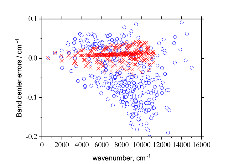
Figure 1: Blue circles: Average ro-vibrational errors for 337 vibrational ($J=0$) states from HITRAN estimated as CO₂ $\tilde{E}^{\rm H}_{\lambda}-\tilde{E}^{\rm T}_{\lambda}$ (HITRAN-TROVE) term values for $J\leq 40$, which were used as band centre corrections (see text). Red crosses: Average residuals for the ro-vibrational CO₂ term values (for $J\leq 40$) between TROVE (before the band centre correction) and calculations from Zak et al. (2016) using DVR3D and the same PES Ames-2016 for 294 vibrational states.

Table 1: Examples of vibrational band centres of CO₂ computed using Ames-2 PES with TROVE ($\tilde{E}^{\rm T}_{\lambda}$), average differences with the HITRAN band centres ($\Delta\tilde{E}_{\lambda}=\tilde{E}^{\rm H}_{\lambda}-\tilde{E}^{\rm T}_{\lambda}$), the shifted band canters adopted for ro-vibrational calculations ($\tilde{E}_{\lambda}^{\rm T}+\Delta\tilde{E}_{\lambda}$) and three sets of quantum numbers (QN) used in this work. See the complete table in supplementary material.

	Linear Molecule QN				HITRAN QN					TROVE QN			Term values (cm-1)
$\lambda$	$n_{1}$	$n_{2}^{\rm lin}$	$l_{2}$	$n_{3}$	$m_{1}$	$m_{2}$	$l_{2}$	$m_{3}$	$r$	$v_{1}$	$v_{2}$	$v_{3}$	$\tilde{E}_{\lambda}^{\rm T}$	$\Delta\tilde{E}_{\lambda}$	$\tilde{E}_{\lambda}^{\rm T}+\Delta\tilde{E}_{\lambda}$
1	0	0	0	0	0	0	0	0	1	0	0	0	0.000	0.000	0.000
2	0	1	1	0	0	1	1	0	1	0	0	0	667.755	0.015	667.769
3	0	2	0	0	1	0	0	0	2	0	0	1	1285.404	0.004	1285.408
4	0	2	2	0	0	2	2	0	1	0	0	0	1336.673	0.020	1336.693
5	1	0	0	0	1	0	0	0	1	1	0	0	1388.209	-0.024	1388.185
6	0	3	1	0	1	1	1	0	2	0	0	1	1932.821	0.039	1932.860
7	0	3	3	0	0	3	3	0	1	0	0	0	2006.732	0.035	2006.766
8	1	1	1	0	1	1	1	0	1	1	0	0	2077.233	0.013	2077.246
9	0	0	0	1	0	0	0	1	1	0	1	0	2349.174	-0.032	2349.141
10	1	2	0	0	2	0	0	0	3	1	0	1	2548.343	0.024	2548.367
11	0	4	2	0	1	2	2	0	2	0	0	1	2586.546	0.039	2586.585
12	2	0	0	0	2	0	0	0	2	1	1	0	2671.144	0.000	2671.144
13	0	4	4	0	0	4	4	0	1	0	0	0	2677.936	0.049	2677.985
14	1	2	2	0	1	2	2	0	1	1	0	0	2762.269	0.018	2762.287
15	1	2	0	0	2	0	0	0	1	1	0	1	2797.157	-0.020	2797.137
16	0	1	1	1	0	1	1	1	1	0	1	0	3004.453	-0.058	3004.395
17	1	3	1	0	2	1	1	0	3	1	0	1	3181.792	0.062	3181.854
18	0	5	3	0	1	3	3	0	2	0	0	1	3244.101	0.045	3244.146
19	2	1	1	0	2	1	1	0	2	1	1	0	3339.706	0.040	3339.746
20	0	5	5	0	0	5	5	0	1	0	0	0	3350.284	0.058	3350.343
21	1	3	3	0	1	3	3	0	1	1	0	0	3445.706	0.030	3445.735
22	1	3	1	0	2	1	1	0	1	1	0	1	3501.033	0.030	3501.063
23	0	2	0	1	1	0	0	1	2	0	1	1	3612.891	-0.052	3612.839
24	0	2	2	1	0	2	2	1	1	0	1	0	3660.884	-0.073	3660.811
25	1	0	0	1	1	0	0	1	1	2	0	0	3714.852	-0.071	3714.781
26	1	4	0	0	3	0	0	0	4	1	0	2	3792.656	0.027	3792.683
27	1	4	2	0	2	2	2	0	3	1	0	1	3823.531	0.046	3823.577
28	0	6	4	0	1	4	4	0	2	0	0	1	3904.544	0.045	3904.589
29	3	0	0	0	3	0	0	0	3	1	2	0	3942.517	0.025	3942.542
30	2	2	2	0	2	2	2	0	2	1	1	0	4009.441	0.035	4009.476
31	0	6	6	0	0	6	6	0	1	0	0	0	4023.775	0.061	4023.836
32	3	0	0	0	3	0	0	0	2	1	2	0	4064.277	-0.002	4064.275
33	1	4	4	0	1	4	4	0	1	1	0	0	4128.500	0.036	4128.536
34	1	4	2	0	2	2	2	0	1	1	0	1	4198.897	0.026	4198.923
35	1	4	0	0	3	0	0	0	1	1	0	2	4225.111	-0.014	4225.097
36	0	3	1	1	1	1	1	1	2	0	1	1	4248.131	-0.044	4248.088
37	0	3	3	1	0	3	3	1	1	0	1	0	4318.455	-0.070	4318.386
38	1	1	1	1	1	1	1	1	1	2	0	0	4391.058	-0.046	4391.012
39	1	5	1	0	3	1	1	0	4	1	0	2	4416.480	0.061	4416.541
40	1	5	3	0	2	3	3	0	3	1	0	1	4470.630	0.034	4470.665
41	0	7	5	0	1	5	5	0	2	0	0	1	4567.381	0.036	4567.417
42	3	1	1	0	3	1	1	0	3	1	2	0	4591.448	0.060	4591.508
43	0	0	0	2	0	0	0	2	1	1	1	0	4673.371	-0.049	4673.322
44	2	3	3	0	2	3	3	0	2	1	1	0	4680.274	0.037	4680.311
45	0	7	7	0	0	7	7	0	1	0	0	0	4698.403	0.055	4698.458
46	3	1	1	0	3	1	1	0	2	1	2	0	4753.794	0.048	4753.841
47	1	5	5	0	1	5	5	0	1	1	0	0	4811.138	0.037	4811.175
48	1	2	0	1	2	0	0	1	3	2	0	1	4853.681	-0.060	4853.622
49	0	4	2	1	1	2	2	1	2	0	1	1	4889.592	-0.062	4889.531
50	1	5	3	0	2	3	3	0	1	1	0	1	4893.567	0.030	4893.597
51	1	5	1	0	3	1	1	0	1	1	0	2	4938.732	0.044	4938.775
52	0	4	4	1	0	4	4	1	1	0	1	0	4977.178	-0.065	4977.113
53	2	0	0	1	2	0	0	1	2	3	0	0	4977.889	-0.056	4977.833
54	1	6	0	0	4	0	0	0	5	1	0	3	5022.354	-0.002	5022.352
55	1	6	2	0	3	2	2	0	4	1	0	2	5048.803	0.023	5048.825
56	1	2	2	1	1	2	2	1	1	2	0	0	5063.368	-0.051	5063.317
57	1	2	0	1	2	0	0	1	1	2	0	1	5099.731	-0.072	5099.659
58	1	6	4	0	2	4	4	0	3	1	0	1	5121.776	0.013	5121.788
59	3	2	0	0	4	0	0	0	4	1	2	1	5197.228	0.026	5197.255
60	0	8	6	0	1	6	6	0	2	0	0	1	5232.314	0.019	5232.333

As an independent benchmark of the TROVE calculations, the initial TROVE energies ($J\leq 40$) before the band centre corrections were compared to the theoretical CO₂ energies computed by Zak et al. (2016) using the DVR3D program (Tennyson et al., 2004) and the same PES as the Ames-2016 line list. Figure 1 shows averaged residuals for 294 bands matched to the CO₂ energy term values from Zak et al. (2016) up to 10 500 cm^-1 with the total rms error of 0.02 cm^-1.

The ro-vibrational energies were computed variationally using the CO₂ empirical PES Ames-2 by Huang et al. (2017) for $J=0\ldots 230$ and used for the temperature partition function of CO₂. The transitional intensities (Einstein A coefficients) were then computed using the UCL ab initio DMS (Polyansky et al., 2015) covering the wavenumber range from 0 to 20 000 cm^-1  with the lower energy term value up to 16 000 cm^-1 ($J\leq 202$). To speed up the calculation of the dipole moment matrix elements, a threshold of $10^{-12}$ to the eigen-coefficients was applied (see Yurchenko et al. (2011)). We have also applied a threshold of $10^{-8}$ Debye to the vibrational matrix elements of the dipole moment in order to reduce an accumulation error for higher overtones, see discussion by Medvedev et al. (2016, 2020).

3 Line list

3.1 Quantum numbers

In TROVE calculations, the ro-vibrational states are uniquely identified by three numbers, the rotational angular momentum quantum number $J$, the total symmetry $\Gamma$ (Molecular symmetry group) and the eigen-state counting number $\lambda$ (in the order of increasing energies). Each state can be further assigned with approximate quantum numbers (QN) associated with the corresponding largest basis set contribution (Yurchenko et al., 2007). There are two main sets of approximate QNs corresponding to the contractions steps 1 and 3. The first set is connected to the primitive basis set excitation numbers $v_{1},v_{2},v_{3}$ and $l_{2}$. The second set is associated with the vibrational counting number $\lambda$ from the ($J=0$)-contracted basis set Eq. (5). Even though $v_{1},v_{2},v_{3}$ and $l_{2}$ are more physically intuitive than the counting number of the vibrational states $\lambda$, the latter is useful for correlating TROVE’s states to the experimental (e.g. normal mode) QNs or indeed to any other scheme. Table 1 shows vibrational ($J=0$) term values of CO₂ together with all assignment schemes either used in these work or relevant to the spectroscopy of CO₂: (i) TROVE primitive QNs $v_{1},v_{2},v_{3}$ and $l$, (ii) TROVE band centres counting number $\lambda$, (iii) HITRAN QNs $m_{1}$, $m_{2}$, $l_{2}$, $m_{3}$, $r$ adopted for CO₂ and (iv) spectroscopic (normal mode) QNs $n_{1}$, $n_{2}^{\rm lin}$, $l_{2}$, $n_{3}$ used for other general linear triatomic molecules. Our preferred choice is (iv). According to this convention, $n_{1}$ and $n_{3}$ are two stretching quantum numbers associated with the symmetric and asymmetric modes; $n_{2}^{\rm lin}$ is the (symmetric) linear molecule bending quantum number; $l_{2}$ is the bending quantum number satisfying the standard conditions on the vibrational angular momentum of an isotropic 2D Harmonic oscillator (Bunker & Jensen, 1998)

$$l_{2}=n_{2}^{\rm lin},n_{2}^{\rm lin}-2,\ldots\,1(0).$$

All ro-vibrational states are automatically assigned the QN schemes (i) and (ii), which were then automatically correlated to the general linear molecule QN (iv) using the following rules:

$$l=l_{2},\quad v_{1}+v_{2}=n_{1}+n_{3},\quad v_{3}=n_{2}^{\rm lin},$$

for a given stretching polyad $n_{1}+n_{2}$, where we assumed that the asymmetric quanta has higher energies than symmetric. For example, for $v_{1}+v_{2}=n_{1}+n_{3}=2$ the stretching QNs ($n_{1},n_{3}$) and assigned to the vibrational term values according with the order of energies: $(2,0)$ 3339.702 cm^-1, $(1,1)$ 3714.853 cm^-1 and $(0,2)$ 4673.392 cm^-1. The linear molecule bending quantum number $n_{2}^{\rm lin}$ is given by

$$n_{2}^{\rm lin}=2v_{3}+l_{2},$$

where $v_{3}$ is the TROVE vibrational bending quantum number. The standard linear molecule QN scheme (iv) was favoured for example by Herzberg & Herzberg (1953) and is also recommended here.

We could not perform similar automatic correlation to the HITRAN quantum labels $(m_{1},m_{2},l_{2},m_{3},r)$ for all the states in our line lists, only for states present in the CO₂ HITRAN database. The HITRAN convention of quantum numbers (iii) for CO₂ is more empirical. It is motivated by energy clusters formed by states in accidental Fermi resonance and their order within a cluster (Rothman & Young, 1981). The quantum number $m_{1}$ is associated with Fermi resonance groups of (symmetric) states of different combinations of $l_{2}$ and $2m_{1}+m_{2}=2n_{1}+n_{2}^{\rm lin}$; $r$ is the ranking index, with $r=1$ for the highest vibrational level of a Fermi resonance group and assuming the values $1,2,\ldots m_{1}+1$ (Rothman & Young, 1981). HITRAN’s version of the bending quantum number $m_{2}$ is by definition equal to $l_{2}$ (so-called AFGL notation) and thus redundant, while the stretching quantum number $m_{3}$ is the same as the linear molecule asymmetric quantum number $n_{3}$ from scheme (iv). In order to simplify correlation with HITRAN and experimental literature, the scheme (iii) is retained, but only for the ro-vibrational states present in HITRAN.

4 Line list

The CO₂  UCL-4000 line list contains 3 480 477 states and 2 557 551 923 transitions and covers the wavenumber range from 0 to 20 000 cm^-1  (wavelengths, $\lambda>0.5$ $\mu$m) with the lower energy up to 16 000 cm^-1 and $J\leq 202$ with a threshold on the Einstein coefficients of $10^{-14}$ s^-1. The line list consists of two files (Tennyson et al., 2016), called States and Transitions, which in the case of UCL-4000 are summarised in Tables 2 and 3. The first 4 columns of the States file have the compulsory structure for all molecules: State ID, Energy term value (cm^-1), the total degeneracy and the total angular momentum. According to the new ExoMol-2020 format (Tennyson et al., 2020), the 5th column is also compulsory representing the uncertainty estimate of the corresponding term value (cm^-1), which is followed by the lifetime, Landé $g$-factor (if provided) and molecular specific quantum numbers, including rigorous (symmetry, parity) and non-rigorous (vibrational, rotational, etc). The States file covers all states up to $J=230$ (3 526 057 states). The Transitions part consists of three columns with the upper State ID, lower State ID and the Einstein $A$ coefficient, see Table 3. For convenience, the Transition part is split into 20 files each covering 1000 cm^-1.

Table 2: Extracts from the final states file for UCL-4000.

$i$	$\tilde{E}$	$g_{\rm tot}$	$J$	unc.	$\Gamma$	$e/f$	$n_{1}$	$n_{2}^{\rm lin}$	$l_{2}$	$n_{3}$	$C_{i}$	$m_{1}$	$m_{2}$	$m_{3}$	$m_{4}$	$r$	$v_{1}^{\rm T}$	$v_{2}^{\rm T}$	$v_{3}^{\rm T}$
1	0.000000	1	0	0.0005	A1	e	0	0	0	0	1.00	0	0	0	0	1	0	0	0
2	1285.408200	1	0	0.0005	A1	e	0	2	0	0	1.00	1	0	0	0	2	0	0	1
3	1388.184200	1	0	0.0050	A1	e	1	0	0	0	1.00	1	0	0	0	1	1	0	0
4	2548.366700	1	0	0.0005	A1	e	1	2	0	0	1.00	2	0	0	0	3	1	0	1
5	2671.142957	1	0	0.0050	A1	e	2	0	0	0	1.00	2	0	0	0	2	1	1	0
6	2797.136000	1	0	0.0050	A1	e	1	2	0	0	1.00	2	0	0	0	1	1	0	1
7	3792.681898	1	0	0.0050	A1	e	1	4	0	0	1.00	3	0	0	0	4	1	0	2
8	3942.541358	1	0	0.0050	A1	e	3	0	0	0	1.00	3	0	0	0	3	1	2	0
9	4064.274256	1	0	0.0050	A1	e	3	0	0	0	1.00	3	0	0	0	2	1	2	0
10	4225.096148	1	0	0.0050	A1	e	1	4	0	0	1.00	3	0	0	0	1	1	0	2
11	4673.325200	1	0	0.0005	A1	e	0	0	0	2	1.00	0	0	0	2	1	1	1	0
12	5022.349428	1	0	0.0050	A1	e	1	6	0	0	1.00	4	0	0	0	5	1	0	3
13	5197.252900	1	0	0.0050	A1	e	3	2	0	0	1.00	4	0	0	0	4	1	2	1
14	5329.645446	1	0	0.0050	A1	e	4	0	0	0	1.00	4	0	0	0	3	2	2	0
15	5475.553054	1	0	0.0005	A1	e	3	2	0	0	1.00	4	0	0	0	2	1	2	1
16	5667.644584	1	0	0.0050	A1	e	2	4	0	0	1.00	4	0	0	0	1	1	1	2
17	5915.212302	1	0	0.0005	A1	e	0	2	0	2	1.00	1	0	0	2	2	1	1	1
18	6016.690121	1	0	0.0005	A1	e	1	0	0	2	1.00	1	0	0	2	1	0	3	0
19	6240.044061	1	0	0.08	A1	e	2	6	0	0	1.00	-1	-1	-1	-1	-1	1	1	3
20	6435.507278	1	0	0.06	A1	e	4	2	0	0	1.00	-1	-1	-1	-1	-1	2	2	1
21	6588.323819	1	0	0.05	A1	e	5	0	0	0	1.00	-1	-1	-1	-1	-1	3	2	0

$i$: State counting number.

$\tilde{E}$: State energy in cm^-1.

$g_{\rm tot}$: Total state degeneracy.

$J$: Total angular momentum.

unc.: Uncertainty cm^-1: The empirical (4 decimal places) and estimated (2 decimal places) values.

$\Gamma$: Total symmetry index in ${\mathcal{C}}_{2{\rm v}}$(M)

$e/f$: Kronig rotationless parity

$n_{1}$: Normal mode stretching symmetry ($A_{1}$) quantum number.

$n_{2}^{\rm lin}$ : Normal mode linear molecule bending ($A_{1}$) quantum number.

$l_{2}$: Normal mode vibrational angular momentum quantum number.

$n_{3}$: Normal mode stretching asymmetric ($B1_{1}$) quantum number.

$C_{i}$: Coefficient with the largest contribution to the $(J=0)$ contracted set; $C_{i}\equiv=1$ for $J=0$.

$m_{1}$: CO₂ symmetric vibrational Fermi-resonance group quantum number (-1 stands for non available).

$m_{2}$: CO₂ vibrational bending quantum number (similar but not exactly identical to $n_{2}^{\rm lin}$).

$l_{2}$: CO₂ vibrational bending quantum number (similar but not exactly identical to standard $l_{2}$).

$m_{3}$: CO₂ asymmetric vibrational stretching quantum number, the same as $n_{3}$.

$r$: CO₂ additional ranking quantum number identifying states within a Fermi-resonance group.

$v_{1}^{\rm T}$: TROVE stretching vibrational quantum number.

$v_{2}^{\rm T}$: TROVE stretching vibrational quantum number.

$v_{3}^{\rm T}$: TROVE bending vibrational quantum number.

Table 3: Extract from the transitions file for the UCL-4000 line list.

$f$	$i$	$A_{fi}$
1176508	1137722	2.8564E-02
1861958	1849078	1.6327E-03
631907	665295	8.1922E-12
1344897	1331267	4.2334E-07
983465	944281	1.4013E-08
183042	170520	1.6345E-02
2695389	2668685	5.9366E-07
811518	822542	1.4353E-01
406949	369902	2.3774E-02

$f$: Upper state counting number.
$i$: Lower state counting number.
$A_{fi}$: Einstein-A coefficient in s^-1.

The uncertainty of the CO₂ energies were estimated based on the two main criteria. For the states matched to and replaced by the HITRAN energies, the uncertainties $\sigma$ (in cm^-1) are taken as the HITRAN errors of the corresponding line positions as specified by the HITRAN error codes (Rothman et al., 2005). For all other states the following conservative estimate is used:

$$\sigma=0.01\,n_{1}+0.01\,n_{2}^{\rm lin}+0.01\,n_{3}.$$

With the lower state energy threshold of 16 000 cm^-1 our line list should be valid for temperatures up to at least 2500 K. Figure 2 (left) illustrates the effect of the lack of the population for the states higher than 16 000 cm^-1 with the help of the CO₂ partition function $Q(T)$. In this figure we show a ratio of incomplete $Q^{E_{\rm max}}(T)$ (using only states below $E_{\rm max}$) over ‘complete’ $Q^{36000}$(T). This ratio has the difference of 2 % for $Q^{16000}$ at $T=$ 2500 K and $Q^{26000}$ at $T=$ 4000 K, which are the estimates for maximal temperature of the line list for wavenumber regions 0–20 000 cm^-1 and 10 000–20 000 cm^-1, respectively. In Figure 2 (right) we compare the partition functions of CO₂ computed using our line list with the Total Internal Partition Sums (TIPS) values for CO₂ (Gamache et al., 2017). The energies in our line list cover higher rotational excitations ($J_{\rm max}$ = 230) compared to TIPS, which was based on the threshold of $J_{\rm max}=150$. The energy thresholds in both cases are comparable, $hc\cdot$36 000 cm^-1 vs $hc\cdot$30 383 cm^-1 (TIPS). The threshold value of $J_{\rm max}=150$ corresponds the energy term value of $\sim$ 10 000 cm^-1and thus leads the underestimate of the partition function of high $T$, while with the threshold of $J_{\rm max}$ = 230 all states below 20 000 cm^-1 are included.

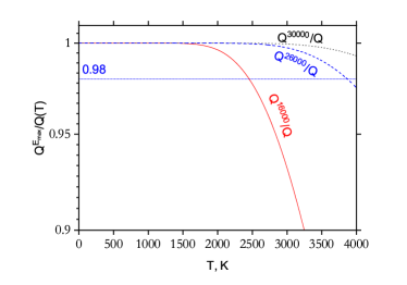
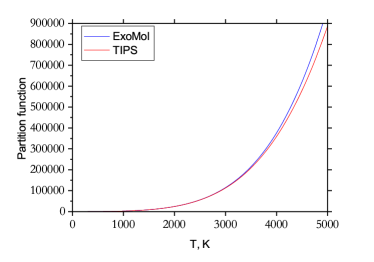
Figure 2: Partition functions of CO₂. Left display: Ratio $Q^{E_{\rm max}}(T)/Q(T)$ of the CO₂ partition functions at with energy cutoffs $hc\cdot$16 000 cm^-1, $hc\cdot$26000 cm^-1 and $hc\cdot$30000 cm^-1, as a function of temperature. $Q(T)$ is chosen as $Q^{36000~{}{\rm cm}^{-1}}$. The line $0.98$ shows that the recommended temperature varies with the wavenumber region, from $T=$ 2500 K ($>$ 0 cm^-1) to $T=$ 4000 K ($>$ 10 000 cm^-1). Right display: ExoMol values were computed using all UCL-4000 energies for $J\leq 230$; TIPS values were obtained using the TIPS app provided in Gamache et al. (2017).

In order to improve the calculated line positions, CO₂ energies from HITRAN were used to replace the TROVE energies where available, taking advantage of the two-part structure of the UCL-4000 line list consisting of a States file and Transition files (Tennyson et al., 2016). A HITRAN energy list consisting of 18 392 empirical values from 337 vibrational states covering $J$ values up to 129 was generated by collecting all lower and upper state energies from the ¹²C¹⁶O₂ HITRAN transitions. Comparison of the calculated TROVE term energies with these 18 668 HITRAN values gives an rms error of 0.016 cm^-1 and is illustrated in Fig. 3 in a log-scale.

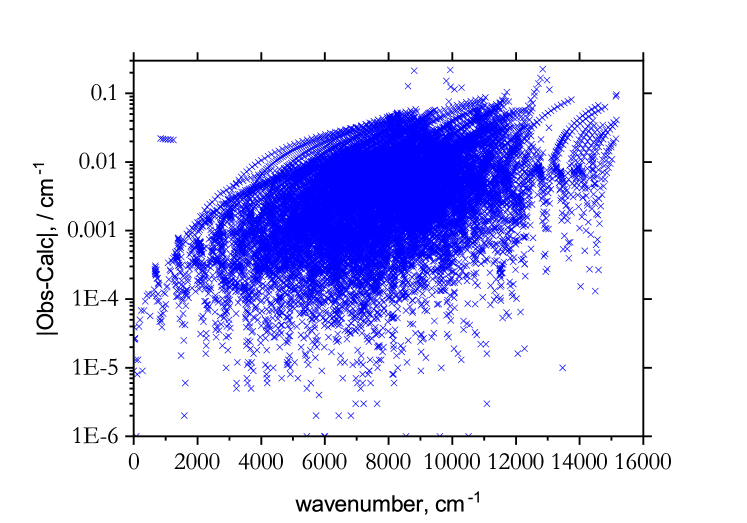
Figure 3: Ro-vibrational Obs.-Calc. errors $|\tilde{E}_{i}^{\rm H}-\tilde{E}_{i}^{\rm T}|$ (HITRAN-TROVE) in cm^-1 for all HITRAN’s 18 392 empirical values as a function of the energy term values, covering $J\leq 129$ giving an rms error of 0.016 cm^-1.

The overview of the CO₂ absorption spectrum and its temperature dependence are illustrated in Fig. 4. CO₂ has a prominent band at 4.3 $\mu$m, commonly used for atmospheric and astrophysical retrievals. For example, it was used as one of the photometric bands for the Spitzer Space Telescope (Werner et al., 2004).

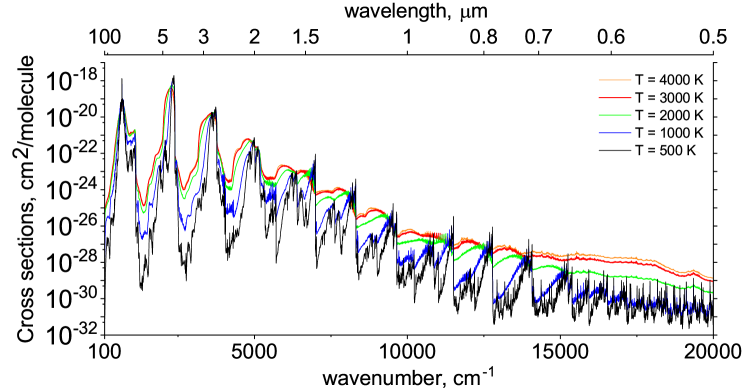
Figure 4: Temperature dependence of the CO₂ spectrum using the Gaussian line profile of HWHM=1 cm^-1. The spectrum becomes systematically flatter with increasing temperature.

Our line list is designed to almost perfectly agree with the HITRAN line positions, which was achieved by replacing the TROVE energies with the energies collected from the HITRAN data set for CO₂. Figures 5 and 6 offer some comparisons with HITRAN. In turn, the accuracy of the line intensities agree well with the HITRAN values as guaranteed by the quality of the UCL ab initio DMS used. The mean ratio of our intensities to HITRAN is 1.0029 with the standard error of 0.00029 for 171143 HITRAN lines we could establish a correlation to.

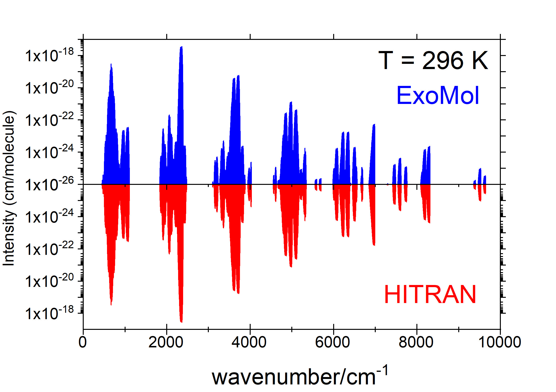
Figure 5: CO₂  stick spectrum comparing using UCL-4000 to HITRAN at $T=296$ K.

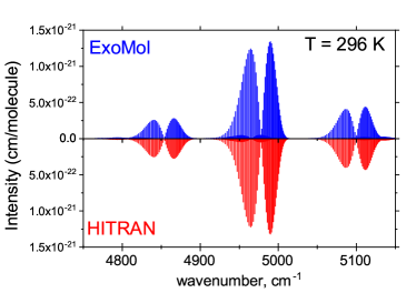
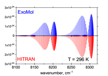
Figure 6: Absorption stick spectrum of CO₂ computed using UCL-4000 and compared to HITRAN at $T=296$ K for two spectroscopic regions.

Figure 7 compares the performance of the four main line lists for hot CO₂, UCL-4000 (this work), CDSD-4000 (effective Hamiltonian) (Tashkun & Perevalov, 2011), Ames-2 (variational) (Huang et al., 2017) and 2010 HITEMP (empirical) (Rothman et al., 2010) for the wavenumber range from 0 to 15 000 cm^-1. In general the UCL-4000 line list gives the highest opacity at $T=4000$ K which is due to its being more complete, while both CDSD-4000 and 2010 HITEMP omit too many hot bands to be able to compete with the other two line lists at high $T$. The Ames-2016 line list also lacks a significant portion of the opacity at short wavelengths at this temperature as expected from the low energy threshold used (Huang et al., 2017).

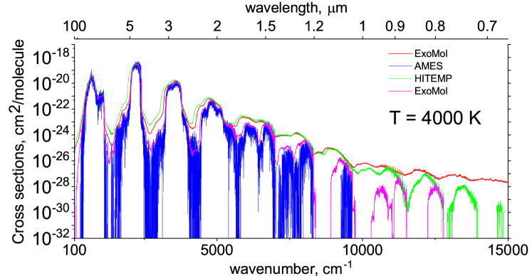
Figure 7: Comparing UCL-4000, CDSD-4000 (Tashkun & Perevalov, 2011), Ames-2016 (Huang et al., 2017) and 2010 HITEMP (Rothman et al., 2010) spectra of CO₂ at $T=4000$ K. A Gaussian line profile of HWHM=1 cm^-1 was used in each case.

Figure 8 compares the UCL-4000 spectrum of CO₂ at $T=1773$ K with the experiment by Evseev et al. (2012), who recorded transmittance of CO₂ at the normal pressure. The displays on the left show small windows from the two strongest CO₂ bands, 2.7 $\mu$m and 4.3 $\mu$m at higher resolution, while the displays on the right gives an overview of the whole region covering these bands at lower resolution. As a reference, spectra computed with the 2010 HITEMP line list are also shown. At this temperature, UCL-4000 performs very similarity to 2010 HITEMP and shows excellent agreement with the experiment.

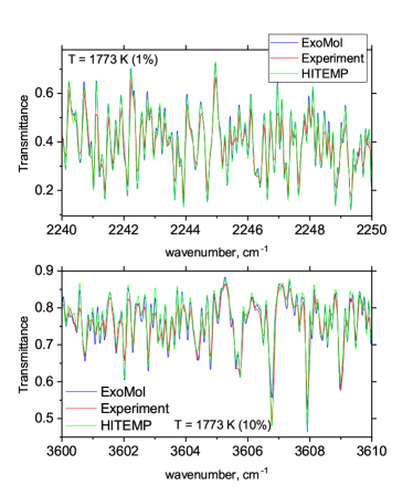
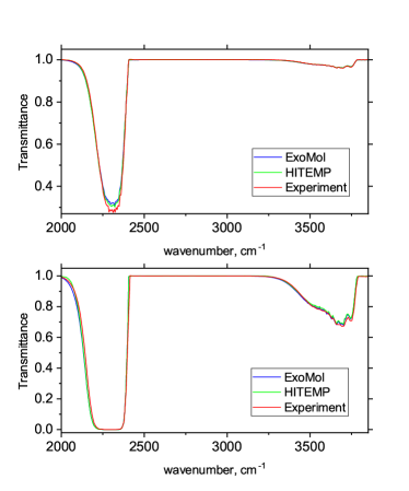
Figure 8: Comparing HITEMP and ExoMol to experimental transmittance (Evseev et al., 2012) at $T=1773$ K and 1 bar using a Voigt profile. The experiments were performed with 1% (upper) and 10% (lower) CO₂ in N₂ buffer gas. HITEMP line width parameters were used for HITEMP, while for UCL-4000 we used an approximate scheme a0 from the ExoMol diet (Barton et al., 2017) based on the HITRAN values. The left display shows two selected windows at high resolution (0.0125 cm^-1), while the right display is with broader overview and lower resolution (6 cm^-1).

5 Conclusion

A new hot line list for the main isotopologue of CO₂ (¹²C¹⁶O₂) is presented, which is the most comprehensive (complete and accurate) data set for carbon dioxide to date. The line list is an important addition to the ExoMol database which now contains line lists for all the major constituents of hot Jupiter and mini-Neptune exoplanets. Line lists are still being added to address the problem of hot super Earth exoplanets, or lava planets, the composition of whose atmospheres are currently not well constrained.

The line lists can be downloaded from the CDS (http://cdsweb.u-strasbg.fr/) or from ExoMol (www.exomol.com databases.

Data availability statement

Full data is made available. The line lists can be downloaded from the CDS (http://cdsweb.u-strasbg.fr/) or from ExoMol (www.exomol.com databases.

The complete list of the band centres and their corrections is given as supplementary material to the paper

References

- Barton et al. (2017) Barton E. J., Hill C., Czurylo M., Li H.-Y., Hyslop A., Yurchenko S. N., Tennyson J., 2017, J. Quant. Spectrosc. Radiat. Transf., 203, 490
- Baylis-Aguirre et al. (2020) Baylis-Aguirre D. K., Creech-Eakman M. J., Güth T., 2020, MNRAS, 493, 807
- Bunker & Jensen (1998) Bunker P. R., Jensen P., 1998, Molecular Symmetry and Spectroscopy, 2nd edn. NRC Research Press, Ottawa
- Carter et al. (1983) Carter S., Handy N., Sutcliffe B., 1983, Mol. Phys., 49, 745
- Chubb et al. (2020) Chubb K. L., Tennyson J., Yurchenko S. N., 2020, MNRAS, 493, 1531
- Connor et al. (2016) Connor B. et al., 2016, Atmos. Meas. Tech., 9, 5227
- Cooley (1961) Cooley J. W., 1961, Math. Comp., 15, 363
- Evseev et al. (2012) Evseev V., Fateev A., Clausen S., 2012, J. Quant. Spectrosc. Radiat. Transf., 113, 2222
- Gamache et al. (2017) Gamache R. R. et al., 2017, J. Quant. Spectrosc. Radiat. Transf., 203, 70
- Gordon & et al. (2017) Gordon I. E., et al., 2017, J. Quant. Spectrosc. Radiat. Transf., 203, 3
- Heng & Lyons (2016) Heng K., Lyons J. R., 2016, ApJ, 817, 149
- Herzberg & Herzberg (1953) Herzberg G., Herzberg L., 1953, J. Opt. Soc. Am., 43, 1037
- Hougen et al. (1970) Hougen J. T., Bunker P. R., Johns J. W. C., 1970, J. Mol. Spectrosc., 34, 136
- Huang et al. (2013) Huang X., Freedman R. S., Tashkun S. A., Schwenke D. W., Lee T. J., 2013, J. Quant. Spectrosc. Radiat. Transf., 130, 134
- Huang et al. (2014) Huang X., Gamache R. R., Freedman R. S., Schwenke D. W., Lee T. J., 2014, J. Quant. Spectrosc. Radiat. Transf., 147, 134
- Huang et al. (2017) Huang X., Schwenke D. W., Freedman R. S., Lee T. J., 2017, J. Quant. Spectrosc. Radiat. Transf., 203, 224
- Huang et al. (2019) Huang X., Schwenke D. W., Lee T. J., 2019, J. Quant. Spectrosc. Radiat. Transf., 230, 222
- Huang et al. (2012) Huang X., Schwenke D. W., Tashkun S. A., Lee T. J., 2012, J. Chem. Phys., 136, 124311
- Kang et al. (2018) Kang P., Wang J., Liu G.-L., Sun Y. R., Zhou Z.-Y., Liu A.-W., Hu S.-M., 2018, J. Quant. Spectrosc. Radiat. Transf., 207, 1
- Long et al. (2020) Long D., Reed Z., Fleisher A., Mendonca J., Roche S., Hodges J., 2020, Geophys. Res. Lett., 47, e2019GL086344
- Massol et al. (2016) Massol H. et al., 2016, Space Sci. Rev., 205, 153
- Medvedev et al. (2016) Medvedev E. S., Meshkov V. V., Stolyarov A. V., Ushakov V. G., Gordon I. E., 2016, J. Mol. Spectrosc., 330, 36
- Medvedev et al. (2020) Medvedev E. S., Ushakov V. G., Conway E. K., Upadhyay A., Gordon I. E., Tennyson J., 2020, J. Quant. Spectrosc. Radiat. Transf., 252, 107084
- Moses et al. (2013) Moses J. I., Madhusudhan N., Visscher C., Freedman R. S., 2013, ApJ, 763, 25
- Noumerov (1924) Noumerov B. V., 1924, MNRAS, 84, 592
- Odintsova et al. (2017) Odintsova T., Fasci E., Moretti L., Zak E. J., Polyansky O. L., Tennyson J., Gianfrani L., Castrillo A., 2017, J. Chem. Phys., 146, 244309
- Oyafuso et al. (2017) Oyafuso F. et al., 2017, J. Quant. Spectrosc. Radiat. Transf., 203, 213
- Polyansky et al. (2015) Polyansky O. L., Bielska K., Ghysels M., Lodi L., Zobov N. F., Hodges J. T., Tennyson J., 2015, Phys. Rev. Lett., 114, 243001
- Rein & Sanders (2010) Rein K. D., Sanders S. T., 2010, Appl. Optics, 49, 4728
- Rothman et al. (2010) Rothman L. S. et al., 2010, J. Quant. Spectrosc. Radiat. Transf., 111, 2139
- Rothman et al. (2005) Rothman L. S. et al., 2005, J. Quant. Spectrosc. Radiat. Transf., 96, 139
- Rothman & Young (1981) Rothman L. S., Young L. D., 1981, J. Quant. Spectrosc. Radiat. Transf., 25, 505
- Snels et al. (2014) Snels M., Stefani S., Grassi D., Piccioni G., Adriani A., 2014, Planet Space Sci., 103, 347
- Sutcliffe & Tennyson (1991) Sutcliffe B. T., Tennyson J., 1991, Int. J. Quantum Chem., 39, 183
- Swain et al. (2010) Swain M. R. et al., 2010, Nature, 463, 637
- Swain et al. (2009a) Swain M. R. et al., 2009a, ApJ, 704, 1616
- Swain et al. (2009b) Swain M. R., Vasisht G., Tinetti G., Bouwman J., Chen P., Yung Y., Deming D., Deroo P., 2009b, ApJL, 690, L114
- Tashkun & Perevalov (2011) Tashkun S. A., Perevalov V. I., 2011, J. Quant. Spectrosc. Radiat. Transf., 112, 1403
- Tashkun et al. (2003) Tashkun S. A., Perevalov V. I., Teffo J. L., Bykov A. D., Lavrentieva N. N., 2003, J. Quant. Spectrosc. Radiat. Transf., 82, 165
- Tennyson et al. (2004) Tennyson J., Kostin M. A., Barletta P., Harris G. J., Polyansky O. L., Ramanlal J., Zobov N. F., 2004, Comput. Phys. Commun., 163, 85
- Tennyson & Yurchenko (2012) Tennyson J., Yurchenko S. N., 2012, MNRAS, 425, 21
- Tennyson et al. (2020) Tennyson J. et al., 2020, J. Quant. Spectrosc. Radiat. Transf.
- Tennyson et al. (2016) Tennyson J. et al., 2016, J. Mol. Spectrosc., 327, 73
- Vargas et al. (2020) Vargas J., Lopez B., da Silva M. L., 2020, J. Quant. Spectrosc. Radiat. Transf., 245, 106848
- Čermák et al. (2018) Čermák P., Karlovets E. V., Mondelain D., Kassi S., Perevalov V. I., Campargue A., 2018, J. Quant. Spectrosc. Radiat. Transf., 207, 95
- Wattson & Rothman (1992) Wattson R. B., Rothman L. S., 1992, J. Quant. Spectrosc. Radiat. Transf., 48, 763
- Werner et al. (2004) Werner M. W. et al., 2004, ApJS, 154, 1
- Yurchenko et al. (2011) Yurchenko S. N., Barber R. J., Tennyson J., 2011, MNRAS, 413, 1828
- Yurchenko & Mellor (2020) Yurchenko S. N., Mellor T. M., 2020, J. Chem. Phys., submitted
- Yurchenko et al. (2007) Yurchenko S. N., Thiel W., Jensen P., 2007, J. Mol. Spectrosc., 245, 126
- Yurchenko et al. (2017) Yurchenko S. N., Yachmenev A., Ovsyannikov R. I., 2017, J. Chem. Theory Comput., 13, 4368
- Zak et al. (2016) Zak E. J., Tennyson J., Polyansky O. L., Lodi L., Tashkun S. A., Perevalov V. I., 2016, J. Quant. Spectrosc. Radiat. Transf., 177, 31
- Zak et al. (2017a) Zak E. J., Tennyson J., Polyansky O. L., Lodi L., Zobov N. F., Tashkun S. A., Perevalov V. I., 2017a, J. Quant. Spectrosc. Radiat. Transf., 203, 265
- Zak et al. (2017b) Zak E. J., Tennyson J., Polyansky O. L., Lodi L., Zobov N. F., Tashkun S. A., Perevalov V. I., 2017b, J. Quant. Spectrosc. Radiat. Transf., 189, 267