Markovian approximation of the rough Bergomi model for Monte Carlo option pricing

Abstract

The recently developed rough Bergomi (rBergomi) model is a rough fractional stochastic volatility (RFSV) model which can generate more realistic term structure of at-the-money volatility skews compared with other RFSV models. However, its non-Markovianity brings mathematical and computational challenges for model calibration and simulation. To overcome these difficulties, we show that the rBergomi model can be approximated by the Bergomi model, which has the Markovian property. Our main theoretical result is to establish and describe the affine structure of the rBergomi model. We demonstrate the efficiency and accuracy of our method by implementing a Markovian approximation algorithm based on a hybrid scheme.

Keywords: rough fractional stochastic volatility, forward variance model, Markovian representation, volatility skew, Volterra integral, rough Heston, hybrid scheme simulation

MSC codes: 60H35; 65C30; 91G20; 91G60; 65C05; 62P05; JEL codes: C63; C15; C52; G13; G12; C02
ACM codes: G.3; I.6.1; F.2.1; G.1.2; I.6.3; G.1.10;

1 Introduction

The rough Bergomi (rBergomi) model introduced by Bayer et al., (2016) has gained acceptance for stochastic volatility modelling due to its power-law at-the-money volatility skew which is consistent with empirical studies (see Forde and Zhang, 2017, Fukasawa, 2017, Gatheral et al., 2018) and the market impact function under the no-arbitrage assumption (see Jusselin and Rosenbaum, 2018). However, the stochastic process which characterizes this volatility model is rougher than that of a Brownian motion; in particular, the lack of Markovianity makes classical pricing methods infeasible.

In order to price options under an rBergomi model and calibrate such a model, Bayer et al., (2018) propose hierarchical adaptive sparse grids for option pricing, Bayer et al., (2019) propose a deep learning method for rBergomi model calibration, Jacquier et al., (2018) develop pricing algorithms for VIX futures and options, and McCrickerd and Pakkanen, (2018) develop a ‘turbocharged’ Monte Carlo pricing method. In spite of these efforts, the inherent challenges brought by the rBergomi model still prevent its widespread adoption in industry.

Inspired by the technique from Abi Jaber and El Euch, (2019), Gatheral and Keller-Ressel, (2019) and Harms and Stefanovits, (2019), in which the authors design a multi-factor stochastic volatility model with Markovian structure to approximate the rough Heston model, we establish an analogous multi-factor affine structure for the rBergomi model. In the affine structure, the Volterra kernel corresponds to a superposition of infinitely many Ornstein-Uhlenbeck (O-U) processes with different speeds of mean reversion. Truncating this infinite sum into a finite sum of O-U processes yields an approximation of the rBergomi model which is a Markovian approximated Bergomi (aBergomi) model. We then prove the existence and uniqueness of solutions to this affine aBergomi model, and show that its affine structure converges to the one of the rBergomi model.

To numerically simulate the rBergomi model in practice, we adopt the hybrid scheme proposed in Bennedsen et al., (2017) for the stochastic Volterra-type integrals $\tilde{X}=\sqrt{2\alpha+1}\int_{s}^{t}(t-s)^{\alpha}dW_{s}$ ($\kappa=1$). The hybrid scheme consists in approximating the power-law kernel $K_{\text{pow}}=\sqrt{2\alpha+1}(t-s)^{\alpha}$ by a combination of a power function near zero and a step function elsewhere, with a lower $\mathcal{O}(N\log N)$ complexity, where $N$ is the number of time steps, as opposed to the $\mathcal{O}(N^{3})$ complexity of the Cholesky method in Bayer et al., (2016). Here, the rBergomi power-law kernel $K_{\text{pow}}$ can be approximated by the exponential kernel $K_{\text{exp}}=\sum_{i=1}^{n}\alpha_{i}e^{-\kappa_{i}(t-s)}$ after truncating $K_{\text{pow}}$ before $t$. Our numerical tests demonstrate that using $n=25$ exponential terms in $K_{\text{exp}}$ (i.e. a 25-term O-U process), we can obtain an accurate (low root mean squared error), yet tractable and computationally efficient approximation of the fractional rBergomi model.

The paper is organized as follows. In Section 2, we introduce the Bergomi and rBergomi models and discuss their respective ATM volatility skews. In particular we provide for the first time a proof that the ATM volatility skew of the rBergomi model is equivalent to the power $T^{H-\frac{1}{2}}$ while this does not hold for the Bergomi model (equation (8)). In Section 3, we establish the affine structure of the rough Bergomi model. Section 4 is dedicated to the approximation of the rough Bergomi model by a multi-factor Bergomi model. Finally, Section 5 compares numerical simulations of the rBergomi model with our approximated Bergomi (aBergomi) model with a finite number of terms, showing the effectiveness of our approximation.

2 Bergomi and rough Bergomi models

This section introduces the Bergomi and rough Bergomi stochastic volatility models (Definitions 2 and 1), along with the corresponding notations used throughout the paper.

We consider a filtered probability space $(\Omega,\mathcal{F},(\mathcal{F}_{t})_{t\in\mathbb{R}},\mathbb{Q})$, which supports two dimensional correlated Brownian motions $W$ and $B$. A log price process $X_{t}:=\log(S_{t})$ is assumed to follow the dynamics

$$dX_{t}=-\frac{1}{2}V_{t}dt+\sqrt{V_{t}}dW_{t}\,,$$ (1)

where $V_{t}\geq 0$ is the instantaneous spot variance process. Let $\xi_{t}^{u},u\geq t$ be the instantaneous forward variance for date $u$ observed at time $t$; in particular $\xi_{t}^{t}=V_{t}$ corresponds to the spot variance.

Bayer et al., (2016) proposed the so-called rough Bergomi model where the forward variance follows

$$d\xi_{t}^{u}=\xi_{t}^{u}\eta\sqrt{2\alpha+1}\left(u-t\right){}^{\alpha}dB_{t},~{}u\geq t$$ (2)

where $W$ and $B$ have correlation $\rho$, $\alpha\triangleq H-\frac{1}{2}\in\left(-\frac{1}{2},0\right)$ is a negative exponent depending on the Hurst exponent $H\in\left(0,\frac{1}{2}\right)$ of the underlying fractional Brownian motion, and $\eta$ is a positive parameter depending on $H$. The definition of the rBergomi model is summarized below:

Definition 1.

The rBergomi stochastic volatility model takes the form

$$\left\{\begin{aligned} &dX_{t}=-\frac{1}{2}V_{t}dt+\sqrt{V_{t}}dW_{t},\\ &d\xi_{t}^{u}=\xi_{t}^{u}\eta\sqrt{2\alpha+1}(u-t)^{\alpha}dB_{t},\end{aligned}\right.$$ (3)

where $\alpha=H-\frac{1}{2}\in\left(-\frac{1}{2},0\right)$, and $d\left\langle W,B\right\rangle_{t}=\rho dt$.

By contrast, the two-factor Bergomi model is defined as follows.

Definition 2.

The two-factor Bergomi model (Bergomi, 2005, Bergomi, 2009) is defined by:

$$\left\{\begin{aligned} &dX_{t}=-\frac{1}{2}V_{t}dt+\sqrt{V_{t}}dW_{t}^{S},\\ &d\xi_{t}^{u}=\xi_{t}^{u}\alpha_{\theta}\omega\left(\left(1-\theta\right)e^{-\kappa_{X}(u-t)}dW_{t}^{X}+\theta e^{-\kappa_{Y}(u-t)}dW_{t}^{Y}\right)\end{aligned}\right.$$ (4)

with

$$d\langle W^{S},W^{X}\rangle_{t}=\rho_{SX}dt$$

$$d\langle W^{S},W^{Y}\rangle_{t}=\rho_{SY}dt$$

$$d\langle W^{X},W^{Y}\rangle_{t}=\rho_{XY}dt,$$

where $\xi_{t}^{t}=V_{t}=\omega$ is the lognormal volatility of the instantaneous variance under the normalizing factor $\alpha_{\theta}=\left(\left(1-\theta\right){}^{2}+2\rho_{XY}\theta\left(1-\theta\right)+\theta^{2}\right){}^{-\frac{1}{2}}$ and $\theta$ is a mixing parameter of the short term factor driven by $W^{X}$ and the long term factor driven by $W^{Y}$ ($\kappa_{X}>\kappa_{Y}$).

Assumption 1.

Without loss of generality, we assume throughout the paper that the initial forward variance curve $\xi_{0}^{u},u\geq 0$ is flat. This simplification is common in the rBergomi literature, see for example Bayer et al., (2016), Bayer et al., (2018) and Bayer et al., (2019). We use the notation $\xi_{0}$ for the constant initial forward variance curve.

2.1 ATM volatility skew

This subsection derives the ATM volatility skew of the rBergomi and Bergomi models, as the more realistic ATM volatility skew of the rBergomi model over the Bergomi model is one of the motivations behind the introduction of the rBergomi model.

From Bergomi and Guyon, (2012), we can define the price and the volatility dynamics of a generic stochastic volatility model as follows:

$$\left\{\begin{aligned} &dX_{t}=-\frac{1}{2}V_{t}dt+\sqrt{V_{t}}dW_{t}\\ &d\xi_{t}^{u}=\lambda(t,u,\xi_{t}^{u})dB_{t},\end{aligned}\right.$$ (5)

where in particular note that $X_{t}=\xi_{t}^{t}=\ln(S_{t})$ is the log-spot, $V_{t}$ is the instantaneous spot variance, $\xi_{t}^{u}$ is the instantaneous forward variance for date $u$ observed at time $t$, and $\lambda=(\lambda_{1},\cdots,\lambda_{d})$ is the volatility of forward instantaneous variances which takes values in $\mathbb{R}^{d}$ where $d$ is the dimension of the Brownian motion $B$. Note that in this formulation, the covariance between spot and variance is modelled through the first component of $\lambda$, see Bergomi and Guyon, (2012) for more details.

One can derive the following second-order expression (w.r.t. volatility of volatility) for the Black-Scholes implied volatility:

$$\sigma_{BS}(k,T)=\hat{\sigma}_{T}^{ATM}+\mathcal{S}_{T}k+\mathcal{C}_{T}k^{2}+\mathcal{O}(\varepsilon^{3})\,,$$ (6)

where $k=\ln\left(\frac{K}{S_{0}}\right)$, $K$ is the strike and $\varepsilon$ is a dimensionless scaling factor for the volatility of variances. The ATM volatility and the two coefficients $\mathcal{S}_{T}$ and $\mathcal{C}_{T}$ are given by

$$\hat{\sigma}_{T}^{ATM} =\hat{\sigma}_{T}^{VS}\left[1+\frac{\varepsilon}{4v}C^{X\xi}+\frac{\varepsilon^{2}}{32v^{3}}\left(12\left(C^{X\xi}\right){}^{2}-v(v+4)C^{\xi\xi}+4v(v-4)C^{\mu}\right)\right],$$

$$\mathcal{S}_{T} =\hat{\sigma}_{T}^{VS}\left[\frac{\varepsilon}{2v^{2}}C^{X\xi}+\frac{\varepsilon^{2}}{8v^{3}}\left(4C^{\mu}v-3(C^{X\xi})^{2}\right)\right],$$

$$\mathcal{C}_{T} =\hat{\sigma}_{T}^{VS}\frac{\varepsilon^{2}}{8v^{4}}\left[4C^{\mu}v+C^{\xi\xi}v-6\left(C^{X\xi}\right){}^{2}\right]$$

where $v=\int_{0}^{T}\xi_{0}^{s}ds$ is the total variance to expiration $T$, $\hat{\sigma}_{T}^{VS}=\sqrt{\frac{v}{T}}=\sqrt{\frac{\int_{0}^{T}\xi_{0}^{s}ds}{T}}$ is the effective volatility, and $C^{X\xi},~{}C^{\xi\xi},~{}C^{\mu}$ are autocorrelations (Bergomi and Guyon,, 2012):

• $C_{t}^{X\xi}(\xi)=\int_{t}^{T}ds\int_{s}^{T}du\mu\left(s,u,\xi\right)=\int_{t}^{T}ds\int_{s}^{T}du\frac{\mathbb{E}\left[dX_{s}d\xi_{s}^{u}\right]}{ds}$ is the doubly integrated spot-variance covariance function

• $C^{X\xi}=C_{0}^{X\xi}(\xi_{0})=\int_{0}^{T}ds\int_{s}^{T}du\frac{\mathbb{E}\left[dX_{s}d\xi_{0}^{u}\right]}{ds}$

• $C_{t}^{\xi\xi}(\xi)=\int_{t}^{T}ds\int_{s}^{T}du\int_{s}^{T}du^{\prime}\nu(s,u,u^{\prime},\xi)=\int_{t}^{T}ds\int_{s}^{T}du\int_{s}^{T}u^{\prime}\frac{\mathbb{E}\left[d\xi_{s}^{u}d\xi_{s}^{u^{\prime}}\right]}{ds}$ is the triply integrated variance/variance covariance function

• $C^{\xi\xi}=C_{0}^{\xi\xi}(\xi_{0})=\int_{0}^{T}dt\int_{s}^{T}du\int_{s}^{T}d{u^{\prime}}\frac{\mathbb{E}\left[d\xi_{0}^{u}d\xi_{0}^{u^{\prime}}\right]}{ds}$.

• $C_{t}^{\mu}(\xi)=\int_{t}^{T}ds\int_{s}^{T}du\mu\left(s,u,\xi\right)\partial_{\xi_{0}^{u}}\left(C_{s}^{X\xi}(\xi)\right)$ is the double time-integral of the instance spot variance covariance function times the sensitivity of $C_{t}^{X\xi}(\xi)$ with respect to instantaneous forward variances

• $C^{\mu}=C_{0}^{\mu}(\xi_{0})=\int_{0}^{T}ds\int_{s}^{T}du\frac{\mathbb{E}\left[dX_{s}d\xi_{0}^{u}\right]}{ds}\partial_{\xi_{0}^{u}}\left(C_{s}^{X\xi}\left(\xi\right)\right)$.

2.1.1 ATM volatility skew in the rBergomi model

Theorem 1.

In the rBergomi model (3), the ATM volatility skew $\psi(T)$ satisfies

$$\psi(T)\triangleq\left|\frac{\partial}{\partial_{k}}\sigma_{BS}(k,T)\right|_{k=0}\sim T^{H-\frac{1}{2}}\,.$$ (7)

Proof.

We first explicit the autocorrelation functional in the rBergomi model. Using the fact that $\frac{\mathbb{E}[dX_{t}d\xi_{t}^{u}]}{dt}=\rho\eta\sqrt{2\alpha+1}(u-t)^{\alpha}\sqrt{\xi_{t}^{t}}\xi_{t}^{u}$, the autocorrelation functionals $C^{X\xi}$ and $C^{\xi\xi}$ are given by

$$C^{X\xi} =\int_{0}^{T}ds\int_{s}^{T}du\frac{\mathbb{E}[dX_{s}d\xi_{0}^{u}]}{ds}$$

$$=\rho\eta\sqrt{2\alpha+1}\int_{0}^{T}\sqrt{\xi_{0}^{s}}ds\int_{s}^{T}\xi_{0}^{u}(u-s)^{\alpha}du+\mathcal{O}\left(\varepsilon^{3}\right),$$

$$C^{\xi\xi} =\int_{0}^{T}ds\int_{s}^{T}du\int_{s}^{T}du^{\prime}\frac{\mathbb{E}[d\xi_{0}^{u}d\xi_{0}^{u^{\prime}}]}{ds}$$

$$=\int_{0}^{T}ds\int_{s}^{T}du\int_{s}^{T}du^{\prime}\eta^{2}(2\alpha+1)(u-s)^{\alpha}(u^{\prime}-s)^{\alpha}\xi_{0}^{u}\xi_{0}^{u^{\prime}}$$

$$=\eta^{2}(2\alpha+1)\int_{0}^{T}ds\left(\int_{0}^{T}\xi_{0}^{u}(u-s)^{\alpha}du\right)^{2}+\mathcal{O}\left(\varepsilon^{4}\right).$$

Then, using the fact that

$$\partial_{\xi_{s}^{u}}(C_{s}^{X\xi}(\xi)) =\rho\eta\sqrt{2\alpha+1}\left[\int_{s}^{T}dt\sqrt{\xi_{s}^{t}}(u-t)^{\alpha}\textbf{1}_{u>t}+\frac{1}{2\sqrt{\xi_{s}^{u}}}\int_{u}^{T}\xi_{s}^{t}(t-u)^{\alpha}dt\right]$$

$$=\rho\eta\sqrt{2\alpha+1}\left[\int_{s}^{u}dt\sqrt{\xi_{s}^{t}}(u-t)^{\alpha}+\frac{1}{2\sqrt{\xi_{s}^{u}}}\int_{u}^{T}\xi_{s}^{t}(t-u)^{\alpha}dt\right],$$

we obtain

$$C^{\mu}= \int_{0}^{T}ds\int_{s}^{T}du\frac{\mathbb{E}[dX_{s}d\xi_{0}^{u}]}{dt}\partial_{\xi_{0}^{u}}\left(C_{s}^{X\xi}(\xi)\right)$$

$$= \rho^{2}\eta^{2}(2\alpha+1)\int_{0}^{T}\sqrt{\xi_{0}^{s}}ds\int_{s}^{T}(u-s)^{\alpha}du$$

$$\times\left[\int_{s}^{u}\sqrt{\xi_{0}^{t}}\xi_{0}^{u}(u-t)^{\alpha}dt+\frac{\sqrt{\xi_{0}^{u}}}{2}\int_{u}^{T}\xi_{0}^{t}(t-u)^{\alpha}dt\right]+\mathcal{O}\left(\varepsilon^{4}\right).$$

Therefore, using Assumption 1, we obtain the following explicit first-order approximation:

$$C^{X\xi}=\rho\eta\sqrt{2H}\int_{0}^{T}\sqrt{\xi_{0}}ds\int_{s}^{T}\xi_{0}\left(u-s\right){}^{\alpha}du\mathcal{+O}\left(\varepsilon^{3}\right)\approx C_{H}\xi_{0}^{\frac{3}{2}}T^{H+\frac{3}{2}}\,,$$

where $C_{H}$ is a constant depending on $H$. We are then able to compute the first-order approximations of the three correlation values $C^{X\xi},~{}C^{\xi\xi},~{}C^{\mu}$ explicitly. The first-order approximation of $\sigma_{BS}(k,T)$ can be written as follows:

$$\sigma_{BS}(k,T) =\hat{\sigma}_{T}^{VS}+\frac{1}{4v}C^{x\xi}\hat{\sigma}_{T}^{VS}\varepsilon+\frac{1}{2v^{2}}C^{X\xi}\hat{\sigma}_{T}^{VS}\varepsilon k$$

$$=\hat{\sigma}^{VS}+\left(\frac{1}{4v}+\frac{k}{2v^{2}}\right)C_{H}\xi_{0}^{\frac{3}{2}}T^{H+\frac{3}{2}}\hat{\sigma}_{T}^{VS}\varepsilon,$$

Thus, the ATM volatility skew generated by the rBergomi model satisfies Equation 7, which is consistent with empirical evidence (see for example, Gatheral et al., (2018)). ∎

2.1.2 ATM volatility skew in the two-factor Bergomi model

We now compare this result to the volatility skew in the classical two-factor Bergomi model.

Theorem 2.

In the two-factor Bergomi model , the ATM volatility skew satisfies

$$\psi(T)\sim\frac{C_{1}\left(\kappa_{X}T-1+e^{-\kappa_{X}T}\right)}{T^{2}}+\frac{C_{2}\left(\kappa_{Y}T-1+e^{-\kappa_{Y}T}\right)}{T^{2}}$$ (8)

Proof.

The Brownian motions $W^{S},W^{X},W^{Y}$ can be decomposed as:

$$W^{S}=W^{1}$$

$$W^{X}=\rho_{SX}W^{1}+\sqrt{1-\rho_{SX}^{2}}W^{2}$$

$$W^{Y}=\rho_{SY}W^{1}+\chi\sqrt{1-\rho_{SY}^{2}}W^{2}+\sqrt{(1-\chi^{2})(1-\rho_{SY}^{2})}W^{3},$$

where $W^{1},W^{2},W^{3}$ are three independent Brownian motions and $\chi\triangleq\frac{\rho_{XY}-\rho_{SX}\rho_{SY}}{\sqrt{1-\rho_{SX}^{2}}\sqrt{1-\rho_{SY}^{2}}}$. Thus the volatilities of variance $\lambda=(\lambda_{1},\lambda_{2},\lambda_{3})$ in the general formulation (5) can be written as:

$$\lambda_{1}(t,u,\xi)=\alpha_{\theta}\omega\xi_{0}^{u}\left[\left(1-\theta\right)\rho_{SX}e^{-\kappa_{X}(u-t)}+\theta\rho_{SY}e^{-\kappa_{Y}(u-t)}\right],$$

$$\lambda_{2}(t,u,\xi)=\alpha_{\theta}\omega\xi_{0}^{u}\left[\left(1-\theta\right)\sqrt{1-\rho_{SX}^{2}}e^{-\kappa_{X}(u-t)}+\theta\chi\sqrt{1-\rho_{SY}^{2}}e^{-\kappa_{Y}(u-t)}\right],$$

$$\lambda_{3}(t,u,\xi)=\alpha_{\theta}\omega\xi_{0}^{u}\theta\sqrt{\left(1-\chi^{2}\right)\left(1-\rho_{SY}^{2}\right)}e^{-\kappa_{Y}(u-t)},$$

or equivalently:

$$\lambda_{i}(t,u,\xi)=\alpha_{\theta}\omega\xi_{0}^{u}\left(\omega_{iX}e^{-\kappa_{X}(u-t)}+\omega_{iY}e^{-\kappa_{Y}(u-t)}\right),$$

where

$$\left(\omega_{iX}\right)_{i=1,2,3}\triangleq\left(\left(1-\theta\right)\rho_{SX},\left(1-\theta\right)\sqrt{1-\rho_{SX}^{2}},0\right){}^{\top},$$

$$\left(\omega_{iY}\right)_{i=1,2,3}\triangleq\left(\theta\rho_{SY},\theta\chi\sqrt{1-\rho_{SY}^{2}},\theta\sqrt{(1-\chi^{2})(1-\rho_{SY}^{2})}\right){}^{\top}.$$

The corresponding covariances can be expressed similarly as:

$$C^{X\xi}= \int_{0}^{T}du\int_{0}^{u}dt\sqrt{\xi_{0}^{t}}\lambda_{1}\left(t,u,\xi_{0}\right)$$

$$= \alpha_{\theta}\omega\left[(1-\theta)\rho_{SX}\int_{0}^{T}du\xi_{0}^{u}\int_{0}^{u}dt\sqrt{\xi_{0}^{t}}e^{-\kappa_{X}(u-t)}+\theta\rho_{SY}\int_{0}^{T}du\xi_{0}^{u}\int_{0}^{u}dt\sqrt{\xi_{0}^{t}}e^{-\kappa_{Y}(u-t)}\right]$$

$$C^{\xi\xi}= \sum_{i=1}^{3}\int_{0}^{T}ds\left(\int_{s}^{T}du\lambda_{i}\left(s,u,\xi_{0}\right)\right){}^{2}$$

$$= \alpha_{\theta}^{2}\omega^{2}\sum_{i=1}^{3}\int_{0}^{T}ds\left(\omega_{iX}\int_{s}^{T}du\xi_{0}^{u}e^{-\kappa_{X}(u-s)}+\omega_{iY}\int_{s}^{T}du\xi_{0}^{u}e^{-\kappa_{Y}(u-s)}\right){}^{2}$$

$$C^{\mu}= \int_{0}^{T}ds\int_{s}^{T}du\sqrt{\xi_{0}^{s}}\lambda_{1}\left(s,u,\xi_{0}\right)\left(\frac{1}{2\sqrt{\xi_{0}^{u}}}\int_{u}^{T}dt\lambda_{1}\left(u,t,\xi_{0}\right)+\int_{s}^{u}dr\sqrt{\xi_{0}^{r}}\partial_{\xi_{0}^{u}}\lambda_{1}\left(r,u,\xi\right)\right).$$

Using once again Assumption 1, we obtain

$$C^{X\xi}= \alpha_{\theta}\omega\xi_{0}^{\frac{3}{2}}T^{2}\left(\omega_{1X}\mathcal{J}(\kappa_{X}T)+\omega_{1Y}\mathcal{J}(\kappa_{Y}T)\right)$$

$$C^{\xi\xi}= \alpha_{\theta}^{2}\omega\xi_{0}^{2}T^{3}\left(\omega_{0}+\omega_{X}\mathcal{I}\left(\kappa_{X}T\right)+\omega_{Y}\mathcal{I}\left(\kappa_{Y}T\right)+\omega_{XX}\mathcal{I}\left(2\kappa_{X}T\right)+\omega_{YY}\mathcal{I}\left(2\kappa_{Y}T\right)+\omega_{XY}\mathcal{I}\left(\left(\kappa_{X}+\kappa_{Y}\right)T\right)\right),$$

where

$$\omega_{0} =\sum_{i=1}^{3}\left(\frac{\omega_{iX}}{\kappa_{X}T}+\frac{\omega_{iY}}{\kappa_{Y}T}\right)^{2},\omega_{X}=-2\sum_{i=1}^{3}\frac{\omega_{iX}}{\kappa_{X}T}\left(\frac{\omega_{iX}}{\kappa_{X}T}+\frac{\omega_{iY}}{\kappa_{Y}T}\right),\omega_{Y}=-2\sum_{i=1}^{3}\frac{\omega_{iY}}{\kappa_{Y}T}\left(\frac{\omega_{iX}}{\kappa_{X}T}+\frac{\omega_{iY}}{\kappa_{Y}T}\right),$$

$$\omega_{XX}=\sum_{i=1}^{3}\frac{\omega_{iX}^{2}}{\kappa_{X}^{2}T^{2}},\ \ \ \ \omega_{YY}=\sum_{i=1}^{3}\frac{\omega_{iY}^{2}}{\kappa_{Y}^{2}T^{2}},\ \ \ \ \omega_{XY}=2\sum_{i=1}^{3}\frac{\omega_{iX}\omega_{iY}}{\kappa_{X}\kappa_{Y}T^{2}},$$

and

$$\mathcal{I}(z)=\frac{1-e^{-z}}{z},~{}\mathcal{J}(z)=\frac{z-1+e^{-z}}{z^{2}},~{}\mathcal{K}(z)=\frac{1-e^{-z}-ze^{-z}}{z^{2}},~{}\mathcal{H}(z)=\frac{\mathcal{J}(z)-\mathcal{K}(z)}{z}.$$

Similarly, we have $C^{\mu}=\alpha_{\theta}^{2}\omega^{2}\xi_{0}^{2}T^{3}\left(C_{1}^{\mu}+C_{2}^{\mu}\right)$, where the coefficients

$$C_{1}^{\mu}=\frac{1}{2}\omega_{1X}^{2}\mathcal{H}\left(\kappa_{X}T\right)+\frac{1}{2}\omega_{1Y}^{2}\mathcal{H}\left(\kappa_{Y}T\right)-\omega_{1X}\omega_{1Y}\frac{\mathcal{J}\left(\kappa_{Y}T\right)-\mathcal{J}\left(\kappa_{X}T\right)}{\left(\kappa_{X}+\kappa_{Y}\right)T},$$

$$C_{2}^{\mu}=\omega^{\prime\prime}_{X}\mathcal{J}\left(\kappa_{X}T\right)+\omega^{\prime\prime}_{Y}\mathcal{J}\left(\kappa_{Y}T\right)+\omega^{\prime\prime}_{XX}\mathcal{J}\left(2\kappa_{X}T\right)+\omega^{\prime\prime}_{YY}\mathcal{J}\left(2\kappa_{Y}T\right)+\omega^{\prime\prime}_{XY}\mathcal{J}\left(\left(\kappa_{X}+\kappa_{Y}\right)T\right),$$

and

$$\omega^{\prime\prime}_{X}=\frac{\omega_{1X}^{2}}{\kappa_{X}T}+\frac{\omega_{1X}\omega_{1Y}}{\kappa_{Y}T}, \omega^{\prime\prime}_{Y}=\frac{\omega_{1Y}^{2}}{\kappa_{Y}T}+\frac{\omega_{1X}\omega_{1Y}}{\kappa_{Y}T},$$

$$\omega_{XX}^{\prime\prime}=-\frac{\omega_{1X}^{2}}{\kappa_{X}T}, \omega_{YY}^{\prime\prime}=-\frac{\omega_{1Y}^{2}}{\kappa_{Y}T}, \omega_{XY}^{\prime\prime}=-\frac{\omega_{1X}\omega_{1Y}}{\kappa_{X}T}-\frac{\omega_{1X}\omega_{1Y}}{\kappa_{Y}T}.$$

Since $C^{X\xi}\sim T^{2}\left(C_{1}\cdot\frac{\kappa_{X}T-1+e^{-\kappa_{X}T}}{\left(\kappa_{X}T\right){}^{2}}+C_{2}\cdot\frac{\kappa_{Y}T-1+e^{-\kappa_{Y}T}}{\left(\kappa_{Y}T\right){}^{2}}\right)$ and $C_{1},C_{2}$ are constants, we can derive the term structure of the ATM volatility skew as in equation (8) with first order in $\varepsilon$. ∎

However, this result derived for the Bergomi model by the Bergomi-Guyon expansion (Bergomi and Guyon,, 2012) is inconsistent with empirical evidence, see for example Bayer et al., (2016). This suggests that the power-law kernel of the forward variance curve in the rBergomi model will lead to more realistic and accurate pricing and hedging results than the exponential kernel of the forward variance curve in the Bergomi model.

3 Markovian representation of the rough Bergomi model

The purpose of this section is to establish the infinite-dimensional affine nature and Markovianity of the rBergomi model.

Definition 3.

An Ornstein-Uhlenbeck (O-U) process $Y^{x}_{t}$ is the solution of the following stochastic differential equation (SDE):

$$dY_{t}^{x}=x(a-Y_{t}^{x})dt+\sigma dB_{t}$$ (9)

where $x>0$ is the mean-reversion speed, $a>0$ is the mean-reversion level, and $B_{s}$ is a standard Brownian motion. Its strong solution is explicitly given by

$$Y_{t}^{x}=Y_{0}+\sigma\int_{0}^{t}e^{-x(t-s)}dB_{s}.$$ (10)

Assumption 2.

In the rest of the paper, we always assume that

$$a \triangleq Y_{0}$$ (11)

$$\sigma \triangleq\eta\sqrt{2\alpha+1}$$ (12)

where $\eta$ and $\alpha$ come from the Definition 1 of the rBergomi model (see Bayer et al., 2016).

Definition 4.

Without loss of generality, we define the sigma-finite measure $\mu(dx)$ on $(0,\infty)$ as $\mu(dx)=\frac{dx}{x^{\frac{1}{2}+H}\Gamma(\frac{1}{2}-H)}$.

3.1 Volterra-type integral as a functional of a Markov process

Theorem 3.

Using Definitions 3 and 4, the Volterra type integral $\tilde{X_{t}}\triangleq\int_{0}^{t}(t-s)^{H-\frac{1}{2}}dB_{s}$ in the rBergomi model has the Markovian representation

$$\sigma\tilde{X_{t}}=\int_{0}^{\infty}\left(Y^{x}_{t}-Y^{x}_{0}\right)\mu(dx)\,.$$ (13)

Proof.

the Laplace transform of the measure $\mu$ in Definition 4 is

$$\mathcal{L}(\mu)(\tau)=\int_{0}^{\infty}e^{-\tau x}\mu(dx)=\int_{0}^{\infty}\frac{e^{-\tau x}x^{-\frac{1}{2}-H}}{\Gamma\left(\frac{1}{2}-H\right)}dx=\tau^{H-\frac{1}{2}}\,,$$

which can be recognised as the power-law kernel in the Volterra type integral. Consequently, we have $\sigma\tilde{X}_{t}=\int_{0}^{t}\int_{0}^{\infty}\sigma e^{-x(t-s)}\mu(dx)dB_{s}$, and using Fubini’s stochastic theorem (Protter,, 2005), we obtain $\sigma\tilde{X_{t}}=\int_{0}^{\infty}\int_{0}^{t}\sigma e^{-x(t-s)}dB_{s}\mu(dx)$. From Definition 3, where $\int_{0}^{t}\sigma e^{-x(t-s)}dB_{s}=Y^{x}_{t}-Y_{0}$, we obtain the Markovian representation given by equation 13. ∎

Theorem 4.

The O-U process (10) has the affine structure

$$\mathbb{E}\left[e^{\int_{0}^{\infty}Y^{x}_{t}\mu(dx)}\mid\mathcal{F}_{s}\right] = e^{\frac{\sigma^{2}}{2}\int_{0}^{t-s}\left(\int_{0}^{\infty}e^{-sx}\mu(dx)\right)^{2}ds+\int_{0}^{\infty}Y^{x}_{s}e^{-(t-s)x}\mu(dx)}.$$

Proof.

From Fubini’s stochastic theorem, $\int_{0}^{\infty}Y^{x}_{t}\mu(dx)$ is Gaussian under the filtration $\mathcal{F}_{s}$ for $0\leq s\leq t$, with mean

$$\mathbb{E}\left[\int_{0}^{\infty}Y^{x}_{t}\mu(dx)\mid\mathcal{F}_{s}\right]=\int_{0}^{\infty}Y^{x}_{s}e^{-(t-s)x}\mu\left(dx\right).$$

Furthermore, using Itō’s isometry, we have the conditional variance:

$$\mathrm{Var}\left(\int_{0}^{\infty}Y^{x}_{t}\mu(dx)\mid\mathcal{F}_{s}\right) =\sigma^{2}\int_{s}^{t}\left(\int_{0}^{\infty}e^{-(t-s)x}\mu(dx)\right){}^{2}ds$$

$$=\sigma^{2}\int_{0}^{t-s}\left(\int_{0}^{\infty}e^{-sx}\mu\left(dx\right)\right){}^{2}ds.$$

Thus

$$\mathbb{E}\left[e^{\int_{0}^{\infty}Y^{x}_{t}\mu(dx)}\mid\mathcal{F}_{s}\right] =e^{\frac{1}{2}\mathrm{Var}\left(\int_{0}^{\infty}Y^{x}_{t}\mu(dx)\mid\mathcal{F}_{s}\right)+\mathbb{E}\left[\int_{0}^{\infty}Y^{x}_{t}\mu(dx)\mid\mathcal{F}_{s}\right]}$$

$$=e^{\frac{\sigma^{2}}{2}\int_{0}^{t-s}\left(\int_{0}^{\infty}e^{-sx}\mu(dx)\right){}^{2}ds+\int_{0}^{\infty}Y^{x}_{s}e^{-(t-s)x}\mu(dx)}.$$

∎

3.2 Affine structure in the rBergomi model

From Definition 1 and Theorem 3, the rBergomi model can be rewritten in the following form:

$$\left\{\begin{aligned} dX_{t}&=-\frac{1}{2}V_{t}dt+\sqrt{V_{t}}dW_{t}\\ \log\frac{V_{t}}{\xi_{0}}&=\int_{0}^{\infty}(Y^{x}_{t}-Y_{0})\mu(dx)\,,\end{aligned}\right.$$

where $X_{t}$ is the log stock price, $\xi_{0}$ is the initial flat forward variance curve, and $W,B$ are two Brownian motions with correlation $d\langle W,B\rangle_{t}=\rho dt$ and $\rho\in[-1,1]$.

Our aim is now to write the log stock price $X_{t}$ in affine form as the first coordinate of an infinite-dimensional affine process. To do so, we introduce the following symmetric nonnegative tensor:

$$L^{1}(\mu)\otimes_{s}L^{1}(\mu)=\left\{y^{\otimes 2}:y\in L^{1}(\mu)\right\}\subset L^{1}(\mu)^{\otimes 2}\subset L^{1}(\mu^{\otimes 2})\,.$$

Let $\Pi_{t}=(i\otimes 1)\left(Y^{x}_{t}\right)^{\otimes 2}\in iL^{1}(\mu)\otimes_{s}L^{1}(\mu)$. The relation $\left(\int_{0}^{\infty}Y^{x}_{t}\mu(dx)\right)^{2}=\int_{0}^{\infty}(i\otimes 1)(Y^{x}_{t})^{\otimes 2}\mu^{\otimes 2}(dx)$ holds.

Therefore, the log stock price dynamics can be written as

$$dX_{t} =\sqrt{\xi_{0}}\cdot\left(\mathcal{E}^{\frac{\int_{0}^{\infty}\Pi_{t}\mu^{\otimes 2}(dx)}{4}}dW_{t}-\frac{1}{2}\mathcal{E}^{\int_{0}^{\infty}Y^{x}_{t}\mu(dx)}\right)$$

$$=\sqrt{\xi_{0}}e^{\frac{\int_{0}^{\infty}\Pi_{t}\mu^{\otimes 2}(dx)}{4}}e^{-\frac{\eta^{2}}{4}t^{2\alpha+1}}dW_{t}-\frac{\sqrt{\xi_{0}}}{2}e^{\int_{0}^{\infty}Y^{x}_{t}\mu(dx)}e^{-\frac{\eta^{2}}{2}t^{2\alpha+1}}dt,$$

where $\mathcal{E}$ is the Doléans-Dade stochastic exponential.

Theorem 5.

The process $\Pi_{t}=(i\otimes 1)(Y^{x}_{t})^{\otimes 2}$ satisfies the affine structure

$$\mathbb{E}\left[e^{\int_{0}^{\infty}\Pi_{t}\mu^{\otimes 2}(dx)}\mid\mathcal{F}_{s}\right]=e^{\Phi_{1}+\Phi_{2}}$$ (14)

where

$$\Phi_{1} \triangleq-\frac{1}{2}\log\left(1-2\int_{0}^{t-s}\left(\int_{0}^{\infty}e^{-sx}\mu\left(dx\right)\right){}^{2}\right)ds$$ (15)

$$\Phi_{2} \triangleq\frac{\sigma^{2}\left(e^{-(t-s)x}\right){}^{\otimes 2}}{1-2\int_{0}^{t-s}\left(\int_{0}^{\infty}e^{-sx}\mu\left(dx\right)\right){}^{2}}ds\,.$$ (16)

Proof.

From Fubini’s stochastic theorem, $\frac{\int_{0}^{\infty}Y^{x}_{t}\mu(dx)}{\sigma\sqrt{\int_{0}^{t-s}(\int_{0}^{\infty}e^{-sx}\mu(dx))^{2}ds}}$ is Gaussian under the filtration $\mathcal{F}_{s}$ for $0\leq s\leq t$, with conditional mean

$$\mathbb{E}\left[\frac{\int_{0}^{\infty}Y^{x}_{t}\mu\left(dx\right)}{\sigma\sqrt{\int_{0}^{t-s}\left(\int_{0}^{\infty}e^{-sx}\mu(dx)\right){}^{2}ds}}\mid\mathcal{F}_{s}\right]=\frac{\int_{0}^{\infty}Y^{x}_{s}e^{-(t-s)x}\mu\left(dx\right)}{\sigma\sqrt{\int_{0}^{t-s}\left(\int_{0}^{\infty}e^{-sx}\mu\left(dx\right)\right){}^{2}ds}}$$

and conditional variance

$$\mathrm{Var}\left(\frac{\int_{0}^{\infty}Y^{x}_{t}\mu\left(dx\right)}{\sigma\sqrt{\int_{0}^{t-s}(\int_{0}^{\infty}e^{-sx}\mu(dx))^{2}ds}}\mid\mathcal{F}_{s}\right)=1.$$

Then, the random variable defined as

$$\frac{\int_{0}^{\infty}\Pi_{t}\mu^{\otimes 2}\left(dx\right)}{\sigma^{2}\int_{0}^{t-s}\left(\int_{0}^{\infty}e^{-sx}\mu\left(dx\right)\right){}^{2}ds}=\left(\frac{\int_{0}^{\infty}Y^{x}_{t}\mu\left(dx\right)}{\sigma\sqrt{\int_{0}^{t-s}(\int_{0}^{\infty}e^{-sx}\mu\left(dx\right))^{2}ds}}\right){}^{2}$$

is a noncentral $\chi^{2}$ distribution with one degree of freedom and noncentrality parameter

$$\frac{\left(\int_{0}^{\infty}Y^{x}_{s}e^{-(t-s)x}\mu\left(dx\right)\right){}^{2}}{\sigma^{2}\int_{0}^{t-s}\left(\int_{0}^{\infty}e^{-sx}\mu\left(dx\right)\right){}^{2}ds}=\frac{\int_{0}^{\infty}\Pi_{s}\left(e^{-(t-s)x}\right){}^{\otimes 2}\mu^{\otimes 2}\left(dx\right)}{\sigma^{2}\int_{0}^{t-s}\left(\int_{0}^{\infty}e^{-sx}\mu\left(dx\right)\right){}^{2}ds}.$$

Thus the formulas (15) and (16) for $\Phi_{1}$ and $\Phi_{2}$ follow from the characteristic function of the noncentral $\chi^{2}$ distribution, which concludes the proof. ∎

Corollary 1.

The rBergomi model is an infinite-dimensional Markovian process.

Proof.

This corollary follows from Theorem 5 which exhibits that the rBergomi model has an exponential-affine dependence on $x$, hence the model is Markovian in each dimension. ∎

4 Approximation of the rough Bergomi model by the aBergomi model

In this Section, we first introduce the aBergomi model which is used to approximate the rBergomi model (3). After that, we will demonstrate the existence and uniqueness of the solution of this aBergomi model. We also prove that the aBergomi model is well-defined and the solution of the aBergomi model converges to that of the rBergomi model when the number of terms $n$ in the aBergomi model goes to infinity. At the same time, we show that the rBergomi model inherits the affine structure of the Bergomi model.

Since the rBergomi model can be represented by

$$\left\{\begin{aligned} dS_{t}&=S_{t}\sqrt{V_{t}}dW_{t}\\ \log\left\{\frac{V_{t}}{\xi_{0}}\right\}&=\int_{0}^{\infty}\sigma\int_{0}^{t}e^{-x(t-s)}dB_{s}\mu(dx)\end{aligned}\right.$$

and the $n$-term Bergomi model with the same Brownian motion in the variance process can be represented by

$$\left\{\begin{aligned} dS_{t}&=S_{t}\sqrt{V_{t}}dW_{t}\\ \log\left\{\frac{V_{t}}{\xi_{0}}\right\}&=\int_{0}^{t}\left(\sum_{i=1}^{n}\alpha_{i}e^{-\kappa_{i}\left(t-s\right)}\right)dB_{s},\end{aligned}\right.$$ (17)

we can view the rBergomi model as a continuous infinite-term Bergomi model under the measure $\mu(\cdot)$, in which the mean-reversion speed $x$ has been integrated from $0$ to $\infty$, with the Brownian motion $B_{s}$. We can therefore approximate the rBergomi model by a $n$-term exponential kernel $K_{\text{exp}}=\sum_{i=1}^{n}\alpha_{i}e^{-\kappa_{i}(t-s)}$ instead of the power kernel $K_{\text{pow}}=\sqrt{2\alpha+1}(t-s)^{\alpha}$ of the Volterra process in the rBergomi model.

Following equation (17), after approximating the exponential kernel $K(\tau)=\int_{0}^{\infty}e^{-x\tau}\mu(dx)$ by the kernel $K^{n}(\tau)=\sum_{i=1}^{n}\alpha_{i}^{n}e^{-\tau x_{i}^{n}}$ , we can rewrite the aBergomi model (17) as follows:

$$\left\{\begin{aligned} dS_{t}^{n}&=S_{t}^{n}\sqrt{V_{t}^{n}}dW\\ \log\left\{\frac{V_{t}^{n}}{\xi_{0}}\right\}&=\sum_{i=1}^{n}\alpha_{i}^{n}V_{t}^{n,i}\\ dV_{t}^{n,i}&=-x_{i}^{n}\left(a-V_{t}^{n}\right)dt+\sigma dB_{t}~{}~{}a=Y_{0},~{}\sigma=\eta\sqrt{2\alpha+1},\end{aligned}\right.$$ (18)

where $(\alpha_{i}^{n})_{1\leq i\leq n}$ are positive weights, $(x_{i}^{n})_{1\leq i\leq n}$ are mean-reverting speeds, and $\langle W,B\rangle_{t}=\rho dt$, with initial conditions $S_{0}^{n}=S_{0}=1$ and $V_{0}^{n,i}=V_{0}=0$.

4.1 Existence and uniqueness of $(S^{n},V^{n})$

We rewrite $V^{n}$ in (18) as the following stochastic equation

$$\log\left(\frac{V_{t}^{n}}{\xi_{0}}\right)=\sigma\int_{0}^{t}K^{n}\left(t-s\right)dB_{s}.$$ (19)

Theorem 6.

Under the conditions of the model (18), there exists a unique strong non-negative solution $V^{n}$ to equation (19).

Proof.

Øksendal and Zhang, (1993) implies that there exists a unique strong non-negative solution $V^{n}$ to equation (19) under the conditions of the model (18) . ∎

Then the strong existence and uniqueness of $(S^{n},V^{n})$ follows, along with its Markovianity w.r.t. the spot price $S^{n}$ and the factors $V^{n,i}$ for $i\in\{1,\cdots,n\}$.

4.2 Convergence of $(S^{n},V^{n})$ to $(S,V)$

To prove that the solution of the aBergomi model $\left(S^{n},V^{n}\right)$ converges to the solution of the rBergomi model $(S,V)$, we need to choose a suitable $K^{n}(\tau)=\sum_{i=1}^{n}\alpha_{i}^{n}e^{-x_{i}^{n}\tau}$ to approximate $K(\tau)=\tau^{H-\frac{1}{2}}$. When $n\rightarrow+\infty$, $(V^{n})_{n\geq 1}\rightarrow V$ (see Carmona et al., 2000, Muravlev, 2011, Harms and Stefanovits, 2019).

Theorem 7.

There exist weights $(\alpha_{i}^{n})_{1\leq i\leq n}>0$ and mean reversion speeds $(x_{i}^{n})_{1\leq i\leq n}>0$, such that $\parallel K^{n}-K\parallel_{2,T}\rightarrow 0$, where $\|\cdot\|_{2,T}$ is the $L^{2}([0,T],\mathbb{R})$ norm.

The proof of this theorem is in the Appendix.

Applying the previous computations and the Kolmogorov tightness criterion, we can get that the sequence $\left(S^{n},V^{n}\right)$ is tight for the uniform topology and the limit satisfies the model (18).

4.3 Affine structure of the aBergomi model

In this section, we detail the affine property of the aBergomi model.

Theorem 8.

The process $V^{n}$ (equation (19)) has the following affine structure

$$\mathbb{E}\left[V_{t}^{n}\mid\mathcal{F}_{s}\right]=\xi_{0}\exp\left\{\frac{\sigma^{2}}{2}\sum_{i=1}^{n}\alpha_{i}^{n}\left(\frac{1}{x_{i}^{n}}-\frac{e^{-(t-s)x_{i}^{n}}}{x_{i}^{n}}\right)+\sum_{i=1}^{n}V_{s}^{n,i}\alpha_{i}^{n}e^{-(t-s)x_{i}^{n}}\right\}$$

Proof.

Using Theorem 4, we have

$$\mathbb{E}\left[V_{t}^{n}\mid\mathcal{F}_{s}\right] =\xi_{0}\exp\left\{\frac{\sigma^{2}}{2}\int_{0}^{t-s}\left(K^{n}(s)\right){}^{2}ds+\sum_{i=1}^{n}V_{s}^{n,i}\alpha_{i}^{n}e^{-(t-s)x_{i}^{n}}\right\}$$

$$=\xi_{0}\exp\left\{\frac{\sigma^{2}}{2}\int_{0}^{t-s}\left(\sum_{i=1}^{n}\alpha_{i}^{n}e^{-sx_{i}^{n}}\right)ds+\sum_{i=1}^{n}V_{s}^{n,i}\alpha_{i}^{n}e^{-(t-s)x_{i}^{n}}\right\}$$

$$=\xi_{0}\exp\left\{\frac{\sigma^{2}}{2}\sum_{i=1}^{n}\alpha_{i}^{n}\left(\frac{1}{x_{i}^{n}}-\frac{e^{-(t-s)x_{i}^{n}}}{x_{i}^{n}}\right)+\sum_{i=1}^{n}V_{s}^{n,i}\alpha_{i}^{n}e^{-(t-s)x_{i}^{n}}\right\},$$

Similarly we can derive the affine structure of $S^{n}$ by Theorem 5. ∎

5 Numerical method

In this section, we first introduce the hybrid scheme and algorithm to approximate an rBergomi model by an aBergomi model. And then, we compare the simulated volatilities of both models. To demonstrate the approximation accuracy and efficiency, we investigate the RMSE of simulated results for different number of terms and number of time steps in numerical tests. By some improved algorithms, we observe that 25-term O-U process and 100 time steps can produce a good output, with reliable outcomes and fast calculation speed under 20000 Monte Carlo paths.

5.1 Hybrid scheme for simulation

Recalling equation (3), the rough Bergomi model with time horizon $T>0$ under an equivalent martingale measure identified with $\mathbb{P}$ can be written as:

$$\left\{\begin{aligned} dS_{t}&=S_{t}\sqrt{V_{t}}dW_{t}\\ \frac{d\xi_{s}^{t}}{\xi_{s}^{t}}&=\eta\sqrt{2\alpha+1}(t-s)^{\alpha}dB_{s},\end{aligned}\right.$$ (20)

where $W,B$ are two standard Brownian motions with correlation $\rho$. We recall Assumption 1 that the forward variance curve $\xi_{0}^{t}$ is flat for all $t\in[0,T]$ : $\xi_{0}^{t}=\xi_{0}>0$ Thus, the spot variance $V_{t}$ in Equation (20) is given by

$$V_{t}=\xi_{0}\exp\left(\eta\sqrt{2\alpha+1}\int_{0}^{t}(t-s)^{\alpha}dB_{s}-\frac{\eta^{2}}{2}t^{2\alpha+1}\right).$$

To simulate the Volterra-type integral $\tilde{X}=\sqrt{2\alpha+1}\int_{0}^{t}(t-s)^{\alpha}dB_{s}$, we apply the hybrid scheme proposed in Bennedsen et al., (2017), which approximates the kernel function of the Brownian semi-stationary processes by a Wiener integrals of the power function at $t=s$ and a Riemann sum elsewhere.

Let $\left(\Omega,\mathcal{F},\left(\mathcal{F}_{t}\right)_{t\in\mathbb{R}},\mathbb{P}\right)$ be a filtered probability space which supports a standard Brownian motion $W=\left(W_{t}\right)_{t\in\mathbb{R}}$. We consider a Brownian semi-stationary process (Bss):

$$\bar{X}_{t}=\int_{-\infty}^{t}g(t-s)\sigma_{s}dW_{s}~{}~{}t\in\mathbb{R}\,,$$ (21)

where $\sigma=(\sigma_{t})_{t\in\mathbb{R}}$ is an $(\mathcal{F}_{t})_{t\in\mathbb{R}}$-predictable process which captures the stochastic volatility of $\bar{X}$ and $g:(0,\infty)\rightarrow[0,\infty)$ is a Borel-measurable kernel function. We assume that $\mathbb{E}\left[\sigma_{t}^{2}\right]<\infty$ for all $t\in\mathbb{R}$ and the process is covariance-stationary, namely

$$\mathbb{E}\left[\sigma_{s}\right] =\mathbb{E}\left[\sigma_{t}\right]$$

$$\mathrm{cov}\left(\sigma_{s},\sigma_{t}\right) =\mathrm{cov}\left(\sigma_{0},\sigma_{|s-t|}\right),~{}~{}s,t\in\mathbb{R}.$$

These assumptions imply that $\bar{X}$ is covariance-stationary. However, the process $\bar{X}$ need not be strictly stationary.

Assumption 3.

The assumptions concerning the kernel function $g$ are as follows:

(A1)

For some $\alpha\in\left(-\frac{1}{2},\frac{1}{2}\right)\backslash\{0\}$,

$$g(x)=x^{\alpha}L_{g}(x),~{}~{}x\in(0,1],$$

where $L_{g}:(0,1]\rightarrow[0,\infty)$ is continuously differentiable, slowly varying at 0 and bounded away from 0. Moreover, there exists a constant $C>0$ such that the derivative $L^{\prime}_{g}$ of $L_{g}$ satisfies

$$|L^{\prime}_{g}(x)|\leq C\left(1+\frac{1}{x}\right),~{}~{}x\in(0,1].$$

(A2)

The function $g$ is continuously differentiable on $(0,\infty)$, with derivative $g^{\prime}$ that is ultimately monotonic and also satisfies $\int_{1}^{\infty}g^{\prime}(x)^{2}dx<\infty$.

(A3)

For some $\beta\in\left(-\infty,-\frac{1}{2}\right)$,

$$g(x)=\mathcal{O}\left(x^{\beta}\right),\;\;x\rightarrow\infty\,.$$

In order to implement the hybrid scheme to the rBergomi model, we need to introduce a particular class of non-stationary processes, namely truncated Brownian semi-stationary (tBss) processes,

$$\tilde{X}_{t}=\int_{0}^{t}g(t-s)\sigma_{s}dW_{s}~{}~{}t\geq 0,$$ (22)

where the kernel function $g(t)$, the volatility process $\sigma_{s}$ and the driving Brownian motion $W_{s}$ are as defined in the definition of Bss processes. $\tilde{X}_{t}$ can also be seen as the truncated stochastic integral at $0$ of the Bss process $\bar{X}_{t}$. Equation (22) is integrable since $g(t)$ is differentiable on $(0,\infty)$.

5.2 Algorithm for hybrid scheme

Now, we can discretise equation (22) in time. Let $N$ be the total number of time steps, $\Delta t=T/N$ be the time step size, and $t_{0}=0\leq\ldots\leq t_{j}=j\Delta t\leq\ldots\leq t_{N}=T$ be a time grid on the interval $[0,T]$.

According to Bennedsen et al., (2017), the observations $\tilde{X}_{t_{j}}^{N},~{}~{}j=0,1,\cdots,N$ can be computed via ($\kappa=1$ case)

$$\tilde{X}_{t_{j}}^{N}=L_{g}\left(\Delta t\right)\sigma_{j-1}^{N}W_{j-1,1}^{N}+\sum_{k=1}^{j}g\left(b_{k}^{*}\Delta t\right)\sigma_{j-k}^{N}\bar{W}_{j-k}^{N}$$ (23)

using the random vectors $W_{j}^{N},~{}~{}j=0,1,\cdots,N-1,$ the random variables $\sigma_{j}^{N},~{}~{}j=0,1,\cdots,N-1,$ where $b_{k}^{*}=\left(\frac{k^{\alpha+1}-(k-1)^{\alpha+1}}{\alpha+1}\right)^{\frac{1}{\alpha}}$ , and the random vectors $\bar{W}_{i}^{N}\triangleq\int_{\frac{i}{N}}^{\frac{i+1}{N}}dW_{s}$ (see Proposition 2.8 in Bennedsen et al., 2017).

To simulate the Volterra process $\tilde{X}$, we use:

$$\left\{\begin{aligned} L_{g}&\equiv 1,\\ g(x)&\equiv x^{H-\frac{1}{2}},\\ \sigma(\cdot)&\equiv\sqrt{2\alpha+1}.\end{aligned}\right.$$

then,

$$W_{j-1,1}^{N} =\int_{t_{j-1}}^{t_{j}}\left(t_{j}-s\right)^{\alpha}dW_{s}\approx\left(\frac{\Delta t}{2}\right)^{\alpha}\left(W_{t_{j}}-W_{t_{j-1}}\right)$$

$$\bar{W}_{j}^{N} =\int_{t_{j}}^{t_{j+1}}dW_{s}=W_{t_{j+1}}-W_{t_{j}}$$

$$\sigma_{j}^{N} =\sigma_{t_{j}}.$$

The related matrix representation takes the form of

$$\left[\begin{array}[]{c}\tilde{X}_{t_{1}}\\ \tilde{X}_{t_{2}}\\ \tilde{X}_{t_{3}}\\ \vdots\\ \tilde{X}_{t_{N}}\end{array}\right]=\left[\begin{array}[]{ccccc}W_{0,1}&0&\cdots&0&0\\ W_{1,1}&g\left(b^{*}_{2}\Delta t\right)\bar{W}_{0}&\cdots&0&0\\ W_{2,1}&g\left(b^{*}_{2}\Delta t\right)\bar{W}_{1}&\cdots&0&0\\ \vdots&\vdots&\ddots&\vdots&\vdots\\ W_{N-1,1}&g\left(b^{*}_{2}\Delta t\right)\bar{W}_{N-2}&\cdots&g\left(b^{*}_{N-1}\Delta t\right)\bar{W}_{1}&g\left(b^{*}_{N}\Delta t\right)\bar{W}_{0}\end{array}\right]\left[\begin{array}[]{c}\text{$\sigma_{t_{1}}$}\\ \text{$\sigma_{t_{2}}$}\\ \text{$\sigma_{t_{3}}$}\\ \vdots\\ \text{$\sigma_{t_{N}}$}\end{array}\right].$$ (24)

In the rBergomi model, $\sigma_{t_{i}}=\sigma$ is a constant for $i=1,2,...,N$ defined in equation (18). When simulating $\tilde{X_{i}}$, we need to perform a matrix multiplication, the computational complexity of which is of order $\mathcal{O}\left(N^{2}\right)$ when using the conventional matrix multiplication algorithm. However, multiplying a lower triangular Toeplitz matrix can be regarded as a discrete convolution which can be evaluated efficiently by fast Fourier transform. Therefore the computational complexity can be reduced to $\mathcal{O}\left(N\log N\right)$. The algorithm to simulate the Volterra process $\tilde{X}$ is described in Algorithm 1. Then we can use a standard Euler scheme to simulate the price $\left(S_{t_{1}},S_{t_{2}},\cdots,S_{t_{N}}\right)$.

$\triangleright$ Simulate $W_{t_{j}}$

while $j=0,1,2,\cdots,N-1$ do

      generate random vectors $W_{t_{j}}$

end while

$\triangleright$ Simulate $W_{t_{j-1},1}^{N}$

while $j=1,2,\cdots,N$ do

      $W_{t_{j-1},1}^{N}=\left(\frac{\Delta t}{2}\right)^{\alpha}\left(W_{t_{j}}-W_{t_{j-1}}\right)$

end while

$\triangleright$ Simulate $\bar{W}_{j}^{N}$

while $j=0,1,2,\cdots,N-1$ do

      $\bar{W}_{j}^{N}=W_{t_{j+1}}-W_{t_{j}}$

end while

Simulate $\tilde{X}$ by the matrix multiplication (24) using FFT

Algorithm 1 Volterra process $\tilde{X}$

Below we give a simulation of the stock price in the rBergomi model in Fig.LABEL:fig:compre (see Algorithm 2). The parameters are listed in Table 1.

Table 1: Parameters in the rBergomi model

$\xi_{0}$	0.026
$\eta$	1.9
$\alpha$	-0.43

Simulate the Volterra process $\tilde{X}$ by the hybrid scheme referring to Algorithm 1

$\triangleright$ Spot variance $V_{t}$

Set initial values $V_{t}=\xi_{0}$

while $t=t_{1},t_{2},\cdots,t_{N}$ do

      $V_{t}=\xi_{0}e^{\eta\tilde{X}-\frac{\eta^{2}}{2}t^{2\alpha+1}}$

end while

$\triangleright$ Log-stock price $\log(S_{t})$

Set initial values $\log(S_{t})=0$

while $t=t_{1},t_{2},\cdots,t_{N}$ do

      $\log(S_{t+\Delta t})\leftarrow\log(S_{t})+\sqrt{V_{t}}\Delta W_{t}-\frac{1}{2}V_{t}\Delta t$

end while

Algorithm 2 Rough Bergomi model

5.3 Approximation of the kernel

For sake of simplicity, we start with deriving the approximation of the rBergomi model with 2 terms. It works in the same way when terms number is bigger than 2. The 2-term Bergomi model (4) that we used to approximate the rBergomi model is given as follows.

$$\left\{\begin{aligned} dS_{t}&=S_{t}\sqrt{V_{t}}dW_{t}\\ d\xi_{s}^{t}&=\eta\xi_{s}^{t}\left(\alpha_{1}e^{-\kappa_{1}(t-s)}+\alpha_{2}e^{-\kappa_{2}(t-s)}\right)dB_{s},\end{aligned}\right.$$ (25)

where $s\in[0,t)$. Here, we introduce the process $y_{s}^{t}$ defined as

$$\left\{\begin{aligned} y_{s}^{t}&=\alpha_{1}e^{-\kappa_{1}(t-s)}Y_{s}^{1}+\alpha_{2}e^{-\kappa_{2}(t-s)}Y_{s}^{2}\\ dY_{s}^{1}&=-\kappa_{1}Y_{s}^{1}ds+dB_{s}~{}~{}Y_{0}^{1}=0\\ dY_{s}^{2}&=-\kappa_{2}Y_{s}^{2}ds+dB_{s}~{}~{}Y_{0}^{2}=0.\end{aligned}\right.$$ (26)

where $\kappa_{1},\kappa_{2}$ are from the exponential kernel $K_{\text{exp}}$, and $Y_{s}^{1}$ and $Y_{s}^{2}$ are two O-U processes. Hence the process $y_{s}^{t}$ can be written as a driftless Gaussian process as follows:

$$dy_{s}^{t}=\alpha_{1}e^{-\kappa_{1}(t-s)}dB_{s}+\alpha_{2}e^{-\kappa_{2}(t-s)}dB_{s},$$

and its quadratic variation is $\langle dy^{t},dy^{t}\rangle_{s}=\varsigma^{2}(t-s)ds$ where $\varsigma(u)=\sqrt{\alpha_{1}^{2}e^{-2\kappa_{1}u}+\alpha_{2}^{2}e^{-2\kappa_{2}u}+2\alpha_{1}\alpha_{2}e^{-(\kappa_{1}+\kappa_{2})u}}$. The forward variation process $\xi_{s}^{t}$ can be written as $d\xi_{s}^{t}=\eta_{s}^{t}dy_{s}^{t}$. Thus, the solution of the forward variation process is $\xi_{s}^{t}=\xi_{0}f^{t}(s,y_{s}^{t})$ where $f^{t}(s,y)=e^{\eta y-\frac{\eta^{2}}{2}\chi(s,t)}$ and

$$\chi(s,t) = \int_{t-s}^{t}\varsigma^{2}(u)du$$ (27)

$$= \int_{t-s}^{t}\alpha_{1}^{2}e^{-2\kappa_{1}u}+\alpha_{2}^{2}e^{-2\kappa_{2}u}+2\alpha_{1}\alpha_{2}e^{-(\kappa_{1}+\kappa_{2})u}du$$

$$= \alpha_{1}^{2}e^{-\kappa_{1}(t-s)}\frac{1-e^{-2\kappa_{1}s}}{2\kappa_{1}}+\alpha_{2}^{2}e^{-2\kappa_{2}(t-s)}\frac{1-e^{-2\kappa_{2}s}}{2\kappa_{2}}+2\alpha_{1}\alpha_{2}e^{-(\kappa_{1}+\kappa_{2})(t-s)}\frac{1-e^{-(\kappa_{1}+\kappa_{2})s}}{\kappa_{1}+\kappa_{2}}$$

Recall that $V_{t}=\xi_{t}^{t}=\xi_{0}e^{\eta y_{t}^{t}-\frac{\eta^{2}}{2}\chi(t,t)}$ and $\chi(t,t)\underset{s\rightarrow t}{\simeq}t^{2\alpha+1}$ when $s\rightarrow t$ under the condition that the factor number is large enough (this formula is more applicable than (27) when $s\rightarrow t$ , provided $n$ is large enough).

Using the approximation by Bergomi model, we consider the parameters $\left\{\alpha_{i},\kappa_{i}\right\}_{(i=1,2,\cdots,n)}$ in the exponential kernel $K_{\text{exp}}=\sum_{i=1}^{n}\alpha_{i}e^{-\kappa_{i}(t-s)}$ on $s\in[0,t)$. Note that when $s\rightarrow t$, the power kernel $K_{\text{pow}}\rightarrow\infty$ while $K_{\text{exp}}$ is finite. To compute the approximation numerically, we need to truncate the kernel $K_{\text{exp}}$. To do so we can use the scipy.optimize module in Python or the nlinfit function in MATLAB for the nonlinear regression of the parameters $\left\{\alpha_{i},\kappa_{i}\right\}_{(i=1,2,\cdots,n)}$ and the simulated price $\left\{S_{t}\right\}$. We exemplify the truncation of $K_{\text{exp}}$ by letting $s\in\left[0,T-\Delta t\right]$, the truncated parameter $\theta=T-\frac{T}{N}=T-\Delta t$ and let $T=1$.

We define the integral $I_{\text{trunc}}$ on the truncated region $[0,\theta t)$ and apply the scaling property of Brownian motion as follows:

$$I_{\text{trunc}}=\sum_{i=1}^{n}\alpha_{i}\int_{0}^{\frac{\theta t}{T}}e^{-\kappa_{i}(t-s)}dB_{s}=\sum_{i=1}^{n}\alpha_{i}\sqrt{\frac{\theta}{T}}\int_{0}^{t}e^{-\kappa_{i}(1-\frac{\theta}{T})s}dB_{s}.$$

After scaling $B_{s}$, the process $y_{s}$ demands change to be driftless Gaussian and satisfy $y_{s}=\sum_{i=1}^{n}\alpha_{i}e^{-\kappa_{i}(1-\frac{\theta}{T})s}Y_{s}^{i}$ where $dY_{s}^{i}=\kappa_{i}(1-\frac{\theta}{T})Y_{s}^{i}ds+dB_{s}~{}~{}Y_{0}^{i}=0$. Then the process $y_{s}$ can be written as $dy_{s}=\sum_{i=1}^{n}\alpha_{i}e^{-\kappa_{i}(1-\frac{\theta}{T})s}dB_{s}$. Thus, the kernel in the rBergomi model on $[0,\frac{\theta}{T}t)$ can be approximated by $I_{\text{trunc}}=\sqrt{\frac{\theta}{T}}y_{t}$.

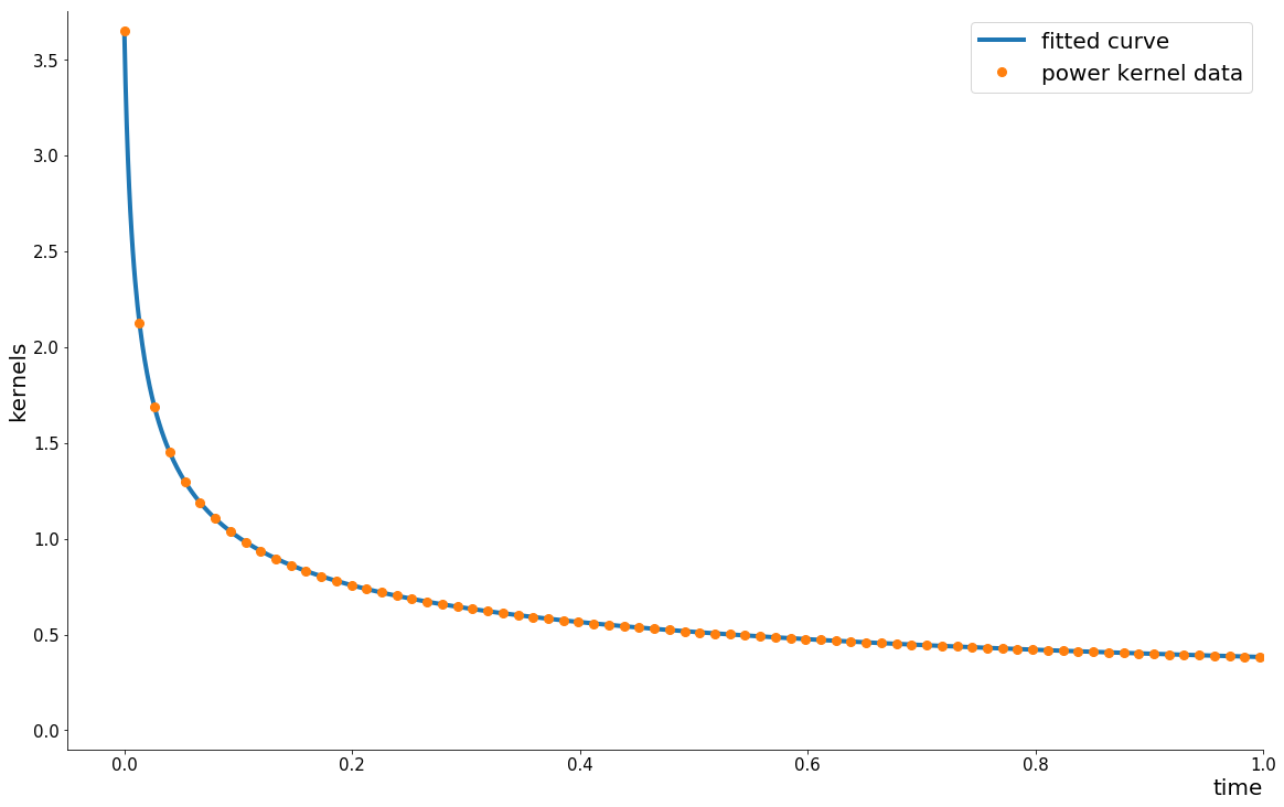
Figure 1: The power kernel $K_{\text{pow}}$ in the rBergomi model and the exponential $K_{\text{exp}}$ in the 25-term aBergomi model when $T=1$ and $N=100$.

Figure 1 displays the power kernel $K_{\text{pow}}$ in the rBergomi model and the $K_{\text{exp}}$ in the 25-term aBergomi model when $T=1$ and $N=100$. This figure suggests that $K_{\text{exp}}$ is sufficiently accurate for nonlinear regression, with a Root-mean-square error (RMSE) of $1.25095\times 10^{-5}$.

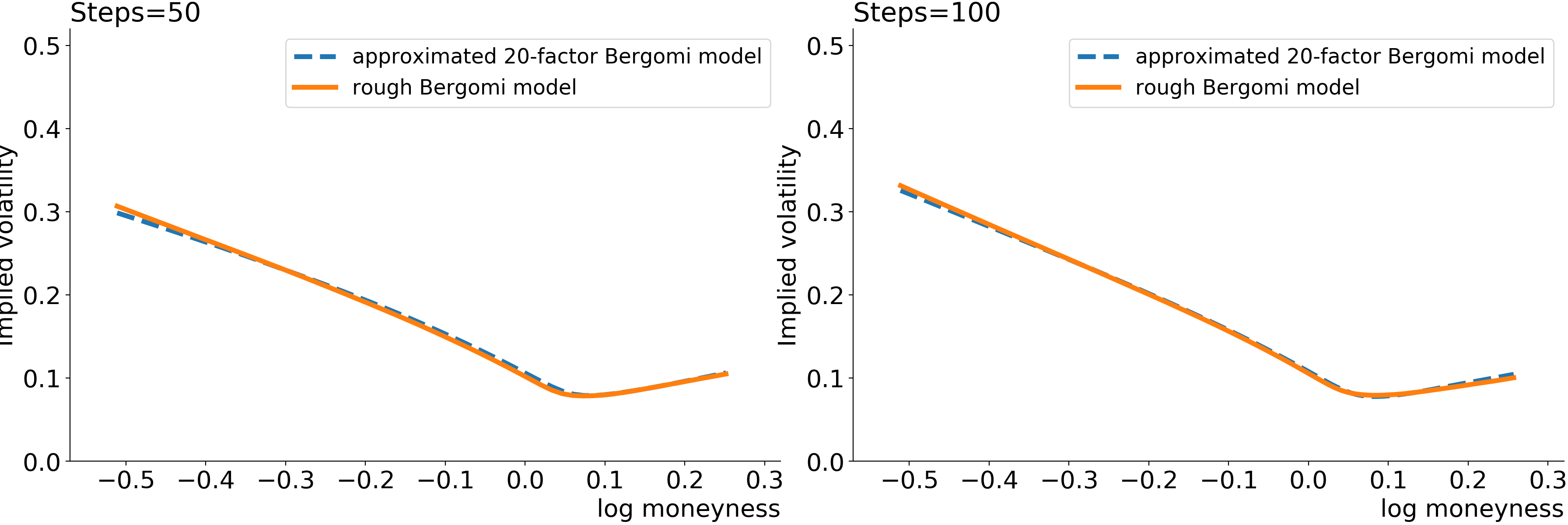
Figure 2: Volatility smiles for rBergomi and 25-term aBergomi models with $T=1$ simulated by $20000$ Monte Carlo paths.

The method for simulating the variance in the aBergomi model is described in Section 5.2, which leads directly to the volatility smiles in Figure 2 (see Algorithm 3). From Figure 2, we note that the at-the-money calibration is better with 50 time steps at the cost of a worse out-of-the-money calibration. Meanwhile, 100 time steps can approximate the rBergomi model visually well. However, we multiply the aBergomi smile by a constant for different time steps since the Riemann-sum scheme is able to capture the shape of the implied volatility smile, but not its level (see Bennedsen et al., 2017). To generate realistic implied volatility smiles, we determine the square of multiplication factors for different time steps in Table 2.

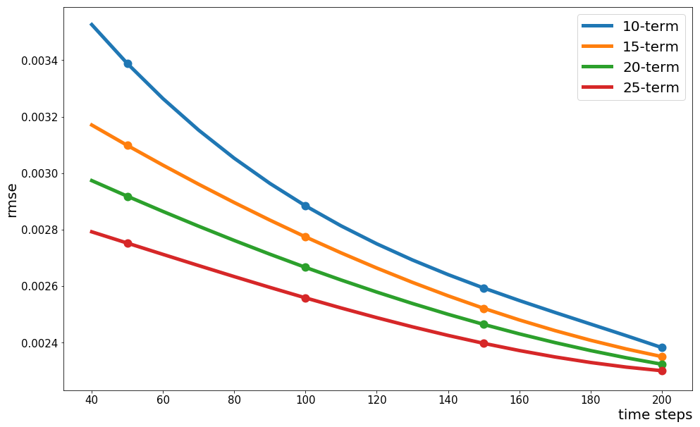
Figure 3: RMSE of the the implied volatility smiles of aBergomi model with three different number of terms (15, 20 and 25) at different number of time steps under 20000 Monte Carlo paths

Table 2: The square of multiplication factors for different steps

time steps	square of multiplication factors
50	0.750323909
100	0.550447453
150	0.485093611
200	0.450392126

$\triangleright$ Driftless Gaussian process $y_{s}=\sum_{i=1}^{n}\alpha_{i}e^{-\kappa_{i}(1-\theta)s}Y_{s}^{i}$

Set initial values $y_{s}=\text{zeros}(M,N)$, $Y_{0}^{i}=0$

while ($s=t_{1},t_{2},\cdots,t_{N}$ ) and ($i=1,2,\cdots,n$) do

       $Y_{s+\Delta t}\leftarrow Y_{s}^{i}+\kappa_{i}(1-\theta)Y_{s}^{i}\Delta t+\Delta W_{s}$

end while

$\triangleright$ Spot variance $V_{t}$

Set initial values $V_{t}=\xi_{0}$

while $t=t_{1},t_{2},\cdots,t_{N}$ do

      $V_{t}=\xi_{0}e^{\text{multiplication factor}\cdot\sqrt{\theta}y_{t}-\frac{\eta^{2}}{2}t^{2\alpha+1}}$

end while

$\triangleright$ Log-stock price $\log(S_{t})$

Set initial values $\log(S_{t})=0$

while $t=t_{1},t_{2},\cdots,t_{N}$ do

      $\log(S_{t+\Delta t})\leftarrow\log(S_{t})+\sqrt{V_{t}}\Delta W_{t}^{1}-\frac{1}{2}V_{t}\Delta t$

end while

Algorithm 3 n-term aBergomi model when $T=1$

Table 3: Runtime (in s) of the rBergomi model and the aBergomi model for different time steps with $T=1$ and 20000 Monte Carlo paths

Time steps	rBergomi	10-term aBergomi	15-term aBergomi	20-term aBergomi	25-term aBergomi
50	0.408105	0.099360	0.139226	0.172056	0.216408
100	0.500114	0.236882	0.313049	0.402372	0.454303
150	0.560219	0.365012	0.449856	0.558937	0.686911
200	0.586050	0.425685	0.590825	0.725772	0.872691

We compute the RMSE of the implied volatility approximation with different numbers of terms in the aBergomi model and different time steps in Figure 3 and compare the pricing speed in Table 3. The numerical results suggest that the RMSE of different term numbers reduces to the same low level as the number of time steps increases. Therefore, we may conclude that choosing the 25-term O-U process and 100 time steps can produce a good output, with reliable outcomes and fast calculation speed with 20000 Monte Carlo paths.

6 Conclusion

In this paper, we prove the power-law behavior of the ATM volatility skew as time to maturity goes to zero of the rBergomi model and we also propose an aBergomi model with finite terms to approximate the rBergomi model. The approximation enables the adoption of classical pricing methods while keeping the fractional feature of the model. When the terms number in the aBergomi model is large enough, we can prove its convergence to the rBergomi model. We not only give the theoretical proofs, but also give its numerical results. A hybrid scheme for the rBergomi model with the computational complexity $\mathcal{O}(N\log N)$ is developed for the aBergomi model. Numerically simulated results by the hybrid scheme demonstrate the accuracy and efficiency of the approximation.

The model parameters used in the numerical test are calibrated from the regression of the power-law kernel of the rBergomi model. Other efficient calibration methods are worth investigation for future research.

Appendix A Appendix

A.1 Proof of Theorem 7

In this subsection, we give the proof of the theoretical results in Theorem 7.

Proof.

Let $\left(p_{i}^{n}\right){}_{0\leq i\leq n}$ be auxiliary mean reversion speeds such that $p_{i-1}^{n}\leq x_{i}^{n}\leq p_{i}^{n}$ for $i\leq\{1,\cdots,n\}$ and $p_{0}^{n}=0$. Recall that $K(\tau)=\int_{0}^{\infty}e^{-x\tau}\mu(dx)$. We have

$$\|K^{n}-K\|_{2,T} =\left\|\sum_{i=1}^{n}\alpha_{i}^{n}e^{-x_{i}^{n}\tau}-\int_{0}^{\infty}e^{-x\tau}\mu\left(dx\right)\right\|_{2,T}$$ (28)

$$\leq\int_{0}^{\infty}\left\|e^{-x(\cdot)}\right\|_{2,T}\mu\left(dx\right)+\sum_{i=1}^{n}\left\|\alpha_{i}^{n}e^{-x_{i}^{n}(\cdot)}-\int_{p_{i-1}^{n}}^{p_{i}^{n}}e^{-x(\cdot)}\mu(dx)\right\|_{2,T}.$$

The first term on the RHS of the inequality (28) can be estimated as below:

$$\int_{p_{n}^{n}}^{\infty}\left\|e^{-x(\cdot)}\right\|_{2,T}\mu\left(dx\right)=\int_{p_{n}^{n}}^{\infty}\sqrt{\frac{1-e^{-2xT}}{2x}}\mu\left(dx\right)\leq\frac{\left(p_{n}^{n}\right){}^{-H}}{\sqrt{2}H\Gamma\left(\frac{1}{2}-H\right)}.$$

For the second term, applying a second-order Taylor expansion of the exponential function $e^{x}=1+x+\frac{x^{2}}{2}+\text{$\int_{0}^{x}\frac{(x-u)^{3}}{6}du$}$ for $t\in[0,T]$, choosing $\alpha_{i}^{n}=\int_{p_{i-1}^{n}}^{p_{i}^{n}}\mu\left(dx\right)$ and $x_{i}^{n}=\left(\frac{\int_{p_{i-1}^{n}}^{p_{i}^{n}}x^{4}\mu(dx)}{\int_{p_{i-1}^{n}}^{p_{i}^{n}}\mu(dx)}\right)^{\frac{1}{4}}$, we can obtain that

$$\begin{aligned} \left|\alpha_{i}^{n}e^{-x_{i}^{n}t}-\int_{p_{i-1}^{n}}^{p_{i}^{n}}e^{-xt}\mu\left(dx\right)\right|=&\left|\alpha_{i}^{n}\left(1+(-x_{i}^{n}t)+\frac{(-x_{i}^{n}t)^{2}}{2}\right)-\int_{p_{i-1}^{n}}^{p_{i}^{n}}\left(1+\left(-xt\right)+\frac{\left(-xt\right)^{2}}{2}\right)\mu\left(dx\right)\right|\\ &+\left|\alpha_{i}^{n}\left(\int_{0}^{x_{i}^{n}t}\frac{\left(x_{i}^{n}t-u\right)^{3}}{6}du\right)-\int_{p_{i-1}^{n}}^{p_{i}^{n}}\int_{0}^{xt}\frac{\left(xt-u\right)^{3}}{6}du\mu(dx)\right|\\ =&\int_{p_{i-1}^{n}}^{p_{i}^{n}}\left(xt-x_{i}^{n}t\right)+\frac{\left(-x_{i}^{n}t\right)^{2}-\left(-xt\right)^{2}}{2}\mu\left(dx\right)\\ \leq&\frac{t^{2}}{2}\int_{p_{i-1}^{n}}^{p_{i}^{n}}\left(x-x_{i}^{n}\right)^{2}\mu\left(dx\right)\end{aligned}$$

since

$$\int_{p_{i-1}^{n}}^{p_{i}^{n}}\left\{\int_{0}^{x_{i}^{n}t}\frac{(x_{i}^{n}t-u)^{3}}{6}du-\int_{0}^{xt}\frac{(xt-u)^{3}}{6}du\right\}\mu(dx)$$

$$= \int_{p_{i-1}^{n}}^{p_{i}^{n}}\left\{x_{i}^{n}t\int_{0}^{1}\frac{(x_{i}^{n}t-x_{i}^{n}ts)^{3}}{6}ds-xt\int_{0}^{1}\frac{(xt-xts)^{3}}{6}ds\right\}\mu(dx)\,\,\,,\,\,\,s=\frac{u}{xt}$$

$$= \int_{p_{i-1}^{n}}^{p_{i}^{n}}\left\{\left(x_{i}^{n}t\right)^{4}\int_{0}^{1}\frac{(1-s)^{3}}{6}ds-\left(xt\right)^{4}\int_{0}^{1}\frac{(1-s)^{3}}{6}ds\right\}\mu(dx)$$

$$= \left\{t^{4}\int_{0}^{1}\frac{(1-s)^{3}}{6}ds\right\}\int_{p_{i-1}^{n}}^{p_{i}^{n}}\left\{\left(x_{i}^{n}\right)^{4}-\left(x\right)^{4}\right\}\mu(dx)$$

$$= \left\{t^{4}\int_{0}^{1}\frac{(1-s)^{3}}{6}ds\right\}\int_{p_{i-1}^{n}}^{p_{i}^{n}}\left\{\left(\frac{\int_{p_{i-1}^{n}}^{p_{i}^{n}}x\mu\left(dx\right)}{\int_{p_{i-1}^{n}}^{p_{i}^{n}}\mu\left(dx\right)}\right)^{4}-\left(x\right)^{4}\right\}\mu(dx)$$

$$= 0.$$

Hence,

$$\sum_{i=1}^{n}\left\|\alpha_{i}^{n}e^{-x_{i}^{n}(\cdot)}-\int_{p_{i-1}^{n}}^{p_{i}^{n}}e^{-x(\cdot)}\mu(dx)\right\|_{2,T}\leq\frac{T^{\frac{5}{2}}}{2\sqrt{5}}\sum_{i=1}^{n}\int_{p_{i-1}^{n}}^{p_{i}^{n}}\left(x-x_{i}^{n}\right){}^{2}\mu(dx).$$

Thus, the convergence of $K^{n}$ depends on the weights $\alpha_{i}$ and mean reversions $x_{i}$. Let $p_{i}^{n}=i\pi_{n}$ for each $i\in\{1,\cdots,n\}$ and $\pi_{n}>0$. We have

$$\sum_{i=1}^{n}\int_{p_{i-1}^{n}}^{p_{i}^{n}}(x-x_{i}^{n})^{2}\mu(dx) \leq\pi_{n}^{2}\int_{0}^{p_{n}^{n}}\mu(dx)=\frac{\pi_{n}^{\frac{5}{2}-H}n^{\frac{1}{2}-H}}{\left(\frac{1}{2}-H\right)\Gamma\left(\frac{1}{2}-H\right)}$$

We can also proceed to get the explicit expressions of $\alpha_{i}^{n}$ and $x_{i}^{n}$ as follows:

$$\alpha_{i}^{n} =\frac{\left(i\pi_{n}\right)^{\frac{1}{2}-H}-\left[(i-1)\pi_{n}\right]^{\frac{1}{2}-H}}{\left(\frac{1}{2}-H\right)\Gamma\left(\frac{1}{2}-H\right)},\ x_{i}^{n}=\frac{1-2H}{3-2H}\cdot\frac{\left(i\pi_{n}\right)^{\frac{3}{2}-H}-\left[(i-1)\pi_{n}\right]^{\frac{3}{2}-H}}{\left(i\pi_{n}\right)^{\frac{1}{2}-H}-\left[(i-1)\pi_{n}\right]^{\frac{1}{2}-H}}.$$

Since $p_{n}^{n}=n\pi_{n}\rightarrow\infty$ , we have $\pi_{n}^{\frac{5}{2}-H}n^{\frac{1}{2}-H}\rightarrow 0$ as $n\rightarrow+\infty$ when $\pi_{n}<n^{-\frac{1}{6}}$ ,

$$\left\|K^{n}-K\right\|_{2,T} \leq \frac{1}{\sqrt{2}H\Gamma\left(\frac{1}{2}-H\right)}\left[\left(p_{n}^{n}\right)^{-H}+\frac{T^{\frac{5}{2}}H}{\sqrt{10}\left(\frac{1}{2}-H\right)}\left(p_{n}^{n}\right)^{\frac{1}{2}-H}\pi_{n}^{2}\right]$$ (29)

$$= \frac{1}{\sqrt{2}H\Gamma\left(\frac{1}{2}-H\right)}\left[n^{-H}\pi_{n}^{-H}+\frac{T^{\frac{5}{2}}H}{\sqrt{10}\left(\frac{1}{2}-H\right)}n^{\frac{1}{2}-H}\pi_{n}^{\frac{5}{2}-H}\right]$$

$$= ax^{-H}+bx^{\frac{5}{2}-H}$$

Let $x=\pi_{n}$, RHS $y=ax^{-H}+bx^{\frac{5}{2}-H}$ and $y^{{}^{\prime}}=-aHx^{-H-1}+b\left(\frac{5}{2}-H\right)x^{\frac{3}{2}-H}=0$, solving for $x$, we have $x^{\frac{2}{5}}=\frac{aH}{b\left(\frac{5}{2}-H\right)}$, where $a=n^{-H}$ and $b=\frac{T^{\frac{5}{2}}H}{\sqrt{10}\left(\frac{1}{2}-H\right)}n^{\frac{1}{2}-H}$

$$x = \pi_{n}=\left[\frac{n^{-H}H\sqrt{10}\left(\frac{1}{2}-H\right)}{T^{\frac{5}{2}}Hn^{\frac{1}{2}-H}\left(\frac{5}{2}-H\right)}\right]^{\frac{2}{5}}=\left[\frac{n^{-\frac{1}{2}}\sqrt{10}\left(\frac{1}{2}-H\right)}{T^{\frac{5}{2}}\left(\frac{5}{2}-H\right)}\right]^{\frac{2}{5}}=\frac{n^{-\frac{1}{5}}}{T}\left[\frac{\sqrt{10}\left(\frac{1}{2}-H\right)}{\left(\frac{5}{2}-H\right)}\right]^{\frac{2}{5}}$$

When $\pi_{n}=\frac{n^{-\frac{1}{5}}}{T}\left[\frac{\sqrt{10}\left(\frac{1}{2}-H\right)}{\left(\frac{5}{2}-H\right)}\right]^{\frac{2}{5}}$, the RHS of equation (29) attains its minimum and $\|K^{n}-K\|_{2,T}\leq Cn^{\frac{-4H}{5}}$ where $C=\frac{1}{\sqrt{2}H\Gamma\left(\frac{1}{2}-H\right)}T^{H}\left[\frac{\sqrt{10}\left(\frac{1}{2}-H\right)}{\frac{5}{2}-H}\right]^{-\frac{5}{2}H}\frac{\frac{5}{2}}{\frac{5}{2}-H}$ is a constant. ∎

References

- Abi Jaber and El Euch, (2019) Abi Jaber, E. and El Euch, O. (2019). Multifactor approximation of rough volatility models. SIAM Journal on Financial Mathematics, 10(2):309–349.
- Bayer et al., (2016) Bayer, C., Friz, P., and Gatheral, J. (2016). Pricing under rough volatility. Quantitative Finance, 16(6):887–904.
- Bayer et al., (2018) Bayer, C., Hammouda, C. B., and Tempone, R. (2018). Hierarchical adaptive sparse grids for option pricing under the rough Bergomi model. arXiv preprint arXiv:1812.08533.
- Bayer et al., (2019) Bayer, C., Horvath, B., Muguruza, A., Stemper, B., and Tomas, M. (2019). On deep calibration of (rough) stochastic volatility models. arXiv preprint arXiv:1908.08806.
- Bennedsen et al., (2017) Bennedsen, M., Lunde, A., and Pakkanen, M. S. (2017). Hybrid scheme for Brownian semistationary processes. Finance and Stochastics, 21(4):931–965.
- Bergomi, (2005) Bergomi, L. (2005). Smile dynamics II. Risk magazine, 18(10).
- Bergomi, (2009) Bergomi, L. (2009). Smile dynamics IV. Risk magazine, 22(12).
- Bergomi and Guyon, (2012) Bergomi, L. and Guyon, J. (2012). Stochastic volatility’s orderly smiles. Risk, 25(5):60.
- Carmona et al., (2000) Carmona, P., Coutin, L., and Montseny, G. (2000). Approximation of some Gaussian processes. Statistical inference for stochastic processes, 3(1-2):161–171.
- Forde and Zhang, (2017) Forde, M. and Zhang, H. (2017). Asymptotics for rough stochastic volatility models. SIAM Journal on Financial Mathematics, 8(1):114–145.
- Fukasawa, (2017) Fukasawa, M. (2017). Short-time at-the-money skew and rough fractional volatility. Quantitative Finance, 17(2):189–198.
- Gatheral et al., (2018) Gatheral, J., Jaisson, T., and Rosenbaum, M. (2018). Volatility is rough. Quantitative Finance, 18(6):933–949.
- Gatheral and Keller-Ressel, (2019) Gatheral, J. and Keller-Ressel, M. (2019). Affine forward variance models. Finance and Stochastics, pages 1–33.
- Harms and Stefanovits, (2019) Harms, P. and Stefanovits, D. (2019). Affine representations of fractional processes with applications in mathematical finance. Stochastic Processes and their Applications, 129(4):1185–1228.
- Jacquier et al., (2018) Jacquier, A., Martini, C., and Muguruza, A. (2018). On VIX futures in the rough Bergomi model. Quantitative Finance, 18(1):45–61.
- James et al., (2013) James, G., Witten, D., Hastie, T., and Tibshirani, R. (2013). An introduction to statistical learning, volume 112. Springer.
- Jusselin and Rosenbaum, (2018) Jusselin, P. and Rosenbaum, M. (2018). No-arbitrage implies power-law market impact and rough volatility. Available at SSRN 3180582.
- McCrickerd and Pakkanen, (2018) McCrickerd, R. and Pakkanen, M. S. (2018). Turbocharging Monte Carlo pricing for the rough Bergomi model. Quantitative Finance, 18(11):1877–1886.
- Muravlev, (2011) Muravlev, A. A. (2011). Representation of a fractional Brownian motion in terms of an infinite-dimensional Ornstein-Uhlenbeck process. Russian Mathematical Surveys, 66(2):439–441.