The Wright functions of the second kind
in Mathematical Physics

1. abstract

In this review paper we stress the importance of the higher transcendental Wright functions of the second kind in the framework of Mathematical Physics. We first start with the analytical properties of the classical Wright functions of which we distinguish two kinds. We then justify the relevance of the Wright functions of the second kind as fundamental solutions of the time-fractional diffusion-wave equations. Indeed, we think that this approach is the most accessible point of view.for describing Non-Gaussian stochastic processes and the transition from sub-diffusion processes to wave propagation. Through the sections of the text and suitable appendices we plan to address the reader in this pathway towards the applications of the Wright functions of the second kind.

Keywords: Fractional Calculus, Wright Functions, Green’s Functions, Diffusion-Wave Equation, Laplace Transform.
MSC: 26A33, 33E12, 34A08, 34C26.

2. Introduction

The special functions play a fundamental role in all fields of Applied Mathematics and Mathematical Physics because any analytical results are expressed in terms of some of these functions. Even if the topic of special functions can appear boring and their properties mainly treated in handbooks, we would promote the relevance of some of them not yet so well known. We devote our attention to the Wright functions, in particular with the class of the second kind. These functions, as we will see hereafter, are fundamental to deal with some non-standard deterministic and stochastic processes. Indeed the Gaussian function (known as the normal probability distribution) must be generalized in a suitable way in the framework of partial differential equations of non-integer order.
This work is organized as follows. In Section 2 we introduce the Wright functions, entire in the complex plane that we distinguish in two kinds in relation on the value-range of the two parameters on which they depend. In particular we devote our attention on two Wright functions of the second kind introduced by Mainardi with the term of auxiliary functions. One of them, known as M-Wright function generalizes the Gaussian function so it is expected to play a fundamental role in non-Gaussian stochastic processes.
Indeed In Section 3 we show how the Wright functions of the second kind are relevant in the analysis of time-fractional diffusion and diffusion-wave equations being related to their fundamental solutions. This analysis leads to generalize the known results r of the standard diffusion equation in the one-dimensional case, that is recalled in Appendix A by means of auxiliary functions as particular cases of the Wright functions of the second kind known as M-Wright or Mainardi functions. For readers’ convenience, in Appendix B we will also provide a introduction to the time-derivative of fractional order in the Caputo sense We remind that nowadays, as usual, by fractional order we mean a non-integer order,so that the term ”fractional” is a misnomer kept only for historical reasons.
In Section 4 we consider again the Mainsrdi auxiliary functions functions for their role in probability theory and in particular in the framework of Lévy stable distributions whose general theory is recalled in Appendix C.
In Section 5 we show how the auxiliary functions turn out to be included in a class that we denote the four sister functions. On their turn these four functions depending on a real parameter $\nu\in(0,1)$ are the natural generalization of the three sisters functions introduced in Appendix A devoted to the standard diffusion equation. The attribute of sisters was put by one of us (F. M.) because of their inter-relations, in his lecture notes on Mathematical Physics, so it has only a personal reason that we hope to be shared by the readers.
Finally, in Section 6, we provide some concluding remarks paying attention to work to be done in the next future.
We point out that we have equipped our theoretical analysis with several plots hoping they will be considered illuminating for the interested readers. We also note that we have limited our review to the simplest boundary values problems of equations in one space dimension referring the readers to suitable references for more general treatments in Section 3.1.

3. The Wright functions of the second kind and the Mainardi auxiliary functions

The classical Wright function, that we denote by $W_{\lambda,\mu}(z)$, is defined by the series representation convergent in the whole complex plane,

(1) $$W_{\lambda,\mu}(z):=\sum_{n=0}^{\infty}{\frac{z^{n}}{n!\Gamma(\lambda n+\mu)}},~{}~{}~{}\lambda>-1,~{}~{}~{}\mu\in\mathbb{C},$$

The integral representation reads as:

(2) $$W_{\lambda,\mu}(z)=\frac{1}{2\pi i}\int_{Ha_{-}}{e^{\sigma+z\sigma^{-\lambda}}\frac{d\sigma}{\sigma^{\mu}}},~{}~{}~{}\lambda>-1,~{}~{}~{}\mu\in\mathbb{C},$$

where $Ha_{-}$ denotes the Hankel path: this one is a loop which starts from $-\infty$ along the lower side of negative real axis, encircles with a small circle the axes origin and ends at $-\infty$ along the upper side of the negative real axis.
$W_{\lambda,\mu}(z)$ is then an entire function for all $\lambda\in(-1,+\infty)$. Originally Wright assumed $\lambda\geq 0$ in connection with his investigations on the asymptotic theory of partition [48, 49] and only in 1940 he considered $-1<\lambda<0$, [50]. We note that in the Vol 3, Chapter 18 of the handbook of the Bateman Project [10], presumably for a misprint, the parameter $\lambda$ is restricted to be non-negative, whereas the Wright functions remained practically ignored in other handbooks. In 1993 Mainardi, being aware only of the Bateman handbook, proved that the Wright function is entire also for $-1<\lambda<0$ in his approaches to the time fractional diffusion equation, that will be dealt in a next Section.
In view of the asymptotic representation in the complex domain and of the Laplace transform for positive argument $z=r>0$ ($r$ can be the time variable $t$ or the space variable $x$) the Wright functions are distinguished in first kind ($\lambda\geq 0$) and second kind ($-1<\lambda<0$) as outlined in the Appendix F of the book by Mainardi [35]. In particular, for the asymptotic behaviour, we refer the interested reader to the two papers by Wong and Zhao [46, 47], and to the surveys by Luchko and by Paris in the Handbook of Fractional Calculus and Applications, see respectively [25], [41], and references therein.
We note that the Wright functions are entire of order $1/(1+\lambda)$ hence only the first kind functions ($\lambda\geq 0$) are of exponential order whereas the second kind functions ($-1<\lambda<0$) are not of exponential order. The case $\lambda=0$ is trivial since $W_{0,\mu}(z)={{\rm e}^{z}}/{\Gamma(\mu)}.$ As a consequence of the distinction in the kinds, we must point out the different Laplace transforms proved e.g. in [15],[35], see also the recent survey on Wright functions by Luchko [25]. We have:
for the first kind, when $\lambda\geq 0$

(3) $$W_{\lambda,\mu}(\pm r)\,\div\,\frac{1}{s}\,E_{\lambda,\mu}\left(\pm\frac{1}{s}\right)\,;$$

for the second kind, when $-1<\lambda<0$ and putting for convenience $\nu=-\lambda$ so $0<\nu<1$

(4) $$W_{-\nu,\mu}(-r)\,\div\,E_{\nu,\mu+\nu}\left(-s\right)\,.$$

Above we have introduced the Mittag-Leffler function in two parameters $\alpha>0$, $\beta\in{\rm C\hskip-4.8pt\vrule height=6.0pt,width=0.1831pt\hskip 5.0pt}$ defined as its convergent series for all $z\in{\rm C\hskip-4.8pt\vrule height=6.0pt,width=0.1831pt\hskip 5.0pt}$

(5) $$E_{\alpha,\beta}(z):=\sum_{n=0}^{\infty}{\frac{z^{n}}{\Gamma(\alpha n+\beta)}}.$$

For more details on the special functions of the Mittag-leffler type we refer the interested readers to the treatise by Gorenflo et al [14], where in the forthcoming 2-nd edition also the Wright functions are treated in some detail.
In particular, two Wright functions of the second kind, originally introduced by Mainardi and named $F_{\nu}(z)$ and $M_{\nu}(z)$ ($0<\nu<1$), are called auxiliary functions in virtue of their role in the time fractional diffusion equations considered in the next section. These functions, $F_{\nu}(z)$ and $M_{\nu}(z)$, are indeed special cases of the Wright function of the second kind $W_{\lambda,\mu}(z)$ by setting, respectively, $\lambda=-\nu$ and $\mu=0$ or $\mu=1-\nu$. Hence we have:

(6) $$F_{\nu}(z):=W_{-\nu,0}(-z),~{}~{}~{}~{}0<\nu<1,$$

and

(7) $$M_{\nu}(z):=W_{-\nu,1-\nu}(-z),~{}~{}0<\nu<1,$$

Those functions are interrelated through the following relation:

(8) $$F_{\nu}(z)=\nu zM_{\nu}(z),$$

which reminds us the second relation in $(A.9)$, seen for the standard diffusion equation.
The series representations of the auxiliary functions are derived from those of $W_{\lambda,\mu}(z)$. Then:

(9) $$F_{\nu}(z):=\sum_{n=1}^{\infty}{\frac{(-z)^{n}}{n!\Gamma(-\nu n)}}=-\frac{1}{\pi}\sum_{n=1}^{\infty}{\frac{(-z)^{n}}{n!}\Gamma(\nu n+1)\sin{(\pi\nu n)}},$$

and

(10) $$M_{\nu}(z):=\sum_{n=0}^{\infty}{\frac{(-z)^{n}}{n!\Gamma[-\nu n+(1-\nu)]}}=\frac{1}{\pi}\sum_{n=1}^{\infty}{\frac{(-z)^{n-1}}{(n-1)!}\Gamma(\nu n)\sin{(\pi\nu n)}},$$

where it has been used in both cases the reflection formula for the Gamma function (Eq. 11) among the first and the second step of Eqs. (9) and (10),

(11) $$\Gamma(\zeta)\Gamma(1-\zeta)=\pi/\sin{\pi\zeta}.$$

Remark : In the present version we have corrected an error occurring in version V1 on the RHS of Eq. (9) referring to the $F_{\nu}$ function. Unfortunately this error was already present in the Appendix F of the first edition of the 2010 book by Mainardi [35].

Also the integral representations of the auxiliary functions are derived from those of $W_{\lambda,\mu}(z)$. Then:

(12) $$F_{\nu}(z):=\frac{1}{2\pi i}\int_{Ha_{-}}{e^{\sigma-z\sigma^{\nu}}d\sigma},~{}~{}~{}z\in\mathbb{C},~{}~{}~{}0<\nu<1$$

and

(13) $$M_{\nu}(z):=\frac{1}{2\pi i}\int_{Ha_{-}}{e^{\sigma-z\sigma^{\nu}}\frac{d\sigma}{\sigma^{1-\nu}}},~{}~{}~{}z\in\mathbb{C},~{}~{}~{}0<\nu<1$$

Explicit expressions of $F_{\nu}(z)$ and $M_{\nu}(z)$ in terms of known functions are expected for some particular values of $\nu$ as shown and recalled by Mainardi in the first 1990’s in a series of papers [29, 30, 31, 32], that is

(14) $$M_{1/2}(z)=\frac{1}{\sqrt{\pi}}e^{-z^{2}/4},$$

(15) $$M_{1/3}(z)=3^{2/3}\hbox{Ai}(z/3^{1/3}),.$$

Liemert and Klenie [21] have added the following expression for $\nu=2/3$

(16) $$M_{2/3}(z)=3^{-2/3}\left[3^{1/3}\,z\,\hbox{Ai}\left(z^{2}/3^{4/3}\right)-3\hbox{Ai}^{\prime}\left(z^{2}/3^{4/3}\right)\right]\,{\rm e}^{-2z^{3}/27},$$

where Ai and $\hbox{Ai}^{\prime}$ denote the Airy function and its first derivative. Furthermore they have suggested in the positive real field $\vbox{\hbox to8.9pt{I\hskip-2.1ptR\hfil}}^{+}$ the following remarkably integral representation

(17) $$M_{\nu}(x)=\frac{1}{\pi}\,\frac{x^{\nu/(1-\nu)}}{1-\nu}\,\int_{0}^{\pi}\!C_{\nu}(\phi)\,{\rm exp}\left(-C_{\nu}(\phi)\right)\,x^{1/(1-\nu)}\,d\phi,$$

where

(18) $$C_{\nu}(\phi)=\frac{\sin(1-\nu)}{\sin\phi}\,\left(\frac{\sin\nu\phi}{\sin\phi}\right)^{\nu/(1-\nu)}\,,$$

corresponding to equation (7) of the article written by Saa and Venegeroles [42] .
Let us point out the asymptotic behaviour of the function $M_{\nu}(x)$ as $x\to+\infty$. Choosing as a variable $x/\nu$ rather than $x$, the computation of the asymptotic representation by the saddle-point approximation carried out by Mainardi and Tomirotti yields, see [39] and [35],

(19) $$\!M_{\nu}(x/\nu)\sim a(\nu)\,x^{\displaystyle{(\nu-1/2)/(1-\nu)}}\,{\rm exp}\left[-b(\nu)\,x^{\displaystyle{1/(1-\nu)}}\right],$$

where

(20) $$a(\nu)=\frac{1}{\sqrt{2\pi\,(1-\nu)}}>0\,,\quad b(\nu)=\frac{1-\nu}{\nu}>0\,.$$

The above evaluation is consistent with the first term in the original asymptotic expansion by Wright in [49, 50] after having used the definition of .$M$-Wright function
Now we find it convenient to show the plots of the $M$-Wright functions on a space symmetric interval of IR in Figs 1, 2, corresponding to the cases $0\leq\nu\leq 1/2$ and $1/2\leq\nu\leq 1$, respectively. We recognize the non-negativity of the $M$-Wright function on IR for $1/2\leq\nu\leq 1$ consistently with the analysis on distribution of zeros and asymptotics of Wright functions carried out by Luchko, see [22], [25].

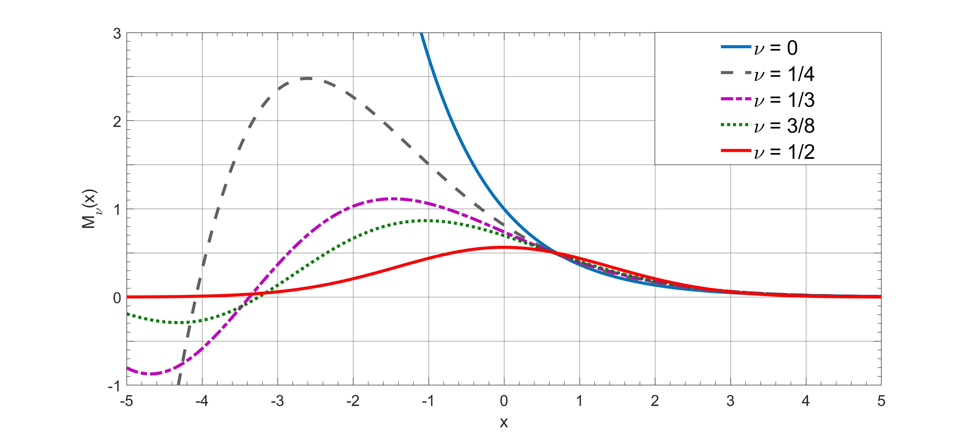
Figure 1. Plots of the $M$-Wright function as a function of the $x$ variable, for $0\leq\nu\leq 1/2$.

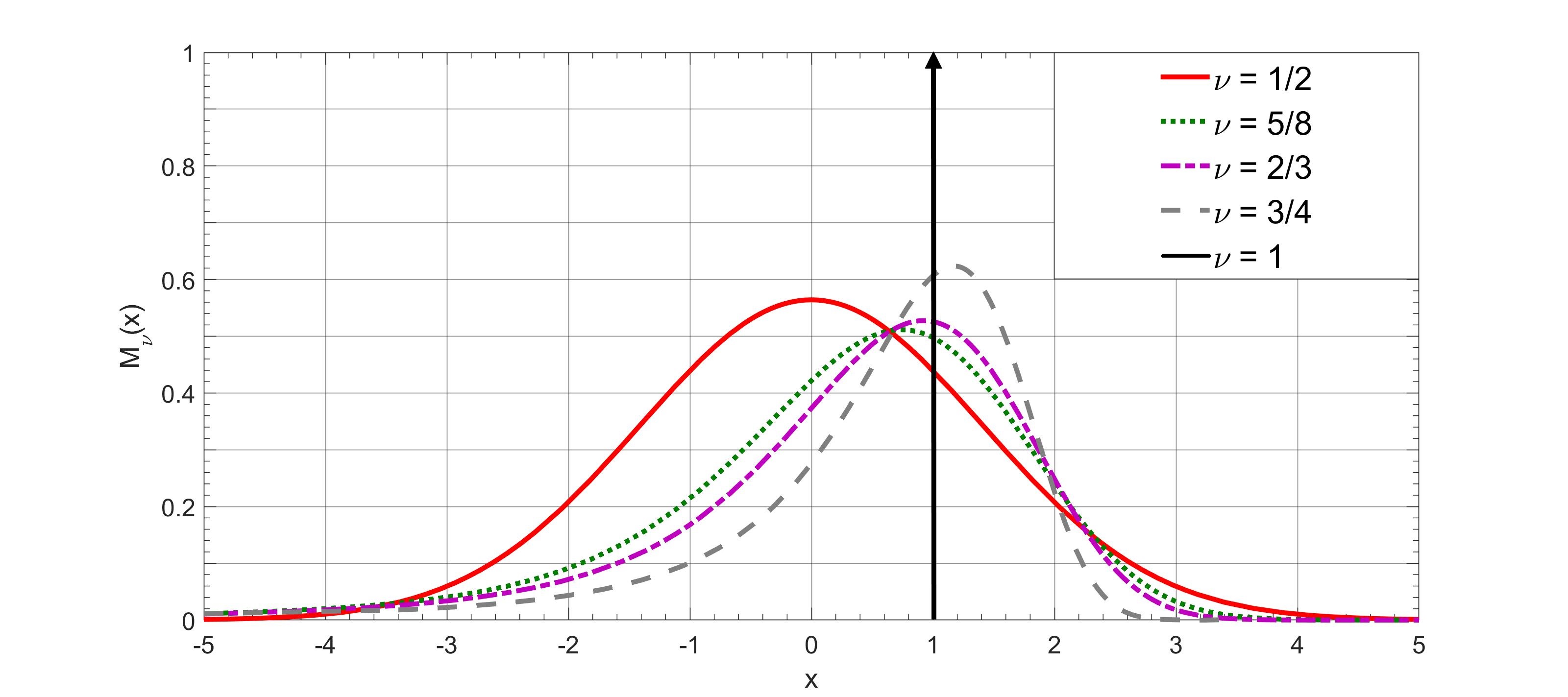
Figure 2. Plots of the $M$-Wright function as a function of the $x$ variable, for $1/2\leq\nu\leq 1$.

4. The Wright functions of the second kind and the time-fractional diffusion wave equation

As we will see the Wright functions of the second kind are relevant in the analysis of the Time-Fractional Diffusion-Wave Equation (TFDWE).
For this purpose we introduce now the TFDWE as a generalization of the standard diffusion equation and we see how the two Mainardi auxiliary functions come into play.
The TFDWE is so obtained from the standard diffusion equation (or the D’Alembert wave equation) by replacing the first-order (or the second-order) time derivative by a fractional derivative (of order $0<\beta\leq 2$) in the Caputo sense, obtaining the following Fractional PDE:

(21) $$\frac{\partial^{\beta}u}{\partial t^{\beta}}=D\frac{\partial^{2}u}{\partial x^{2}}~{}~{}~{}~{}~{}~{}~{}~{}0<\beta\leq 2,~{}~{}~{}~{}D>0,$$

where $D$ is a positive constant whose dimensions are $L^{2}T^{-\beta}$ and $u=u(x,t;\beta)$ is the field variable, which is assumed again to be a causal function of time. The Caputo fractional derivative is recalled in the Appendix B so that in explicit form the TFDWE (21) splits in the following integro-differential equations:

(22) $$\frac{1}{\Gamma(1-\beta)}\int_{0}^{t}{(t-\tau)^{-\beta}\biggl{(}\frac{\partial u}{\partial\tau}\biggl{)}d\tau}=D\,\frac{\partial^{2}u}{\partial x^{2}},~{}~{}~{}0<\beta\leq 1;$$

(23) $$\frac{1}{\Gamma(2-\beta)}\int_{0}^{t}{(t-\tau)^{1-\beta}\biggl{(}\frac{\partial^{2}u}{\partial\tau^{2}}\biggl{)}d\tau}=D\,\frac{\partial^{2}u}{\partial x^{2}},~{}~{}~{}1<\beta\leq 2.$$

In view of our analysis we find convenient to put:

(24) $$\nu=\frac{\beta}{2},~{}~{}~{}0<\nu\leq 1.$$

We can then formulate the basic problems for the Time Fractional Diffusion-Wave Equation using a correspondence with the two problems for the standard diffusion equation.
Denoting by $f(x)$ and $g(t)$ two given, sufficiently well-behaved functions, we define:
a) Cauchy problem

(25) $$\begin{cases}u(x,0^{+};\nu)=f(x),~{}~{}~{}~{}~{}~{}~{}~{}~{}~{}~{}~{}~{}~{}~{}~{}-\infty<x<+\infty;&\mbox{}\mbox{ }\\ u(\pm\infty,t;\nu)=0,~{}~{}~{}~{}~{}~{}~{}~{}~{}~{}~{}~{}~{}~{}~{}~{}~{}~{}~{}~{}~{}~{}t>0&\mbox{}\mbox{}\end{cases}$$

b) Signalling problem

(26) $$\begin{cases}u(x,0^{+};\nu)=0,~{}~{}~{}~{}~{}~{}~{}~{}~{}~{}~{}~{}~{}~{}~{}~{}~{}~{}~{}~{}~{}~{}~{}~{}0\leq x<+\infty;&\mbox{}\mbox{ }\\ u(0^{+},t;\nu)=g(t),~{}u(+\infty,t;\nu)=0,~{}~{}t>0&\mbox{}\mbox{}\end{cases}$$

If $1/2<\nu\leq 1$ corresponding to $1<\beta\leq 2$ we must consider also the initial value of the first time derivative of the field variable $u_{t}(x,0^{+};\nu)$, since in this case Eq. (21) turns out to be akin to the wave equation and consequently two linear independent solutions are to be determined. However, to ensure the continuous dependence of the solutions to our basic problems on the parameter $\nu$ in the transition from $\nu=(1/2)^{-}$ to $\nu=(1/2)^{+}$, we agree to assume $u_{t}(x,0^{+};\nu)=0$.

For the Cauchy and Signalling problems, following the approaches by Mainardi, see e.g. [29] and related papers, we introduce now the Green functions $\mathcal{G}_{c}(x,t;\nu)$ and $\mathcal{G}_{s}(x,t;\nu)$ that for both problems can be determined by the $LT$ technique, so extending the results known from the ordinary diffusion equation. We recall that the Green functions are also referred to as the fundamental solutions, corresponding respectively to $f(x)=\delta(x)$ and $g(t)=\delta(t)$ with $\delta(\cdot)$ is the Dirac delta generalized function
The expressions for the Laplace Transforms of the two Green’s functions are:

(27) $$\widetilde{\mathcal{G}}_{c}(x,s;\nu)=\frac{1}{2\sqrt{D}s^{1-\nu}}\,{\rm e}^{(-|x|/\sqrt{D})s^{\nu}}$$

and

(28) $$\widetilde{\mathcal{G}}_{s}(x,s;\nu)={\rm e}^{-(x/\sqrt{D})s^{\nu}}$$

Now we can easily recognize the following relation:

(29) $$\frac{d}{ds}\widetilde{\mathcal{G}}_{s}=-2\nu\,x\,\widetilde{\mathcal{G}}_{c},~{}~{}~{}x>0$$

which implies for the original Green functions the following reciprocity relation for $x>0$‘and $t>0$ and $0<\nu<1$:

(30) $$2\nu x\mathcal{G}_{c}(x,t;\nu)=t\mathcal{G}_{s}(x,t;\nu)=F_{\nu}(z)=\nu zM_{\nu}(z)\,,\quad z=\frac{x}{\sqrt{D}t^{\nu}}$$

where $z$ is the similarity variable and $F_{\nu}(z)$ and $M_{\nu}(z)$ are the Mainardi auxilary functions introduced in the previous section. Indeed Eq. (30) is the generalization of Eq. (A.8) that we have seen for the standard diffusion equation due to the introduction of the time fractional derivative of order $\nu$
Then, the two Green functions of the Cauchy and Signalling problems turn out to be expressed in terms of the two auxiliary functions as follows.
For the Cauchy problem we have

(31) $$\mathcal{G}_{C}(x,t;\nu)=\frac{t^{-\nu}}{2\sqrt{D}}\,M_{\nu}\left(\frac{|x|}{\sqrt{D}t^{\nu}}\right)\,,\quad-\infty<x<+\infty\,,\quad t\geq 0\,,$$

that generalizes Eq. (A.5).
For the Signalling problem we have:

(32) $$\mathcal{G}_{S}(x,t;\nu)=\frac{\nu xt^{-\nu-1}}{\sqrt{D}}\,M_{\nu}\left(\frac{x}{\sqrt{D}t^{\nu}}\right)\,,\quad x\geq 0,\quad t\geq 0\,,$$

that generalizes Eq. (A.7).

4.1. Complements to the time-fractional diffusion-wave equations

The boundary value problems dealt previously can be considered with a source data function $fx)$ and $g(t)$ different from the Dirac generalized functions, in particular with box-type functions as it has been carried out recently by us, see [8].

The TFDWE can be generalized in 2D and 3D space dimensions. so consequently the Wright functions play again a fundamental role. However, we prefer to refer the interested reader to the literature, in particular to the papers by Luchko and collaborators [22, 23, 24, 25], [27, 28], [1], by Hanyga [18] and to the recent analysis by Kemppainen [19]. All of them are originated in some way from the seminal paper by Schneider & Wyss [43]. In some of these papers the authors have considered also fractional differentiation both in time and in space, so that they have generalized to more than one dimension the former analysis by Mainardi, Luchko & Pagnini [37] on the space-time fractional diffusion-wave equations.

5. The $M-$Wright functions in probability theory and the stable distributions

We recognize that the Wright $M$-function with support in $\vbox{\hbox to8.9pt{I\hskip-2.1ptR\hfil}}^{+}$ can be interpreted as probability density function ($pdf$) because it is non negative and also it satisfies the normalization condition:

(33) $$\int_{0}^{\infty}{M_{\nu}(x)\,dx}=1\,.$$

We now provide more details on these densities in the framework of the theory of probability.
Fundamental quantities about the Wright $M-$function are the absolute moments of order $\delta>-1$ in $\mathbb{R}^{+}$, that are finite and turn out to be:

(34) $$\int_{0}^{\infty}{x^{\delta}\,M_{\nu}(x)\,dx}=\frac{\Gamma(\delta+1)}{\Gamma(\nu\delta+1)},~{}~{}~{}\delta>-1,~{}~{}~{}0\leq\nu<1.$$

The result is based on the integral representation of the $M-$Wright function:

(35) $$\begin{split}\int_{0}^{\infty}{x^{\delta}M_{\nu}(x)dx}&=\int_{0}^{\infty}{x^{\delta}\Biggl{[}\frac{1}{2\pi i}\int_{Ha_{-}}{e^{\sigma-x\sigma^{\nu}}\frac{d\sigma}{\sigma^{1-\nu}}}\Biggl{]}dx}\\ &=\frac{1}{2\pi i}\int_{Ha_{-}}{e^{\sigma}\Biggl{[}\int_{0}^{\infty}{e^{-x\sigma^{\nu}}x^{\delta}dx}\Biggl{]}\frac{d\sigma}{\sigma^{1-\nu}}}\\ &=\frac{\Gamma(\delta+1)}{2\pi i}\int_{Ha_{-}}{\frac{e^{\sigma}}{\sigma^{\nu\delta+1}}d\sigma}=\frac{\Gamma(\delta+1)}{\Gamma(\nu\delta+1)}\end{split}$$

The exchange between two integrals and the following identity contributed to the final result for Eq. (35):

(36) $$\int_{0}^{\infty}{{\rm e}^{-x\sigma^{\nu}}x^{\delta}dx}=\frac{\Gamma(\delta+1)}{(\sigma^{\nu})^{\delta+1}}.$$

In particular, for $\delta=n\in{\rm I\hskip-2.0ptN}$, the above formula provides the moments of integer order. Indeed recalling the Mittag-Leffler function introduced in Eq. (5) with $\alpha=\nu$ and $\beta=1$:

(37) $$E_{\nu}(z):=\sum_{n=0}^{\infty}{\frac{z^{n}}{\Gamma(\nu n+1)}},~{}~{}~{}\nu>0,~{}~{}~{}z\in\mathbb{C},$$

the moments of integer order can also be computed from the Laplace transform pair

(38) $$M_{\nu}(x)\div E_{\nu}(s)\,,$$

proved in the Appendix F of [35] as follows:

(39) $$\int_{0}^{+\infty}\!\!\!x^{\,n}\,M_{\nu}(x)\,dx=\lim_{s\to 0}\,(-1)^{n}\,\frac{d^{n}}{ds^{n}}\,E_{\nu}(-s)=\frac{\Gamma(n+1)}{\Gamma(\nu n+1)}\,.$$

5.1. The auxiliary functions versus extremal stable densities

We find it worthwhile to recall the relations between the Mainardi auxilary functions and the extremal Lévy stable densities as proven in the 1997 paper by Mainardi and Tomirotti [40]. For readers’ convenience we refer to Appendix C for an essential account of the general Lévy stable distributions in probability. Indeed, from a comparison between the series expansions of stable densities in (C.8)-(C.9) and of the auxiliary functions in Eqs. (9) - (10), we recognize that the auxiliary functions are related to the extremal stable densities as follows

(40) $$L_{\alpha}^{-\alpha}(x)=\frac{1}{x}\,F_{\alpha}(x^{-\alpha})={\alpha\over x^{\alpha+1}}\,M_{\alpha}(x^{-\alpha})\,,\quad 0<\alpha<1\,,\quad x\geq 0\,,$$

(41) $$L_{\alpha}^{\alpha-2}(x)=\frac{1}{x}\,F_{1/\alpha}(x)={1\over\alpha}\,M_{1/\alpha}(x)\,,\quad 1<\alpha\leq 2\,,\quad-\infty<x<+\infty\,.$$

In the above equations, for $\alpha=1$, the skewness parameter turns out to be $\theta=-1$, so we get the singular limit

(42) $$L_{1}^{-1}(x)=M_{1}(x)=\delta(x-1)\,.$$

Hereafter we show the plots the extremal stable densities according to their expressions in terms of the $M$-Wright functions, see Eq. (40)., Eq. (41) for $\alpha=1/2$ and $\alpha=3/2$, respectively.

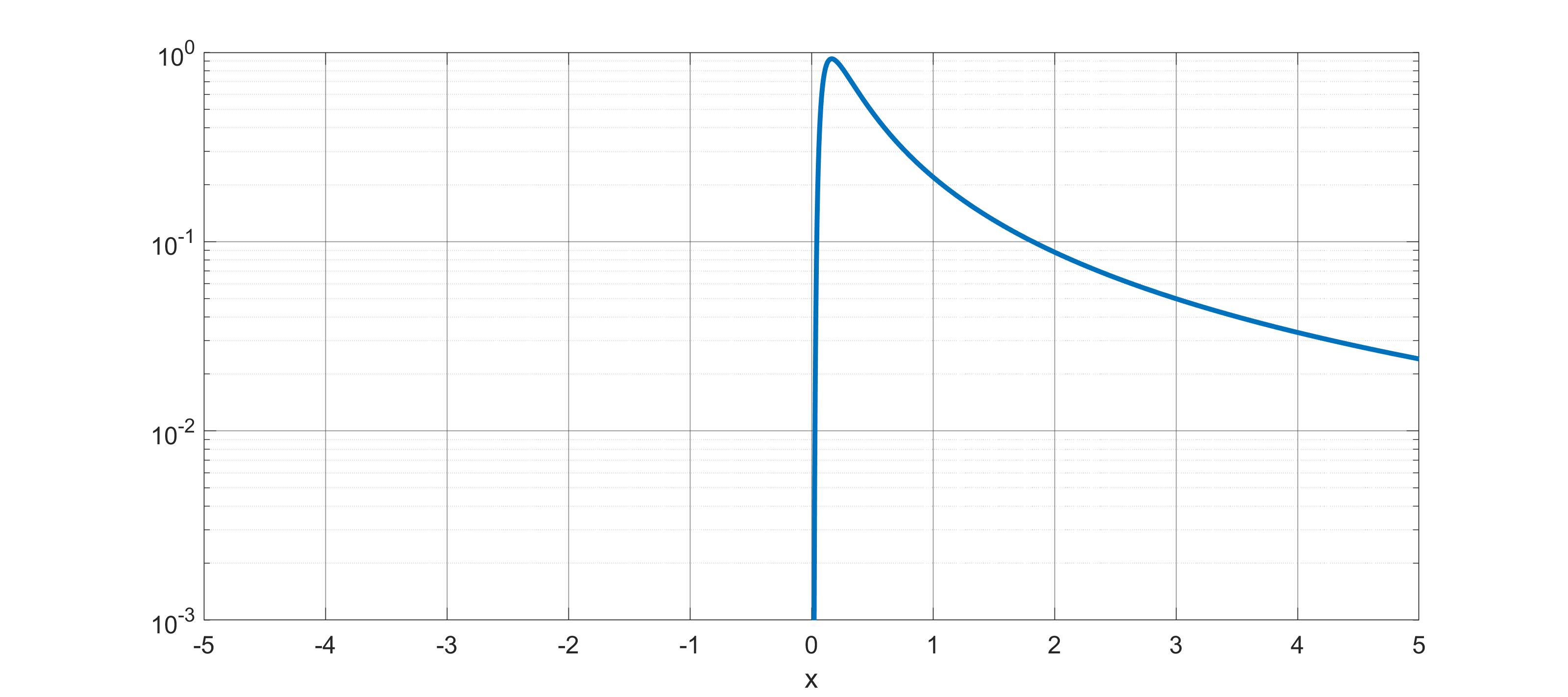
Figure 3. Plot of the unilateral extremal stable pdf for $\alpha=1/2$

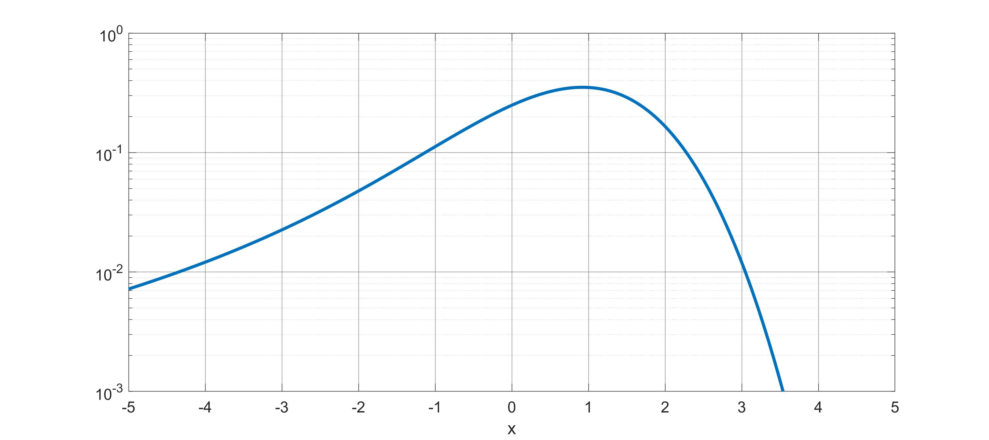
Figure 4. Plot of the bilateral extremal stable pdf for $\alpha=3/2$

We recognize that the above plots are consistent with the corresponding ones shown by Mainardi et al. [37] for the stable pdf’s derived as fundamental solutions of a suitable space-fractional diffusion equation.

5.2. The symmetric $M-$ Wright function

We easily recognize that extending the function $M_{\nu}(x)$ in a symmetric way to all of IR (that is putting $x=|x|$) and dividing by 2 we have a symmetric $pdf$ with support in all of IR .
As the parameter $\nu$ changes between 0 and 1, the pdf goes from the Laplace pdf to two half discrete delta pdfs passing for $\nu=1/2$ through the Gaussian pdf.
To develop a visual intuition, also in view of the subsequent applications, we show the plots of the symmetric $M-$Wright function on the real axis at $t=1$ for some rational values of the parameter $\nu\in[0,1]$

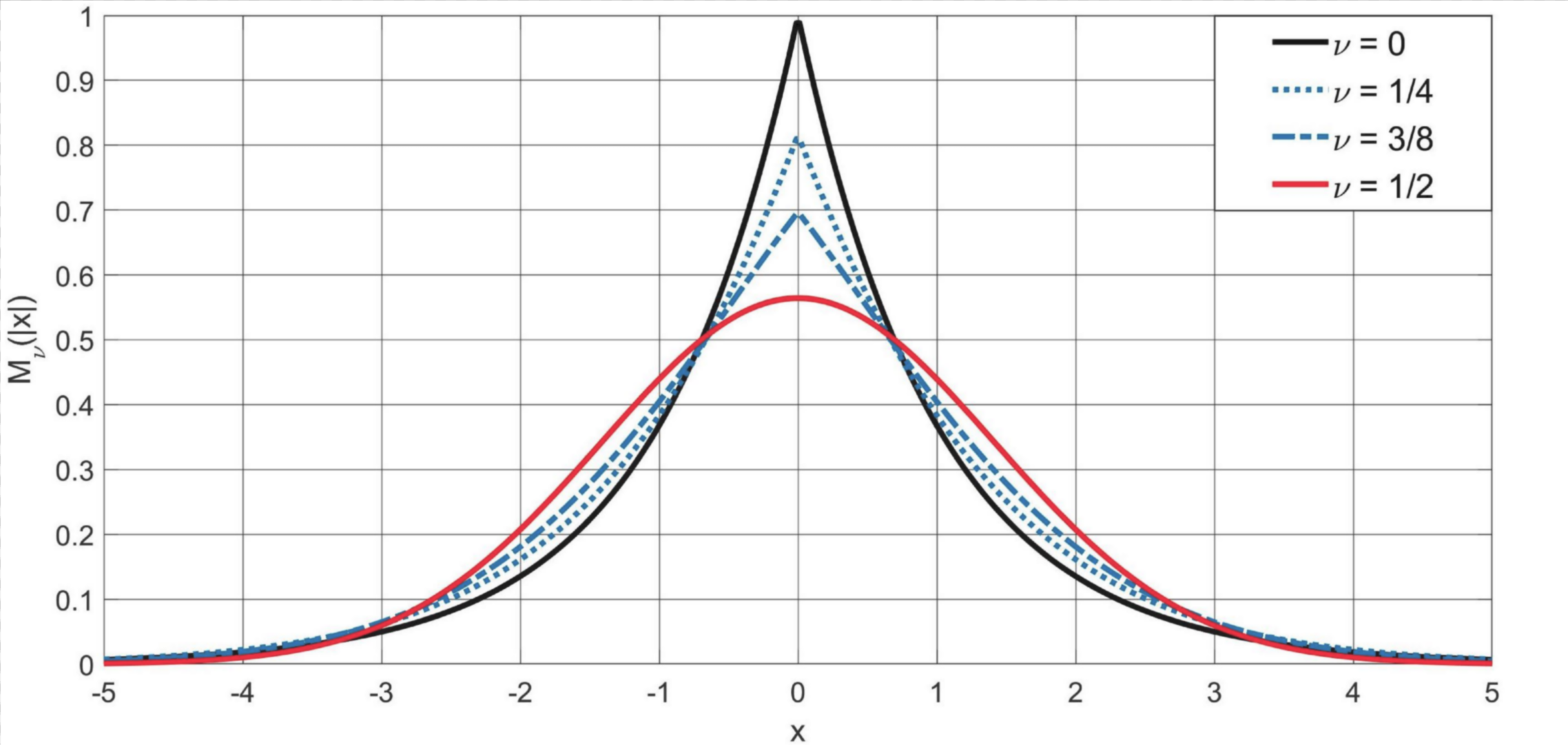
Figure 5. Plot of the symmetric $M-$Wright function $M_{\nu}(|x|)$ for $0\leq\nu\leq 1/2$. Note that the $M-$Wright function becomes a Gaussian density for $\nu=1/2$.

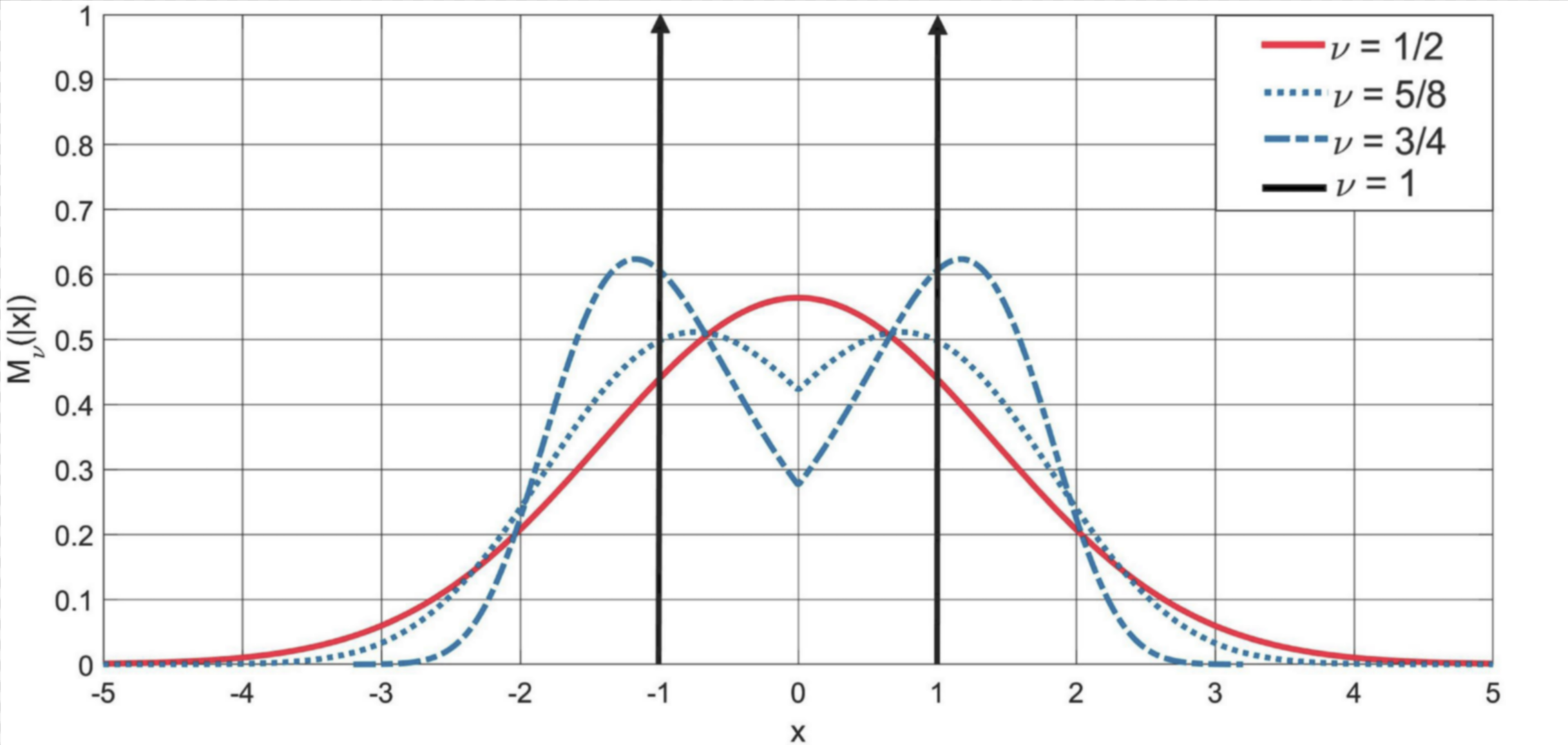
Figure 6. Plot of the symmetric $M-$Wright type function $M_{\nu}(|x|)|$ for $1/2\leq\nu\leq 1$. Note that the $M$Wright function becomes a a sum of two delta functions centered in $x=\pm 1$ for $\nu=1$.

The readers are invited to look the YouTube video by Consiglio whose title is “Simulation of the $M-$Wright function”, in which the author shows the evolution of this function as the parameter $\nu$ changes between 0 and 0.85 in a finite interval of IR centered in $x=0$.
Finally we compute the characteristic function for the symmetric $M-$Wright pdf. We get for $M_{\nu}(|x|$

(43) $$\begin{split}\mathcal{F}\Bigl{[}\frac{1}{2}M_{\nu}(|x|)\Bigl{]}&:=\frac{1}{2}\int_{-\infty}^{+\infty}{e^{+i\kappa x}M_{\nu}(|x|)dx}\\ &~{}=\int_{0}^{\infty}{\cos{(\kappa x)}M_{\nu}(x)dx}=E_{2\nu}(-\kappa^{2})\end{split}$$

Eq. 43 is obtained by developing in series the cosine function and using Eq. 35. In particular:

(44) $$\begin{split}\int_{0}^{\infty}{\cos{(\kappa x)}M_{\nu}(x)dx}&=\sum_{n=0}^{\infty}{(-1)^{n}\frac{\kappa^{2n}}{(2n)!}\int_{0}^{\infty}{x^{2n}}M_{\nu}(x)dx}\\ &=\sum_{n=0}^{\infty}{(-1)^{n}\frac{\kappa^{2n}}{\Gamma(2\nu n+1)}}=E_{2\nu}(-\kappa^{2})\end{split}$$

5.3. The Wright $\mathbb{M}$-function in two variables.

In view of time-fractional diffusion processes related to time-fractional diffusion equations it is worthwhile to introduce the function in two variables

(45) $$\mathbb{M}_{\nu}(x,t):=t^{-\nu}\,M_{\nu}(xt^{-\nu})\,,\quad 0<\nu<1\,,\quad x,t\in\vbox{\hbox to8.9pt{I\hskip-2.1ptR\hfil}}^{+}\,,$$

which defines a spatial probability density in $x$ evolving in time $t$ with self-similarity exponent $H=\nu$. Of course for $x\in\vbox{\hbox to8.9pt{I\hskip-2.1ptR\hfil}}$ we have to consider the symmetric version of the $M$-Wright function.
Hereafter we provide a list of the main properties of this function, which can be derived from the Laplace and Fourier transforms for the corresponding Wright $M$-function in one variable.
From Eqs. (39) and (43) we derive the Laplace transform of $\mathbb{M}_{\nu}(x,t)$ with respect to $t\in\vbox{\hbox to8.9pt{I\hskip-2.1ptR\hfil}}^{+}$,

(46) $${\mathcal{L}}\left\{\mathbb{M}_{\nu}(x,t);t\to s\right\}=s^{\nu-1}\,{\rm e}^{\displaystyle\,-xs^{\nu}}\,.$$

From Eq. (18) we derive the Laplace transform of $\mathbb{M}_{\nu}(x,t)$ with respect to $x\in\vbox{\hbox to8.9pt{I\hskip-2.1ptR\hfil}}^{+}$,

(47) $${\mathcal{L}}\left\{\mathbb{M}_{\nu}(x,t);x\to s\right\}=E_{\nu}\left(-st^{\nu}\right)\,.$$

From Eq. (55) we derive the Fourier transform of $\mathbb{M}_{\nu}(|x|,t)$ with respect to $x\in\vbox{\hbox to8.9pt{I\hskip-2.1ptR\hfil}}$,

(48) $${\mathcal{F}}\left\{\mathbb{M}_{\nu}(|x|,t);x\to\kappa\right\}=2E_{2\nu}\left(-\kappa^{2}t^{\nu}\right)\,.$$

Using the Mellin transforms, Mainardi et al. [38] derived the following interesting integral formula of composition,

(49) $$\mathbb{M}_{\nu}(x,t)=\int_{0}^{\infty}\mathbb{M}_{\lambda}(x,\tau)\,\mathbb{M}_{\mu}(\tau,t)\,d\tau\,,\quad\nu=\lambda\mu\,.$$

Special cases of the Wright $\mathbb{M}$-function are simply derived for $\nu=1/2$ and $\nu=1/3$ from the corresponding ones in the complex domain, see Eqs. (28)-(29). We devote particular attention to the case $\nu=1/2$ for which we get the Gaussian density in IR ,

(50) $$\mathbb{M}_{1/2}(|x|,t)=\frac{1}{2\sqrt{\pi}t^{1/2}}\,{\rm e}^{\displaystyle\,-x^{2}/(4t)}\,.$$

For the limiting case $\nu=1$ we obtain

(51) $$\mathbb{M}_{1}(|x|,t)=\frac{1}{2}\left[\delta(x-t)+\delta(x+t)\right]\,.$$

6. The four sisters

In this section we show how some Wright functions of the second kind can provide an interesting generalization of the three sisters discussed in Appendix A. The starting point is a (not well- known) paper published in 1970 by Stankovic [45], where (in our notation) the following Laplace transform pair is proved rigorously:

(52) $$t^{\mu-1}\,W_{{-\nu},\mu}(x,t)\div s^{-\mu}\,{\rm e}^{-xs^{\nu}}\,\quad 0<\nu<1\,,\quad\mu\geq 0\,,$$

where $x$ and $t$ are positive. We note that the Stankovic formula can be derived in a formal way by developing the exponential function in positive power of $s$ and inverting term by term as described in the Appendix F of the book by Mainardi [35].
We recognize that the Laplace Transforms of the Three Sisters functions $\widetilde{\phi}(x,s)$, $\widetilde{\psi}(x,s)$ and $\widetilde{\chi}(x,s)$ are particular cases of the Eq. (52) for $\nu=1/2$, that is of

(53) $$t^{\mu-1}\,W_{{-1/2},\mu}(x,t)\div s^{-\mu}\,{\rm e}^{-x\sqrt{s}},$$

according to the following scheme:

• $\widetilde{\phi}(x,s)$ with $\mu=1$,

• $\widetilde{\psi}(x,s)$ with $\mu=0$,

• $\widetilde{\chi}(x,s)$ with $\mu=1/2$.

If $\nu$ is no longer restricted to $\nu=1/2$ we define Four Sisters functions as follows

(54) $$\begin{split}\mu=0,~{}~{}~{}{\rm e}^{-xs^{\nu}}&\div t^{-1}W_{-\nu,0}(-xt^{-\nu}),\\ \mu=1-\nu,~{}~{}~{}\frac{{\rm e}^{-xs^{\nu}}}{s^{1-\nu}}&\div t^{-\nu}W_{-\nu,1-\nu}(-xt^{-\nu}),\\ \mu=\nu,~{}~{}~{}\frac{{\rm e}^{-xs^{\nu}}}{s^{\nu}}&\div t^{\nu-1}W_{-\nu,\nu}(-xt^{-\nu}),\\ \mu=1,~{}~{}~{}\frac{{\rm e}^{-xs^{\nu}}}{s}&\div W_{-\nu,1}(-xt^{-\nu}).\\ \end{split}$$

In the next figures we show some plots of these functions, both in the $t$ and in the $x$ domain for some values of $\nu$ ($\nu=1/4,1/2,3/4$).
Note that for $\nu=1/2$ we only find three functions, (the Three Sisters functions) of Appendix A

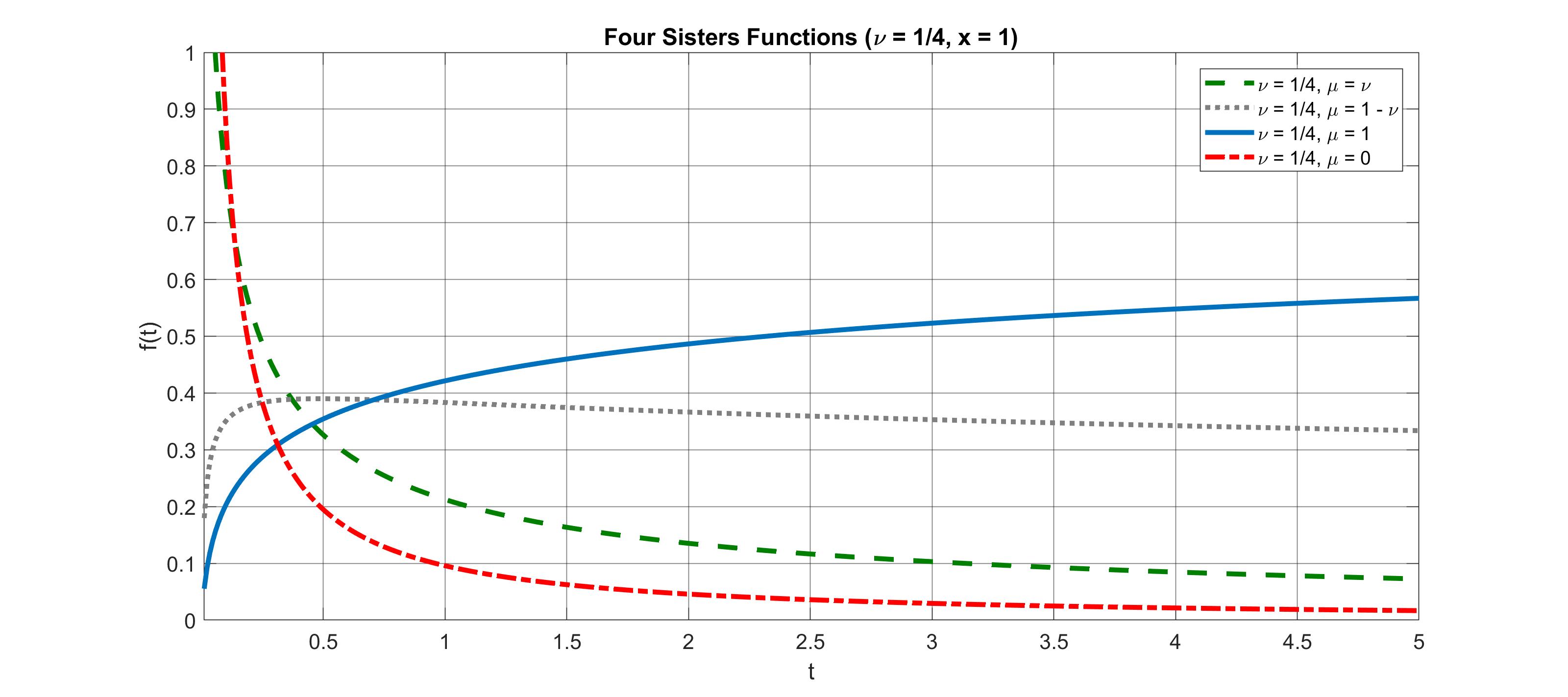
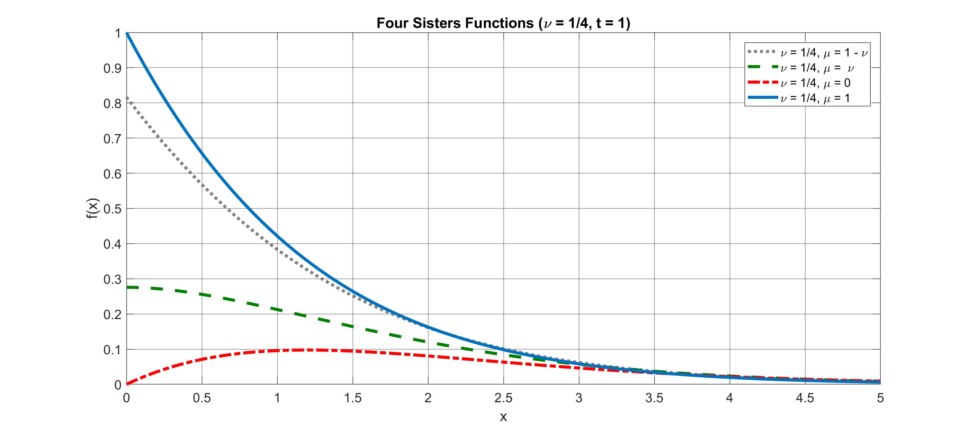
Figure 7. The four sisters functions in linear scale with $\nu=1/4$; top: versus $t$ ($x=1$), bottom: versus $x$ ($t=1$)

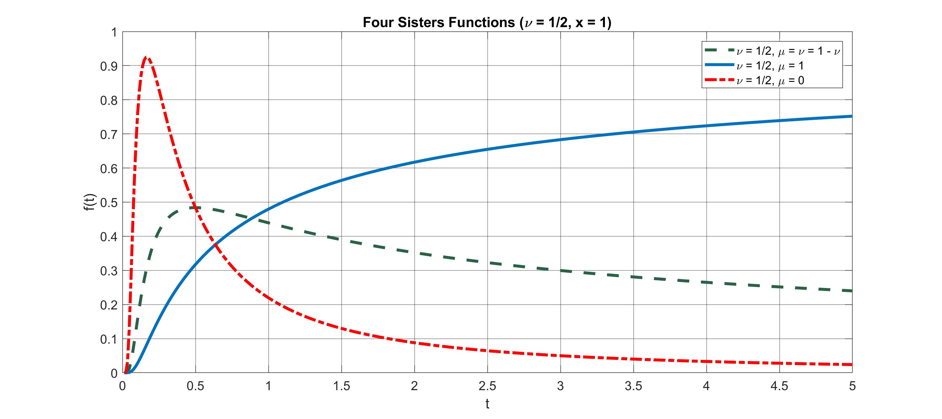
Figure 8. The three sisters functions in linear scale with $\nu=1/2$; top: versus $t$ ($x=1$), bottom: versus $x$ ($t=1$)

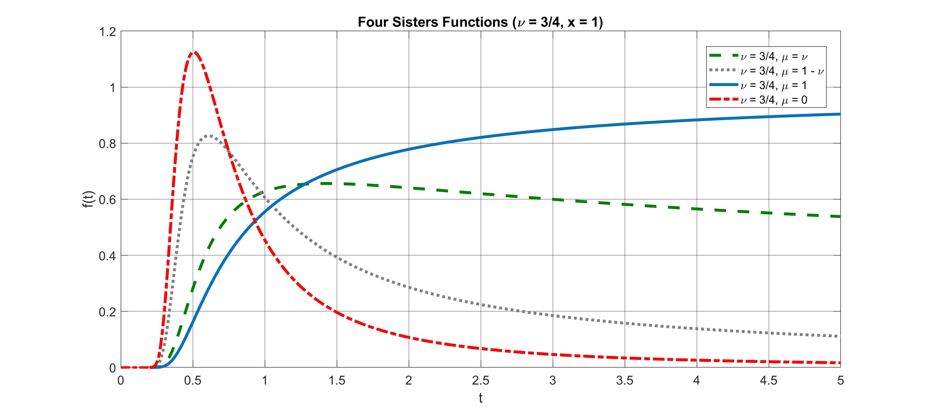
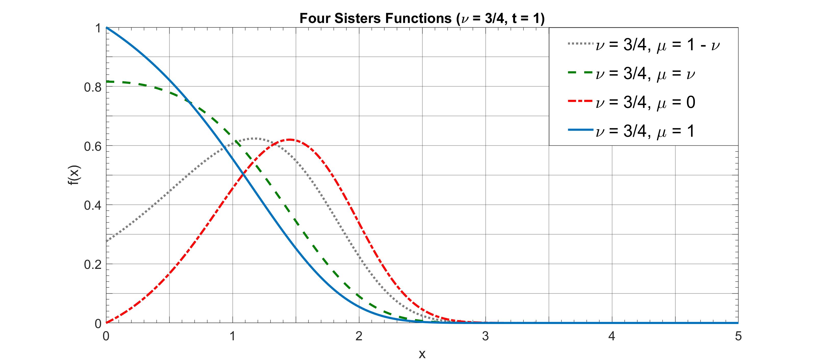
Figure 9. The four sisters functions in linear scale with $\nu=3/4$; top: versus $t$ ($x=1$), bottom: versus $x$ ($t=1$)

7. Conclusions

In our survey on the Wright functions we have distinguished two kinds, pointing out the particular class of the second kind. Indeed these functions have been shown to play key roles in several processes governed by non Gaussian processes, including sub-diffusion, transition to wave propagation, Lévy stable distributions.
Furthermore, we have devoted our attention to four functions of this class that we agree to called the Four Sisters functions.
All these items justify the relevance of the Wright functions of the second kind in Mathematical Physics.

Appendix A: The standard diffusion equation and the three sisters

In this Appendix let us recall the Diffusion Equation in the one-dimensional case

$(A.1)$ $$\frac{\partial u}{\partial t}=D\frac{\partial^{2}u}{\partial x^{2}}\,,$$

where the constant $D>0$ is the diffusion coefficient coefficient, whose dimensions are $L^{2}T^{-1}$ and $x$ , $t$ denote the space and time coordinates, respectively.
Two basic problems for Eq. ($(A.1)$) are the Cauchy and Signalling ones introduced hereafter In these problems some initial values and boundary conditions are set; specify the values attained by the field variable and/or by some of its derivatives on the boundary of the space-time domain is an essential step to guarantee the existence, the uniqueness and the determination of a solution of physical interest to the problem, not only for the Diffusion Equation.

Two data functions $f(x)$ and $g(t)$ are then introduced to write formally these conditions; some regularities are required to be satisfied by $f(x)$ and $g(t)$, and in particular $f(x)$ must admit the Fourier transform or the Fourier series expansion if the support is finite, while $h(t)$ must admit the Laplace Transform.
We also require without loss of generality that the field variable $u(x,t)$ is vanishing for $t<0$ for every $x$ in the spatial domain. Given these premises, we can specify the two aforementioned problems.
In the Cauchy problem the medium is supposed to be unlimited ($-\infty<x<+\infty$) and to be subjected at $t=0$ to a known disturbance provided by the data function $f(x)$. Formally:

$(A.2)$ $$\begin{cases}\lim_{t\rightarrow 0^{+}}{u(x,t)}=f(x),&-\infty<x<+\infty;\\ \lim_{x\rightarrow\pm\infty}{u(x,t)}=0,&~{}~{}~{}~{}~{}~{}~{}~{}~{}t>0.\end{cases}$$

This is a pure initial-value problem (IVP) as the values are specified along the boundary $t=0$.
In the Signalling problem the medium is supposed to be semi-infinite ($0\leq x<+\infty$) and initially undisturbed. At $x=0$ (the accessible end) and for $t>0$ the medium is then subjected to a known disturbance provided by the causal function $g(t)$. Formally:

$(A.3)$ $$\begin{cases}\lim_{t\rightarrow 0^{+}}{u(x,t)}=0,&0\leq x<+\infty;\\ \lim_{x\rightarrow 0^{+}}{u(x,t)}=g(t),~{}\lim_{x\rightarrow+\infty}{u(x,t)}=0&~{}~{}~{}~{}~{}~{}~{}~{}~{}t>0.\end{cases}$$

This problem is referred to as an initial boundary value problem (IBVP) in the quadrant $\{x,t\}>0$.
For each problem the solutions turn out to be expressed by a proper convolution between the data functions and the Green functions $\mathcal{G}$, that are the fundamental solutions of the problems.
For the Cauchy problem we have:

$(A.4)$ $$u(x,t)=\int_{-\infty}^{+\infty}{\mathcal{G}_{C}(\xi,t)f(x-\xi)d\xi}=\mathcal{G}_{C}(x,t)\ast f(x)\,,$$

with

$(A.5)$ $$\mathcal{G}_{C}(x,t)=\frac{1}{2\sqrt{\pi Dt}}{\rm e}^{-x^{2}/(4Dt)}.$$

For the Signalling problem we have:

$(A.6)$ $$u(x,t)=\int_{0}^{t}{\mathcal{G}_{S}(x,\tau)g(t-\tau)d\tau}=\mathcal{G}_{S}(x,t)\ast g(t)\,,\quad-\infty<x<+\infty,\quad t\geq 0\,,$$

with

$(A.7)$ $$\mathcal{G}_{S}(x,t)=\frac{x}{2\sqrt{\pi Dt^{3}}}{\rm e}^{-x^{2}/(4Dt)}\,,\quad x\geq 0,\quad t\geq 0\,.$$

Following the lecture notes in Mathematical Physics by Mainardi [34], we note that the following relevant property is valid for $\{x,t\}>0$:

$(A.8)$ $$x\mathcal{G}_{C}(x,t)=t\mathcal{G}_{S}(x,t)=F(z)$$

where

$(A.9)$ $$z=\frac{x}{\sqrt{Dt}},~{}~{}~{}~{}F(z)=\frac{z}{2}M(z),~{}~{}~{}~{}M(z)=\frac{1}{\sqrt{\pi}}{\rm e}^{-z^{2}/4}.$$

According to Mainardi’ s notations, Eq. ($(A.8)$) is known as reciprocity relation, $F(z)$ and $M(z)$ are called auxiliary functions and $z$ is the similarity variable.
A particular case of the Signalling problem is obtained when $g(t)=H(t)$ (the Heaviside unit step function) and the solution $u(x,t)$ turns out to be expressed in terms of the complementary error function:

$(A.10)$ $$u(x,t)=\mathcal{H}_{S}(x,t)=\int_{0}^{t}{\mathcal{G}_{S}(x,\tau)d\tau}=\hbox{erfc}\Bigl{(}\frac{x}{2\sqrt{Dt}}\Bigr{)}\,,\quad x\geq 0,\quad t\geq 0\,.$$

As well known, the three above fundamental solutions can be obtained via the Fourier and Laplace transform methods. Introducing the parameter $a=|x|/\sqrt{D}$ the Laplace transforms of these functions turns out to be simply related in the Laplace domain $\mathrm{Re}(s)>0$, as follows

$(A.11)$ $$\phi(a,t):=\hbox{erfc}\Bigl{(}\frac{a}{2\sqrt{t}}\Bigr{)}\div\frac{e^{-as^{1/2}}}{s}:=\widetilde{\phi}(a,s),$$

$(A.12)$ $$\psi(a,t):=\frac{a}{2\sqrt{\pi}}t^{-3/2}e^{-a^{2}/(4t)}\div e^{-as^{1/2}}:=\widetilde{\psi}(a,s),$$

$(A.13)$ $$\chi(a,t):=\frac{1}{\sqrt{\pi}}t^{-1/2}e^{-a^{2}/(4t)}\div\frac{e^{-as^{1/2}}}{s^{1/2}}:=\widetilde{\chi}(a,s)$$

where the sign $\div$ is used for the juxtaposition of a function with its Laplace transform. We easily note that Eq. ($(A.11)$) is related to the Step-Response problem, Eq. ($(A.12)$) is related to the Signalling problem and Eq. ($(A.13)$) is related to the Cauchy problem. Following the lecture notes by Mainardi [34] we agree to call the above functions the three sisters functions for their role in the standard diffusion equation. They will be discussed with details hereafter.
Everything that we have said above will be found again as a special case of the Time Fractional Diffusion Equation where the time derivative of the first order is replaced by a suitable time derivative of non-integer order.
It is easy to demonstrate that each of them can be expressed as a function of one of the 2 others three sisters (table 1).

	$\widetilde{\phi}$	$\widetilde{\psi}$	$\widetilde{\chi}$
$\widetilde{\phi}$	$\dfrac{\textrm{e}^{-a\sqrt{s}}}{s}$	$\dfrac{\widetilde{\psi}}{s}$	$-\dfrac{1}{s}\dfrac{\partial\widetilde{\chi}}{\partial a}$
$\widetilde{\psi}$	$s\;\widetilde{\phi}$	$\textrm{e}^{-a\sqrt{s}}$	$-\dfrac{\partial\widetilde{\chi}}{\partial a}$
$\widetilde{\chi}$	$-\dfrac{\partial\widetilde{\phi}}{\partial a}$	$-\dfrac{2}{a}\dfrac{\partial\widetilde{\psi}}{\partial s}$	$\dfrac{\textrm{e}^{-a\sqrt{s}}}{\sqrt{s}}$

Table 1. Relations among the three sisters in the Laplace domain.

The three sisters in the $t$ domain may be all directly calculated by making use of the Bromwich formula taking account of the contribution of the branch cut of $\sqrt{s}$ and of the pole of $1/s$. Wee obtain:

$(A.11a)$ $$\widetilde{\phi}(a,s)\div\phi(a,t)=1-\dfrac{1}{\pi}\int_{0}^{\infty}\textrm{e}^{-rt}\sin(a\sqrt{r})\dfrac{\mathop{}\!\mathrm{d}r}{r}\,,$$

$(A.12a)$ $$\widetilde{\psi}(a,s)\div\psi(a,t)=\dfrac{1}{\pi}\int_{0}^{\infty}\textrm{e}^{-rt}\sin(a\sqrt{r})\mathop{}\!\mathrm{d}r\,,$$

$(A.13a)$ $$\widetilde{\chi}(a,s)\div\chi(a,t)=\dfrac{1}{\pi}\int_{0}^{\infty}\textrm{e}^{-rt}\cos(a\sqrt{r})\dfrac{\mathop{}\!\mathrm{d}r}{\sqrt{r}}\,.$$

Then, through the substitution $\rho=\sqrt{r}$, we arrive at the Gaussian integral and, consequently, we find the previous explicit expressions of the three sisters, that is:

$(A.11)$ $$\phi(a,t)=\textrm{erfc}(\dfrac{a}{2\sqrt{t}})=1-\dfrac{2}{\sqrt{\pi}}\int_{0}^{a/2\sqrt{t}}\textrm{e}^{-u^{2}}\mathop{}\!\mathrm{d}u\,,$$

$(A.12)$ $$\psi(a,t)=\dfrac{a}{2\sqrt{\pi}}\>t^{-3/2}\>\textrm{e}^{-a^{2}/4t}\,,$$

$(A.13)$ $$\chi(a,t)=\dfrac{1}{\sqrt{\pi}}\>t^{-1/2}\>\textrm{e}^{-a^{2}/4t}\;,$$

reminding the definition of the complementary error function.
Alternatively, we can compute the three sisters in $t$ domain by using the relations among the three sisters in the Laplace domain listed in table 1. But in this case one of the three sisters in $t$ domain must be already known. Assuming to know $\phi(a,t)$ from Eq. (A.11), we get:

- $\psi(a,t)$ from $\widetilde{\psi}(a,s)=s\>\widetilde{\phi}(a,s)$. Indeed, noting

$$s\;\widetilde{\phi}(a,s)\div\dfrac{\partial}{\partial t}\>\phi(a,t)$$

since $\phi(a,0^{+})=0$ we can obtain (A.12), namely

$$\psi(a,t)=\dfrac{a}{2\sqrt{\pi}}\>t^{-3/2}\;\textrm{e}^{-a^{2}/4t}\,;$$

- $\chi(a,t)$ from $\widetilde{\chi}(a,s)=-\dfrac{\partial}{\partial a}\widetilde{\phi}(a,s)$ where $a$ is seen as a parameter,. Indeed it immediately follows (A.13), namely

$$\chi(a,t)=-\dfrac{\partial}{\partial a}\;\phi(a,t)=\dfrac{1}{\sqrt{\pi}}\>t^{-1/2}\>\textrm{e}^{-a^{2}/4t}\,.$$

For more details we refer the reader again to [34].

Appendix B: Essentials of Fractional Calculus

Fractional calculus is the field of mathematical analysis which deals with the investigation and applications of integrals and derivatives of arbitrary order. The term fractional is a misnomer, but it is retained for historical reasons, following the prevailing use.

This appendix is based on the 1997 surveys by Gorenflo and Mainardi [16] and by Mainardi [33]. For more details on the classical treatment of fractional calculus the reader is referred to the nice and rigorous book by Diethelm [9] published in 2010 by Springer in the series Lecture Notes in Mathematics.

According to the Riemann-Liouville approach to fractional calculus, the notion of fractional integral of order $\alpha$ ($\alpha>0$) is a natural consequence of the well known formula (usually attributed to Cauchy), that reduces the calculation of the $n-$fold primitive of a function $f(t)$ to a single integral of convolution type. In our notation the Cauchy formula reads

$(B.1)$ $$J^{n}f(t):=f_{n}(t)=\frac{1}{(n-1)!}\,\int_{0}^{t}\!\!(t-\tau)^{n-1}\,f(\tau)\,d\tau\,,\quad t>0\,,\quad n\in{\rm I\hskip-2.0ptN}\,,$$

where ${\rm I\hskip-2.0ptN}$ is the set of positive integers. From this definition we note that $f_{n}(t)$ vanishes at $t=0$ with its derivatives of order $1,2,\dots,n-1\,.$ For convention we require that $f(t)$ and henceforth $f_{n}(t)$ be a causal function, i.e. identically vanishing for $t<0\,.$

In a natural way one is led to extend the above formula from positive integer values of the index to any positive real values by using the Gamma function. Indeed, noting that $(n-1)!=\Gamma(n)\,,$ and introducing the arbitrary positive real number $\alpha\,,$ one defines the  Fractional Integral of order $\alpha>0$ :

$(B.2)$ $$J^{\alpha}\,f(t):=\frac{1}{\Gamma(\alpha)}\,\int_{0}^{t}(t-\tau)^{\alpha-1}\,f(\tau)\,d\tau\,,\quad t>0\,,\quad\alpha\in\vbox{\hbox to8.9pt{I\hskip-2.1ptR\hfil}}^{+}\,,$$

where $\vbox{\hbox to8.9pt{I\hskip-2.1ptR\hfil}}^{+}$ is the set of positive real numbers. For complementation we define $J^{0}:=I\,$ (Identity operator), i.e. we mean $J^{0}\,f(t)=f(t)\,.$ Furthermore, by $J^{\alpha}f(0^{+})$ we mean the limit (if it exists) of $J^{\alpha}f(t)$ for $t\to 0^{+}\,;$ this limit may be infinite.

We note the semigroup property $J^{\alpha}J^{\beta}=J^{\alpha+\beta}\,,\;\alpha\,,\;\beta\geq 0\,,$ which implies the commutative property $J^{\beta}J^{\alpha}=J^{\alpha}J^{\beta}\,,$ and the effect of our operators $J^{\alpha}$ on the power functions

$(B.3)$ $$J^{\alpha}t^{\gamma}={\Gamma(\gamma+1)\over\Gamma(\gamma+1+\alpha)}\,t^{\gamma+\alpha}\,,\quad\alpha\geq 0\,,\quad\gamma>-1\,,\quad t>0\,.$$

These properties are of course a natural generalization of those known when the order is a positive integer.

Introducing the Laplace transform by the notation ${\mathcal{L}}\,\left\{f(t)\right\}:=\int_{0}^{\infty}\!\!{\rm e}^{-st}\,f(t)\,dt=\widetilde{f}(s)\,,\;s\in{\rm C\hskip-4.8pt\vrule height=6.0pt,width=0.1831pt\hskip 5.0pt}\,,$ and using the sign $\div$ to denote a Laplace transform pair, i.e. $f(t)\div\widetilde{f}(s)\,,$ we note the following rule for the Laplace transform of the fractional integral,

$(B.4)$ $$J^{\alpha}\,f(t)\div{\widetilde{f}(s)\over s^{\alpha}}\,,\quad\alpha\geq 0\,,$$

which is the generalization of the case with an $n$-fold repeated integral.

After the notion of fractional integral, that of fractional derivative of order $\alpha$ ($\alpha>0$) becomes a natural requirement and one is attempted to substitute $\alpha$ with $-\alpha$ in the above formulas. However, this generalization needs some care in order to guarantee the convergence of the integrals and preserve the well known properties of the ordinary derivative of integer order.

Denoting by $D^{n}\,$ with $n\in{\rm I\hskip-2.0ptN}\,,$ the operator of the derivative of order $n\,,$ we first note that $D^{n}\,J^{n}=I\,,\;J^{n}\,D^{n}\neq I\,,\quad n\in{\rm I\hskip-2.0ptN}\,,$ i.e. $D^{n}$ is left-inverse (and not right-inverse) to the corresponding integral operator $J^{n}\,.$ In fact we easily recognize from (B.1) that

$(B.5)$ $$J^{n}\,D^{n}\,f(t)=f(t)-\sum_{k=0}^{n-1}f^{(k)}(0^{+})\,{t^{k}\over k!}\,,\quad t>0\,.$$

As a consequence we expect that $D^{\alpha}$ is defined as left-inverse to $J^{\alpha}$. For this purpose, introducing the positive integer $m$ such that $m-1<\alpha\leq m\,,$ one defines the Fractional Derivative of order $\alpha>0$ as $\;D^{\alpha}\,f(t):=D^{m}\,J^{m-\alpha}\,f(t)\,,$ i.e.

$(B.6)$ $$\!\!\!D^{\alpha}\,f(t):=\left\{\begin{split}&{\displaystyle{d^{m}\over dt^{m}}}\left[{\displaystyle\frac{1}{\Gamma(m-\alpha)}\int_{0}^{t}{f(\tau)\over(t-\tau)^{\alpha+1-m}}\,d\tau}\right],\qquad m-1<\alpha<m,\\ &{\displaystyle{d^{m}\over dt^{m}}}f(t)\,,\qquad\alpha=m\,.\end{split}\right.$$

Defining for complementation $D^{0}=J^{0}=I\,,$ then we easily recognize that $D^{\alpha}\,J^{\alpha}=I\,,$ $\,\alpha\geq 0\,,$ and

$(B.7)$ $$D^{\alpha}\,t^{\gamma}={\Gamma(\gamma+1)\over\Gamma(\gamma+1-\alpha)}\,t^{\gamma-\alpha}\,,\quad\alpha\geq 0\,,\quad\gamma>-1\,,\quad t>0\,.$$

Of course, these properties are a natural generalization of those known when the order is a positive integer.

Note the remarkable fact that the fractional derivative $D^{\alpha}\,f$ is not zero for the constant function $f(t)\equiv 1$ if $\alpha\not\in{{\rm I\hskip-2.0ptN}}\,.$ In fact, (B.7) with $\gamma=0$ teaches us that

$(B.8)$ $$D^{\alpha}1={t^{-\alpha}\over\Gamma(1-\alpha)}\,,\quad\alpha\geq 0\,,\quad t>0\,.$$

This, of course, is $\equiv 0$ for $\alpha\in{{\rm I\hskip-2.0ptN}}$, due to the poles of the gamma function in the points $0,-1,-2,\dots$. We now observe that an alternative definition of fractional derivative was introduced by Caputo in 1967 [3] in a geophysical journal and in 1969 [4] in a book in Italian. Then the Caputo definition was adopted in 1971 by Caputo and Mainardi [5, 6] in the framework of the theory of Linear Viscoelasticity. Nowadays it is usually referred to as the Caputo fractional derivative and reads $\;D_{*}^{\alpha}\,f(t):=J^{m-\alpha}\,D^{m}\,f(t)$ with $m-1<\alpha\leq m\,,\;m\in{\rm I\hskip-2.0ptN}\,,$ i.e.

$(B.9)$ $$D_{*}^{\alpha}\,f(t):=\left\{\begin{split}&{\displaystyle\frac{1}{\Gamma(m-\alpha)}}\,{\displaystyle\int_{0}^{t}{\displaystyle{f^{(m)}(\tau)\over(t-\tau)^{\alpha+1-m}}}\,d\tau}\,,\qquad m-1<\alpha<m\,,\\ &{\displaystyle{d^{m}\over dt^{m}}}f(t)\,,\qquad\alpha=m\,.\end{split}\right.$$

We note that there are a number of discussions on the priority of this definition that surely was formerly considered by Liouville as sated by Butzer and Westphal [2]. However Liouville did not recognize the relevance of this representation derived by a trivial integration by part whereas Caputo, even if unaware of the Riemann-Liouville representation, promoted his definition in several papers over all for the applications where the Laplace transform plays a fundamental role. We agree to denote (B.9) as the Caputo fractional derivative to distinguish it from the standard Riemann-Liouville fractional derivative (B.6).
The Caputo definition (B.9) is of course more restrictive than the Riemann-Liouville definition (B.6), in that requires the absolute integrability of the derivative of order $m$. Whenever we use the operator $D_{*}^{\alpha}$ we (tacitly) assume that this condition is met. We easily recognize that in general

$(B.10)$ $$D^{\alpha}\,f(t):=D^{m}\,J^{m-\alpha}\,f(t)\neq J^{m-\alpha}\,D^{m}\,f(t):=D_{*}^{\alpha}\,f(t)\,,$$

unless the function $f(t)$ along with its first $m-1$ derivatives vanishes at $t=0^{+}$. In fact, assuming that the passage of the $m$-derivative under the integral is legitimate, one recognizes that, for $m-1<\alpha<m\,$ and $t>0\,,$

$(B.11)$ $$D^{\alpha}\,f(t)=D_{*}^{\alpha}\,f(t)+\sum_{k=0}^{m-1}{t^{k-\alpha}\over\Gamma(k-\alpha+1)}\,f^{(k)}(0^{+})\,,$$

and therefore, recalling the fractional derivative of the power functions (B.7),

$(B.12)$ $$D^{\alpha}\left(f(t)-\sum_{k=0}^{m-1}{t^{k}\over k!}\,f^{(k)}(0^{+})\right)=D_{*}^{\alpha}\,f(t)\,.$$

The alternative definition (B.9) for the fractional derivative thus incorporates the initial values of the function and of its integer derivatives of lower order. The subtraction of the Taylor polynomial of degree $m-1$ at $t=0^{+}$ from $f(t)$ means a sort of regularization of the Riemann-Liouville fractional derivative. In particular for $0<\alpha<1$ we get

$$D^{\alpha}\left(f(t)-f(0^{+})\right)=D_{*}^{\alpha}\,f(t)\,.$$

According to the Caputo definition, the relevant property for which the fractional derivative of a constant is still zero can be easily recognized, i.e.

$(B.13)$ $$D_{*}^{\alpha}1\equiv 0\,,\quad\alpha>0\,.$$

We now explore the most relevant differences between the two fractional derivatives (B.6) and (B.9). We observe, again by looking at (B.7), that $D^{\alpha}t^{\alpha-1}\equiv 0\,,\;\alpha>0\,,\;t>0\,.$ From above we thus recognize the following statements about functions which for $t>0\,$ admit the same fractional derivative of order $\alpha\,,$ with $m-1<\alpha\leq m\,,$ $\;m\in{\rm I\hskip-2.0ptN}\,,$

$(B.14)$ $$D^{\alpha}\,f(t)=D^{\alpha}\,g(t)\,\Longleftrightarrow\,f(t)=g(t)+\sum_{j=1}^{m}c_{j}\,t^{\alpha-j}\,,$$

$(B.15)$ $$D_{*}^{\alpha}\,f(t)=D_{*}^{\alpha}\,g(t)\,\Longleftrightarrow\,f(t)=g(t)+\sum_{j=1}^{m}c_{j}\,t^{m-j}\,.$$

In these formulas the coefficients $c_{j}$ are arbitrary constants.

For the two definitions we also note a difference with respect to the formal   limit as $\alpha\to{(m-1)}^{+}$. From (B.6) and (B.9) we obtain respectively,

$(B.16)$ $$\alpha\to(m-1)^{+}\,\Longrightarrow\,D^{\alpha}\,f(t)\to D^{m}\,J\,f(t)=D^{m-1}\,f(t)\,;$$

$(B.17)$ $$\alpha\to{(m-1)}^{+}\,\Longrightarrow\,D_{*}^{\alpha}\,f(t)\to J\,D^{m}\,f(t)=D^{m-1}\,f(t)-f^{(m-1)}(0^{+})\,.$$

We now consider the Laplace transform of the two fractional derivatives. For the standard fractional derivative $D^{\alpha}$ the Laplace transform, assumed to exist, requires the knowledge of the (bounded) initial values of the fractional integral $J^{m-\alpha}$ and of its integer derivatives of order $k=1,2,\dots,m-1\,.$ The corresponding rule reads, in our notation,

$(B.18)$ $$D^{\alpha}\,f(t)\div s^{\alpha}\,\widetilde{f}(s)-\sum_{k=0}^{m-1}D^{k}\,J^{(m-\alpha)}\,f(0^{+})\,s^{m-1-k}\,,\quad m-1<\alpha\leq m\,.$$

The Caputo fractional derivative appears more suitable to be treated by the Laplace transform technique in that it requires the knowledge of the (bounded) initial values of the function and of its integer derivatives of order $k=1,2,\dots,m-1\,,$ in analogy with the case when $\alpha=m\,.$ In fact, by using (B.4) and noting that

$(B.19)$ $$\!\!\!\!J^{\alpha}\,D_{*}^{\alpha}\,f(t)=J^{\alpha}\,J^{m-\alpha}\,D^{m}\,f(t)=J^{m}\,D^{m}\,f(t)=f(t)-\sum_{k=0}^{m-1}{f^{(k)}(0^{+})}{t^{k}\over k!}.$$

we easily prove the following rule for the Laplace transform,

$(B.20)$ $$D_{*}^{\alpha}\,f(t)\div s^{\alpha}\,\widetilde{f}(s)-\sum_{k=0}^{m-1}f^{(k)}(0^{+})\,s^{\alpha-1-k}\,,\quad m-1<\alpha\leq m\,.$$

Indeed, the result (B.20), first stated by Caputo by using the Fubini-Tonelli theorem, appears as the most ”natural” generalization of the corresponding result well known for $\alpha=m\,.$
In particular Gorenflo and Mainardi have pointed out the major utility of the Caputo fractional derivative in the treatment of differential equations of fractional order for physical applications. In fact, in physical problems, the initial conditions are usually expressed in terms of a given number of bounded values assumed by the field variable and its derivatives of integer order, no matter if the governing evolution equation may be a generic integro-differential equation and therefore, in particular, a fractional differential equation.

Appendix C: The Lévy stable distributions

We now introduce the so-called Lévy stable distributions.. The term stable has been assigned by the French mathematician Paul Lévy, who, in the tuenties of the last century, started a systematic research in order to generalize the celebrated Central Limit Theorem to probability distributions with infinite variance. For stable distributions we can assume the following Definition: If two independent real random variables with the same shape or type of distribution are combined linearly and the distribution of the resulting random variable has the same shape, the common distribution (or its type, more precisely) is said to be stable.

The restrictive condition of stability enabled Lévy (and then other authors) to derive the canonic form for the characteristic function of the densities of these distributions. Here we follow the parameterization by Feller [11, 12] revisited by Gorenflo & Mainardi in [17], see also [37]. Denoting by $L_{\alpha}^{\theta}(x)$ a generic stable density in IR , where $\alpha$ is the index of stability and and $\theta$ the asymmetry parameter, improperly called skewness, its characteristic function reads:

$(C.1)$ $${\displaystyle L_{\alpha}^{\theta}(x)}\div{\displaystyle\widehat{L}_{\alpha}^{\theta}(\kappa)}={\displaystyle{\rm exp}\left[-\psi_{\alpha}^{\theta}(\kappa)\right]}\,,\quad{\displaystyle\psi_{\alpha}^{\theta}(\kappa)}={\displaystyle|\kappa|^{\displaystyle\alpha}\,{\rm e}^{\displaystyle i(\hbox{sign}\,\kappa)\theta\pi/2}}\,,$$

$$0<\alpha\leq 2\,,\;|\theta|\leq\,\hbox{min}\,\{\alpha,2-\alpha\}\,.$$

We note that the allowed region for the parameters $\alpha$ and $\theta$ turns out to be a diamond in the plane $\{\alpha,\theta\}$ with vertices in the points $(0,0)\,,\,(1,1)\,,\,(1,-1)\,,\,(2,0)$, that we call the Feller-Takayasu diamond, see Figure 10. For values of $\theta$ on the border of the diamond (that is $\theta=\pm\alpha$ if $0<\alpha<1$, and $\theta=\pm(2-\alpha)$ if $1<\alpha<2$) we obtain the so-called extremal stable densities.

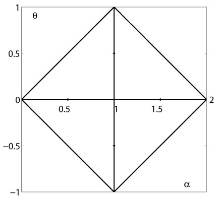
Figure 10. The Feller-Takayasu diamond for Lévy stable densities.

We note the symmetry relation $L_{\alpha}^{\theta}(-x)=L_{\alpha}^{-\theta}(x)$, so that a stable density with $\theta=0$ is symmetric.

Stable distributions have noteworthy properties of which the interested reader can be informed from the relevant existing literature. Here-after we recall some peculiar Properties:

- The class of stable distributions possesses its own domain of attraction, see e.g. [12].

- Any stable density is unimodal and indeed bell-shaped, i.e. its $n$-th derivative has exactly $n$ zeros in IR , see Gawronski [13], Simon [44] and Kwaśnicki [20].

- The stable distributions are self-similar and infinitely divisible.

These properties derive from the canonic form (C.1) through the scaling property of the Fourier transform.

Self-similarity means

$(C.2)$ $$L_{\alpha}^{\theta}(x,t)\div{\rm exp}\left[-t\psi_{\alpha}^{\theta}(\kappa)\right]\Longleftrightarrow L_{\alpha}^{\theta}(x,t)=t^{-1/\alpha}\,L_{\alpha}^{\theta}(x/t^{1/\alpha})]\,,$$

where $t$ is a positive parameter. If $t$ is time, then $L_{\alpha}^{\theta}(x,t)$ is a spatial density evolving on time with self-similarity.

Infinite divisibility means that for every positive integer $n$, the characteristic function can be expressed as the $n$th power of some characteristic function, so that any stable distribution can be expressed as the $n$-fold convolution of a stable distribution of the same type. Indeed, taking in (C.1) $\theta=0$, without loss of generality, we have

$(C.3)$ $${\rm e}^{-t|\kappa|^{\alpha}}=\left[{\rm e}^{-(t/n)|\kappa|^{\alpha}}\right]^{n}\Longleftrightarrow L_{\alpha}^{0}(x,t)=\left[L_{\alpha}^{0}(x,t/n)\right]^{*n}\,,$$

where

$$\left[L_{\alpha}^{0}(x,t/n)\right]^{*n}:=L_{\alpha}^{0}(x,t/n)*L_{\alpha}^{0}(x,t/n)*\dots*L_{\alpha}^{0}(x,t/n)$$

is the multiple Fourier convolution in IR with $n$ identical terms.

Only for a few particular cases, the inversion of the Fourier transform in (C.1) can be carried out using standard tables, and well-known probability distributions are obtained.

For $\alpha=2$ (so $\theta=0$), we recover the Gaussian pdf, that turns out to be the only stable density with finite variance, and more generally with finite moments of any order $\delta\geq 0$. In fact

$(C.4)$ $$L_{2}^{0}(x)=\frac{1}{2\sqrt{\pi}}{\rm e}^{\,\displaystyle-x^{2}/4}\,.$$

All the other stable densities have finite absolute moments of order $\delta\in[-1,\alpha)$ as we will later show.

For $\alpha=1$ and $|\theta|<1$, we get

$(C.5)$ $$L_{1}^{\theta}(x)=\frac{1}{\pi}\,{\cos(\theta\pi/2)\over[x+\sin(\theta\pi/2)]^{2}+[\cos(\theta\pi/2)]^{2}}\,,$$

which for $\theta=0$ includes the Cauchy-Lorentz pdf.

$(C.6)$ $$L_{1}^{0}(x)=\frac{1}{\pi}\frac{1}{1+x^{2}}\,.$$

In the limiting cases $\theta=\pm 1$ for $\alpha=1$ we obtain the singular Dirac pdf’s

$(C.7)$ $$L_{1}^{\pm 1}(x)=\delta(x\pm 1)\,.$$

In general, we must recall the power series expansions provided in [12]. We restrict our attention to $x>0$ since the evaluations for $x<0$ can be obtained using the symmetry relation. The convergent expansions of $L_{\alpha}^{\theta}(x)$ ($x>0$) turn out to be;
for $0<\alpha<1\,,\quad|\theta|\leq\alpha\,:$

$(C,8)$ $$L_{\alpha}^{\theta}(x)={1\over\pi\,x}\,\sum_{n=1}^{\infty}(-x^{-\alpha})^{n}\,{\Gamma(1+n\alpha)\over n!}\,\sin\left[{n\pi\over 2}(\theta-\alpha)\right]\,;$$

for $1<\alpha\leq 2\,,\quad|\theta|\leq 2-\alpha\,:$

$(C.9)$ $$L_{\alpha}^{\theta}(x)={1\over\pi\,x}\,\sum_{n=1}^{\infty}(-x)^{n}\,{\Gamma(1+n/\alpha)\over n!}\,\sin\left[{n\pi\over 2\alpha}(\theta-\alpha)\right]\,.$$

From the series in (C.8) and the symmetry relation we note that the extremal stable densities for $0<\alpha<1$ are unilateral, precisely vanishing for $x>0$ if $\theta=\alpha$, vanishing for $x<0$ if $\theta=-\alpha$. In particular the unilateral extremal densities $L_{\alpha}^{-\alpha}(x)$ with $0<\alpha<1$ have support in $\vbox{\hbox to8.9pt{I\hskip-2.1ptR\hfil}}^{+}$ and Laplace transform ${\rm exp}(-s^{\alpha})$. For $\alpha=1/2$ we obtain the so-called Lévy-Smirnov $pdf$:

$(C.10)$ $$L_{1/2}^{-1/2}(x)={\,x^{-3/2}\over 2\sqrt{\pi}}\,\,{\rm e}^{\displaystyle\,-1/(4x)}\,,\quad x\geq 0\,.$$

As a consequence of the convergence of the series in (C.8)-(C.9) and of the symmetry relation we recognize that the stable $pdf$’s with $1<\alpha\leq 2$ are entire functions, whereas with $0<\alpha<1$ have the form

$(C.11)$ $$L_{\alpha}^{\theta}(x)=\begin{cases}(1/x)\,\Phi_{1}(x^{-\alpha})&\hbox{for}\;x>0\,,\\ (1/|x|)\,\Phi_{2}(|x|^{-\alpha})&\hbox{for}\;x<0\,,\end{cases}$$

where $\Phi_{1}(z)$ and $\Phi_{2}(z)$ are distinct entire functions.The case $\alpha=1$ ($|\theta|<1$) must be considered in the limit for $\alpha\to 1$ of (C.8)-(C.9), because the corresponding series reduce to power series akin with geometric series in $1/x$ and $x$, respectively, with a finite radius of convergence. The corresponding stable $pdf$’s are no longer represented by entire functions, as can be noted directly from their explicit expressions (C.5)-(C.6).

We omit to provide the asymptotic representations of the stable densities referring the interested reader to Mainardi et al (2001) [37]. However, based on asymptotic representations, we can state as follows; for $0<\alpha<2$ the stable $pdf$’s exhibit fat tails in such a way that their absolute moment of order $\delta$ is finite only if $-1<\delta<\alpha$. More precisely, one can show that for non-Gaussian, not extremal, stable densities the asymptotic decay of the tails is

$(C.12)$ $$L_{\alpha}^{\theta}(x)=O\left(|x|^{-(\alpha+1)}\right)\,,\quad x\to\pm\infty\,.$$

For the extremal densities with $\alpha\neq 1$ this is valid only for one tail (as $|x|\to\infty$), the other (as $|x|\to\infty$) being of exponential order. For $1<\alpha<2$ the extremal $pdf$’s are two-sided and exhibit an exponential left tail (as $x\to-\infty)$ if $\theta=+(2-\alpha)\,,$ or an exponential right tail (as $x\to+\infty$) if $\theta=-(2-\alpha)\,.$ Consequently, the Gaussian $pdf$ is the unique stable density with finite variance. Furthermore, when $0<\alpha\leq 1$, the first absolute moment is infinite so we should use the median instead of the non-existent expected value in order to characterize the corresponding $pdf$.

Let us also recall a relevant identity between stable densities with index $\alpha$ and $1/\alpha$ (a sort of reciprocity relation) pointed out in [12], that is, assuming $x>0$,

$(C.13)$ $$\frac{1}{x^{\alpha+1}}\,L_{1/\alpha}^{\theta}(x^{-\alpha})=L_{\alpha}^{\theta^{*}}(x)\,,\;1/2\leq\alpha\leq 1\,,\;\theta^{*}=\alpha(\theta+1)-1\,.$$

The condition $1/2\leq\alpha\leq 1$ implies $1\leq 1/\alpha\leq 2$. A check shows that $\theta^{*}$ falls within the prescribed range $|\theta^{*}|\leq\alpha$ if $|\theta|\leq 2-1/\alpha$.
We leave as an exercise for the interested reader the verification of this reciprocity relation in the limiting cases $\alpha=1/2$ and $\alpha=1$.

References

- [1] Boyadjiev, L., Luchko, Yu., Mellin integral transform approach to analyze the multidimensional diffusion-wave equations. Chaos, Solitons & Fractals 2017, 102 127–134.
- [2] Butzer, P.L., Westphal, U. , Introduction to Fractional Calculus, in . Hilfer, H. (Editor), Fractional Calculus, Applications in Physics. World Scientific, Singapore 2000, pp. 1–85.
- [3] Caputo, M., Linear models of dissipation whose is almost frequency independent, Part II. Geophys. J. R. Astr. Soc. 1967, 13, 529–539. [Reprinted in Fract. Calc. Appl. Anal. 2008, 11 No 1, 4–14]
- [4] Caputo, M., Elasticità e Dissipazione Zanichelli, Bologna 1969. [in Italian]
- [5] Caputo, M., Mainardi, F., A new dissipation model based on memory mechanism. Pure and Appl. Geophys. (PAGEOPH) 1971,91, 134–147. [Reprinted in Fract. Calc. Appl. Anal.2007, 10 No 3, 309–324]
- [6] Caputo, M., Mainardi, F. Linear models of dissipation in anelastic solids. Riv. Nuovo Cimento (Ser. II) 1971, 1, 161–198.
- [7] Consiglio, A., Luchko., Yu.., Mainardi, F., Some notes on the Wright functions in probability theory. WSEAS Transactions on Mathematics2019, 18, 389–393.
- [8] Consiglio, A., Mainardi, F., On the Evolution of Fractional Diffusive Waves. Ricerche di Matematica, published on line 06 Dec 2019. DOI: 10.1007/s11587-019-00476-6 [E-print: arxiv.org/abs/1910.1259]
- [9] Diethelm, K., The Analysis of Fractional Differential Equations, An Application-Oriented Exposition Using Differential Operators of Caputo Type, Lecture Notes in Mathematics No 2004, Springer, Berlin 2010.
- [10] Erdélyi, A., Magnus, W., Oberhettinger, F and Tricomi, F., Higher Transcendental Functions, 3-rd Volume,. McGraw-Hill, New York 1955. [Bateman Project].
- [11] Feller, W., On a Generalization of Marcel Riesz’ Potentials and the Semi-Groups generated by Them. Meddelanden Lunds Universitets Matematiska Seminarium (Comm. Sém. Mathém. Université de Lund), Tome suppl. dédié à M. Riesz, Lund, 1952, pp. 73–81,
- [12] Feller, W., An Introduction to Probability Theory and its Applications. Wiley, New York, Vol. II 1971.
- [13] Gawronski, W., On the Bell-Shape of Stable Distributions. Annals of Probability 1984, 12, 230–242. .
- [14] Gorenflo, R., Kilbas, A.A., Mainardi, F., Rogosin, S., Mittag-Leffler Functions. Related Topics and Applications, Springer, Berlin 2014.
- [15] Gorenflo, R., Luchko, Yu., Mainardi, F., Analytical Properties and Applications of the Wright Function. Fract. Calc. Appl. Anal. 1999, 2, 383–414.
- [16] Gorenflo, R., Mainardi, F., Fractional Calculus: Integral and Differential Equations of Fractional Order, in: Carpinteri, A. and Mainardi, F. (Editors) Fractals and Fractional Calculus in Continuum Mechanics, Springer Verlag, Wien 1997, pp. 223–276. [E-print: http://arxiv.org/abs/0805.3823]
- [17] Gorenflo, R., Mainardi, F., Random Walk Models for Space-Fractional Diffusion Processes. Fract. Calc. Appl. Anal. 1998, 1, 167–191.
- [18] Hanyga, A., Multidimensional solutions of time-fractional diffusion-wave equations. R Soc Lond Proc Ser A Math Phys Eng Sci 2002. 458 (2020), 933–957.
- [19] Kemppainen, J., Positivity of the fundamental solution for fractional diffusion and wave wave equations. Published on line in Math Meth Appl Sci. 2019, 1–19. DOI: 10.1002/mma.5974 [ E-print arXiv:1906.04779]
- [20] Kwaśnicki, M., A new class of bell-shaped functions. Trans. Amer. Math. Soc 2020, in press. [E-print: arXiv:1710.11023, pp..24]
- [21] Liemert, A., Klenie, A., Fundamental Solution of the Tempered Fractional Diffusion Equation. J. Math. Phys 2015, 56, 113504.
- [22] Luchko, Yu, On the asymptotics of zeros of the Wright function. Zeitschrift für Analysis und ihre Anwendungen 2000, 19, 597–622.
- [23] Luchko, Yu., Multi-dimensional fractional wave equation and some properties of its fundamental solution. Commun. Appl. Ind. Math. 20146(1), 1–21. DOI: 10.1685/journal.caim.485
- [24] Luchko, Yu. On some new properties of the fundamental solution to the multi-dimensional space- and time-fractional diffusion-wave equation. Mathematics, 2017, 5 (4), 1–16..
- [25] Luchko, Yu., The Wright function and its applications, in A. Kochubei, Yu.Luchko (Eds.), Handbook of Fractional Calculus with Applications Volume 1: Basic Theory, pp. 241- 268, 2019. De Gruyter GmbH, 2019, Berlin/Boston, Series edited by J. A.Tenreiro Machado.
- [26] Luchko, Yu., Kiryakova, V. The Mellin integral transform in fractional calculus, Fract. Calc. Appl. Anal.2013, 16, 405–430.
- [27] Luchko, Yu., Mainardi, F., Cauchy and signaling problems for the time-fractional diffusion-wave equation ASME Journal of Vibration and Acoustics 2014, 136 No 5, , .050904/1–7. [E-print arXiv:1609.05443]
- [28] Luchko, Yu., Mainardi, F., Fractional diffusion-wave hhenomena, in V. Tarasov (Ed.), Handbook of Fractional Calculus with Applications Volume 5: Applications in physics, Part B, pp. 71–98, 2019. De Gruyter GmbH, 2019, Berlin/Boston, Series edited by J. A.Tenreiro Machado.
- [29] Mainardi, F.On the initial value problem for the fractional diffusion-wave equation, in: Rionero, S. and Ruggeri, T. (Editors), Waves and Stability in Continuous Media, World Scientific, Singapore 1994, pp. 246–251. [Proc. VII-th WASCOM, Int. Conf. ”Waves and Stability in Continuous Media”, Bologna, Italy, 4-7 October 1993]
- [30] Mainardi, F., The Time Fractional Diffusion-Wave-Equation. Radiophysics and Quantum Electronics 1995, No. 1-2, 20–36. [English translation from the Russian of Radiofisika]
- [31] Mainardi, F, The Fundamental Solutions for the Fractional Diffusion-Wave Equation. Applied Mathematics Letters,1996, 9 No 6, 23–28.
- [32] Mainardi, F., Fractional Relaxation-Oscillation and Fractional Diffusion-Wave Phenomena. Chaos, Solitons & Fractals 1996, 7, 1461–1477.
- [33] Mainardi, F., Fractional Calculus: Some Basic Problems in Continuum and Statistical Mechanics, in: Carpinteri, A. and Mainardi, F. (Editors) Fractals and Fractional Calculus in Continuum Mechanics. Springer Verlag, Wien, 1997, pp. 291–348. [E-print: arxiv.org/abs/1201.0863]
- [34] Mainardi, F., The Linear Diffusion Equation, Lecture Notes in Mathematical Physics, University of Bologna, Department of Physics, pp 19, 1996–2006. [Freely available since 2019 at Brown University at Series 4 of lectures http://www.dam.brown.edu/fractional_calculus/home.htm]
- [35] Mainardi, F., Fractional Calculus and Waves in Linear Viscoelasticity, Imperial College Press, London and World Scientific, Singapore, First Edition 2010.
- [36] Mainardi, F., Gorenflo, R., Time-Fractional Derivatives in Relaxation Processes: a Tutorial Survey, Fract. Calc. Appl. Anal. 2007, 10, 269–308. [E-print: arxiv.org/abs/0801.4914]
- [37] Mainardi, F., Luchko, Yu., Pagnini, G., The Fundamental Solution of the Space-Time Fractional Diffusion Equation. Fract. Calc. Appl. Anal. 2001, 4, 153–192. [E-print arxiv.org/abs/cond-mat/0702419]
- [38] Mainardi, F., Pagnini, G., Gorenflo, R. , Mellin Transform and Subordination Laws in Fractional Diffusion Processes. Fract. Calc. Appl. Anal. 2003, 6, No. 4, 441–459. [E-print:arxiv.org/abs/math/0702133]
- [39] Mainardi, F. and Tomirotti, M.,On a special function arising in the time fractional diffusion-wave equation. In P. Rusev, I. Dimovski and V. Kiryakova (Editors), Transform Methods and Special Functions, Sofia 1994, Science Culture Technology, Singapore (1995), pp. 171–183.
- [40] Mainardi, F. and Tomirotti, M.,Seismic Pulse Propagation with Constant and Stable Probability Distributions. Annali di Geofisica 1997, 40, 1311–1328. [E-print: arxiv.org/abs/1008.1341]
- [41] Paris, R.B., Asymptotics of the special functions of fractional calculus, in: A. Kochubei, Yu.Luchko (Eds.), Handbook of Fractional Calculus with Applications, Volume 1: Basic Theory, pp. 297-325, 2019. De Gruyter GmbH, 2019 Berlin/Boston, Series edited by J. A.Tenreiro Machado.
- [42] Saa, A., Venegeroles, R., Alternative numerical computation of one-sided Lévy and Mittag-Leffler distributions, Phys. Rev. E 2011, 84, 026702.
- [43] Schneider WR,Wyss W., Fractional diffusion and wave equations. J Math Phys 1989 30 (1), 134–144.
- [44] Simon, T., Positive Stable Densities and the Bell-Shape. Proc. Amer. Maqth. Soc. 2015, 143 No 2, 885–895.
- [45] Stankovi, B., On the function of E.M. Wright. Publ. de l’Institut Mathématique, Beograd, Nouvelle Sér. 1970, 10, 113–124.
- [46] Wong, R., Zhao, Y.-Q., Smoothing of Stokes’ discontinuity for the generalized Bessel function. Proc. R. Soc. London A 1999, 455, 1381–1400.
- [47] Wong, R., Zhao, Y.-Q. Smoothing of Stokes’ discontinuity for the generalized Bessel function II, Proc. R. Soc. London A (1999) 455, 3065–3084.
- [48] Wright, E.M., On the coefficients of power series having exponential singularities. Journal London Math. Soc. 1933, 8, 71–79.
- [49] Wright, E.M., The asymptotic expansion of the generalized Bessel function. Proc. London Math. Soc. (Ser. II) 1935, 38, 257–270.
- [50] Wright, E.M., The generalized Bessel function of order greater than one. Quart. J. Math., Oxford Ser. 1940,11, 36–48.