Piecewise Divergence-Free Nonconforming Virtual Elements for Stokes Problem in Any Dimensions

Abstract

Piecewise divergence-free nonconforming virtual elements are designed for Stokes problem in any dimensions. After introducing a local energy projector based on the Stokes problem and the stabilization, a divergence-free nonconforming virtual element method is proposed for Stokes problem. A detailed and rigorous error analysis is presented for the discrete method. An important property in the analysis is that the local energy projector commutes with the divergence operator. With the help of a divergence-free interpolation operator onto a generalized Raviart-Thomas element space, a pressure-robust nonconforming virtual element method is developed by simply modifying the right hand side of the previous discretization. A reduced virtual element method is also discussed. Numerical results are provided to verify the theoretical convergence.

76D07, 65N12, 65N22, 65N30

1 Introduction

In this paper, we shall construct piecewise divergence-free nonconforming virtual elements for Stokes problem in any dimensions. Assume that $\Omega\subset\mathbb{R}^{d}~{}(d\geq 2)$ is a bounded polytope. The Stokes problem is governed by

(1.1) $$\begin{cases}-\operatorname{div}(\nu\boldsymbol{\varepsilon}(\boldsymbol{u}))-\nabla p=\boldsymbol{f}&\textrm{ in }\Omega,\\ \qquad\qquad\qquad\operatorname{div}\boldsymbol{u}=0&\textrm{ in }\Omega,\\ \qquad\qquad\qquad\quad\;\;\boldsymbol{u}=\boldsymbol{0}&\textrm{ on }\partial\Omega,\end{cases}$$

where $\boldsymbol{u}$ is the velocity field, $p$ is the pressure, $\boldsymbol{\varepsilon}(\boldsymbol{u}):=(\nabla\boldsymbol{u}+(\nabla\boldsymbol{u})^{\intercal})/2$ is the symmetric gradient of $\boldsymbol{u}$, $\boldsymbol{f}\in\boldsymbol{L}^{2}(\Omega;\mathbb{R}^{d})$ is the external force field, and constant $\nu>0$ is the viscosity. The incompressibility constraint $\operatorname{div}\boldsymbol{u}=0$ in (1.1) describes the conservation of mass for the incompressible fluid.

Since the nonconforming $P_{1}$-$P_{0}$ element is a stable pair for the Stokes problem [19], as the generalization of the nonconforming $P_{1}$ element, it is spontaneous that the $H^{1}$-nonconforming virtual element in [5] is adopted to discretize the Stokes problem in [14, 26]. On the other hand, the incompressibility constraint is not satisfied exactly in general at the discrete level for the discrete methods in [14, 26], which is very important for the Navier-Stokes problem [24, 15]. To design the discrete method with the exact divergence-free discrete velocity, one idea is to combine the discontinuous Galerkin technique and the $H(\operatorname{div})$-conforming virtual elements, such as the divergence-free weak virtual element method [18]. The more compact idea in [7, 6, 1] is to construct divergence-free conforming virtual elements in two and three dimensions by defining the space of shape functions through the local Stokes problem with Dirichlet boundary condition. By enriching an $H(\operatorname{div})$-conforming virtual element with some divergence-free functions, a divergence-free nonconforming virtual element in two dimensions is advanced in [31], in which each element in the partition is required to be convex.

Following the ideas in [17, 23], we shall devise piecewise divergence-free $H^{1}$-nonconforming virtual elements in any dimensions based on the generalized Green’s identity for Stokes problem, which are also $H(\operatorname{div})$-nonconforming. The degrees of freedom of the proposed virtual elements for the velocity are same as those in [14], i.e. $d$ copies of the degrees of freedom of the $H^{1}$-nonconforming virtual elements in [5]. And the space of shape functions $\boldsymbol{V}_{k}(K)$ for the velocity is defined from the local Stokes problem with Neumann boundary condition, which is different from that in [7] due to the constraint on the boundary. Our virtual elements are locally divergence-free since $\operatorname{div}\boldsymbol{V}_{k}(K)=\mathbb{P}_{k-1}(K)$. The divergence-free velocity means the mass conservation. It is pointed out in [15] that many important conservation laws are lost with the loss of mass conservation, including energy, momentum, angular momentum. A common theme for all ‘enhanced-physics’ based schemes is that the more physics is built into the discretization, the more accurate and stable the discrete solutions are, especially over longer time intervals [15].

A novelty of this paper is to introduce a local energy projector $\boldsymbol{\Pi}_{k}^{K}:\boldsymbol{H}^{1}(K;\mathbb{R}^{d})\to\mathbb{P}_{k}(K;\mathbb{R}^{d})$ based on the Stokes problem:

$$(\boldsymbol{\varepsilon}(\boldsymbol{\Pi}_{k}^{K}\boldsymbol{w}),\boldsymbol{\varepsilon}(\boldsymbol{v}))_{K}+(\operatorname{div}\boldsymbol{v},P^{K}\boldsymbol{w})_{K} =(\boldsymbol{\varepsilon}(\boldsymbol{w}),\boldsymbol{\varepsilon}(\boldsymbol{v}))_{K}\quad\forall~{}\boldsymbol{v}\in\mathbb{P}_{k}(K;\mathbb{R}^{d}),$$

$$(\operatorname{div}(\boldsymbol{\Pi}_{k}^{K}\boldsymbol{w}),q)_{K} =(\operatorname{div}\boldsymbol{w},q)_{K}\quad\;\quad\forall~{}q\in\mathbb{P}_{k-1}(K),$$

while the local $H^{1}$ projector is adopted in all the previous papers. The local Stokes-based projector $\boldsymbol{\Pi}_{k}^{K}$ commutes with the divergence operator. Then we define a stabilization involving all the degrees of freedom of the virtual elements for the velocity except those corresponding to $\mathbb{G}_{k-2}(K):=\nabla\mathbb{P}_{k-1}(K)$. With the help of the local projector $\boldsymbol{\Pi}_{k}^{K}$ and the stabilization, we propose a piecewise divergence-free nonconforming virtual element method for Stokes problem, where the velocity is discretized by the virtual elements and the pressure is discretized by the piecewise polynomials. Differently from [7, 14, 21], the computable projection $\boldsymbol{\Pi}_{k}^{K}\boldsymbol{u}_{h}$ in this paper is divergence-free on each element $K$.

Furthermore, applying the technique in [7], we remove the degrees of freedom corresponding to $\mathbb{G}_{k-2}(K)$ for the velocity, reduce the space of shape functions $\boldsymbol{V}_{k}(K)$ to $\boldsymbol{\widetilde{V}}_{k}(K)=\{\boldsymbol{v}\in\boldsymbol{V}_{k}(K):\operatorname{div}\boldsymbol{v}\in\mathbb{P}_{0}(K)\}$, and then derive the reduced virtual element method, in which the pressure is discretized by piecewise constant functions. Hence we can first acquire the discrete velocity by solving the reduced discrete method, and then recover the discrete pressure elementwisely.

A detailed and rigorous error analysis is presented for the piecewise divergence-free nonconforming virtual element method. We first prove the norm equivalence of the stabilization on the kernel of the local projector $\boldsymbol{\Pi}_{k}^{K}$. Then the interpolation error estimate is acquired after setting up the Galerkin orthogonality of the interpolation operator. With the norm equivalence of the stabilization and the interpolation error estimate, we build up the discrete inf-sup condition, and thus the piecewise divergence-free nonconforming virtual element method is well-posed. Finally the optimal error estimate comes from the discrete inf-sup condition and the interpolation error estimate in a standard way.

Following the ideas in [25, 24], we devise a pressure-robust nonconforming virtual element method for the Stokes problem (1.1) by modifying the right hand side of the previous discrete method. We first define a generalized Raviart-Thomas element space $\widetilde{\boldsymbol{RT}}_{h}$ based on the partition $\mathcal{T}_{h}$ by extending the Raviart-Thomas element [29, 28, 4] on simplices to polytopes. And introduce a divergence-free interpolation operator $\boldsymbol{I}_{h}^{RT}:\boldsymbol{V}_{h}\to\widetilde{\boldsymbol{RT}}_{h}$ satisfying

(1.2) $$\operatorname{div}(\boldsymbol{I}_{h}^{RT}\boldsymbol{v}_{h})=\operatorname{div}_{h}\boldsymbol{v}_{h}\quad\forall~{}\boldsymbol{v}_{h}\in\boldsymbol{V}_{h}.$$

Property (1.2) is vital to derive the pressure-robust error estimate for velocity, which is true for our divergence-free virtual element, but not the case for the virtual element in [14]. Then replace $\langle\boldsymbol{f},\boldsymbol{v}_{h}\rangle$ by $(\boldsymbol{f},\boldsymbol{I}_{h}^{RT}\boldsymbol{v}_{h})$ to get the pressure-robust discretization. Very recently a pressure-robust conforming virtual element method for Stokes problem in two dimensions is proposed in [21] by employing a similar idea, while the computable $\boldsymbol{\Pi}_{k}^{K}\boldsymbol{u}_{h}$ in [21] is not divergence-free.

The rest of this paper is organized as follows. In Section 2, we present some notation and inequalities. The divergence-free nonconforming virtual elements, local energy projector, stabilization and interpolation operator are constructed in Section 3. We show the divergence-free nonconforming virtual element methods for the Stokes problem and the error analysis in Section 4. A reduced virtual element method is given in Section 5. In Section 6, numerical results are provided to verify the theoretical convergence.

2 Preliminaries

2.1 Notation

Denote by $\mathbb{M}$ the space of all $d\times d$ tensors, $\mathbb{S}$ the space of all symmetric $d\times d$ tensors, and $\mathbb{K}$ the space of all skew-symmetric $d\times d$ tensors. Denote the deviatoric part and the trace of the tensor $\boldsymbol{\tau}$ by $\operatorname{dev}\boldsymbol{\tau}$ and $\operatorname*{tr}\boldsymbol{\tau}$ accordingly, then we have

$$\operatorname{dev}\boldsymbol{\tau}=\boldsymbol{\tau}-\frac{1}{d}(\operatorname*{tr}\boldsymbol{\tau})\boldsymbol{I}.$$

Given a bounded domain $K\subset\mathbb{R}^{d}$ and a non-negative integer $m$, let $H^{m}(K)$ be the usual Sobolev space of functions on $K$, and $\boldsymbol{H}^{m}(K;\mathbb{X})$ be the usual Sobolev space of functions taking values in the finite-dimensional vector space $\mathbb{X}$ for $\mathbb{X}$ being $\mathbb{M}$, $\mathbb{S}$, $\mathbb{K}$ or $\mathbb{R}^{d}$. The corresponding norm and semi-norm are denoted respectively by $\|\cdot\|_{m,K}$ and $|\cdot|_{m,K}$. Let $(\cdot,\cdot)_{K}$ be the standard inner product on $L^{2}(K)$ or $\boldsymbol{L}^{2}(K;\mathbb{X})$. If $K$ is $\Omega$, we abbreviate $\|\cdot\|_{m,K}$, $|\cdot|_{m,K}$ and $(\cdot,\cdot)_{K}$ by $\|\cdot\|_{m}$, $|\cdot|_{m}$ and $(\cdot,\cdot)$, respectively. Let $\boldsymbol{H}_{0}^{m}(K;\mathbb{R}^{d})$ be the closure of $\boldsymbol{C}_{0}^{\infty}(K;\mathbb{R}^{d})$ with respect to the norm $\|\cdot\|_{m,K}$. For integer $k\geq 0$, notation $\mathbb{P}_{k}(K)$ stands for the set of all polynomials over $K$ with the total degree no more than $k$. Set $\mathbb{P}_{-1}(K)=\mathbb{P}_{-2}(K)=\{0\}$. And denote by $\mathbb{P}_{k}(K;\mathbb{X})$ the vectorial or tensorial version space of $\mathbb{P}_{k}(K)$. Let $Q_{k}^{K}$ ($\boldsymbol{Q}_{k}^{K}$) be the $L^{2}$-orthogonal projector onto $\mathbb{P}_{k}(K)$ ($\mathbb{P}_{k}(K;\mathbb{X})$).

Let $\{\mathcal{T}_{h}\}$ be a family of partitions of $\Omega$ into nonoverlapping simple polytopal elements with $h:=\max\limits_{K\in\mathcal{T}_{h}}h_{K}$ and $h_{K}:=\mbox{diam}(K)$. Let $\mathcal{F}_{h}^{r}$ be the set of all $(d-r)$-dimensional faces of the partition $\mathcal{T}_{h}$ for $r=1,2$. Moreover, we set for each $K\in\mathcal{T}_{h}$

$$\mathcal{F}(K):=\{F\in\mathcal{F}_{h}^{1}:F\subset\partial K\}.$$

Similarly, for $F\in\mathcal{F}_{h}^{1}$, we define

$$\mathcal{E}(F):=\{e\in\mathcal{F}_{h}^{2}:e\subset\overline{F}\}.$$

For any $F\in\mathcal{F}_{h}^{1}$, denote by $h_{F}$ its diameter and fix a unit normal vector $\boldsymbol{n}_{F}$. For any $F\subset\partial K$, denote by $\boldsymbol{n}_{K,F}$ the unit outward normal to $\partial K$. Without causing any confusion, we will abbreviate $\boldsymbol{n}_{K,F}$ as $\boldsymbol{n}$ for simplicity.

For non-negative integer $k$, let

$$\mathbb{P}_{k}(\mathcal{T}_{h}):=\{v\in L^{2}(\Omega):v|_{K}\in\mathbb{P}_{k}(K)\textrm{ for each }K\in\mathcal{T}_{h}\}.$$

Define

$$\boldsymbol{H}^{1}(\mathcal{T}_{h};\mathbb{R}^{d}):=\{\boldsymbol{v}\in\boldsymbol{L}^{2}(\Omega;\mathbb{R}^{d}):\boldsymbol{v}|_{K}\in\boldsymbol{H}^{1}(K;\mathbb{R}^{d})\textrm{ for each }K\in\mathcal{T}_{h}\},$$

and the usual broken $H^{1}$-type norm and semi-norm

$$\|\boldsymbol{v}\|_{1,h}:=\Big{(}\sum_{K\in\mathcal{T}_{h}}\|\boldsymbol{v}\|_{1,K}^{2}\Big{)}^{1/2},\quad|\boldsymbol{v}|_{1,h}:=\Big{(}\sum_{K\in\mathcal{T}_{h}}|\boldsymbol{v}|_{1,K}^{2}\Big{)}^{1/2}.$$

Let $\boldsymbol{\varepsilon}_{h}$ and $\operatorname{div}_{h}$ be the piecewise counterparts of $\boldsymbol{\varepsilon}$ and $\operatorname{div}$ with respect to $\mathcal{T}_{h}$.

We introduce jumps on ($d-1$)-dimensional faces. Consider two adjacent elements $K^{+}$ and $K^{-}$ sharing an interior ($d-1$)-dimensional face $F$. Denote by $\boldsymbol{n}^{+}$ and $\boldsymbol{n}^{-}$ the unit outward normals to the common face $F$ of the elements $K^{+}$ and $K^{-}$, respectively. For a scalar-valued or tensor-valued function $v$, write $v^{+}:=v|_{K^{+}}$ and $v^{-}:=v|_{K^{-}}$. Then define the jump on $F$ as follows:

$$\llbracket v\rrbracket:=v^{+}\boldsymbol{n}_{F}\cdot\boldsymbol{n}^{+}+v^{-}\boldsymbol{n}_{F}\cdot\boldsymbol{n}^{-}.$$

On a face $F$ lying on the boundary $\partial\Omega$, the above term is defined by $\llbracket v\rrbracket:=v\boldsymbol{n}_{F}\cdot\boldsymbol{n}.$

Denote the space of rigid motions by

$$\boldsymbol{RM}:=\{\boldsymbol{c}+\boldsymbol{A}\boldsymbol{x}:\;\boldsymbol{c}\in\mathbb{R}^{d},\;\boldsymbol{A}\in\mathbb{K}\},$$

where $\boldsymbol{x}:=(x_{1},\cdots,x_{d})^{\intercal}$. For any $\boldsymbol{v}:=(v_{1},\cdots,v_{d})^{\intercal}\in\boldsymbol{H}^{1}(K;\mathbb{R}^{d})$, $\boldsymbol{\operatorname{curl}}\,\boldsymbol{v}\in\boldsymbol{L}^{2}(K;\mathbb{K})$ is defined by

$$(\boldsymbol{\operatorname{curl}}\,\boldsymbol{v})_{ij}:=\frac{\partial v_{i}}{\partial x_{j}}-\frac{\partial v_{j}}{\partial x_{i}}\quad\textrm{ for }i,j=1,\cdots,d.$$

For positive integer $k$, set $\mathbb{G}_{k-2}(K):=\nabla\mathbb{P}_{k-1}(K)$. Take $\mathbb{G}_{k-2}^{\oplus}(K)$ being any subspace of $\mathbb{P}_{k-2}(K;\mathbb{R}^{d})$ such that

(2.1) $$\mathbb{P}_{k-2}(K;\mathbb{R}^{d})=\mathbb{G}_{k-2}^{\oplus}(K)\oplus\mathbb{G}_{k-2}(K),$$

where $\oplus$ is the direct sum. One choice of $\mathbb{G}_{k-2}^{\oplus}(K)$ is given by (3.11) in [3, 4]

(2.2) $$\mathbb{G}_{k-2}^{\oplus}(K)=\begin{cases}\boldsymbol{x}^{\perp}\mathbb{P}_{k-3}(K),&\textrm{ for }d=2,\\ \boldsymbol{x}\wedge\mathbb{P}_{k-3}(K;\mathbb{R}^{3}),&\textrm{ for }d=3,\end{cases}$$

where $\boldsymbol{x}^{\perp}:=\begin{pmatrix}x_{2}\\ -x_{1}\end{pmatrix}$ and $\wedge$ is the exterior product. Let $\boldsymbol{Q}_{\mathbb{G}_{k-2}^{\oplus}}^{K}$ be the $L^{2}$-orthogonal projector onto $\mathbb{G}_{k-2}^{\oplus}(K)$.

2.2 Mesh conditions and some inequalities

We impose the following conditions on the mesh $\mathcal{T}_{h}$ in this paper:

• Each element $K\in\mathcal{T}_{h}$ is star-shaped with respect to a ball $B_{K}\subset K$ with radius $h_{K}/\gamma_{K}$, where the chunkiness parameter $\gamma_{K}$ is uniformly bounded;

• There exists a shape regular simplicial mesh $\mathcal{T}_{h}^{*}$ such that

  • each $K\in\mathcal{T}_{h}$ is a union of some simplexes in $\mathcal{T}_{h}^{*}$;

  • for each $K\in\mathcal{T}_{h}$, $\mathcal{T}_{K}:=\{K^{\prime}\in\mathcal{T}_{h}^{*}:K^{\prime}\subset K\}$ is a quasi-uniform partition of $K$, and the mesh size of $\mathcal{T}_{K}$ is proportional to $h_{K}$.

Throughout this paper, we use “$\lesssim\cdots$” to mean that “$\leq C\cdots$”, where $C$ is a generic positive constant independent of the mesh size $h$ and the viscosity $\nu$, but may depend on the chunkiness parameter of the polytope, the degree of polynomials $k$, the dimension of space $d$, and the shape regularity and quasi-uniform constants of the virtual triangulation $\mathcal{T}^{*}_{h}$, which may take different values at different appearances. And $A\eqsim B$ means $A\lesssim B$ and $B\lesssim A$.

Under the mesh condition (A1), we have the trace inequality of $H^{1}(K)$ [13, (2.18)]

(2.3) $$\|v\|_{0,\partial K}^{2}\lesssim h_{K}^{-1}\|v\|_{0,K}^{2}+h_{K}|v|_{1,K}^{2}\quad\forall~{}v\in H^{1}(K),$$

the Poincaré-Friedrichs inequality [13, (2.15)]

(2.4) $$\|v\|_{0,K}\lesssim h_{K}|v|_{1,K}+h_{K}^{1-d/2}\left|\int_{\partial K}v\,{\rm d}s\right|\quad\forall~{}v\in H^{1}(K),$$

and the Korn’s second inequality [20]

(2.5) $$|\boldsymbol{v}|_{1,K}\lesssim\|\boldsymbol{\varepsilon}(\boldsymbol{v})\|_{0,K}\quad\forall~{}\boldsymbol{v}\in\boldsymbol{H}^{1}(K;\mathbb{R}^{d})\textrm{ satisfying }\boldsymbol{Q}_{0}^{K}(\boldsymbol{\operatorname{curl}}\,\boldsymbol{v})=\boldsymbol{0}.$$

Recall the Babuška-Aziz inequality [9]: for any $q\in L^{2}(K)$, there exists $\boldsymbol{v}\in\boldsymbol{H}^{1}(K;\mathbb{R}^{d})$ such that

(2.6) $$\operatorname{div}\boldsymbol{v}=q,\quad h_{K}^{-1}\|\boldsymbol{v}\|_{0,K}+|\boldsymbol{v}|_{1,K}\lesssim\|q\|_{0,K}.$$

When $q\in L_{0}^{2}(K)$, we can choose $\boldsymbol{v}\in\boldsymbol{H}_{0}^{1}(K;\mathbb{R}^{d})$. For any $\boldsymbol{\tau}\in\boldsymbol{L}^{2}(K;\mathbb{M})$ satisfying $Q_{0}^{K}(\operatorname*{tr}\boldsymbol{\tau})=0$, it holds (cf. [16, Lemma 3.4])

(2.7) $$\|\boldsymbol{\tau}\|_{0,K}\lesssim\|\operatorname{dev}\boldsymbol{\tau}\|_{0,K}+\|\operatorname{div}\boldsymbol{\tau}\|_{-1,K}.$$

Let $K_{s}\subset\mathbb{R}^{n}$ be the regular inscribed simplex of $B_{K}$, where all the edges of $K_{s}$ have the same length. It holds for any nonnegative integers $\ell$ and $i$ that [23, Lemma 4.3 and Lemma 4.4]

(2.8) $$\|q\|_{0,K}\eqsim\|q\|_{0,K_{s}}\quad\forall~{}q\in\mathbb{P}_{\ell}(K),$$

(2.9) $$\|q\|_{0,K}\lesssim h_{K}^{-i}\|q\|_{-i,K}\quad\forall~{}q\in\mathbb{P}_{\ell}(K).$$

Lemma 2.1.

For any nonnegative integers $\ell$, $i$ and $j$, we have

(2.10) $$h_{K}^{-j}\|q\|_{-j,K}\eqsim h_{K}^{-i}\|q\|_{-i,K}\quad\forall~{}q\in\mathbb{P}_{\ell}(K).$$

Proof 2.2.

It is sufficient to prove

(2.11) $$\|q\|_{0,K}\eqsim h_{K}^{-i}\|q\|_{-i,K}\quad\forall~{}q\in\mathbb{P}_{\ell}(K)$$

with $i\geq 1$. Applying the Poincaré-Friedrichs inequality (2.4) recursively, we get for any $v\in H_{0}^{i}(K)$ that

$$(q,v)_{K}\leq\|q\|_{0,K}\|v\|_{0,K}\lesssim h_{K}\|q\|_{0,K}|v|_{1,K}\lesssim\cdots\lesssim h_{K}^{i}\|q\|_{0,K}|v|_{i,K}.$$

Then it follows

$$\|q\|_{-i,K}=\sup_{v\in H_{0}^{i}(K)}\frac{(q,v)_{K}}{|v|_{i,K}}\lesssim h_{K}^{i}\|q\|_{0,K},$$

which together with (2.9) yields (2.11).

Recall the error estimates of the $L^{2}$ projection. For each $F\in\mathcal{F}(K)$ and nonnegative integer $\ell$, we have

(2.12) $$\|v-Q_{\ell}^{K}v\|_{0,K} \lesssim h_{K}^{\ell+1}|v|_{\ell+1,K}\quad\forall~{}v\in H^{\ell+1}(K),$$

(2.13) $$\|v-Q_{\ell}^{F}v\|_{0,F} \lesssim h_{K}^{\ell+1/2}|v|_{\ell+1,K}\quad\forall~{}v\in H^{\ell+1}(K).$$

Lemma 2.3.

We have for any $q\in\mathbb{P}_{k-1}(K)$ that

(2.14) $$\|q\|_{0,K}\lesssim\sup_{\boldsymbol{w}\in\mathbb{P}_{k}(K;\mathbb{R}^{d})}\frac{(\operatorname{div}\boldsymbol{w},q)_{K}}{h_{K}^{-1}\|\boldsymbol{w}\|_{0,K}+|\boldsymbol{w}|_{1,K}}.$$

Proof 2.4.

Due to (2.6), there exists $\boldsymbol{v}\in\boldsymbol{H}^{1}(K_{s};\mathbb{R}^{d})$ such that

$$\operatorname{div}\boldsymbol{v}=q|_{K_{s}}\quad h_{K_{s}}^{-1}\|\boldsymbol{v}\|_{0,K_{s}}+|\boldsymbol{v}|_{1,K_{s}}\lesssim\|q\|_{0,K_{s}}.$$

Let $\boldsymbol{I}_{K_{s}}^{\rm BDM}:\boldsymbol{H}^{1}(K_{s};\mathbb{R}^{d})\to\mathbb{P}_{k}(K_{s};\mathbb{R}^{d})$ be the Brezzi-Douglas-Marini interpolation [10, 4], then

$$\operatorname{div}(\boldsymbol{I}_{K_{s}}^{\rm BDM}\boldsymbol{v})=Q_{k-1}^{K_{s}}\operatorname{div}\boldsymbol{v}=q|_{K_{s}},$$

$$\|\boldsymbol{v}-\boldsymbol{I}_{K_{s}}^{\rm BDM}\boldsymbol{v}\|_{0,K_{s}}\lesssim h_{K_{s}}|\boldsymbol{v}|_{1,K_{s}}\lesssim h_{K_{s}}\|q\|_{0,K_{s}}.$$

It follows from the inverse inequality (2.9) and (2.12) that

$$|\boldsymbol{I}_{K_{s}}^{\rm BDM}\boldsymbol{v}|_{1,K_{s}} =|\boldsymbol{I}_{K_{s}}^{\rm BDM}\boldsymbol{v}-\boldsymbol{Q}_{0}^{K_{s}}\boldsymbol{v}|_{1,K_{s}}\lesssim h_{K_{s}}^{-1}\|\boldsymbol{I}_{K_{s}}^{\rm BDM}\boldsymbol{v}-\boldsymbol{Q}_{0}^{K_{s}}\boldsymbol{v}\|_{0,K_{s}}$$

$$\lesssim h_{K_{s}}^{-1}\|\boldsymbol{v}-\boldsymbol{I}_{K_{s}}^{\rm BDM}\boldsymbol{v}\|_{0,K_{s}}+h_{K_{s}}^{-1}\|\boldsymbol{v}-\boldsymbol{Q}_{0}^{K_{s}}\boldsymbol{v}\|_{0,K_{s}}$$

$$\lesssim|\boldsymbol{v}|_{1,K_{s}}\lesssim\|q\|_{0,K_{s}}.$$

Noting that $\boldsymbol{I}_{K_{s}}^{\rm BDM}\boldsymbol{v}\in\mathbb{P}_{k}(K_{s};\mathbb{R}^{d})$ can be spontaneously extended to the domain $K$, let $\boldsymbol{w}\in\mathbb{P}_{k}(K;\mathbb{R}^{d})$ such that $\boldsymbol{w}|_{K_{s}}=\boldsymbol{I}_{K_{s}}^{\rm BDM}\boldsymbol{v}$. Thus

$$(\operatorname{div}\boldsymbol{w}-q)|_{K_{s}}=0,\quad h_{K_{s}}^{-1}\|\boldsymbol{w}\|_{0,K_{s}}+|\boldsymbol{w}|_{1,K_{s}}\lesssim\|q\|_{0,K_{s}}.$$

Again due to $\operatorname{div}\boldsymbol{w}-q$ being a polynomial, $(\operatorname{div}\boldsymbol{w}-q)|_{K_{s}}=0$ implies $\operatorname{div}\boldsymbol{w}=q$ on $K$. And it follows from (2.8) that

$$h_{K}^{-1}\|\boldsymbol{w}\|_{0,K}+|\boldsymbol{w}|_{1,K}\lesssim h_{K_{s}}^{-1}\|\boldsymbol{w}\|_{0,K_{s}}+|\boldsymbol{w}|_{1,K_{s}}\lesssim\|q\|_{0,K_{s}}\leq\|q\|_{0,K}.$$

Therefore we arrive at (2.14).

3 Divergence-Free Nonconforming Virtual Elements

We will construct the divergence-free nonconforming virtual elements for Stokes problem in this section.

3.1 Virtual elements

For any $K\in\mathcal{T}_{h}$, $\boldsymbol{u},\boldsymbol{v}\in\boldsymbol{H}^{1}(K;\mathbb{R}^{d})$ and $p\in L^{2}(K)$ satisfying $\operatorname{div}\boldsymbol{\varepsilon}(\boldsymbol{u})+\nabla p\in\boldsymbol{L}^{2}(K;\mathbb{R}^{d})$, and $(\boldsymbol{\varepsilon}(\boldsymbol{u})\boldsymbol{n}+p\boldsymbol{n})|_{F}\in\boldsymbol{L}^{2}(F;\mathbb{R}^{d})$ for each $F\in\mathcal{F}(K)$, it follows from the integration by parts that

(3.1) $$(\boldsymbol{\varepsilon}(\boldsymbol{u}),\boldsymbol{\varepsilon}(\boldsymbol{v}))_{K}+(\operatorname{div}\boldsymbol{v},p)_{K}=-(\operatorname{div}\boldsymbol{\varepsilon}(\boldsymbol{u})+\nabla p,\boldsymbol{v})_{K}+(\boldsymbol{\varepsilon}(\boldsymbol{u})\boldsymbol{n}+p\boldsymbol{n},\boldsymbol{v})_{\partial K}.$$

Inspired by the Green’s identity (3.1), we propose the following local degrees of freedom of the divergence-free nonconforming virtual elements for Stokes problem

(3.2) $$(\boldsymbol{v},\boldsymbol{q})_{F} \quad\forall~{}\boldsymbol{q}\in\mathbb{P}_{k-1}(F;\mathbb{R}^{d})\textrm{ on each }F\in\mathcal{F}(K),$$

(3.3) $$(\boldsymbol{v},\boldsymbol{q})_{K} \quad\forall~{}\boldsymbol{q}\in\mathbb{P}_{k-2}(K;\mathbb{R}^{d})=\mathbb{G}_{k-2}^{\oplus}(K)\oplus\mathbb{G}_{k-2}(K).$$

Denote by $\mathcal{N}_{k}(K)$ all the degrees of freedom (3.2)-(3.3). And define the space of shape functions as

$$\boldsymbol{V}_{k}(K):=\{\boldsymbol{v}\in\boldsymbol{H}^{1}(K;\mathbb{R}^{d}): \operatorname{div}\boldsymbol{v}\in\mathbb{P}_{k-1}(K),\textrm{ there exists some }$$

$$s\in L^{2}(K)\textrm{ such that }\operatorname{div}\boldsymbol{\varepsilon}(\boldsymbol{v})+\nabla s\in\mathbb{G}_{k-2}^{\oplus}(K),$$

$$\textrm{ and }(\boldsymbol{\varepsilon}(\boldsymbol{v})\boldsymbol{n}+s\boldsymbol{n})|_{F}\in\mathbb{P}_{k-1}(F;\mathbb{R}^{d})\;\forall~{}F\in\mathcal{F}(K)\}.$$

By the direct sum decomposition (2.1), clearly we have $\mathbb{P}_{k}(K;\mathbb{R}^{d})\subseteq\boldsymbol{V}_{k}(K)$.

Lemma 3.1.

The dimension of $\boldsymbol{V}_{k}(K)$ is same as the number of the degrees of freedom (3.2)-(3.3).

Proof 3.2.

To count the dimension of $\boldsymbol{V}_{k}(K)$, we introduce the space

$$\boldsymbol{W}_{k}(K):=\{ (\boldsymbol{v},s)\in\boldsymbol{H}^{1}(K;\mathbb{R}^{d})\times L^{2}(K):\operatorname{div}\boldsymbol{\varepsilon}(\boldsymbol{v})+\nabla s\in\mathbb{G}_{k-2}^{\oplus}(K),$$

$$\operatorname{div}\boldsymbol{v}\in\mathbb{P}_{k-1}(K),\textrm{ and }(\boldsymbol{\varepsilon}(\boldsymbol{v})\boldsymbol{n}+s\boldsymbol{n})|_{F}\in\mathbb{P}_{k-1}(F;\mathbb{R}^{d})\;\forall~{}F\in\mathcal{F}(K)\}.$$

Consider the local Stokes problem with the Neumann boundary condition

(3.4) $$\begin{cases}\qquad\qquad\quad\;\;-\operatorname{div}(\boldsymbol{\varepsilon}(\boldsymbol{u}))-\nabla p=\boldsymbol{f}_{1}&\text{in }K,\\ \qquad\qquad\qquad\qquad\qquad\quad\operatorname{div}\boldsymbol{u}=f_{2}&\text{in }K,\\ \qquad\qquad\qquad\qquad\,\boldsymbol{\varepsilon}(\boldsymbol{u})\boldsymbol{n}+p\boldsymbol{n}=\boldsymbol{g}_{F}&\text{on each }F\in\mathcal{F}(K),\end{cases}$$

where $\boldsymbol{f}_{1}\in\mathbb{G}_{k-2}^{\oplus}(K)$, $f_{2}\in\mathbb{P}_{k-1}(K)$, and $\boldsymbol{g}_{F}\in\mathbb{P}_{k-1}(F;\mathbb{R}^{d})$. Employing the Green’s identity (3.1), we acquire

(3.5) $$(\boldsymbol{\varepsilon}(\boldsymbol{u}),\boldsymbol{\varepsilon}(\boldsymbol{v}))_{K}+(\operatorname{div}\boldsymbol{v},p)_{K}=(\boldsymbol{f}_{1},\boldsymbol{v})_{K}+\sum_{F\in\mathcal{F}(K)}(\boldsymbol{g}_{F},\boldsymbol{v})_{F}.$$

If taking $\boldsymbol{v}=\boldsymbol{q}\in\boldsymbol{RM}$ in (3.5), we have the compatibility condition

(3.6) $$(\boldsymbol{f}_{1},\boldsymbol{q})_{K}+\sum\limits_{F\in\mathcal{F}(K)}(\boldsymbol{g}_{F},\boldsymbol{q})_{F}=0\quad\forall~{}\boldsymbol{q}\in\boldsymbol{RM}.$$

Given $\boldsymbol{f}_{1}\in\mathbb{G}_{k-2}^{\oplus}(K)$, $f_{2}\in\mathbb{P}_{k-1}(K)$, and $\boldsymbol{g}_{F}\in\mathbb{P}_{k-1}(F;\mathbb{R}^{d})$ satisfying the compatibility condition (3.6), due to (3.5), the weak formulation of the local problem (3.4) is to find $\boldsymbol{u}\in\boldsymbol{H}^{1}(K;\mathbb{R}^{d})/\boldsymbol{RM}$ and $p\in L^{2}(K)$ such that

(3.7) $$\begin{cases}(\boldsymbol{\varepsilon}(\boldsymbol{u}),\boldsymbol{\varepsilon}(\boldsymbol{v}))_{K}+(\operatorname{div}\boldsymbol{v},p)_{K}=(\boldsymbol{f}_{1},\boldsymbol{v})_{K}+\sum\limits_{F\in\mathcal{F}(K)}(\boldsymbol{g}_{F},\boldsymbol{v})_{F},\\ \qquad\qquad\qquad\quad(\operatorname{div}\boldsymbol{u},q)_{K}=(f_{2},q)_{K},\end{cases}$$

for all $\boldsymbol{v}\in\boldsymbol{H}^{1}(K;\mathbb{R}^{d})/\boldsymbol{RM}$ and $q\in L^{2}(K)$. According to the Babuška-Brezzi theory [10], the mixed formulation (3.7) is uniquely solvable. Hence

Furthermore, if all the data $\boldsymbol{f}_{1}$, $f_{2}$ and $\boldsymbol{g}_{F}$ vanish, then the set of the solution $(\boldsymbol{u},p)$ of the local Stokes problem (3.4) is exactly $\boldsymbol{RM}\times\{0\}$. As a result

$$\dim\boldsymbol{W}_{k}(K)=d\dim\mathbb{P}_{k-2}(K)+1+d\sum_{F\in\mathcal{F}(K)}\dim\mathbb{P}_{k-1}(F).$$

Define operator $\boldsymbol{R}_{k}^{K}:\boldsymbol{W}_{k}(K)\to\boldsymbol{V}_{k}(K)$ as $\boldsymbol{R}_{k}^{K}(\boldsymbol{v},s):=\boldsymbol{v}$. It is obvious that $\boldsymbol{R}_{k}^{K}\boldsymbol{W}_{k}(K)=\boldsymbol{V}_{k}(K)$. For any $(\boldsymbol{v},s)\in\boldsymbol{W}_{k}(K)\cap\ker(\boldsymbol{R}_{k}^{K})$, it follows $\boldsymbol{v}=\boldsymbol{0}$. By the definition of $\boldsymbol{W}_{k}(K)$, we have

$$\nabla s\in\mathbb{G}_{k-2}^{\oplus}(K)\quad\textrm{ and }\;\;\;s|_{F}\in\mathbb{P}_{k-1}(F)\quad\forall~{}F\in\mathcal{F}(K).$$

Thus $\nabla s=0$, and $s\in\mathbb{P}_{0}(K)$. This implies $\boldsymbol{W}_{k}(K)\cap\ker(\boldsymbol{R}_{k}^{K})=\{0\}\times\mathbb{P}_{0}(K)$ and $\dim\boldsymbol{W}_{k}(K)\cap\ker(\boldsymbol{R}_{k}^{K})=1$. Thanks to

$$\dim\boldsymbol{V}_{k}(K)=\dim\boldsymbol{R}_{k}^{K}\boldsymbol{W}_{k}(K)=\dim\boldsymbol{W}_{k}(K)-\dim\boldsymbol{W}_{k}(K)\cap\ker(\boldsymbol{R}_{k}^{K}),$$

we acquire $\dim\boldsymbol{V}_{k}(K)=d\dim\mathbb{P}_{k-2}(K)+d\sum\limits_{F\in\mathcal{F}(K)}\dim\mathbb{P}_{k-1}(F)$.

Thanks to Lemma 3.1, following the argument in [5, Lemma 3.1] and [7, Proposition 3.2], it is easy to show that the degrees of freedom (3.2)-(3.3) are unisolvent for the local virtual element space $\boldsymbol{V}_{k}(K)$.

The degrees of freedom (3.2)-(3.3) are same as those in [5, 14, 17], but the spaces of shape functions $\boldsymbol{V}_{k}(K)$ are different. We use the local Stokes problem with the Neumann boundary condition to define $\boldsymbol{V}_{k}(K)$, while the local Poisson equation with the Neumann boundary condition is adopted in [5, 14, 17]. The virtual elements in this paper are piecewise divergence-free.

Remark 3.3.

Assume $K$ is a simplex. It follows

$$\dim\boldsymbol{V}_{k}(K)-\dim\mathbb{P}_{k}(K;\mathbb{R}^{d})=d(d+1)C_{k+d-2}^{d-1}+dC_{k+d-2}^{d}-dC_{k+d}^{d}=(k-1)dC_{k+d-2}^{d-2}.$$

Hence, we have $\boldsymbol{V}_{1}(K)=\mathbb{P}_{1}(K;\mathbb{R}^{d})$ for $k=1$, and the virtual element $(K$, $\mathcal{N}_{1}(K)$, $\boldsymbol{V}_{1}(K))$ is exactly the nonconforming $P_{1}$ element in [19]. For $k\geq 2$, $\mathbb{P}_{k}(K;\mathbb{R}^{d})$ is a proper subset of $\boldsymbol{V}_{k}(K)$.

3.2 Local projection

With the degrees of freedom (3.2)-(3.3), define a local operator $\boldsymbol{\Pi}_{k}^{K}:\boldsymbol{H}^{1}(K;\mathbb{R}^{d})\to\mathbb{P}_{k}(K;\mathbb{R}^{d})$ as follows: given $\boldsymbol{w}\in\boldsymbol{H}^{1}(K;\mathbb{R}^{d})$, let $\boldsymbol{\Pi}_{k}^{K}\boldsymbol{w}\in\mathbb{P}_{k}(K;\mathbb{R}^{d})$ and $P^{K}\boldsymbol{w}\in\mathbb{P}_{k-1}(K)$ be the solution of the local Stokes problem

(3.8) $$(\boldsymbol{\varepsilon}(\boldsymbol{\Pi}_{k}^{K}\boldsymbol{w}),\boldsymbol{\varepsilon}(\boldsymbol{v}))_{K}+(\operatorname{div}\boldsymbol{v},P^{K}\boldsymbol{w})_{K} =(\boldsymbol{\varepsilon}(\boldsymbol{w}),\boldsymbol{\varepsilon}(\boldsymbol{v}))_{K}\quad\forall~{}\boldsymbol{v}\in\mathbb{P}_{k}(K;\mathbb{R}^{d}),$$

(3.9) $$\operatorname{div}(\boldsymbol{\Pi}_{k}^{K}\boldsymbol{w}) =Q_{k-1}^{K}(\operatorname{div}\boldsymbol{w}),$$

(3.10) $$\boldsymbol{Q}_{0}^{K}(\boldsymbol{\operatorname{curl}}\,\boldsymbol{\Pi}_{k}^{K}\boldsymbol{w}) =\boldsymbol{Q}_{0}^{K}(\boldsymbol{\operatorname{curl}}\,\boldsymbol{w}),$$

(3.11) $$\boldsymbol{Q}_{0}^{K}(\boldsymbol{\Pi}_{k}^{K}\boldsymbol{w}) =\boldsymbol{Q}_{0}^{K}\boldsymbol{w}.$$

Similarly as (3.2) in [13], an equivalent formulation of the local Stokes problem (3.8)-(3.11) is

$$(\!(\boldsymbol{\Pi}_{k}^{K}\boldsymbol{w},\boldsymbol{v})\!)_{K}+(\operatorname{div}\boldsymbol{v},P^{K}\boldsymbol{w})_{K} =(\!(\boldsymbol{w},\boldsymbol{v})\!)_{K}\qquad\forall~{}\boldsymbol{v}\in\mathbb{P}_{k}(K;\mathbb{R}^{d}),$$

$$(\operatorname{div}(\boldsymbol{\Pi}_{k}^{K}\boldsymbol{w}),q)_{K} =(\operatorname{div}\boldsymbol{w},q)_{K}\quad\forall~{}q\in\mathbb{P}_{k-1}(K),$$

where

$$(\!(\boldsymbol{w},\boldsymbol{v})\!)_{K}:=(\boldsymbol{\varepsilon}(\boldsymbol{w}),\boldsymbol{\varepsilon}(\boldsymbol{v}))_{K}+\boldsymbol{Q}_{0}^{K}(\boldsymbol{\operatorname{curl}}\,\boldsymbol{w}):\boldsymbol{Q}_{0}^{K}(\boldsymbol{\operatorname{curl}}\,\boldsymbol{v})+\boldsymbol{Q}_{0}^{K}\boldsymbol{w}\cdot\boldsymbol{Q}_{0}^{K}\boldsymbol{v}$$

with symbols $:$ and $\cdot$ being the inner products of the tensors and vectors respectively.

The inf-sup condition (2.14) indicates $(\mathbb{P}_{k}(K;\mathbb{R}^{d}),\mathbb{P}_{k-1}(K))$ is a stable pair for Stokes problem, thus the local Stokes problem (3.8)-(3.11) is uniquely solvable. To simplify the notation, we will rewrite $\boldsymbol{\Pi}_{k}^{K}$ as $\boldsymbol{\Pi}^{K}$. Apparently the projector $\boldsymbol{\Pi}^{K}$ can be computed using only the degrees of freedom (3.2)-(3.3). The unique solvability of the local Stokes problem (3.8)-(3.11) implies the operator $\boldsymbol{\Pi}^{K}$ is a projector, i.e.

$$\boldsymbol{\Pi}^{K}\boldsymbol{q}=\boldsymbol{q}\quad\forall~{}\boldsymbol{q}\in\mathbb{P}_{k}(K;\mathbb{R}^{d}).$$

It follows from (3.10)-(3.11), (2.12)-(2.13) and the Korn’s inequality (2.5) that

(3.12) $$\|\boldsymbol{v}\|_{0,K}+h_{K}|\boldsymbol{v}|_{1,K}+\sum_{F\in\mathcal{F}(K)}h_{K}^{1/2}\|\boldsymbol{v}\|_{0,F}\lesssim h_{K}\|\boldsymbol{\varepsilon}(\boldsymbol{v})\|_{0,K}\quad\forall~{}\boldsymbol{v}\in\ker(\boldsymbol{\Pi}^{K}),$$

where $\ker(\boldsymbol{\Pi}^{K}):=\{\boldsymbol{v}\in\boldsymbol{H}^{1}(K;\mathbb{R}^{d}):\boldsymbol{\Pi}^{K}\boldsymbol{v}=\boldsymbol{0}\}$. Due to (3.9), the local Stokes-based projector $\boldsymbol{\Pi}^{K}$ commutes with the divergence operator, i.e.

(3.13) $$\operatorname{div}(\boldsymbol{v}-\boldsymbol{\Pi}^{K}\boldsymbol{v})=0\quad\forall~{}\boldsymbol{v}\in\boldsymbol{V}_{k}(K).$$

By the Babuška-Brezzi theory [10], we get from the inf-sup condition (2.14) that

$$\|\boldsymbol{\varepsilon}(\boldsymbol{\Pi}^{K}\boldsymbol{w})\|_{0,K}+\|P^{K}\boldsymbol{w}\|_{0,K}\lesssim\sup_{\boldsymbol{v}\in\mathbb{P}_{k}(K;\mathbb{R}^{d}),q\in\mathbb{P}_{k-1}(K)}\frac{(\boldsymbol{\varepsilon}(\boldsymbol{w}),\boldsymbol{\varepsilon}(\boldsymbol{v}))_{K}+(\operatorname{div}\boldsymbol{w},q)_{K}}{\|\boldsymbol{\varepsilon}(\boldsymbol{v})\|_{0,K}+\|q\|_{0,K}},$$

which means the stability

(3.14) $$\|\boldsymbol{\varepsilon}(\boldsymbol{\Pi}^{K}\boldsymbol{w})\|_{0,K}\lesssim\|\boldsymbol{\varepsilon}(\boldsymbol{w})\|_{0,K}\quad\forall~{}\boldsymbol{w}\in\boldsymbol{H}^{1}(K;\mathbb{R}^{d}).$$

3.3 Norm equivalence

Given $\boldsymbol{w},\boldsymbol{v}\in\boldsymbol{H}^{1}(K;\mathbb{R}^{d})$, let the stabilization

$$S_{K}(\boldsymbol{w},\boldsymbol{v}):=h_{K}^{-2}\big{(}\boldsymbol{Q}_{\mathbb{G}_{k-2}^{\oplus}}^{K}\boldsymbol{w},\boldsymbol{Q}_{\mathbb{G}_{k-2}^{\oplus}}^{K}\boldsymbol{v}\big{)}_{K}+\sum_{F\in\mathcal{F}(K)}h_{F}^{-1}(\boldsymbol{Q}_{k-1}^{F}\boldsymbol{w},\boldsymbol{Q}_{k-1}^{F}\boldsymbol{v})_{F},$$

and the local bilinear form

$$a_{h}^{K}(\boldsymbol{w},\boldsymbol{v}):=(\boldsymbol{Q}_{k-1}^{K}\boldsymbol{\varepsilon}(\boldsymbol{w}),\boldsymbol{Q}_{k-1}^{K}\boldsymbol{\varepsilon}(\boldsymbol{v}))_{K}+S_{K}(\boldsymbol{w}-\boldsymbol{\Pi}^{K}\boldsymbol{w},\boldsymbol{v}-\boldsymbol{\Pi}^{K}\boldsymbol{v}).$$

From (3.12) and (3.14), we have for any $\boldsymbol{w},\boldsymbol{v}\in\boldsymbol{H}^{1}(K;\mathbb{R}^{d})$ that

(3.15) $$a_{h}^{K}(\boldsymbol{w},\boldsymbol{v})\leq\left(a_{h}^{K}(\boldsymbol{w},\boldsymbol{w})a_{h}^{K}(\boldsymbol{v},\boldsymbol{v})\right)^{1/2}\lesssim\|\boldsymbol{\varepsilon}(\boldsymbol{w})\|_{0,K}\|\boldsymbol{\varepsilon}(\boldsymbol{v})\|_{0,K}.$$

Henceforth we will assume the following norm equivalence holds

(3.16) $$h_{K}\|\boldsymbol{\operatorname{curl}}\,\boldsymbol{q}\|_{0,K}\eqsim\|\boldsymbol{q}\|_{0,K}\quad\forall~{}\boldsymbol{q}\in\mathbb{G}_{k-2}^{\oplus}(K).$$

We first prove the norm equivalence (3.16) for some special choices of $\mathbb{G}_{k-2}^{\oplus}(K)$.

Lemma 3.4.

When $\mathbb{G}_{k-2}^{\oplus}(K)$ is the $L^{2}$-orthogonal complement space of $\mathbb{G}_{k-2}(K)$ in $\mathbb{P}_{k-2}(K;\mathbb{R}^{d})$, the norm equivalence (3.16) holds.

Proof 3.5.

Let $r\in\mathbb{P}_{k-1}(K)$ satisfy

$$(\nabla r,\nabla s)_{B_{K}}=(\boldsymbol{q},\nabla s)_{B_{K}}\quad\forall~{}s\in\mathbb{P}_{k-1}(B_{K}).$$

Then $(\boldsymbol{q}-\nabla r)|_{B_{K}}\in\mathbb{G}_{k-2}^{\oplus}(B_{K})$. Since $\|\boldsymbol{\operatorname{curl}}\cdot\|_{0,B_{K}}$ is a norm on $\mathbb{G}_{k-2}^{\oplus}(B_{K})$, we get from the scaling argument that

$$\|\boldsymbol{q}-\nabla r\|_{0,B_{K}}\lesssim h_{K}\|\boldsymbol{\operatorname{curl}}\,(\boldsymbol{q}-\nabla r)\|_{0,B_{K}}=h_{K}\|\boldsymbol{\operatorname{curl}}\,\boldsymbol{q}\|_{0,B_{K}}\leq h_{K}\|\boldsymbol{\operatorname{curl}}\,\boldsymbol{q}\|_{0,K}.$$

Using the fact $\boldsymbol{q}\in\mathbb{G}_{k-2}^{\oplus}(K)$, we obtain from (2.8) that

$$\|\boldsymbol{q}\|_{0,K}\leq\|\boldsymbol{q}-\nabla r\|_{0,K}\lesssim\|\boldsymbol{q}-\nabla r\|_{0,B_{K}}\lesssim h_{K}\|\boldsymbol{\operatorname{curl}}\,\boldsymbol{q}\|_{0,K}.$$

The other side follows from the inverse inequality (2.9).

Lemma 3.6.

If $\mathbb{G}_{k-2}^{\oplus}(K)$ is given by (2.2), the norm equivalence (3.16) holds.

Proof 3.7.

We only give the proof $d=2$. For any $q\in\mathbb{P}_{k-3}(K)$, noting the fact that $(\boldsymbol{x}^{\perp}q)|_{B_{K}}\in\mathbb{G}_{k-2}^{\oplus}(B_{K})$, we achieve from the scaling argument that

$$\|\boldsymbol{x}^{\perp}q\|_{0,B_{K}}\eqsim h_{K}\|\boldsymbol{\operatorname{curl}}\,(\boldsymbol{x}^{\perp}q)\|_{0,B_{K}},$$

which combined with (2.8) implies (3.16).

Lemma 3.8.

For any $\boldsymbol{v}\in\boldsymbol{V}_{k}(K)$ and $s\in L^{2}(K)$ satisfying $\operatorname{div}\boldsymbol{\varepsilon}(\boldsymbol{v})+\nabla s\in\mathbb{G}_{k-2}^{\oplus}(K)$, it holds

(3.17) $$h_{K}\|\operatorname{div}\boldsymbol{\varepsilon}(\boldsymbol{v})+\nabla s\|_{0,K}\lesssim\|\boldsymbol{\varepsilon}(\boldsymbol{v})\|_{0,K}.$$

Proof 3.9.

Since $\operatorname{div}\boldsymbol{\varepsilon}(\boldsymbol{v})+\nabla s\in\mathbb{G}_{k-2}^{\oplus}(K)$, we get from (3.16) and (2.9) that

$$\|\operatorname{div}\boldsymbol{\varepsilon}(\boldsymbol{v})+\nabla s\|_{0,K} \lesssim h_{K}\|\boldsymbol{\operatorname{curl}}\,(\operatorname{div}\boldsymbol{\varepsilon}(\boldsymbol{v})+\nabla s)\|_{0,K}=h_{K}\|\boldsymbol{\operatorname{curl}}\,(\operatorname{div}\boldsymbol{\varepsilon}(\boldsymbol{v}))\|_{0,K}$$

$$\lesssim h_{K}^{-1}\|\boldsymbol{\operatorname{curl}}\,(\operatorname{div}\boldsymbol{\varepsilon}(\boldsymbol{v}))\|_{-2,K}\lesssim h_{K}^{-1}\|\boldsymbol{\varepsilon}(\boldsymbol{v})\|_{0,K},$$

as required.

For any $F\in\mathcal{F}(K)$, let $\mathbb{R}_{F}^{d-1}$ be the $(d-1)$-dimensional affine space passing through $F$, $\mathcal{F}_{F}(K):=\{F^{\prime}\in\mathcal{F}(K):F^{\prime}\subset\mathbb{R}_{F}^{d-1}\}$, and $\lambda_{F}:=\boldsymbol{n}_{F}^{\intercal}(\boldsymbol{x}-\boldsymbol{x}_{F})/h_{K}.$ Clearly $\lambda_{F}|_{F}=0$. Define face bubble function

$$b_{F}:=\bigg{(}\prod_{F^{\prime}\in\mathcal{F}(K)\backslash\mathcal{F}_{F}(K)}\lambda_{F^{\prime}}\bigg{)}\bigg{(}\prod_{F^{\prime}\in\mathcal{F}_{F}(K)}\prod_{e\in\mathcal{E}(F^{\prime})}\boldsymbol{n}_{F^{\prime},e}^{\intercal}\frac{\boldsymbol{x}-\boldsymbol{x}_{e}}{h_{K}}\bigg{)},$$

for each $F\in\mathcal{F}(K)$. The first factor in the definition of $b_{F}$ is to ensure that $b_{F}$ vanishes on all $(d-1)$-dimensional faces of $K$ except those sharing the same affine hyperplane with $F$. And the second factor is to ensure that $b_{F}$ vanishes on the boundary of all $(d-1)$-dimensional faces of $K$ sharing the same affine hyperplane with $F$. Thus $b_{F}$ vanishes on all $(d-2)$-dimensional faces of $K$.

Lemma 3.10.

For each $F\in\mathcal{F}(K)$, we have for any $\boldsymbol{v}\in\boldsymbol{V}_{k}(K)$ and $s\in L^{2}(K)$ satisfying $\operatorname{div}\boldsymbol{\varepsilon}(\boldsymbol{v})+\nabla s\in\mathbb{G}_{k-2}^{\oplus}(K)$ that

(3.18) $$\sum_{F^{\prime}\in\mathcal{F}_{F}(K)}h_{K}^{1/2}\big{\|}\boldsymbol{\varepsilon}(\boldsymbol{v})\boldsymbol{n}+(s-Q_{0}^{K}(s+\frac{1}{d}\operatorname{div}\boldsymbol{v}))\boldsymbol{n}\big{\|}_{0,F^{\prime}}\lesssim\|\boldsymbol{\varepsilon}(\boldsymbol{v})\|_{0,K}.$$

Proof 3.11.

Let $\boldsymbol{\tau}=\boldsymbol{\varepsilon}(\boldsymbol{v})+(s-Q_{0}^{K}(s+\frac{1}{d}\operatorname{div}\boldsymbol{v}))\boldsymbol{I}$ for simplicity, then

$$\operatorname{div}\boldsymbol{\tau}=\operatorname{div}\boldsymbol{\varepsilon}(\boldsymbol{v})+\nabla s\in\mathbb{G}_{k-2}^{\oplus}(K),\quad Q_{0}^{K}(\operatorname*{tr}\boldsymbol{\tau})=0.$$

Employing (2.7), (2.10) and (3.17), we get

$$\|\boldsymbol{\tau}\|_{0,K} \lesssim\|\operatorname{dev}\boldsymbol{\tau}\|_{0,K}+\|\operatorname{div}\boldsymbol{\tau}\|_{-1,K}=\|\operatorname{dev}(\boldsymbol{\varepsilon}(\boldsymbol{v}))\|_{0,K}+\|\operatorname{div}\boldsymbol{\tau}\|_{-1,K}$$

(3.19) $$\lesssim\|\boldsymbol{\varepsilon}(\boldsymbol{v})\|_{0,K}+h_{K}\|\operatorname{div}\boldsymbol{\varepsilon}(\boldsymbol{v})+\nabla s\|_{0,K}\lesssim\|\boldsymbol{\varepsilon}(\boldsymbol{v})\|_{0,K}.$$

Noting that $\boldsymbol{\tau}\boldsymbol{n}|_{F^{\prime}}$ is a polynomial for each $F^{\prime}\in\mathcal{F}_{F}(K)$, let

$$E_{F}(\boldsymbol{\tau}\boldsymbol{n}):=\begin{cases}\boldsymbol{\tau}\boldsymbol{n}|_{F^{\prime}}&\textrm{ in }F^{\prime}\in\mathcal{F}_{F}(K),\\ \boldsymbol{0}&\textrm{ in }\mathbb{R}_{F}^{d-1}\backslash\mathcal{F}_{F}(K),\end{cases}$$

which is a piecewise polynomial defined on $\mathbb{R}_{F}^{d-1}$. Then we extend $E_{F}(\boldsymbol{\tau}\boldsymbol{n})$ to $\mathbb{R}^{d}$. For any $\boldsymbol{x}\in\mathbb{R}^{d}$, let $\boldsymbol{x}_{F}^{P}$ be the projection of $\boldsymbol{x}$ on $\mathbb{R}_{F}^{d-1}$. Define

$$E_{K}(\boldsymbol{\tau}\boldsymbol{n})(\boldsymbol{x}):=(E_{F}(\boldsymbol{\tau}\boldsymbol{n}))(\boldsymbol{x}_{F}^{P}).$$

Let $\mathbb{R}_{F^{\prime}}^{d}:=\{\boldsymbol{x}\in\mathbb{R}^{n}:\boldsymbol{x}_{F}^{P}\in F^{\prime}\}$, and $\boldsymbol{\phi}_{F}$ be a piecewise polynomial defined as

$$\boldsymbol{\phi}_{F}(\boldsymbol{x})=\begin{cases}b_{F}^{2}E_{K}(\boldsymbol{\tau}\boldsymbol{n}),&\boldsymbol{x}\in\mathbb{R}_{F^{\prime}}^{d},F^{\prime}\in\mathcal{F}_{F}(K),\\ \boldsymbol{0},&\boldsymbol{x}\in\mathbb{R}^{d}\backslash\bigcup\limits_{F^{\prime}\in\mathcal{F}_{F}(K)}\mathbb{R}_{F^{\prime}}^{d}.\end{cases}$$

Since $b_{F}$ vanishes on all $(d-2)$-dimensional faces of $K$, $\boldsymbol{\phi}_{F}(\boldsymbol{x})$ is continuous in $\mathbb{R}^{d}$. And we have

(3.20) $$\|\boldsymbol{\phi}_{F}\|_{0,K}\lesssim\sum_{F^{\prime}\in\mathcal{F}_{F}(K)}h_{K}^{1/2}\|\boldsymbol{\tau}\boldsymbol{n}\|_{0,F^{\prime}},\quad\|\boldsymbol{\tau}\boldsymbol{n}\|_{0,F^{\prime}}^{2}\eqsim(\boldsymbol{\tau}\boldsymbol{n},\boldsymbol{\phi}_{F})_{F^{\prime}}.$$

Thus we obtain from (3.19), the inverse inequality (2.9) and (3.17) that

$$\sum_{F^{\prime}\in\mathcal{F}_{F}(K)}\|\boldsymbol{\tau}\boldsymbol{n}\|_{0,F^{\prime}}^{2} \simeq\big{(}\boldsymbol{\tau},\boldsymbol{\varepsilon}(\boldsymbol{\phi}_{F})\big{)}_{K}+(\operatorname{div}\boldsymbol{\varepsilon}(\boldsymbol{v})+\nabla s,\boldsymbol{\phi}_{F})_{K}$$

$$\lesssim\|\boldsymbol{\tau}\|_{0,K}\|\boldsymbol{\varepsilon}(\boldsymbol{\phi}_{F})\|_{0,K}+\|\operatorname{div}\boldsymbol{\varepsilon}(\boldsymbol{v})+\nabla s\|_{0,K}\|\boldsymbol{\phi}_{F}\|_{0,K}$$

$$\lesssim h_{K}^{-1}\|\boldsymbol{\varepsilon}(\boldsymbol{v})\|_{0,K}\|\boldsymbol{\phi}_{F}\|_{0,K},$$

which combined with (3.20) implies (3.18).

With previous preparations, now we can prove the norm equivalence of the stabilization on $\ker(\boldsymbol{\Pi}^{K})\cap\boldsymbol{V}_{k}(K)$.

Lemma 3.12.

The stabilization has the norm equivalence

(3.21) $$S_{K}(\boldsymbol{v},\boldsymbol{v})\eqsim\|\boldsymbol{\varepsilon}(\boldsymbol{v})\|_{0,K}^{2}\quad\forall~{}\boldsymbol{v}\in\ker(\boldsymbol{\Pi}^{K})\cap\boldsymbol{V}_{k}(K).$$

Proof 3.13.

Let $\boldsymbol{\tau}$ be defined as in the proof of Lemma 3.10. Since $\operatorname{div}\boldsymbol{v}=0$ by (3.13), we get from (3.17) that

$$\|\boldsymbol{\varepsilon}(\boldsymbol{v})\|_{0,K}^{2} =\big{(}\boldsymbol{\tau},\boldsymbol{\varepsilon}(\boldsymbol{v})\big{)}_{K}=-(\operatorname{div}\boldsymbol{\tau},\boldsymbol{v})_{K}+\sum_{F\in\mathcal{F}(K)}(\boldsymbol{\tau}\boldsymbol{n},\boldsymbol{v})_{F}$$

$$\leq\|\operatorname{div}\boldsymbol{\tau}\|_{0,K}\big{\|}\boldsymbol{Q}_{\mathbb{G}_{k-2}^{\oplus}}^{K}\boldsymbol{v}\big{\|}_{0,K}+\sum_{F\in\mathcal{F}(K)}\big{\|}\boldsymbol{\tau}\boldsymbol{n}\big{\|}_{0,F}\|\boldsymbol{Q}_{k-1}^{F}\boldsymbol{v}\|_{0,F}$$

$$\leq h_{K}^{-1}\big{\|}\boldsymbol{Q}_{\mathbb{G}_{k-2}^{\oplus}}^{K}\boldsymbol{v}\big{\|}_{0,K}\|\boldsymbol{\varepsilon}(\boldsymbol{v})\|_{0,K}+\sum_{F\in\mathcal{F}(K)}\big{\|}\boldsymbol{\tau}\boldsymbol{n}\big{\|}_{0,F}\|\boldsymbol{Q}_{k-1}^{F}\boldsymbol{v}\|_{0,F},$$

which together with (3.18) implies $\|\boldsymbol{\varepsilon}(\boldsymbol{v})\|_{0,K}^{2}\lesssim S_{K}(\boldsymbol{v},\boldsymbol{v}).$

On the other hand, by the trace inequality (2.3) and (3.12),

$$S_{K}(\boldsymbol{v},\boldsymbol{v}) =h_{K}^{-2}\big{\|}\boldsymbol{Q}_{\mathbb{G}_{k-2}^{\oplus}}^{K}\boldsymbol{v}\big{\|}_{0,K}^{2}+\sum_{F\in\mathcal{F}(K)}h_{F}^{-1}\|\boldsymbol{Q}_{k-1}^{F}\boldsymbol{v}\|_{0,F}^{2}$$

$$\lesssim h_{K}^{-2}\|\boldsymbol{v}\|_{0,K}^{2}+\sum_{F\in\mathcal{F}(K)}h_{F}^{-1}\|\boldsymbol{v}\|_{0,F}^{2}\lesssim h_{K}^{-2}\|\boldsymbol{v}\|_{0,K}^{2}+|\boldsymbol{v}|_{1,K}^{2}\lesssim\|\boldsymbol{\varepsilon}(\boldsymbol{v})\|_{0,K}^{2},$$

which ends the proof.

Thanks to (3.14), apparently we have

$$\|\boldsymbol{\varepsilon}(\boldsymbol{v})\|_{0,K}^{2}\eqsim\|\boldsymbol{Q}_{k-1}^{K}\boldsymbol{\varepsilon}(\boldsymbol{v})\|_{0,K}^{2}+\|\boldsymbol{\varepsilon}(\boldsymbol{v}-\boldsymbol{\Pi}^{K}\boldsymbol{v})\|_{0,K}^{2}\quad\forall~{}\boldsymbol{v}\in\boldsymbol{V}_{k}(K),$$

which combined with (3.21) implies the norm equivalence

(3.22) $$a_{h}^{K}(\boldsymbol{v},\boldsymbol{v})\eqsim\|\boldsymbol{\varepsilon}(\boldsymbol{v})\|_{0,K}^{2}\quad\forall~{}\boldsymbol{v}\in\boldsymbol{V}_{k}(K).$$

3.4 Interpolation operator

Let $\boldsymbol{I}_{K}:\boldsymbol{H}^{1}(K;\mathbb{R}^{d})\to\boldsymbol{V}_{k}(K)$ be the canonical interpolation operator based on the degrees of freedom (3.2)-(3.3). Since all the values of the degrees of freedom (3.2)-(3.3) of $\boldsymbol{v}-\boldsymbol{I}_{K}\boldsymbol{v}$ vanish, we have for any $\boldsymbol{v}\in\boldsymbol{H}^{1}(K;\mathbb{R}^{d})$

(3.23) $$\boldsymbol{\Pi}^{K}(\boldsymbol{v}-\boldsymbol{I}_{K}\boldsymbol{v}) =\boldsymbol{0},$$

(3.24) $$\operatorname{div}(\boldsymbol{I}_{K}\boldsymbol{v}) =Q_{k-1}^{K}(\operatorname{div}\boldsymbol{v}).$$

Then adopting the argument in [17, Lemma 5.1], we get the Galerkin orthogonality

(3.25) $$a_{h}^{K}(\boldsymbol{v}-\boldsymbol{I}_{K}\boldsymbol{v},\boldsymbol{w})=0\quad\forall~{}\boldsymbol{v},\boldsymbol{w}\in\boldsymbol{H}^{1}(K;\mathbb{R}^{d}).$$

Now we present the interpolation error estimate by the aid of the Galerkin orthogonality (3.25).

Proposition 3.14.

For any $\boldsymbol{v}\in\boldsymbol{H}^{s}(K;\mathbb{R}^{d})$ with positive integer $s\leq k+1$, we have

(3.26) $$\|\boldsymbol{v}-\boldsymbol{I}_{K}\boldsymbol{v}\|_{0,K}+h_{K}|\boldsymbol{v}-\boldsymbol{I}_{K}\boldsymbol{v}|_{1,K}\lesssim h_{K}^{s}|\boldsymbol{v}|_{s,K}.$$

Proof 3.15.

Take any $\boldsymbol{q}\in\mathbb{P}_{k}(K;\mathbb{R}^{d})$. We obtain from (3.22), (3.25) with $\boldsymbol{w}=\boldsymbol{q}-\boldsymbol{I}_{K}\boldsymbol{v}$ and (3.15) that

$$\|\boldsymbol{\varepsilon}(\boldsymbol{q}-\boldsymbol{I}_{K}\boldsymbol{v})\|_{0,K}^{2} \lesssim a_{h}^{K}(\boldsymbol{q}-\boldsymbol{I}_{K}\boldsymbol{v},\boldsymbol{q}-\boldsymbol{I}_{K}\boldsymbol{v})=a_{h}^{K}(\boldsymbol{q}-\boldsymbol{v},\boldsymbol{q}-\boldsymbol{I}_{K}\boldsymbol{v})$$

$$\lesssim\|\boldsymbol{\varepsilon}(\boldsymbol{v}-\boldsymbol{q})\|_{0,K}\|\boldsymbol{\varepsilon}(\boldsymbol{q}-\boldsymbol{I}_{K}\boldsymbol{v})\|_{0,K}.$$

Thus

$$\|\boldsymbol{\varepsilon}(\boldsymbol{q}-\boldsymbol{I}_{K}\boldsymbol{v})\|_{0,K}\lesssim\|\boldsymbol{\varepsilon}(\boldsymbol{v}-\boldsymbol{q})\|_{0,K},$$

and then

$$\|\boldsymbol{\varepsilon}(\boldsymbol{v}-\boldsymbol{I}_{K}\boldsymbol{v})\|_{0,K}\leq\|\boldsymbol{\varepsilon}(\boldsymbol{v}-\boldsymbol{q})\|_{0,K}+\|\boldsymbol{\varepsilon}(\boldsymbol{q}-\boldsymbol{I}_{K}\boldsymbol{v})\|_{0,K}\lesssim\|\boldsymbol{\varepsilon}(\boldsymbol{v}-\boldsymbol{q})\|_{0,K}.$$

By the Bramble-Hilbert Lemma [12, Lemma 4.3.8], we get

$$\|\boldsymbol{\varepsilon}(\boldsymbol{v}-\boldsymbol{I}_{K}\boldsymbol{v})\|_{0,K}\lesssim\inf_{\boldsymbol{q}\in\mathbb{P}_{k}(K;\mathbb{R}^{d})}\|\boldsymbol{\varepsilon}(\boldsymbol{v}-\boldsymbol{q})\|_{0,K}\lesssim h_{K}^{s-1}|\boldsymbol{v}|_{s,K}.$$

Finally we conclude (3.26) from (3.12) and (3.23).

4 Divergence-Free Nonconforming Virtual Element Methods

We will present the divergence-free nonconforming virtual element methods for the Stokes problem (1.1) in this section. The variational formulation of the Stokes problem (1.1) is to find $\boldsymbol{u}\in\boldsymbol{H}_{0}^{1}(\Omega;\mathbb{R}^{d})$ and $p\in L_{0}^{2}(\Omega)$ such that

(4.1) $$\nu(\boldsymbol{\varepsilon}(\boldsymbol{u}),\boldsymbol{\varepsilon}(\boldsymbol{v}))+(\operatorname{div}\boldsymbol{v},p) =(\boldsymbol{f},\boldsymbol{v})\qquad\forall~{}\boldsymbol{v}\in\boldsymbol{H}_{0}^{1}(\Omega;\mathbb{R}^{d}),$$

(4.2) $$(\operatorname{div}\boldsymbol{u},q) =0\qquad\qquad\forall~{}q\in L_{0}^{2}(\Omega).$$

4.1 Discretization

Define the global virtual element space for the velocity as

$$\boldsymbol{V}_{h}:=\{\boldsymbol{v}_{h}\in\boldsymbol{L}^{2}(\Omega;\mathbb{R}^{d}): \,\boldsymbol{v}_{h}|_{K}\in\boldsymbol{V}_{k}(K)\textrm{ for each }K\in\mathcal{T}_{h};\;\boldsymbol{Q}_{k-1}^{F}\boldsymbol{v}_{h}\textrm{ is continuous }$$

$$\quad\quad\textrm{through }F\textrm{ for all }F\in\mathcal{F}_{h}^{1};\;\boldsymbol{Q}_{k-1}^{F}\boldsymbol{v}_{h}=\boldsymbol{0}\;\textrm{ if }F\subset\partial\Omega\}.$$

And the discrete space for the pressure is given by

$$\mathcal{Q}_{h}=\{q_{h}\in L_{0}^{2}(\Omega):q_{h}|_{K}\in\mathbb{P}_{k-1}(K)\textrm{ for each }K\in\mathcal{T}_{h}\}.$$

Since we use the symmetric gradient in the Stokes problem (4.1)-(4.2) and the discrete Korn’s inequality does not hold for $\boldsymbol{V}_{h}$ when $k=1$ [11], hereafter we always assume integer $k\geq 2$. We refer to [22] for overcoming the failure of the discrete Korn’s inequality for the case $k=1$ by adding a jump penalization.

By the definition of $\boldsymbol{V}_{h}$, we have

$$\boldsymbol{Q}_{k-1}^{F}(\llbracket\boldsymbol{v}_{h}\rrbracket)=\boldsymbol{0}\quad\forall~{}\boldsymbol{v}_{h}\in\boldsymbol{V}_{h},\,F\in\mathcal{F}_{h}^{1}.$$

Thanks to (3.6) in [16], it follows

$$|\boldsymbol{v}_{h}|_{1,h}\lesssim\|\boldsymbol{\varepsilon}_{h}(\boldsymbol{v}_{h})\|_{0}\quad\forall~{}\boldsymbol{v}_{h}\in\boldsymbol{V}_{h}.$$

Then similarly as Lemma 4.6 and Lemma 4.8 in [17], we get for any $\boldsymbol{v}_{h}\in\boldsymbol{V}_{h}$ that

$$\sum_{F\in\mathcal{F}_{h}^{1}}h_{F}^{-1}\big{\|}\llbracket\boldsymbol{v}_{h}\rrbracket\big{\|}_{0,F}^{2}\lesssim\|\boldsymbol{\varepsilon}_{h}(\boldsymbol{v}_{h})\|_{0}^{2},$$

and the discrete Poincaré inequality

(4.3) $$\|\boldsymbol{v}_{h}\|_{1,h}\lesssim|\boldsymbol{v}_{h}|_{1,h}\lesssim\|\boldsymbol{\varepsilon}_{h}(\boldsymbol{v}_{h})\|_{0}.$$

Let $Q_{h}^{l}:L^{2}(\Omega)\to\mathbb{P}_{l}(\mathcal{T}_{h})$ be the $L^{2}$-orthogonal projector onto $\mathbb{P}_{l}(\mathcal{T}_{h})$: for any $v\in L^{2}(\Omega)$,

$$(Q_{h}^{l}v)|_{K}:=Q_{l}^{K}(v|_{K})\quad\forall~{}K\in\mathcal{T}_{h}.$$

The vectorial or tensorial version of $Q_{h}^{l}$ is denoted by $\boldsymbol{Q}_{h}^{l}$. And define $\boldsymbol{\Pi}_{h}$ as the global version of $\boldsymbol{\Pi}^{K}$ similarly.

The divergence-free nonconforming virtual element method based on the variational formulation (4.1)-(4.2) for the Stokes problem (1.1) is to find $\boldsymbol{u}_{h}\in\boldsymbol{V}_{h}$ and $p_{h}\in\mathcal{Q}_{h}$ such that

(4.4) $$\nu a_{h}(\boldsymbol{u}_{h},\boldsymbol{v}_{h})+b_{h}(\boldsymbol{v}_{h},p_{h}) =\langle\boldsymbol{f},\boldsymbol{v}_{h}\rangle\qquad\forall~{}\boldsymbol{v}_{h}\in\boldsymbol{V}_{h},$$

(4.5) $$b_{h}(\boldsymbol{u}_{h},q_{h}) =0\qquad\qquad\;\;\forall~{}q_{h}\in\mathcal{Q}_{h},$$

where

$$a_{h}(\boldsymbol{u}_{h},\boldsymbol{v}_{h}):=\sum_{K\in\mathcal{T}_{h}}a_{h}^{K}(\boldsymbol{u}_{h},\boldsymbol{v}_{h}),\quad b_{h}(\boldsymbol{v}_{h},p_{h}):=(\operatorname{div}_{h}\boldsymbol{v}_{h},p_{h}),$$

$$\langle\boldsymbol{f},\boldsymbol{v}_{h}\rangle:=\begin{cases}(\boldsymbol{f},\boldsymbol{\Pi}_{h}\boldsymbol{v}_{h}),&k=2,\\ (\boldsymbol{f},\boldsymbol{Q}_{h}^{k-2}\boldsymbol{v}_{h}),&k\geq 3.\end{cases}$$

Obviously we have from (3.15) that

$$a_{h}(\boldsymbol{w},\boldsymbol{v}) \lesssim\|\boldsymbol{\varepsilon}_{h}(\boldsymbol{w})\|_{0}\|\boldsymbol{\varepsilon}_{h}(\boldsymbol{v})\|_{0}\quad\,\forall~{}\boldsymbol{w},\boldsymbol{v}\in\boldsymbol{H}^{1}(\mathcal{T}_{h};\mathbb{R}^{d}),$$

$$b_{h}(\boldsymbol{v},p) \lesssim\|\boldsymbol{\varepsilon}_{h}(\boldsymbol{v})\|_{0}\|p\|_{0}\qquad\quad\;\forall~{}\boldsymbol{v}\in\boldsymbol{H}^{1}(\mathcal{T}_{h};\mathbb{R}^{d}),\,p\in L^{2}(\Omega).$$

4.2 Inf-sup conditions

To show the well-posedness of the nonconforming virtual element method (4.4)-(4.5), we derive some stability results.

Denote by $\boldsymbol{I}_{h}:\boldsymbol{H}_{0}^{1}(\Omega;\mathbb{R}^{d})\to\boldsymbol{V}_{h}$ the global canonical interpolation operator based on the degrees of freedom (3.2)-(3.3), i.e., $(\boldsymbol{I}_{h}\boldsymbol{v})|_{K}:=\boldsymbol{I}_{K}(\boldsymbol{v}|_{K})$ for any $\boldsymbol{v}\in\boldsymbol{H}_{0}^{1}(\Omega;\mathbb{R}^{d})$ and $K\in\mathcal{T}_{h}$. Due to (2.6), (3.24) and (3.26), we have $\operatorname{div}_{h}\boldsymbol{V}_{h}=\mathcal{Q}_{h}$ and the inf-sup condition (cf. [10, Section 5.4.3])

(4.6) $$\|q_{h}\|_{0}\lesssim\sup_{\boldsymbol{v}_{h}\in\boldsymbol{V}_{h}}\frac{b_{h}(\boldsymbol{v}_{h},q_{h})}{\|\boldsymbol{v}_{h}\|_{1,h}}\quad\forall~{}q_{h}\in\mathcal{Q}_{h}.$$

Lemma 4.1.

We have the inf-sup condition

$$\;\nu^{1/2}\|\boldsymbol{\varepsilon}_{h}(\widetilde{\boldsymbol{u}}_{h})\|_{0}+\nu^{-1/2}\|\widetilde{p}_{h}\|_{0}$$

(4.7) $$\lesssim \sup_{\boldsymbol{v}_{h}\in\boldsymbol{V}_{h},q_{h}\in\mathcal{Q}_{h}}\frac{\nu a_{h}(\widetilde{\boldsymbol{u}}_{h},\boldsymbol{v}_{h})+b_{h}(\boldsymbol{v}_{h},\widetilde{p}_{h})+b_{h}(\widetilde{\boldsymbol{u}}_{h},q_{h})}{\nu^{1/2}\|\boldsymbol{\varepsilon}_{h}(\boldsymbol{v}_{h})\|_{0}+\nu^{-1/2}\|q_{h}\|_{0}}$$

for any $\widetilde{\boldsymbol{u}}_{h}\in\boldsymbol{V}_{h}$ and $\widetilde{p}_{h}\in\mathcal{Q}_{h}$.

Proof 4.2.

By (4.6), we have the inf-sup condition

$$\nu^{-1/2}\|q_{h}\|_{0}\lesssim\sup_{\boldsymbol{v}_{h}\in\boldsymbol{V}_{h}}\frac{b_{h}(\boldsymbol{v}_{h},q_{h})}{\nu^{1/2}\|\boldsymbol{\varepsilon}_{h}(\boldsymbol{v}_{h})\|_{0}}\quad\forall~{}q_{h}\in\mathcal{Q}_{h}.$$

And we get from (3.22) that

$$\nu\|\boldsymbol{\varepsilon}_{h}(\boldsymbol{v}_{h})\|_{0}^{2}\lesssim\nu a_{h}(\boldsymbol{v}_{h},\boldsymbol{v}_{h})\quad\forall~{}\boldsymbol{v}_{h}\in\boldsymbol{V}_{h}.$$

Therefore (4.7) follows from the Babuška-Brezzi theory.

According to the stability result (4.7), the divergence-free nonconforming virtual element method (4.4)-(4.5) is uniquely solvable. Thanks to (3.9), the computable $\boldsymbol{\Pi}^{K}\boldsymbol{u}_{h}$ is divergence-free for each $K\in\mathcal{T}_{h}$.

4.3 Error analysis

Now it’s ready to show the optimal error estimate of the nonconforming virtual element method (4.4)-(4.5).

Theorem 4.3.

Let $(\boldsymbol{u}_{h},p_{h})\in\boldsymbol{V}_{h}\times\mathcal{Q}_{h}$ be the solution of the divergence-free nonconforming virtual element method (4.4)-(4.5). Assume $\boldsymbol{u}\in\boldsymbol{H}^{k+1}(\Omega;\mathbb{R}^{d})$, $p\in H^{k}(\Omega)$ and $\boldsymbol{f}\in\boldsymbol{H}^{k-1}(\Omega;\mathbb{R}^{d})$. Then it holds

(4.8) $$\nu\|\boldsymbol{\varepsilon}_{h}(\boldsymbol{u}-\boldsymbol{u}_{h})\|_{0}+\|p-p_{h}\|_{0}\lesssim h^{k}(\nu|\boldsymbol{u}|_{k+1}+|p|_{k}+|\boldsymbol{f}|_{k-1}).$$

Proof 4.4.

Take any $\boldsymbol{v}_{h}\in\boldsymbol{V}_{h}$ and $q_{h}\in\mathcal{Q}_{h}$. Following the arguments in [17, 5], we achieve the consistency errors

$$\nu(\boldsymbol{\varepsilon}(\boldsymbol{u}),\boldsymbol{\varepsilon}_{h}(\boldsymbol{v}_{h}))+(\operatorname{div}_{h}\boldsymbol{v}_{h},p)-\langle\boldsymbol{f},\boldsymbol{v}_{h}\rangle\lesssim h^{k}(\nu|\boldsymbol{u}|_{k+1}+|p|_{k}+|\boldsymbol{f}|_{k-1})\|\boldsymbol{\varepsilon}_{h}(\boldsymbol{v}_{h})\|_{0},$$

(4.9) $$a_{h}(\boldsymbol{I}_{h}\boldsymbol{u},\boldsymbol{v}_{h})-(\boldsymbol{\varepsilon}(\boldsymbol{u}),\boldsymbol{\varepsilon}_{h}(\boldsymbol{v}_{h}))\lesssim h^{k}|\boldsymbol{u}|_{k+1}\|\boldsymbol{\varepsilon}_{h}(\boldsymbol{v}_{h})\|_{0}.$$

Then we get from (4.4)-(4.5), (3.24) and the second equation in problem (1.1) that

$$\nu a_{h}(\boldsymbol{I}_{h}\boldsymbol{u}-\boldsymbol{u}_{h},\boldsymbol{v}_{h})+b_{h}(\boldsymbol{v}_{h},Q_{h}^{k-1}p-p_{h})+b_{h}(\boldsymbol{I}_{h}\boldsymbol{u}-\boldsymbol{u}_{h},q_{h})$$

$$= \nu a_{h}(\boldsymbol{I}_{h}\boldsymbol{u},\boldsymbol{v}_{h})+b_{h}(\boldsymbol{v}_{h},Q_{h}^{k-1}p)+b_{h}(\boldsymbol{I}_{h}\boldsymbol{u},q_{h})-\langle\boldsymbol{f},\boldsymbol{v}_{h}\rangle$$

$$= \nu a_{h}(\boldsymbol{I}_{h}\boldsymbol{u},\boldsymbol{v}_{h})+b_{h}(\boldsymbol{v}_{h},p)-\langle\boldsymbol{f},\boldsymbol{v}_{h}\rangle$$

$$\lesssim h^{k}(\nu|\boldsymbol{u}|_{k+1}+|p|_{k}+|\boldsymbol{f}|_{k-1})\|\boldsymbol{\varepsilon}_{h}(\boldsymbol{v}_{h})\|_{0}.$$

Due to (4.7) with $\widetilde{\boldsymbol{u}}_{h}=\boldsymbol{I}_{h}\boldsymbol{u}-\boldsymbol{u}_{h}$ and $\widetilde{p}_{h}=Q_{h}^{k-1}p-p_{h}$, it follows

$$\;\nu^{1/2}\|\boldsymbol{\varepsilon}_{h}(\boldsymbol{I}_{h}\boldsymbol{u}-\boldsymbol{u}_{h})\|_{0}+\nu^{-1/2}\|Q_{h}^{k-1}p-p_{h}\|_{0}$$

$$\lesssim \sup_{\boldsymbol{v}_{h}\in\boldsymbol{V}_{h},q_{h}\in\mathcal{Q}_{h}}\frac{h^{k}(\nu|\boldsymbol{u}|_{k+1}+|p|_{k}+|\boldsymbol{f}|_{k-1})\|\boldsymbol{\varepsilon}_{h}(\boldsymbol{v}_{h})\|_{0}}{\nu^{1/2}\|\boldsymbol{\varepsilon}_{h}(\boldsymbol{v}_{h})\|_{0}+\nu^{-1/2}\|q_{h}\|_{0}}$$

$$\lesssim \;h^{k}(\nu^{1/2}|\boldsymbol{u}|_{k+1}+\nu^{-1/2}|p|_{k}+\nu^{-1/2}|\boldsymbol{f}|_{k-1}).$$

Hence

$$\nu\|\boldsymbol{\varepsilon}_{h}(\boldsymbol{I}_{h}\boldsymbol{u}-\boldsymbol{u}_{h})\|_{0}+\|Q_{h}^{k-1}p-p_{h}\|_{0}\lesssim h^{k}(\nu|\boldsymbol{u}|_{k+1}+|p|_{k}+|\boldsymbol{f}|_{k-1}).$$

Thus we achieve (4.8) from the triangle inequality, (3.26) and (2.12).

4.4 Pressure-robust discretization

Following the ideas in [25, 24], we will modify the right hand side of (4.4) to develop a pressure-robust nonconforming virtual element method for the Stokes problem (1.1) in this subsection.

To this end, we first extend the Raviart-Thomas element [29, 28, 4] on simplices to polytopes. For each simplex $K^{\prime}\in\mathcal{T}_{h}^{*}$, introduce the shape function space of Raviart-Thomas element $\boldsymbol{RT}_{k-1}(K^{\prime}):=\mathbb{P}_{k-1}(K^{\prime};\mathbb{R}^{d})+\boldsymbol{x}\mathbb{P}_{k-1}(K^{\prime})$. For each polytope $K\in\mathcal{T}_{h}$, let the space of shape functions

$$\widetilde{\boldsymbol{RT}}_{k-1}(K):=\{\boldsymbol{v}\in\boldsymbol{H}(\operatorname{div},K): \,\boldsymbol{v}|_{K^{\prime}}\in\boldsymbol{RT}_{k-1}(K^{\prime})\textrm{ for each }K^{\prime}\in\mathcal{T}_{K},$$

$$\qquad\qquad\qquad\quad\textrm{ and }\operatorname{div}\boldsymbol{v}\in\mathbb{P}_{k-1}(K)\}.$$

It is obvious that $\widetilde{\boldsymbol{RT}}_{k-1}(K)=\boldsymbol{RT}_{k-1}(K)$ when $K$ is a simplex. Since the divergence operator $\operatorname{div}:\boldsymbol{x}\mathbb{P}_{k-1}(K)\to\mathbb{P}_{k-1}(K)$ is bijective, it holds the decomposition

$$\widetilde{\boldsymbol{RT}}_{k-1}(K)=\widetilde{\boldsymbol{RT}}_{k-1}(K;\operatorname{div}0)\oplus\boldsymbol{x}\mathbb{P}_{k-1}(K),$$

where $\widetilde{\boldsymbol{RT}}_{k-1}(K;\operatorname{div}0):=\{\boldsymbol{v}\in\widetilde{\boldsymbol{RT}}_{k-1}(K):\operatorname{div}\boldsymbol{v}=0\}$. Thus

$$\dim\widetilde{\boldsymbol{RT}}_{k-1}(K)= \,\#\mathcal{F}(\mathcal{T}_{K})\dim\mathbb{P}_{k-1}(F)+\#\mathcal{T}_{K}\dim\mathbb{P}_{k-2}(K;\mathbb{R}^{d})$$

$$-\#\mathcal{T}_{K}\dim\mathbb{P}_{k-1}(K)+\dim\mathbb{P}_{k-1}(K)$$

$$= \,\#\mathcal{F}(\mathcal{T}_{K})\dim\mathbb{P}_{k-1}(F)+\dim\mathbb{P}_{k-2}(K;\mathbb{R}^{d})$$

$$+(\#\mathcal{T}_{K}-1)(\dim\mathbb{G}_{k-2}^{\oplus}(K)-1),$$

where $\mathcal{F}(\mathcal{T}_{K})$ is the set of all $(d-1)$-dimensional faces of the partition $\mathcal{T}_{K}$, and $F$ is some face in $\mathcal{F}(\mathcal{T}_{K})$.

Remark 4.5.

The local space $\widetilde{\boldsymbol{RT}}_{k-1}(K;\operatorname{div}0)$ can be explicitly expressed by using the finite element de Rham complex [4]. Indeed we have $\widetilde{\boldsymbol{RT}}_{k-1}(K;\operatorname{div}0)=\operatorname{curl}V^{c}_{k}(\mathcal{T}_{K})$ in two and three dimensions, where

$$V^{c}_{k}(\mathcal{T}_{K}):=\{v\in H^{1}(K):v|_{K^{\prime}}\in\mathbb{P}_{k}(K^{\prime})\textrm{ for each }K^{\prime}\in\mathcal{T}_{K}\}$$

in two dimensions, and

$$V^{c}_{k}(\mathcal{T}_{K}):=\{\boldsymbol{v}\in H(\operatorname{curl};K):\boldsymbol{v}|_{K^{\prime}}\in\mathbb{P}_{k}(K^{\prime};\mathbb{R}^{3})\textrm{ for each }K^{\prime}\in\mathcal{T}_{K}\}$$

in three dimensions.

The degrees of freedom for space $\widetilde{\boldsymbol{RT}}_{k-1}(K)$ are given by

(4.10) $$(\boldsymbol{v}\cdot\boldsymbol{n},q)_{F} \quad\forall~{}q\in\mathbb{P}_{k-1}(F)\textrm{ on each }F\in\mathcal{F}^{\partial}(\mathcal{T}_{K}),$$

(4.11) $$(\boldsymbol{v},\boldsymbol{q})_{K} \quad\forall~{}\boldsymbol{q}\in\mathbb{P}_{k-2}(K;\mathbb{R}^{d}),$$

(4.12) $$(\boldsymbol{v},\boldsymbol{q})_{K} \quad\forall~{}\boldsymbol{q}\in\boldsymbol{B}_{k-2}(\mathcal{T}_{K}),$$

where $\mathcal{F}^{\partial}(\mathcal{T}_{K}):=\{F\in\mathcal{F}(\mathcal{T}_{K}):F\subset\partial K\}$, and

$$\boldsymbol{B}_{k-2}(\mathcal{T}_{K}):=\{\boldsymbol{v}\in\widetilde{\boldsymbol{RT}}_{k-1}(K)\cap H_{0}(\operatorname{div},K):(\boldsymbol{v},\boldsymbol{q})_{K}=0\quad\forall~{}\boldsymbol{q}\in\mathbb{P}_{k-2}(K;\mathbb{R}^{d})\}.$$

The degrees of freedom (4.12) will disappear when $K$ is a simplex. Clearly the degrees of freedom (4.10)-(4.12) are unisolvent for space $\widetilde{\boldsymbol{RT}}_{k-1}(K)$.

Remark 4.6.

Due to Remark 4.5, we have $\boldsymbol{B}_{k-2}(\mathcal{T}_{K})=\operatorname{curl}\mathring{V}^{c}_{k}(\mathcal{T}_{K})$ in two and three dimensions, where

$$\mathring{V}^{c}_{k}(\mathcal{T}_{K}):=\{v\in V^{c}_{k}(\mathcal{T}_{K})\cap H_{0}^{1}(K):(v,q)_{K}=0\quad\forall~{}q\in\mathbb{P}_{k-3}(K)\}$$

in two dimensions, and

$$\mathring{V}^{c}_{k}(\mathcal{T}_{K}):=\{\boldsymbol{v}\in V^{c}_{k}(\mathcal{T}_{K})\cap H_{0}(\operatorname{curl};K):(\boldsymbol{v},\boldsymbol{q})_{K}=0\quad\forall~{}\boldsymbol{q}\in\operatorname{curl}\mathbb{P}_{k-2}(K;\mathbb{R}^{3})\}$$

in three dimensions.

Next we introduce an interpolation operator. Let $\boldsymbol{I}_{K}^{RT}:\boldsymbol{H}^{1}(K;\mathbb{R}^{d})\to\widetilde{\boldsymbol{RT}}_{k-1}(K)$ be determined by

$$((\boldsymbol{I}_{K}^{RT}\boldsymbol{v})\cdot\boldsymbol{n})|_{F} =Q_{k-1}^{F}(\boldsymbol{v}\cdot\boldsymbol{n})\quad\forall~{}F\in\mathcal{F}(K),$$

$$(\boldsymbol{I}_{K}^{RT}\boldsymbol{v},\boldsymbol{q})_{K} =(\boldsymbol{v},\boldsymbol{q})_{K}\qquad\quad\forall~{}\boldsymbol{q}\in\mathbb{P}_{k-2}(K;\mathbb{R}^{d}),$$

(4.13) $$(\boldsymbol{I}_{K}^{RT}\boldsymbol{v},\boldsymbol{q})_{K} =(\boldsymbol{\Pi}^{K}\boldsymbol{v},\boldsymbol{q})_{K}\quad\;\,\forall~{}\boldsymbol{q}\in\boldsymbol{B}_{k-2}(\mathcal{T}_{K}).$$

Differently from $\boldsymbol{I}_{K}\boldsymbol{v}$, the projector $\boldsymbol{I}_{K}^{RT}\boldsymbol{v}$ can be computed using only the degrees of freedom (3.2)-(3.3). And we have

$$\boldsymbol{I}_{K}^{RT}\boldsymbol{q}=\boldsymbol{q}\quad\forall~{}\boldsymbol{q}\in\mathbb{P}_{k-1}(K;\mathbb{R}^{d}),$$

(4.14) $$\operatorname{div}(\boldsymbol{I}_{K}^{RT}\boldsymbol{v})=\boldsymbol{Q}_{k-1}^{K}(\operatorname{div}\boldsymbol{v})\quad\forall~{}\boldsymbol{v}\in\boldsymbol{H}^{1}(K;\mathbb{R}^{d}),$$

(4.15) $$\|\boldsymbol{v}-\boldsymbol{I}_{K}^{RT}\boldsymbol{v}\|_{0,K}+h_{K}|\boldsymbol{v}-\boldsymbol{I}_{K}^{RT}\boldsymbol{v}|_{1,K}\lesssim h_{K}|\boldsymbol{v}|_{1,k}\quad\forall~{}\boldsymbol{v}\in\boldsymbol{H}^{1}(K;\mathbb{R}^{d}).$$

Define a global generalized Raviart-Thomas element space based on the partition $\mathcal{T}_{h}$ as

$$\widetilde{\boldsymbol{RT}}_{h}:=\{\boldsymbol{v}_{h}\in H_{0}(\operatorname{div},\Omega):\boldsymbol{v}_{h}|_{K}\in\widetilde{\boldsymbol{RT}}_{k-1}(K)\textrm{ for each }K\in\mathcal{T}_{h}\}.$$

And let an interpolation operator $\boldsymbol{I}_{h}^{RT}:\boldsymbol{V}_{h}\to\widetilde{\boldsymbol{RT}}_{h}$ be determined by $(\boldsymbol{I}_{h}^{RT}\boldsymbol{v}_{h})|_{K}:=\boldsymbol{I}_{K}^{RT}(\boldsymbol{v}_{h}|_{K})$ for each $K\in\mathcal{T}_{h}$. It follows from (4.14) and the fact $\operatorname{div}_{h}\boldsymbol{v}_{h}\in\mathcal{Q}_{h}$ that

(4.16) $$\operatorname{div}(\boldsymbol{I}_{h}^{RT}\boldsymbol{v}_{h})=\operatorname{div}_{h}\boldsymbol{v}_{h}\quad\forall~{}\boldsymbol{v}_{h}\in\boldsymbol{V}_{h}.$$

Now we revise the right hand side of (4.4) with the help of $\boldsymbol{I}_{h}^{RT}$ to acquire a pressure-robust virtual element method for the Stokes problem (1.1): find $\boldsymbol{u}_{h}\in\boldsymbol{V}_{h}$ and $p_{h}\in\mathcal{Q}_{h}$ such that

(4.17) $$\nu a_{h}(\boldsymbol{u}_{h},\boldsymbol{v}_{h})+b_{h}(\boldsymbol{v}_{h},p_{h}) =(\boldsymbol{f},\boldsymbol{I}_{h}^{RT}\boldsymbol{v}_{h})\qquad\forall~{}\boldsymbol{v}_{h}\in\boldsymbol{V}_{h},$$

(4.18) $$b_{h}(\boldsymbol{u}_{h},q_{h}) =0\qquad\qquad\qquad\;\,\forall~{}q_{h}\in\mathcal{Q}_{h}.$$

Theorem 4.7.

Let $(\boldsymbol{u}_{h},p_{h})\in\boldsymbol{V}_{h}\times\mathcal{Q}_{h}$ be the solution of the pressure-robust nonconforming virtual element method (4.17)-(4.18). Assume $\boldsymbol{u}\in\boldsymbol{H}^{k+1}(\Omega;\mathbb{R}^{d})$. Then

(4.19) $$\nu\|\boldsymbol{\varepsilon}_{h}(\boldsymbol{u}-\boldsymbol{u}_{h})\|_{0}+\|Q_{h}^{k-1}p-p_{h}\|_{0}\lesssim\nu h^{k}|\boldsymbol{u}|_{k+1}.$$

Proof 4.8.

Noting that $\boldsymbol{I}_{h}^{RT}\boldsymbol{v}_{h}\in H_{0}(\operatorname{div},\Omega)$, it follows from the first equation of the Stokes problem (1.1) and (4.16) that

$$(\boldsymbol{f},\boldsymbol{I}_{h}^{RT}\boldsymbol{v}_{h}) =-\nu(\operatorname{div}(\boldsymbol{\varepsilon}(\boldsymbol{u})),\boldsymbol{I}_{h}^{RT}\boldsymbol{v}_{h})+(p,\operatorname{div}(\boldsymbol{I}_{h}^{RT}\boldsymbol{v}_{h}))$$

$$=-\nu(\operatorname{div}(\boldsymbol{\varepsilon}(\boldsymbol{u})),\boldsymbol{I}_{h}^{RT}\boldsymbol{v}_{h})+(p,\operatorname{div}_{h}\boldsymbol{v}_{h}).$$

Then we obtain from the integration by parts and (4.15) that

$$\nu(\boldsymbol{\varepsilon}(\boldsymbol{u}),\boldsymbol{\varepsilon}_{h}(\boldsymbol{v}_{h}))+(\operatorname{div}_{h}\boldsymbol{v}_{h},p)-(\boldsymbol{f},\boldsymbol{I}_{h}^{RT}\boldsymbol{v}_{h})$$

$$= \nu(\boldsymbol{\varepsilon}(\boldsymbol{u}),\boldsymbol{\varepsilon}_{h}(\boldsymbol{v}_{h}))+\nu(\operatorname{div}(\boldsymbol{\varepsilon}(\boldsymbol{u})),\boldsymbol{I}_{h}^{RT}\boldsymbol{v}_{h})$$

$$= \nu(\operatorname{div}(\boldsymbol{\varepsilon}(\boldsymbol{u})),\boldsymbol{I}_{h}^{RT}\boldsymbol{v}_{h}-\boldsymbol{v}_{h})+\nu\sum_{F\in\mathcal{F}_{h}^{1}}(\boldsymbol{\varepsilon}(\boldsymbol{u})\boldsymbol{n}_{F},\llbracket\boldsymbol{v}_{h}\rrbracket)_{F}$$

$$= \nu(\operatorname{div}(\boldsymbol{\varepsilon}(\boldsymbol{u}))-\boldsymbol{Q}_{h}^{k-2}\operatorname{div}(\boldsymbol{\varepsilon}(\boldsymbol{u})),\boldsymbol{I}_{h}^{RT}\boldsymbol{v}_{h}-\boldsymbol{v}_{h})$$

$$+\nu\sum_{F\in\mathcal{F}_{h}^{1}}(\boldsymbol{\varepsilon}(\boldsymbol{u})\boldsymbol{n}_{F}-\boldsymbol{Q}_{k-1}^{F}(\boldsymbol{\varepsilon}(\boldsymbol{u})\boldsymbol{n}_{F}),\llbracket\boldsymbol{v}_{h}\rrbracket)_{F},$$

which together with (4.15) and the discrete Poincaré inequality (4.3) gives

$$\nu(\boldsymbol{\varepsilon}(\boldsymbol{u}),\boldsymbol{\varepsilon}_{h}(\boldsymbol{v}_{h}))+(\operatorname{div}_{h}\boldsymbol{v}_{h},p)-(\boldsymbol{f},\boldsymbol{I}_{h}^{RT}\boldsymbol{v}_{h})\lesssim\nu h^{k}|\boldsymbol{u}|_{k+1}\|\boldsymbol{\varepsilon}_{h}(\boldsymbol{v}_{h})\|_{0}.$$

Finally (4.19) holds from (4.9) and the proof of Theorem 4.3.

The estimate (4.19) is pressure-robust in the sense that the right hand side of (4.19) only involves the velocity $\boldsymbol{u}$, no pressure $p$ and $\boldsymbol{f}$.

Remark 4.9.

The velocity error in [8, 27] depends on a higher order loading effect, thus indirectly depends on the pressure. Very recently a similar idea, i.e. a modification of the right hand side based on the Raviart-Thomas approximation on a local subtriangulation of the polygons, is applied to derive a pressure-robust conforming virtual element method for Stokes problem in two dimensions in [21]. The interpolation operator in [21] is defined by a local least square problem, which is indeed almost same as $\boldsymbol{I}_{K}^{RT}$ except (4.13). The local energy projector $\boldsymbol{\Pi}^{K}$ here is based on the local Stokes problem, while the energy projector in [21] is based on the local Poisson equation. The computable $\boldsymbol{\Pi}^{K}\boldsymbol{u}_{h}$ in [21] is not divergence-free. In consideration of small edges encountered in practice with polytopal grids, we refer to [2] for a pressure-robust Crouzeix–Raviart element method for the Stokes equation on anisotropic meshes.

5 Reduced Virtual Element Method

In this section, we study the reduced version of the nonconforming virtual element method (4.4)-(4.5) following the ideas in [7].

Since the solution $\boldsymbol{u}_{h}$ of the discrete method (4.4)-(4.5) is piecewise divergence-free, it is possible to discretize the velocity in a subspace of $\boldsymbol{V}_{h}$, such as satisfying the divergence-free constraint. To this end, we suggest the local reduced degrees of freedom $\widetilde{\mathcal{N}}_{k}(K)$

(5.1) $$(\boldsymbol{v},\boldsymbol{q})_{F} \quad\forall~{}\boldsymbol{q}\in\mathbb{P}_{k-1}(F;\mathbb{R}^{d})\textrm{ on each }F\in\mathcal{F}(K),$$

(5.2) $$(\boldsymbol{v},\boldsymbol{q})_{K} \quad\forall~{}\boldsymbol{q}\in\mathbb{G}_{k-2}^{\oplus}(K).$$

And the reduced space of shape functions is given by

$$\boldsymbol{\widetilde{V}}_{k}(K):=\{\boldsymbol{v}\in\boldsymbol{V}_{k}(K):\operatorname{div}\boldsymbol{v}\in\mathbb{P}_{0}(K)\}.$$

Let the global reduced virtual element space for the velocity

$$\widetilde{\boldsymbol{V}}_{h}:=\{\boldsymbol{v}_{h}\in\boldsymbol{V}_{h}:\boldsymbol{v}_{h}|_{K}\in\boldsymbol{\widetilde{V}}_{k}(K)\textrm{ for each }K\in\mathcal{T}_{h}\},$$

and the discrete space for the pressure

$$\widetilde{\mathcal{Q}}_{h}:=\{q_{h}\in L_{0}^{2}(\Omega):q_{h}|_{K}\in\mathbb{P}_{0}(K)\textrm{ for each }K\in\mathcal{T}_{h}\}.$$

Applying the integration by parts, it holds for any $\boldsymbol{v}\in\boldsymbol{\widetilde{V}}_{k}(K)$ and $q\in\mathbb{P}_{k-1}(K)$

$$(\boldsymbol{v},\nabla q)_{K} =-(\operatorname{div}\boldsymbol{v},q)_{K}+(\boldsymbol{v}\cdot\boldsymbol{n},q)_{\partial K}$$

$$=-(\operatorname{div}\boldsymbol{v},Q_{0}^{K}q)_{K}+(\boldsymbol{v}\cdot\boldsymbol{n},q)_{\partial K}=(\boldsymbol{v}\cdot\boldsymbol{n},q-Q_{0}^{K}q)_{\partial K}.$$

Hence for any $\boldsymbol{v}\in\boldsymbol{\widetilde{V}}_{k}(K)$, we can compute the $L^{2}$ projection $Q_{k-2}^{K}\boldsymbol{v}$ as follows:

(5.3) $$(Q_{k-2}^{K}\boldsymbol{v},\boldsymbol{q})_{K} =(\boldsymbol{v},\boldsymbol{q})_{K}\qquad\qquad\qquad\forall~{}\boldsymbol{q}\in\mathbb{G}_{k-2}^{\oplus}(K),$$

(5.4) $$(Q_{k-2}^{K}\boldsymbol{v},\nabla q)_{K} =(\boldsymbol{v}\cdot\boldsymbol{n},q-Q_{0}^{K}q)_{\partial K}\quad\forall~{}q\in\mathbb{P}_{k-1}(K).$$

And for any $\boldsymbol{\tau}\in\mathbb{P}_{k-1}(K;\mathbb{S})$, it follows from the integration by parts

$$(\boldsymbol{\varepsilon}(\boldsymbol{v}),\boldsymbol{\tau})_{K}=-(\boldsymbol{v},\operatorname{div}\boldsymbol{\tau})_{K}+(\boldsymbol{v},\boldsymbol{\tau}\boldsymbol{n})_{\partial K}=-(Q_{k-2}^{K}\boldsymbol{v},\operatorname{div}\boldsymbol{\tau})_{K}+(\boldsymbol{v},\boldsymbol{\tau}\boldsymbol{n})_{\partial K}.$$

As a result, we can compute the $L^{2}$ projection $\boldsymbol{Q}_{k-1}^{K}\boldsymbol{\varepsilon}(\boldsymbol{v})$ for any $\boldsymbol{v}\in\boldsymbol{\widetilde{V}}_{k}(K)$ as

(5.5) $$(\boldsymbol{Q}_{k-1}^{K}\boldsymbol{\varepsilon}(\boldsymbol{v}),\boldsymbol{\tau})_{K}=-(Q_{k-2}^{K}\boldsymbol{v},\operatorname{div}\boldsymbol{\tau})_{K}+(\boldsymbol{v},\boldsymbol{\tau}\boldsymbol{n})_{\partial K}\quad\forall~{}\boldsymbol{\tau}\in\mathbb{P}_{k-1}(K;\mathbb{S}).$$

Thanks to (5.3)-(5.5), for any $\boldsymbol{v}\in\boldsymbol{\widetilde{V}}_{k}(K)$, the local projection $\boldsymbol{\Pi}_{k}^{K}\boldsymbol{v}$ is computable based on the degrees of freedom $\widetilde{\mathcal{N}}_{k}(K)$ (5.1)-(5.2).

Thanks to (3.9), it follows $\operatorname{div}(\boldsymbol{\Pi}_{k}^{K}\boldsymbol{v})=\operatorname{div}\boldsymbol{v}\in\mathbb{P}_{0}(K)$ for any $\boldsymbol{v}\in\boldsymbol{\widetilde{V}}_{k}(K)$. Therefore $\boldsymbol{\Pi}_{k}^{K}\boldsymbol{\widetilde{V}}_{k}(K)=\boldsymbol{\widetilde{V}}_{k}(K)\cap\mathbb{P}_{k}(K;\mathbb{R}^{d})$.

Theorem 5.1.

Let $(\boldsymbol{u}_{h},p_{h})\in\boldsymbol{V}_{h}\times\mathcal{Q}_{h}$ be the solution of the divergence-free nonconforming virtual element method (4.4)-(4.5), and $(\widetilde{\boldsymbol{u}}_{h},\widetilde{p}_{h})\in\widetilde{\boldsymbol{V}}_{h}\times\widetilde{\mathcal{Q}}_{h}$ be the solution of the reduced nonconforming virtual element method

(5.6) $$\nu a_{h}(\widetilde{\boldsymbol{u}}_{h},\boldsymbol{v}_{h})+b_{h}(\boldsymbol{v}_{h},\widetilde{p}_{h}) =\langle\boldsymbol{f},\boldsymbol{v}_{h}\rangle\qquad\forall~{}\boldsymbol{v}_{h}\in\widetilde{\boldsymbol{V}}_{h},$$

(5.7) $$b_{h}(\widetilde{\boldsymbol{u}}_{h},q_{h}) =0\qquad\qquad\quad\forall~{}q_{h}\in\widetilde{\mathcal{Q}}_{h}.$$

Then

(5.8) $$\widetilde{\boldsymbol{u}}_{h}=\boldsymbol{u}_{h},\quad\widetilde{p}_{h}=Q_{h}^{0}p_{h}.$$

Proof 5.2.

Following Section 4.2 and noting $\widetilde{\mathcal{Q}}_{h}\subset\mathcal{Q}_{h}$, the reduced virtual element method (5.6)-(5.7) is uniquely solvable. Thanks to (4.5), we have $\operatorname{div}_{h}\boldsymbol{u}_{h}=0$ and thus $\boldsymbol{u}_{h}\in\widetilde{\boldsymbol{V}}_{h}$. Taking $\boldsymbol{v}_{h}\in\widetilde{\boldsymbol{V}}_{h}\subset\boldsymbol{V}_{h}$, it follows from (4.4) that

$$\nu a_{h}(\boldsymbol{u}_{h},\boldsymbol{v}_{h})+b_{h}(\boldsymbol{v}_{h},Q_{h}^{0}p_{h})=\langle\boldsymbol{f},\boldsymbol{v}_{h}\rangle.$$

In other words, $(\boldsymbol{u}_{h},Q_{h}^{0}p_{h})\in\widetilde{\boldsymbol{V}}_{h}\times\widetilde{\mathcal{Q}}_{h}$ satisfies (5.6) and (5.7), which together with the unique solvability of the reduced virtual element method (5.6)-(5.7) indicates (5.8).

After obtaining $\boldsymbol{u}_{h}$ and $Q_{h}^{0}p_{h}$ from the reduced virtual element method (5.6)-(5.7), we can recover the discrete pressure $p_{h}$ piecewisely. To this end, let $p_{h}^{\perp}:=p_{h}-Q_{h}^{0}p_{h}$ and $p_{K}^{\perp}:=p_{h}^{\perp}|_{K}$ for each $K\in\mathcal{T}_{h}$. And define local homogenous spaces

$$\boldsymbol{V}_{k,0}(K):=\{\boldsymbol{v}\in\boldsymbol{V}_{k}(K):\boldsymbol{Q}_{\mathbb{G}_{k-2}^{\oplus}}^{K}\boldsymbol{v}=\boldsymbol{0},\textrm{ and }\boldsymbol{Q}_{k-1}^{F}\boldsymbol{v}=\boldsymbol{0}\textrm{ for each }F\in\mathcal{F}(K)\},$$

$$\mathcal{Q}_{k-1,0}(K):=\mathbb{P}_{k-1}(K)\cap L_{0}^{2}(K).$$

Apparently $\operatorname{div}\boldsymbol{V}_{k,0}(K)\subset\mathcal{Q}_{k-1,0}(K)$ and $p_{K}^{\perp}\in\mathcal{Q}_{k-1,0}(K)$.

It is easy to see that $\operatorname{div}:\boldsymbol{V}_{k,0}(K)\to\mathcal{Q}_{k-1,0}(K)$ is an injection, which combined with the fact $\dim\boldsymbol{V}_{k,0}(K)=\dim\mathcal{Q}_{k-1,0}(K)$ indicates $\operatorname{div}:\boldsymbol{V}_{k,0}(K)\to\mathcal{Q}_{k-1,0}(K)$ is a bijection.

For any $\boldsymbol{v}\in\boldsymbol{V}_{k,0}(K)$, let $\boldsymbol{v}_{h}\in\boldsymbol{V}_{h}$ be defined as

$$\boldsymbol{v}_{h}=\begin{cases}\boldsymbol{v}&\textrm{ in }K,\\ \boldsymbol{0}&\textrm{ in }K^{\prime}\in\mathcal{T}_{h}\backslash{K}.\end{cases}$$

Then from (4.4) we get the local problem

(5.9) $$(\operatorname{div}\boldsymbol{v},p_{K}^{\perp})_{K}=\langle\boldsymbol{f},\boldsymbol{v}\rangle_{K}-\nu a_{h}^{K}(\boldsymbol{u}_{h},\boldsymbol{v})\quad\forall~{}\boldsymbol{v}\in\boldsymbol{V}_{k,0}(K).$$

Here we have used the fact that $(\operatorname{div}\boldsymbol{v},Q_{0}^{K}p_{h})_{K}=0$ for any $\boldsymbol{v}\in\boldsymbol{V}_{k,0}(K)$. The local problem (5.9) is well-posed due to the bijection $\operatorname{div}:\boldsymbol{V}_{k,0}(K)\to\mathcal{Q}_{k-1,0}(K)$.

In summary, we decouple the virtual element method (4.4)-(4.5) in the following way:

1. First solve the reduced virtual element method (5.6)-(5.7) to obtain $(\boldsymbol{u}_{h},Q_{h}^{0}p_{h})$;

2. then solve the local problem (5.9) piecewisely to get $p_{h}^{\perp}$;

3. finally set $p_{h}=p_{h}^{\perp}+Q_{h}^{0}p_{h}$.

6 Numerical Examples

In this section, some numerical results of the nonconforming virtual element method (4.4)-(4.5) are provided to verify Theorem 4.3, Theorem 4.7 and Theorem 5.1. Let the viscosity $\nu=1$ and $k=2$. All of the numerical examples are implemented by using the FEALPy package [30].

Example 6.1.

Consider the Stokes problem (1.1) on the rectangular domain $\Omega=(0,1)\times(0,1)$. Take $\boldsymbol{f}=(0,\mathrm{Ra}\,(1-y+3y^{2}))^{\intercal}$ with parameter $\mathrm{Ra}>0$. The exact solution is (cf. [24, Example 1.1])

$$\boldsymbol{u}=\boldsymbol{0},\quad p=\mathrm{Ra}\,(y^{3}-y^{2}/2+y-7/12).$$

The parameter $\mathrm{Ra}$ only affects the pressure.

The rectangular domain $\Omega$ is partitioned by the uniform triangle mesh. The numerical results of error $\|\boldsymbol{\varepsilon}(\boldsymbol{u})-\boldsymbol{\varepsilon}_{h}(\boldsymbol{\Pi}_{h}\boldsymbol{u}_{h})\|_{0}$ with $\text{Ra}=1,10^{2},10^{4},10^{6}$ for the virtual element method (4.4)-(4.5) and the pressure-robust virtual element method (4.17)-(4.18) are listed in Figure 1. From the left subfigure in Figure 1, we observe that $\|\boldsymbol{\varepsilon}(\boldsymbol{u})-\boldsymbol{\varepsilon}_{h}(\boldsymbol{\Pi}_{h}\boldsymbol{u}_{h})\|_{0}$ achieves the optimal convergence rate $O(h^{2})$ for the virtual element method (4.4)-(4.5), which is in coincidence with Theorem 4.3, but not pressure-robust. And we can see from the right subfigure in Figure 1 that $\|\boldsymbol{\varepsilon}(\boldsymbol{u})-\boldsymbol{\varepsilon}_{h}(\boldsymbol{\Pi}_{h}\boldsymbol{u}_{h})\|_{0}$ for the virtual element method (4.17)-(4.18) is zero up to round-off errors, as indicated by Theorem 4.7. Hence the virtual element method (4.17)-(4.18) is pressure-robust.

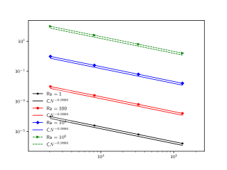
(a) VEM (4.4)-(4.5).

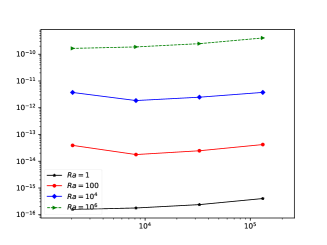
(b) Pressure-robust VEM (4.17)-(4.18).

Figure 1: Error $\|\boldsymbol{\varepsilon}(\boldsymbol{u})-\boldsymbol{\varepsilon}_{h}(\boldsymbol{\Pi}_{h}\boldsymbol{u}_{h})\|_{0}$ of Example 6.1 with $k=2$.

Example 6.2.

Consider the Stokes problem (1.1) on the L-shaped domain $\Omega=(-1,1)\times(-1,1)\setminus[0,1)\times(-1,0]$. The exact solution is taken as

$$\boldsymbol{u} =(2(x^{3}-x)^{2}(3y^{2}-1)(y^{3}-y),(3x^{2}-1)(-2x^{3}+2x)(y^{3}-y)^{2})^{\intercal},$$

$$p =\frac{1}{x^{2}+1}-\frac{\pi}{4}.$$

The exact solution $(\boldsymbol{u},p)$ is smooth although the L-shaped domain $\Omega$ is nonconvex. We present the polygonal mesh and the corresponding numerical velocity flow with $k=2$ in Figure 2. By the numerical results in Table 1, we can see that $\|p-\tilde{p}_{h}\|_{0}=O(h)$, $\|\boldsymbol{\varepsilon}(\boldsymbol{u})-\boldsymbol{\varepsilon}_{h}(\boldsymbol{\Pi}_{h}\tilde{\boldsymbol{u}}_{h})\|_{0}=O(h^{2})$ and $\|p-p_{h}\|_{0}=O(h^{2})$, which coincide with the theoretical error estimates in Theorem 4.3 and Theorem 5.1. The convergence rates of $\|\boldsymbol{u}-\boldsymbol{\Pi}_{h}\boldsymbol{u}_{h}\|_{0}=\|\boldsymbol{u}-\boldsymbol{\Pi}_{h}\tilde{\boldsymbol{u}}_{h}\|_{0}=O(h^{3})$ are higher than the optimal ones on the L-shaped domain, which is probably caused by the uniform meshes. To make the article more concise, here we only show the numerical results of $k=2$. For $k>2$, one can run the test script, named StokesRDFNCVEM2d_example.py, in directory of FEALPy/example [30].

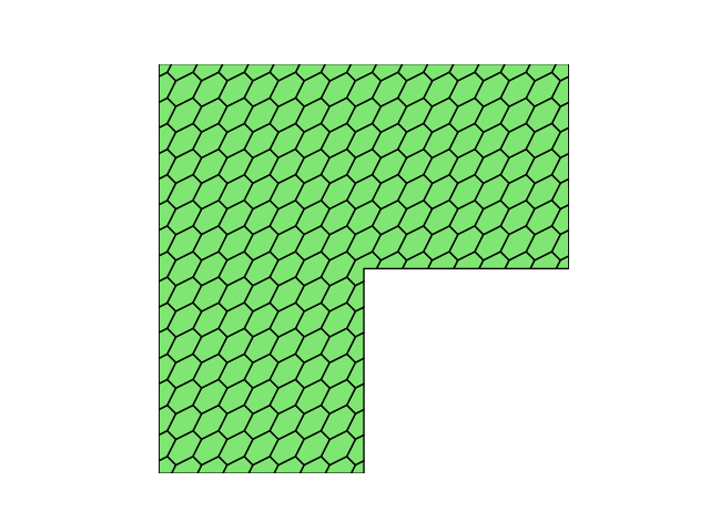
(a) Polygonal mesh.

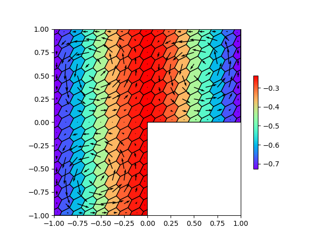
(b) Numerical velocity.

Figure 2: Mesh for L-shaped domain and numerical velocity of Example 6.2 with $k=2$.

Table 1: Numerical results for Example 6.2 with $k=2$.

$\#\mathcal{T}_{h}$	65	225	833	3201
$\|\boldsymbol{u}-\boldsymbol{\Pi}_{h}\tilde{\boldsymbol{u}}_{h}\|_{0}$	3.5827e-03	6.6167e-04	9.2871e-05	1.2026e-05
Order	–	2.44	2.83	2.95
$\|p-\tilde{p}_{h}\|_{0}$	6.5700e-02	3.3869e-02	1.7176e-02	8.6490e-03
Order	–	0.96	0.98	0.99
$\|\boldsymbol{\varepsilon}(\boldsymbol{u})-\boldsymbol{\varepsilon}_{h}(\boldsymbol{\Pi}_{h}\tilde{\boldsymbol{u}}_{h})\|_{0}$	6.7184e-02	2.3092e-02	6.8821e-03	1.8805e-03
Order	–	1.54	1.75	1.87
$\|\boldsymbol{u}-\boldsymbol{\Pi}_{h}\boldsymbol{u}_{h}\|_{0}$	3.5827e-03	6.6167e-04	9.2871e-05	1.2026e-05
Order	–	2.44	2.83	2.95
$\|p-p_{h}\|_{0}$	1.4686e-02	4.2207e-03	1.0318e-03	2.2019e-04
Order	–	1.8	2.03	2.23

References

- [1] P. F. Antonietti, L. Beirão da Veiga, D. Mora, and M. Verani, A stream virtual element formulation of the Stokes problem on polygonal meshes, SIAM J. Numer. Anal., 52 (2014), pp. 386–404.
- [2] T. Apel, V. Kempf, A. Linke, and C. Merdon, A nonconforming pressure-robust finite element method for the Stokes equations on anisotropic meshes, arXiv preprint arXiv:2002.12127, (2020).
- [3] D. N. Arnold, Finite element exterior calculus, Society for Industrial and Applied Mathematics (SIAM), Philadelphia, PA, 2018.
- [4] D. N. Arnold, R. S. Falk, and R. Winther, Finite element exterior calculus, homological techniques, and applications, Acta Numer., 15 (2006), pp. 1–155.
- [5] B. Ayuso de Dios, K. Lipnikov, and G. Manzini, The nonconforming virtual element method, ESAIM Math. Model. Numer. Anal., 50 (2016), pp. 879–904.
- [6] L. Beirão da Veiga, F. Dassi, and G. Vacca, The Stokes complex for virtual elements in three dimensions, Math. Models Methods Appl. Sci., 30 (2020), pp. 477–512.
- [7] L. Beirão da Veiga, C. Lovadina, and G. Vacca, Divergence free virtual elements for the Stokes problem on polygonal meshes, ESAIM Math. Model. Numer. Anal., 51 (2017), pp. 509–535.
- [8] L. Beirão da Veiga, C. Lovadina, and G. Vacca, Virtual elements for the Navier-Stokes problem on polygonal meshes, SIAM J. Numer. Anal., 56 (2018), pp. 1210–1242.
- [9] C. Bernardi, M. Costabel, M. Dauge, and V. Girault, Continuity properties of the inf-sup constant for the divergence, SIAM J. Math. Anal., 48 (2016), pp. 1250–1271.
- [10] D. Boffi, F. Brezzi, and M. Fortin, Mixed finite element methods and applications, Springer, Heidelberg, 2013.
- [11] S. C. Brenner, Korn’s inequalities for piecewise vector fields, Math. Comp., 73 (2004), pp. 1067–1087.
- [12] S. C. Brenner and L. R. Scott, The mathematical theory of finite element methods, Springer, New York, third ed., 2008.
- [13] S. C. Brenner and L.-Y. Sung, Virtual element methods on meshes with small edges or faces, Math. Models Methods Appl. Sci., 28 (2018), pp. 1291–1336.
- [14] A. Cangiani, V. Gyrya, and G. Manzini, The nonconforming virtual element method for the Stokes equations, SIAM J. Numer. Anal., 54 (2016), pp. 3411–3435.
- [15] S. Charnyi, T. Heister, M. A. Olshanskii, and L. G. Rebholz, On conservation laws of Navier-Stokes Galerkin discretizations, J. Comput. Phys., 337 (2017), pp. 289–308.
- [16] L. Chen, J. Hu, and X. Huang, Fast auxiliary space preconditioners for linear elasticity in mixed form, Math. Comp., 87 (2018), pp. 1601–1633.
- [17] L. Chen and X. Huang, Nonconforming virtual element method for th order partial differential equations in , Math. Comp., 89 (2020), pp. 1711–1744.
- [18] L. Chen and F. Wang, A divergence free weak virtual element method for the Stokes problem on polytopal meshes, J. Sci. Comput., 78 (2019), pp. 864–886.
- [19] M. Crouzeix and P.-A. Raviart, Conforming and nonconforming finite element methods for solving the stationary Stokes equations. I, Rev. Française Automat. Informat. Recherche Opérationnelle Sér. Rouge, 7 (1973), pp. 33–75.
- [20] R. G. Durán, An elementary proof of the continuity from to of Bogovskii’s right inverse of the divergence, Rev. Un. Mat. Argentina, 53 (2012), pp. 59–78.
- [21] D. Frerichs and C. Merdon, Divergence-preserving reconstructions on polygons and a really pressure-robust virtual element method for the Stokes problem, arXiv preprint arXiv:2002.01830, (2020).
- [22] P. Hansbo and M. G. Larson, Discontinuous Galerkin and the Crouzeix-Raviart element: application to elasticity, M2AN Math. Model. Numer. Anal., 37 (2003), pp. 63–72.
- [23] X. Huang, Nonconforming virtual element method for -th order partial differential equations in with , Calcolo, 57 (2020), pp. Paper No. 42, 38.
- [24] V. John, A. Linke, C. Merdon, M. Neilan, and L. G. Rebholz, On the divergence constraint in mixed finite element methods for incompressible flows, SIAM Rev., 59 (2017), pp. 492–544.
- [25] A. Linke, On the role of the Helmholtz decomposition in mixed methods for incompressible flows and a new variational crime, Comput. Methods Appl. Mech. Engrg., 268 (2014), pp. 782–800.
- [26] X. Liu, J. Li, and Z. Chen, A nonconforming virtual element method for the Stokes problem on general meshes, Comput. Methods Appl. Mech. Engrg., 320 (2017), pp. 694–711.
- [27] X. Liu, R. Li, and Y. Nie, A divergence-free reconstruction of the nonconforming virtual element method for the Stokes problem, Comput. Methods Appl. Mech. Engrg., 372 (2020), pp. 113351, 21.
- [28] J.-C. Nédélec, Mixed finite elements in , Numer. Math., 35 (1980), pp. 315–341.
- [29] P.-A. Raviart and J. M. Thomas, A mixed finite element method for 2nd order elliptic problems, in Mathematical aspects of finite element methods (Proc. Conf., Consiglio Naz. delle Ricerche (C.N.R.), Rome, 1975), Springer, Berlin, 1977, pp. 292–315. Lecture Notes in Math., Vol. 606.
- [30] H. Wei and Y. Huang, Fealpy: Finite element analysis library in python. https://github.com/weihuayi/fealpy, Xiangtan University, 2017-2021.
- [31] J. Zhao, B. Zhang, S. Mao, and S. Chen, The divergence-free nonconforming virtual element for the Stokes problem, SIAM J. Numer. Anal., 57 (2019), pp. 2730–2759.