Immersed boundary finite element method for blood flow simulation

Abstract

We present an efficient and accurate immersed boundary (IB) finite element (FE) solver for numerically solving incompressible Navier–Stokes equations. Particular emphasis is given to internal flows with complex geometries (blood flow in the vasculature system). IB methods are computationally costly for internal flows, mainly due to the large percentage of grid points that lie outside the flow domain. In this study, we apply a local refinement strategy, along with a domain reduction approach in order to reduce the grid that covers the flow domain and increase the percentage of the grid nodes that fall inside the flow domain. The proposed method utilizes an efficient and accurate FE solver with the incremental pressure correction scheme (IPCS), along with the boundary condition enforced IB method to numerically solve the transient, incompressible Navier–Stokes flow equations. We verify the accuracy of the numerical method using the analytical solution for Poiseuille flow in a cylinder. We further examine the accuracy and applicability of the proposed method by considering flow within complex geometries, such as blood flow in aneurysmal vessels and the aorta, flow configurations which would otherwise be extremely difficult to solve by most IB methods. Our method offers high accuracy, as demonstrated by the verification examples, and high efficiency, as demonstrated through the solution of blood flow within complex geometry on an off-the-shelf laptop computer.

1 Introduction

Immersed boundary methods have been used to simulate flow past rigid and moving/deforming bodies with irregular/complex shapes using Cartesian grids. IB methods, in contrast to mesh-based methods, avoid tedious mesh generation, since they rely on Cartesian grids to solve the governing flow equations, and on discrete set of points (following the literature [1], referred to them as Lagrangian points) for the imposition of prescribed velocity boundary condition. The IB methods are particularly efficient for moving objects and deforming geometries — they are attractive with moving boundaries as they avoid re-meshing — where it does not require the generation a new mesh at each time step, but only the updated position of the points describing the immersed boundary. However, high computational cost of most currently used IB methods in application to internal flows remains a challenge. [2, 3, 4].

1.1 State-of-the art of the existing IB methods

In IB methods, flow equations are discretized on a Cartesian grid that does not conform with the boundaries of the immersed object, and the boundary conditions are imposed indirectly through modifications of the governing Navier–Stokes (N-S) equations. The modification applies as a forcing function in the governing equations that incorporates the presence of the immersed boundary. According to a forcing function $\bm{f}\left(\bm{x,}t\right)$ formulation, the existing IB methods [5] are divided in two groups: continuous (or feedback) forcing and discrete (or direct) forcing methods. These two approaches are often called diffuse and sharp interface methods, respectively.

1.1.1 Continuous forcing approach

In the continuous forcing approach, the forcing function $\bm{f}\left(\bm{x,}t\right)$ is included into the momentum equation (N-S equations). This approach was introduced by Peskin [1, 6] to model blood flow through a beating heart. Peskin’s method is a mixed Eulerian–Lagrangian finite difference method for computing the flow interaction with a flexible immersed boundary. The fluid flow is governed by the incompressible N-S equations, numerically solved on a stationary Cartesian grid, while the immersed boundary is represented by a set of massless elastic fibres. The locations of the fibres is tracked in a Lagrangian fashion by a collection of massless points that move with the local fluid velocity.

Peskin’s method was later applied to rigid bodies by Goldstein et al. [7]. In this method, often called virtual boundary method, the immersed boundary is treated as a fictitious boundary embedded into the fluid. The embedded boundary applies force to the fluid, such that the fluid will be at rest on the surface (no-slip condition). The force $\bm{F}\left(s,t\right)$ on the boundary is computed such that the fluid velocity $\bm{u}\left(\bm{x},t\right)$ satisfies the no-slip condition on the boundary. The body force, is not known a priori and is computed through the velocity on the immersed boundary in a feedback forcing manner.

Saiki and Biringen [8] extended the feedback forcing approach, and eliminated the spurious oscillations caused by the applied feedback forcing term at the boundary. The force $\bm{F}\left(s,t\right)$ on the boundary has been modified, and a more accurate interpolation of the fluid velocity at the boundary points has been developed. A similar approach to the virtual boundary method has been introduced by Lai and Peskin [9]. In this approach, to simulate the flow around a rigid boundary, the boundary is not fixed and undergoes small movement. The immersed boundary points $\bm{X}$ are connected to fixed equilibrium points $\bm{X}^{\text{eq}}$ using a very stiff spring with large stiffness constant. In case the boundary points move away from the desired location, the spring force will pull these boundary points back.

Khadra et al. [10] developed the penalty continuous forcing approach. The main idea, is that the entire flow occurs in a porous medium, governed by the Navier–Stokes–Brinkman equations. The equations contain an additional term of volume drag, called Darcy drag, which accounts for the action of the porous medium on the flow. Su et al. [11] proposed a new implicit force formulation on the Lagrangian marker to ensure exact imposition of no-slip boundary condition at the immersed boundary. The immersed solid boundary is represented by discrete Lagrangian markers, which apply forces to the Eulerian fluid domain. The Lagrangian markers and the fluid variables on the fixed Eulerian grid exchange information through a simple discrete delta function.

Glowinski et al. [12] proposed the distributed Lagrange multiplier method (DLM). The method uses a finite element (FE) method (projection or predictor-corrector method) and introduces Lagrange multipliers (i.e. body force) on the immersed boundary to satisfy the no-slip condition. Lee and LeVeque [13] developed the immersed interface method (IIM), a method that was initially developed for elastic membranes. In the IIM, the boundary force/force strength $\bm{F}\left(\bm{s},t\right)$ is decomposed into tangential and normal components. The interface is explicitly tracked in a Lagrangian manner. The tangential component of the force is included in the momentum equation as an explicit term and the explicit normal boundary force is implemented into the governing equations in terms of a pressure jump condition across the interface [14].

1.1.2 Discrete forcing approach

In the discrete forcing approach, the flow equations are discretized on a Cartesian grid neglecting the immersed boundary. Instead, the discretization at the Cartesian grid points near the immersed boundary is adjusted to account for the presence of the immersed boundary. This discrete approach is is better suited for higher Reynolds numbers, since the velocity boundary conditions at the immersed boundary are imposed without introducing any forcing term.

Mohd-Yusof [15] developed a spectral method, which uses a forcing term that is numerically computed using the difference between the interpolated and the prescribed velocity on the immersed boundary points. This way, the errors between the calculated and the prescribed velocity on the immersed boundary are compensated by the forcing term. Fadlun et al. [16] extended the discrete-time forcing approach introduced by Mohd-Yusof [15] to a three-dimensional finite difference method on a standard marker-and-cell (MAC) staggered grid and showed that the approach was more efficient than feedback-forcing. Balaras [17] proposed a better reconstruction scheme, based on the method of Mohd-Yusof [15] and Fadlun et al. [16], which applies spreading/interpolation along the line normal to the immersed boundary. The algorithm eliminates the ambiguities associated with interpolation along the Cartesian grid lines, but it is limited only to flows with immersed boundaries aligned with one coordinate direction. Gilmanov et al. [18] developed a new reconstruction scheme, which applies to complex, three-dimensional immersed boundaries. The proposed scheme maintains a sharp fluid/immersed boundary interface by discretizing the immersed boundary using an triangular mesh. The numerical solution on the Cartesian grid points close to the immersed boundary points (Lagrangian points) is reconstructed via linear interpolation along the boundary surface normal vector.

Zhang and Zheng [19] developed an improved version of Mohd-Yusof’s method by developing a bilinear interpolation/extrapolation function to interpolate force. Herein, both tangential and the normal velocity components (as opposed to Mohd-Yusof’s method) are used to interpolate force. Therefore, the accuracy in the vicinity of the immersed boundary is enhanced without using higher-order schemes or using body-fitted grids near the immersed boundary. Choi et al. [20] developed a finite-volume immersed boundary method valid to all Reynolds numbers and is suitable for implementation on arbitrary grid topologies. They introduced the concept of tangency correction by decomposing the velocity into tangential and normal components along the outward normal direction to the immersed surface. The tangential velocity component is expressed as a power-law function (which is rather arbitrary) of the wall normal distance.

1.2 Contributions of this study

In the present study we combine the boundary condition-enforced immersed boundary (BCE-IB) method [21, 22] with the incremental pressure correction scheme (IPCS) [23] using the finite element (FE) method. The main advantage of the BCE-IB method is that it satisfies accurately both the the governing equations and boundary conditions using velocity and pressure correction procedures. The velocity correction applies implicitly such that the velocity on the immersed boundary (Lagrangian points) interpolated from the corrected velocity values computed on the mesh nodes (Eulerian nodes) accurately satisfies the prescribed velocity boundary conditions. The incremental pressure correction scheme (IPCS) is a modified version of projection method, which provides improved accuracy at little extra computational cost. We implement the method using FEniCS [24] (an open-source software package that solves partial differential equations) to numerically solve the incompressible Navier-Stokes equations. The proposed IB scheme applies to both external and internal flows, but in the present study we are particularly interested in internal flow problems.

Our numerical scheme, increases the computational efficiency of the IB method for internal flow cases, by reducing the number of unused elements through a sophisticated and efficient mesh refinement inside the immersed boundary. Reducing the computational cost is of paramount importance for IB methods applied to internal flows, since the advantageous features of IB methods, that have made them popular for external flow simulations, do not entirely apply for internal flows. Users of IB methods are aware of this problem and have come up with various strategies to circumvent this liability [2, 3, 4].

The remainder of the paper is organized as follows. In Section 2, we present the numerical formulation for the proposed immersed boundary (IB) method. In Section 3, we solve benchmark problems to verify the accuracy of the proposed IB method. Section 4 is concerned with the numerical examples that demonstrate the accuracy and applicability of the proposed IB method. Section 5 contains conclusions.

2 Numerical formulation of the proposed immersed boundary method

2.1 Governing equations

We consider the incompressible viscous flow in a spatial domain $\Omega$, which contains an immersed boundary in the form of a closed surface $\partial S$. The immersed boundary is modeled as localized body forces acting on the surrounding fluid. The incompressible N-S equations — in their primitive variables (velocity $\bm{u}$ and pressure $p$) formulation — accounting for the immersed boundary are written as:

$$\rho\left(\frac{\partial\bm{u}}{\partial t}+\bm{u}\cdot\bm{\nabla}\bm{u}\right)=-\nabla p+\nabla\cdot 2v\bm{\varepsilon}(\bm{u})+\bm{f},$$ (1)

$$\nabla\cdot\bm{u}=0,$$ (2)

subject to the no-slip boundary condition on $\partial S$

$$\bm{u}(\bm{X}(s),t)=\bm{U}_{B},$$ (3)

with $\bm{U}_{B}$ being the prescribed velocity of the immersed boundary, and $v$ the kinematic viscosity of the fluid. The term $\bm{\varepsilon}(\bm{u})$ is the strain-rate tensor defined as:

$$\bm{\varepsilon}(\bm{u})=\frac{1}{2}\left(\nabla\bm{u}+\left(\nabla\bm{u}\right)^{\mathrm{T}}\right).$$ (4)

The forcing term $\bm{f}$ is added to the right hand side (RHS) of the momentum Eq.(1) to account for the presence of the immersed boundary. The forcing term $\bm{f}\left(\bm{x},t\right)$ is the local body force density at the fluid nodes (Eulerian nodes), it is distributed from the surface force density $\bm{F}\left(s,t\right)$ ($s$ is a parametrization of the immersed boundary surface) at the immersed boundary points (Lagrangian points – we use traditional terminology used in [22]). The forcing term is expressed as:

$$\bm{f}(\bm{x},t)=\int_{\partial S}\bm{F}(\bm{s},t)\,\delta\left(\bm{x}-\bm{X}(s,t)\right)\mathrm{d}s,$$ (5)

where $\bm{x}$ and $\bm{X}\left(s\bm{,}t\right)$ denote the Eulerian nodes and Lagrangian point coordinates that discretize the fluid domain and the immersed boundary, respectively. Eulerian nodes and Lagrangian points interact through Dirac delta function $\delta\left(\bm{x}-\bm{X}\left(s,t\right)\right)$. Therefore, the velocity at the immersed boundary points is calculated from the velocity at the Eulerian nodes using the Dirac delta function

$$\bm{U}(\bm{X}(s,t))=\int_{\Omega}\bm{u}(\bm{x})\,\delta\left(\bm{x}-\bm{X}(s,t)\right)\mathrm{d}V.$$ (6)

2.2 Incremental Pressure Correction Scheme (IPCS)

The Incremental Pressure Correction Scheme (IPCS) [23] is an operator splitting method, which transforms the nonlinear Navier–Stokes (N-S) equations into algebraic equations by coupling the pressure and velocity field values (N-S equations are difficult to solve due to their inherent non-linearity). IPCS is a modified version of the fractional step method proposed by Chorin [25] and Témam [26]. It improves the accuracy of the original scheme with little extra cost. In our description we consider no external forces for the N-S equations, and in Section 2.3 we explain in detail how IB forces were incorporated.

The IPCS scheme involves three steps. In the first step, we compute a tentative velocity $\bm{u}^{*}$ by advancing the linear momentum Eq.(1) in time using the backward Euler difference scheme, $\dot{\bm{u}}=\frac{\bm{u}^{n+1}-\bm{u}^{n}}{\Delta t}$. We linearize the nonlinear terms using a semi-implicit method, such that the advection term $\bm{u}\cdot\bm{\nabla}\bm{u}$ becomes $\bm{u}^{n}\cdot\bm{\nabla}\bm{u}^{n+1}$. Using this semi-implicit approach for linearization the Courant-Friedrichs-Lewy (CFL) condition, which limits the time step according to the velocity and spatial discretization to ensure stability of the solution, becomes less restrictive. Additionally, the kinematic viscosity is written as $v=v\left(\bm{u}^{n}\right)$, which simplifies the N-S equations that are now written as a linearized set of equations, known as the Oseen equations:

$$\bm{u}^{n+1}+\Delta t\bm{u}^{n}\cdot\nabla\bm{u}^{n+1}-\Delta t\nabla\cdot 2v\bm{\varepsilon}(\bm{u}^{n+1})+\Delta t\nabla p^{n+1}=\bm{u}^{n},$$ (7)

$$\nabla\cdot\bm{u}^{n+1}=0.$$ (8)

In Eq.(7), $p^{n+1}$ is still unknown. Therefore, we will compute the tentative velocity $\bm{u}^{*}$ ($\bm{u}^{*}\approx\bm{u}^{n+1}$), by replacing in Eq.(7) $p^{n+1}$ with the known value $p^{n}$. This makes Eq.(7) easier to solve for the tentative velocity $\bm{u}^{*}$:

$$\bm{u}^{*}+\Delta t\,\bm{u}^{n}\cdot\nabla\bm{u}^{n+1}-\Delta t\,\nabla\cdot 2v\bm{\varepsilon}\left(\bm{u}^{*}\right)+\Delta t\,\nabla p^{n}=\bm{u}^{n}.$$ (9)

Equation (9) is numerically solved to compute the tentative velocity $\bm{u}^{*}$ without using the incompressibility constraint Eq.(2).

In the second step, we use the tentative velocity $\bm{u}^{*}$ to compute the updated velocity $\bm{u}^{n+1}$, which is divergence-free (and should fulfill the incompressibility constraint). We define a function for the velocity correction as $\bm{u}^{c}=\bm{u}^{n+1}-\bm{u}^{*}$, and after some algebra (subtracting Eq.(9) from Eq.(7)) and using that $\bm{\nabla}\cdot\bm{u}^{n+1}=0\Rightarrow\ \bm{\nabla}\cdot\bm{u}^{c}=-\bm{\nabla}\cdot\bm{u}^{*}$ (incompressibility constraint) we obtain a new set of flow equations for $\bm{u}^{c}$:

$$\bm{u}^{c}+\Delta t\,\bm{u}^{n}\cdot\nabla\bm{u}^{c}-\Delta t\,\nabla\cdot 2v\bm{\varepsilon}\left(\bm{u}^{c}\right)+\Delta t\,\nabla\Phi^{n+1}=0,$$ (10)

$$\nabla\cdot\bm{u}^{c}=-\nabla\cdot\bm{u}^{*},$$ (11)

where $\Phi^{n+1}=p^{n+1}-p^{n}$. Equation (10) can be further simplified to $\bm{u}^{c}\bm{+}\Delta\text{t\ }\bm{\nabla}\Phi^{n+1}\bm{=0}$ and the system of Eqs.(10)-(11) is reduced to an elliptic type (Poisson) partial differential equation for the pressure difference $\Phi^{n}$

$$\nabla^{2}\Phi^{n+1}=\frac{\nabla\cdot\bm{u}^{*}}{\Delta t},$$ (12)

with boundary conditions being those applied to the original flow problem.

In the third and final step, we compute the updated velocity $\bm{u}^{n+1}$ and pressure $p^{n+1}$ through $p^{n+1}=\Phi^{n+1}+p^{n}$ and $\bm{u}^{n+1}=\bm{u}^{*}+\Delta t\bm{\nabla}\Phi^{n+1}$, respectively.

The algorithmic procedure for our implementation of the IPCS for solving N-S equations is summarized below:

1. Calculate the tentative velocity $\bm{u}^{*}$ by solving Eq.(9)

2. Solve the Poisson equation $\bm{}\nabla^{2}\Phi^{n+1}\bm{=}\frac{\nabla\cdot\bm{u}^{*}}{\Delta t}$ (Eq.(12))

3. Calculate the corrected velocity $\bm{u}^{n+1}=\bm{u}^{*}+\Delta t\bm{\nabla}\Phi^{n+1}$ and pressure $p^{n+1}=\Phi^{n+1}+p^{n}.$

2.3 Boundary Condition Enforced Immersed Boundary (BCE-IB) method

In this section, we describe the boundary condition enforced immersed boundary (BCE-IB) method for the numerical solution of the incompressible 3D Navier–Stokes equations.

The immersed boundary method has two steps:

• Predictor step: where we numerically solve the N-S equations to compute the predicted velocity field $\tilde{\bm{u}}\left(\bm{x}\right)$ by disregarding the body force terms in Eq.(1) ($\bm{f}=\bm{0}$)

$$\rho\frac{\tilde{\bm{u}}-\bm{u}^{n}}{\Delta t}+\rho\left(\bm{u}^{n}\cdot\nabla\bm{u}^{n}\right)=+\Delta t\nabla p^{n}-\Delta t\nabla\cdot 2v\bm{\varepsilon}(\bm{u}^{n})$$ (13)

• Corrector step: where we account for the effect of body forces and update the predicted velocity field $\tilde{\bm{u}}$ to the updated one $\bm{u}^{n+1}$, which satisfies the boundary condition $\bm{u}\left(\bm{X}\left(s\right),t\right)=\bm{U}_{B}$

$$\rho\frac{\bm{u}^{n+1}-\tilde{\bm{u}}}{\Delta t}=\bm{f}^{n+1}.$$ (14)

In the predictor step, Eq.(13) is used to compute the predicted velocity field $\tilde{\bm{u}}$ under the incompressibility constraint (mass conservation), which couples the velocity and pressure. The predictor step accounts for the first of the three steps in the IPCS method. In this step, we compute the predicted velocity $\tilde{\bm{u}}$, which in this case is the tentative velocity $\bm{u}^{*}$ (Step 1 in the IPCS algorithmic procedure). The corrector step, involves the evaluation of the unknown body force $\bm{f}^{n+1}$ and the update of the predicted velocity $\tilde{\bm{u}}$ to the physical one $\bm{u}^{n+1}$ (Steps 2 and 3 in the IPCS algorithmic procedure).

Accurate and efficient computation of the unknown body force $\bm{f}^{n+1}$ is an important advantage of the Boundary Condition Enforced Immersed Boundary (BCE-IB) method. In this method, the body force $\bm{f}^{n+1}$ is equivalent to a velocity correction, which applies implicitly such that the velocity $\bm{U}\left(\bm{X}\left(s\right),t\right)$ on the Lagrangian points, interpolated from the physical velocity $\bm{u}\left(\bm{x},t\right)$ computed on the Eulerian nodes, equals to the prescribed boundary velocity $\bm{U}_{B}$ (Eq. (3)). The body force term $\bm{f}^{n+1}$ is computed using the equation

$$\bm{U}_{B}^{n+1}\left(\bm{X}^{n+1}\right)=\int_{\Omega}\left(\tilde{\bm{u}}+\Delta t\frac{\bm{f}^{n+1}}{\rho}\right)\delta\left(\bm{x}-\bm{X}^{n+1}\right)\mathrm{d}V,$$ (15)

derived by substituting Eq.(14) to Eq.(6). The force density $\bm{f}^{n+1}\left(\bm{x},t\right)$, is evaluated on the Eulerian nodes, and it is computed by distributing (‘spreading’) the boundary force $\bm{F}\left(\bm{X}\left(s\right),t\right)$ on the Lagrangian points through the Dirac delta function $\delta\left(\bm{x-X}\left(s,t\right)\right)$ (see Eq.(5)). Eq.(15) is written as

$$\bm{U}_{B}^{n+1}\left(\bm{X}^{n+1}\right)=\int\left(\tilde{\bm{u}}+\Delta t\frac{\int{\bm{F}^{n+1}\left(\bm{X}^{n+1}\right)\delta\left(\bm{x}-\bm{X}^{n+1}\right)\mathrm{d}s}}{\rho}\right)\delta\left(\bm{x}-\bm{X}^{n+1}\right)\mathrm{d}V,$$ (16)

and $\bm{U}_{B}^{n+1}$ is no longer correlated with $\bm{f}^{n+1}$ but instead with $\bm{F}^{n+1}$.

To compute the boundary force $\bm{F}^{n+1}$, we rewrite Eq.(16) in a discrete form that results in an algebraic system of equations. We represent the immersed boundary by a set of Lagrangian points $\bm{X}_{i}=\left(X_{i},Y_{i},Z_{i}\right),\ i=1,2,\ldots,M$ and the flow domain by the Eulerian nodes $\bm{x}_{j}=\left(x_{j},y_{j},z_{j}\right),\ j=1,2,\ldots,N$. In our analysis, the Eulerian mesh in the vicinity of the immersed object has a uniform Cartesian grid structure with grid spacing $h$. Furthermore, the Dirac function $\delta\left(\bm{x}-\bm{X}\left(s,t\right)\right)$ is approximated by a continuous kernel distribution $D\left(\bm{x}_{i}-\bm{X}^{j}\right)$ given as

$$D_{ij}=D\left(\bm{x}_{i}-\bm{X}^{j}\right)=\left(\frac{1}{h}\delta\left(\frac{x_{i}-X^{j}}{h}\right)\right)\left(\frac{1}{h}\delta\left(\frac{y_{i}-Y^{j}}{h}\right)\right)\left(\frac{1}{h}\delta\left(\frac{z_{i}-Z^{j}}{h}\right)\right),$$ (17)

with the kernel $\delta\left(r\right)$ proposed by Lai and Peskin [9]

$$\delta(r)=\begin{cases}\begin{aligned} \frac{1}{8}\left(3-2|r|+\sqrt{1+4|r|-4r^{2}}\right),&\quad&|r|&\leq 1\\ \frac{1}{8}\left(5-2|r|-\sqrt{-7+12|r|-4r^{2}}\right),&\quad&1<|r|&\leq 2\\ 0,&\quad&|r|&>2\end{aligned}\end{cases}$$ (18)

Using Eq.(6) for the force term

$$\bm{f}^{n+1}(\bm{x}_{j})=\sum_{i=1}^{M}{\bm{F}^{n+1}\left(\bm{X}_{i}^{n+1}\right)D_{h}^{ij}\Delta S_{i}},$$ (19)

Eq.(16) is written as

$$\bm{U}_{B}^{n+1}(\bm{X}_{i}^{n+1})=\sum_{j=1}^{N}\tilde{\bm{u}}(\bm{x}_{j})D_{h}^{ij}h^{3}+\sum_{j=1}^{N}\sum_{k=1}^{M}\frac{\bm{F}^{n+1}(\bm{X}_{i}^{n+1})\Delta t}{\rho}D_{h}^{kj}D_{h}^{ij}h^{3},$$ (20)

where $\Delta S_{i}$ is the area of the i^th surface element (segment). Eq.(20) forms a well-defined system of equations for the variables $\bm{F}_{i}^{n+1}\bm{\ }\left(i=1,2,\ldots,M\right)$. Eq.(20) can be written in matrix notation as

$$\bm{A}_{\bm{F}}\bm{F}=\bm{B}_{\bm{F}},$$ (21)

with $\bm{A}_{\bm{F}},\bm{F}$ and $\bm{B}_{\bm{F}}$ defined as

$$\bm{A}_{\bm{F}}=\frac{\Delta t}{\rho}h^{3}\begin{bmatrix}D_{11}\Delta S_{1}&D_{12}\Delta S_{1}&\dots&D_{1N}\Delta S_{1}\\ D_{21}\Delta S_{2}&D_{22}\Delta S_{2}&\dots&D_{2N}\Delta S_{2}\\ \vdots&\vdots&\ddots&\vdots\\ D_{M1}\Delta S_{M}&D_{M2}\Delta S_{M}&\dots&D_{MN}\Delta S_{M}\end{bmatrix}\begin{bmatrix}D_{11}&D_{12}&\dots&D_{1M}\\ D_{21}&D_{22}&\dots&D_{2M}\\ \vdots&\vdots&\ddots&\vdots\\ D_{N1}&D_{N2}&\dots&D_{NM}\end{bmatrix},$$ (22)

$$\bm{B}_{\bm{F}}=\bm{U}-h^{3}\bm{D}^{\mathrm{T}}\tilde{\bm{u}}=\begin{bmatrix}\bm{U}_{1}\\ \bm{U}_{2}\\ \vdots\\ \bm{U}_{M}\end{bmatrix}-h^{3}\begin{bmatrix}D_{11}&D_{21}&\dots&D_{N1}\\ D_{12}&D_{22}&\dots&D_{N2}\\ \vdots&\vdots&\ddots&\vdots\\ D_{1M}&D_{2M}&\dots&D_{NM}\end{bmatrix}\begin{bmatrix}\tilde{\bm{u}}_{1}\\ \tilde{\bm{u}}_{2}\\ \vdots\\ \tilde{\bm{u}}_{N}\end{bmatrix},$$ (23)

$$\bm{F}=\begin{bmatrix}\bm{F}_{1}\\ \bm{F}_{2}\\ \vdots\\ \bm{F}_{M}\end{bmatrix},$$ (24)

where $\bm{U}_{i}\ (i\bm{=}1,2,\ldots,M\bm{)}$, $\bm{F}_{i}\bm{\ (}i\bm{=}1,2,\ldots,M\bm{)}$ and ${\tilde{\bm{u}}}_{j}\bm{\ }\left(j=1,2,\ldots,M\right)$ are the abbreviations for $\bm{U}_{B}^{n+1}\left(\bm{X}_{\bm{i}}^{n+1}\right)$, $\bm{F}^{n+1}\left(\bm{X}_{\bm{i}}^{n+1}\right)$ and $\tilde{\bm{u}}\left(\bm{x}_{j}\right)$, respectively. By solving he system of equations (Eq.(22)) using a direct solver, we obtain the unknown boundary force $\bm{F}_{\bm{i}}^{n+1}\bm{\ }\left(i=1,2,\ldots,M\right)$ at all Lagrangian points. Boundary forces $\bm{F}_{\bm{i}}^{n+1}$ are then substituted into Eq.(19) and Eq.(16) to calculate the body force $\bm{f}^{n+1}$ on the Eulerian nodes, and the corrected physical velocity $\bm{u}^{n+1}$.

2.4 Algorithmic procedure

Our approach combines the IPCS (section 2.2) with the BCE-IB method (section 2.3). The velocity field predicted by IPCS is corrected to account for the force contribution from the immersed boundary. The proposed solution procedure can be summarized as follows; to update the solution from time instance $n$ to $n+1$:

1. Calculate the tentative velocity $\tilde{\bm{u}}$ using Eq.(13)

2. Compute the matrix $\bm{A}_{\bm{F}}$ using Eq.(22)

3. Solve the system (Eq.(21)) to compute the boundary force $\bm{F}^{n+1}\left(\bm{X}_{i}^{n+1}\right)\bm{,\ (}i\bm{=}1,2,\ldots,M\bm{)}$ on the Lagrangian points. Substitute the computed boundary force $\bm{F}^{n+1}\left(\bm{X}_{i}^{n+1}\right)$ into Eq.(19) to obtain the body force $\bm{f}^{n+1}\left(\bm{x}_{j}^{n+1}\right)\bm{,\ (}j\bm{=}1,2,\ldots,N\bm{)}$ on the Eulerian points.

4. Use $\tilde{\bm{u}}$ to update the corrected velocity $\bm{u}^{(n+1)}=\frac{\Delta t\bm{f}^{n+1}+\tilde{\bm{u}}}{\rho}$ using Eq.(14)

5. Solve the Poisson equation $\bm{}\nabla^{2}\Phi^{n+1}\bm{=}\frac{\nabla\cdot\bm{u}^{n+1}}{\Delta t}$ for $\Phi^{n}$ (Eq.(12))

6. Recompute the updated velocity $\bm{u}^{n+1}=\bm{u}^{n}+\Delta t\bm{\nabla}\Phi^{n+1}$ and pressure $p^{n+1}=\Phi^{n+1}+p^{n}.$

7. Set physical/updated velocity $\bm{u}^{\left(n+1\right)}$ as $\bm{u}^{\left(n\right)}$ and repeat steps (1) to (4) until the desired solution is achieved.

Steps 1, 5, 6 apply to the IPCS method without the presence of the immersed boundary, while Steps 2, 3, 4 calculate the velocity field (on the Eulerian nodes) due to the presence of the immersed boundary.

2.5 Surface area for Lagrangian points

In 3D flow cases, the surface area ${\Delta S}_{i}$ that is assigned to each Lagrangian point is not as straightforward to define as in two dimensions. Immersed boundaries are represented by a set of Lagrangian points. Therefore, the number of these points and the way they are distributed over the immersed boundary directly affect the accuracy of the IB method.

In 2D, the distribution and number of Lagrangian points are always investigated through the ratio of $\frac{\text{ds}}{h}$, with ds being spacing of the Lagrangian points and $h$ the Eulerian nodal spacing. High ratio of $\frac{\text{ds}}{h}$ will cause fluid leakage (spreading from Lagrangian points to Eulerian nodes and vice-versa is not accurate), while low ratio will increase the computational cost (as rows in matrix $\bm{A}_{\bm{F}}$ in Eq.(21) will be linearly dependent and the matrix will become ill-conditioned and therefore difficult to invert). In the literature, there are many studies which report on selection of $\frac{\text{ds}}{h}$; Uhlmann [27] suggests that Lagrangian points spacing should be equal to the Eulerian mesh/grid resolution $\frac{\text{ds}}{h}=1$, Su et al. [11] and Kang and Hassan [28] used $\frac{\text{ds}}{h}=1.5$ (Lagrangian points spacing is larger than the Eulerian mesh/grid resolution), while Lima E Silva et al. [29] reported $\frac{\text{ds}}{h}\leq 0.9$ (Lagrangian points spacing is less than the Eulerian nodal resolution). In 3D, the surface area ${\Delta S}_{i}$ appears as a key feature of the IB method. In this study, we propose and use an easy to apply method to compute ${\Delta S}_{i}$. The area of each surface element ${\Delta s}_{i}$ should be close to $(ah)^{2}$, with $0.1\leq a\leq 2.5$ (just like having in 2D $0.3\leq\frac{ds}{h}\leq 2.5$, with $h$ being the spacing of the Eulerian nodes).

In this study, we uniformly distribute the Lagrangian points to assign the same value $\Delta S$ to all Lagrangian points. To obtain a distribution of Lagrangian points with uniform surface element area, we generate surface mesh (the nodes are the Lagrangian points used in the IB method) with element edges having lengths with small standard deviation. The area element $\Delta S$ for each Lagrangian point is the computed mean value of the facets area.

2.6 Derived quantities—wall shear stress (WSS)

An important aspect of blood flow simulations is the numerical computation of flow parameters that are of clinical importance, such as blood vessel wall shear stress (WSS). While focusing on WSS, we present an accurate meshless point collocation to compute derived quantities from the velocity field obtained from blood flow simulations. Meshless methods (MMs) have been well-established for the efficient and accurate representation of 3D complex geometries as point clouds, and for the accurate computation of spatial derivatives. In our study, we use the Discretization Corrected Particle Strength Exchange (DC PSE) [30] meshless method. The DC PSE method, is one of the most accurate meshless point collocation methods to compute spatial derivatives of field functions defined on point clouds.

WSS is defined as the magnitude of the surface traction vector $\bm{t}_{\bm{s}}=\bm{t}-(\bm{t}\cdot\hat{\bm{n}})\cdot\hat{\bm{n}}$, where $\hat{\bm{n}}$ is the unit normal vector pointing outward, and $\bm{t}=2\mu{\bm{\varepsilon}}$ is the shear stress, defined based on the fluid’s viscosity $\mu$ and the rate of deformation tensor ${\bm{\varepsilon}}$. Let $\bm{u}\left(\bm{x},t\right)$ be continuously differentiable velocity vector field describing the blood flow at a point in the domain of interest. The velocity field values are computed by interpolating the velocity field computed on the Cartesian flow domain using the IB method, on a body-fitted mesh of the immersed object (the mesh is used only for visualization of the flow field and derived quantities such as WSS).We consider a discretization of the domain of interest (immersed object) using a finite-element mesh (tetrahedral linear elements), and denote the corresponding set of nodes by $N$. The nodal subset $N_{S}$ with points on the surface of the tetrahedral mesh will be used for the calculation of WSS. Using indicial notation for the components of $\bm{u}$, the deformation (strain-rate) tensor components are defined by ${{\varepsilon}}_{{ij}}=\frac{1}{2}\left(u_{i,j}+u_{j,i}\right)$ for $i,j=\left\{x,y,z\right\}$, where $u_{i,j}=\frac{\partial u_{i}}{\partial x_{j}}$. The terms $\frac{\partial u_{i}}{\partial x_{j}}$ of the deformation tensor ${\bm{\bm{\varepsilon}}}$ are computed on the surface points $N_{S}$ using the DC PSE method as

$$\frac{\partial u_{i}}{\partial x_{j}}=\Phi_{,j}u_{i},$$ (25)

with $\Phi_{,j}$ being the j^th spatial derivative computed, and $u_{i}$ being a column vector of the i^th velocity vector components.

3 Algorithm verification

We demonstrate the accuracy, efficiency and applicability of our method on internal flow cases. The numerical results obtained were compared against analytical solutions (where available) and experimental data. We consider two 3D benchmark flown problems, the Poiseuille flow in a straight tube and the angle tube bend flow problem, where an analytical solution (Poiseuille flow) and experimental data (tube bend) are available, respectively.

3.1 Poiseuille flow in a cylindrical tube

We demonstrate the accuracy of the proposed IB method considering the Poiseuille flow in a straight cylindrical tube. The tube has length $L=10R$ and radius $R=0.005$ m, and is immersed in a domain (which is the spatial domain where the flow equations are solved) with dimensions $-0.006\ m\leq y,z\leq 0.006\ m$ and $0\ m\leq x\leq 0.05\ m$, as shown in Fig. 1. The immersed cylinder is described by a set of points on its surface (Lagrangian points). The box domain is discretized with a high quality tetrahedral mesh. The vertices of the tetrahedral elements (Eulerian nodes) form a uniform Cartesian grid. To generate the mesh we use the FEniCS build-in function BoxMesh [24].

Figure 1: (a) Flow domain for the Poiseuille flow example with inlet (circle in red color), outlet (circle in green color) and walls (yellow color) boundaries; (b) wireframe of the tetrahedral mesh and the immersed boundary (Lagrangian points); (c) vertical cross-section of the tetrahedral mesh along with the immersed boundary.

The driving force of the flow is the pressure difference applied to the inlet and outlet. In our simulations, the density of the fluid was set to $\rho=1,050~{}\mathrm{kg\,m^{-3}}$, and the dynamic viscosity to $\mu=0.00345~{}\mathrm{N\,s/m^{2}}$. At the inlet (red circle in Fig. 1a) and outlet (green circle in Fig. 1a), we apply pressure boundary conditions, while at the remaining walls (surface yellow Fig. 1a), we apply no-slip velocity boundary conditions ($\bm{u}=0$). The time step was set to $dt=2.5\times 10^{-3}$. The simulation ends when the normalized root mean square difference

$$L_{\text{NRMSE}}=\frac{\sqrt{\frac{\sum_{i=1}^{N}\left(u_{i}^{t+dt}-u_{i}^{t}\right)^{2}}{N^{2}}}}{\left(\max\left(u_{i}^{t}\right)-\min\left(u_{i}^{t}\right)\right)},$$ (26)

between two successive time instances for all three velocity components is less than $10^{-8}$ (practically, the flow reaches a steady state). The exact solution for the velocity field components is $u_{x}=u_{y}=0$ and $u_{z}\left(r\right)=U_{\max}\left(1-\left(\frac{r}{R}\right)^{2}\right)$, with $U_{\max}=-\frac{R^{2}}{4\mu}\frac{\text{dp}}{\text{dz}}$ being the maximum velocity. By setting the pressure difference to $\frac{\text{dp}}{\text{dz}}=\frac{1}{L}$ (applying $p_{\text{inlet}}=1$ and $p_{\text{outlet}}=0$) the Reynolds number becomes $\mathrm{Re}=\frac{U_{\max}L}{\mu}\approx 551$, while for $p_{\text{inlet}}=2$ Reynolds number becomes $\mathrm{Re}=\frac{U_{\max}L}{\mu}\approx 1,102$.

Table 1: Tetrahedral mesh resolution, number of Eulerian nodes, number of tetrahedral elements, and number of Lagrangian points for the successively denser grids considered for the Poiseuille flow problem.

Grid resolution $h$ (m)	Eulerian nodes	Tetrahedral elements	Lagrangian pointss
$1\times 10^{-3}$	8,619	43,200	1,632
$5\times 10^{-4}$	63,125	345,600	6,464
$2.5\times 10^{-4}$	482,601	2,764,800	25,527

We use successively denser tetrahedral meshes to obtain a mesh independent numerical solution. The meshes are described in Table 1. Table 2, reports the maximum absolute error $L_{\infty}=\underset{i}{\max}\left|u_{i}^{\text{numerical}}-u_{i}^{\text{exact}}\right|$ and the root mean square error (RMSE) $L_{2}=\frac{1}{N}\sqrt{\sum_{i=1}^{N}\left(u_{i}^{\text{numerical}}-u_{i}^{\text{exact}}\right)^{2}}$ for different mesh resolution, for $\mathrm{Re}=551$ and $\mathrm{Re}=1,102$. For $\mathrm{Re}=551$ the convergence rates for the $L_{\infty}$ and $L_{2}$ error norms are 1.29 and 2.79, respectively. The convergence rates for $L_{\infty}$ and $L_{2}$ error norms do not change, demonstrating that the relative error does not change.

Table 2: Maximum absolute $L_{\infty}$ and root mean square $L_{2}$ error norms for the numerical solution computed using the proposed IB method and the analytical solution for the Poiseuille flow example using $\mathrm{Re}=551$ and $\mathrm{Re}=1,102$.

$\mathrm{Re}=551$		$\mathrm{Re}=1,102$
$L_{\infty}$	$L_{2}$	$L_{\infty}$	$L_{2}$
$1.47\times 10^{-2}$	$1.99\times 10^{-4}$	$2.95\times 10^{-2}$	$3.99\times 10^{-4}$
$6.62\times 10^{-3}$	$3.07\times 10^{-5}$	$6.62\times 10^{-3}$	$6.18\times 10^{-5}$
$2.44\times 10^{-3}$	$4.15\times 10^{-6}$	$4.89\times 10^{-3}$	$8.42\times 10^{-6}$

Figure 2 shows the $L_{\infty}$ and $L_{2}$ error norms versus the mesh resolution of the Eulerian mesh. For both $\mathrm{Re}=55$1 and $\mathrm{Re}=1,102$, both $L_{\infty}$ and $L_{2}$ error norms, the results suggest that the proposed scheme is accurate.

Figure 2: Maximum absolute $L_{\infty}$ (red line) and root mean square $L_{2}$ (black line) error norms versus Eulerian tetrahedral mesh resolution $h$ for the Poiseuille flow example.

Figure 3 shows the velocity streamlines for $\mathrm{Re}=551$ and $\mathrm{Re}=1,102$. The streamlines were produced on a tetrahedral body-fitted mesh (we refer to as visualization mesh) that consist of 345,600 linear elements. The velocity field computed with the IB method on the Eulerian nodes has been projected on the visualization mesh for visualization purposes (the visualization mesh is not used in the computation of the velocity and pressure field).

Figure 3: Velocity streamlines for (a) $\mathrm{Re}=551$ and (b) $\mathrm{Re}=1,102$ using a visualization mesh of 345,600 linear elements for the Poiseuille flow example. The maximum velocity computed for $\mathrm{Re}=551$ and $\mathrm{Re}=1,102$ was 0.0361 and 0.0723, respectively (the theoretical values are 0.0362 and 0.0724, respectively)

3.2 3D angle tube bend

We further demonstrate the accuracy of the proposed method, considering the flow in a three-dimensional 90° angle tube bend, as shown in Fig. 4. We use this flow example to demonstrate the ability of the proposed method to accurately capture flows in tortuous tubes where secondary flows can occur. For U-bend, flow data are available; Van De Vosse et al. [31] performed laser Doppler velocimetry experiments to obtain the center-plane axial velocities at a set of different angles around the tube bend. To reduce disturbances in the flow field due to inflow boundary conditions, we extended the inlet and outlet by 1 mm. In our numerical simulations, we set the Reynolds number—computed based on the tube inner diameter $D_{i}$ and the mean inlet velocity $\overline{U}$—to $\mathrm{Re}=300$, to match the experimental conditions. The inner diameter $D_{i}$ and the curvature radius $R$ of the tube were set to 4 and 24 mm, respectively.

Figure 4: U-bend geometry (a) top and (b) side view. The points on the surface define the Lagrangian points of the immersed boundary $R_{D}=1\ mm$, $R=24\ mm$, $D_{i}=4\ mm$.

The U-bend geometry is embedded within a box domain with dimensions $-0.0064\ m\leq x\leq 0.032\ m$, $0\ m\leq y\leq 0.0384\ m$ and $-0.0064\ m\leq z\leq 0.0064\ m$, as shown in Fig. 5b. We discretize the flow domain using tetrahedral elements. The box domain is discretized with a high quality tetrahedral mesh (the vertices of the tetrahedral elements are the Eulerian nodes), generated using a uniform Cartesian grid (to generate the mesh we used the FEniCS build-in function BoxMesh).

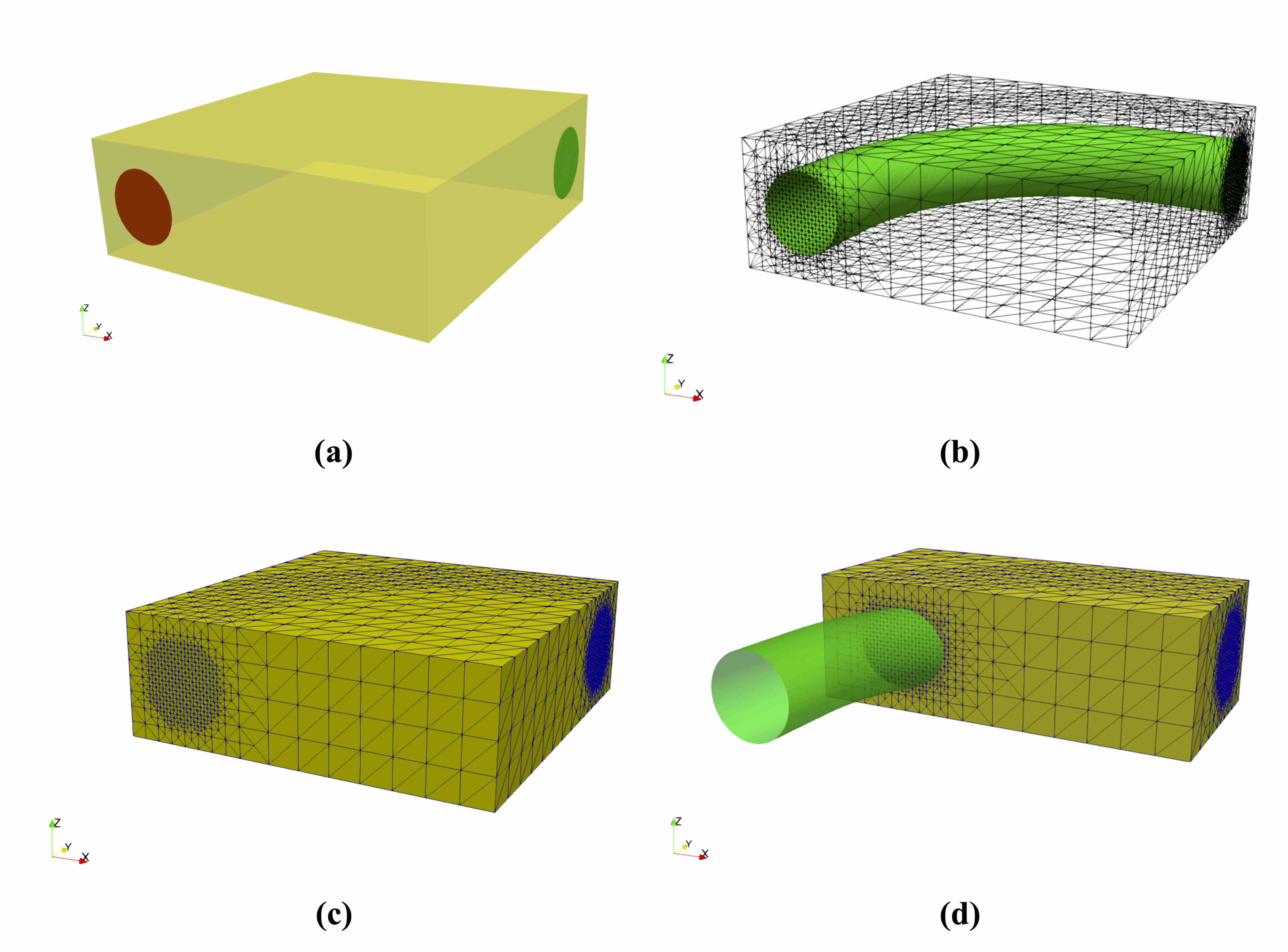
Figure 5: (a) Flow domain for the U-bend flow example, with inlet (circle in red color), outlet (circle in green color) and walls (yellow color) boundaries; (b) wireframe of the tetrahedral mesh and the U-bend immersed boundary (Lagrangian points); (c) tetrahedral mesh refined close and inside the immersed boundary, and (d) vertical cross-section of the tetrahedral mesh.

The tetrahedral mesh is locally refined in the vicinity and within the interior of the immersed boundary, using the FEniCS built-in function $\it{Refine}$ [24] which uses the algorithm by Plaza and Carey [32]. The local refinement (tetrahedral mesh resolution $h$ close to the Lagrangian points) is based on the surface area $\Delta S$ of each Lagrangian point, such that $h=a\sqrt{\Delta S}$, with $0.1\leq a\leq 2.5$ (see Section 2.5). We uniformly distribute the Lagrangian points, and we use as $\Delta S$ the mean value of the surface area of the facets of the immersed boundary. We examine the distribution of the Lagrangian points through a histogram plot of the area of the facets of the immersed boundary. Figure 6a shows the histogram plot for the edge length of the immersed boundary facets, while Fig. 6b shows the histogram plot for the area of the immersed boundary facets for the finest Lagrangian point cloud (16,760 nodes and 31,462 facets). For this point cloud, the mean value for the area of the facets is ${\Delta S}_{\text{mean}}=4.2848058\times 10^{-8}$ and ${\Delta S}_{\text{std}}=8.96531\times 10^{-9}$. The tetrahedral mesh resolution $h$ in the vicinity and inside the immersed boundary that corresponds to the $\sqrt{{\Delta S}_{\text{mean}}}=2.06997\times 10^{-4}\approx 2\times 10^{-4}$ (see Table 3) is $h=2\times 10^{4}$, such that ratio of $\frac{h}{\sqrt{\Delta S_{\text{mean}}}}\approx 1$.

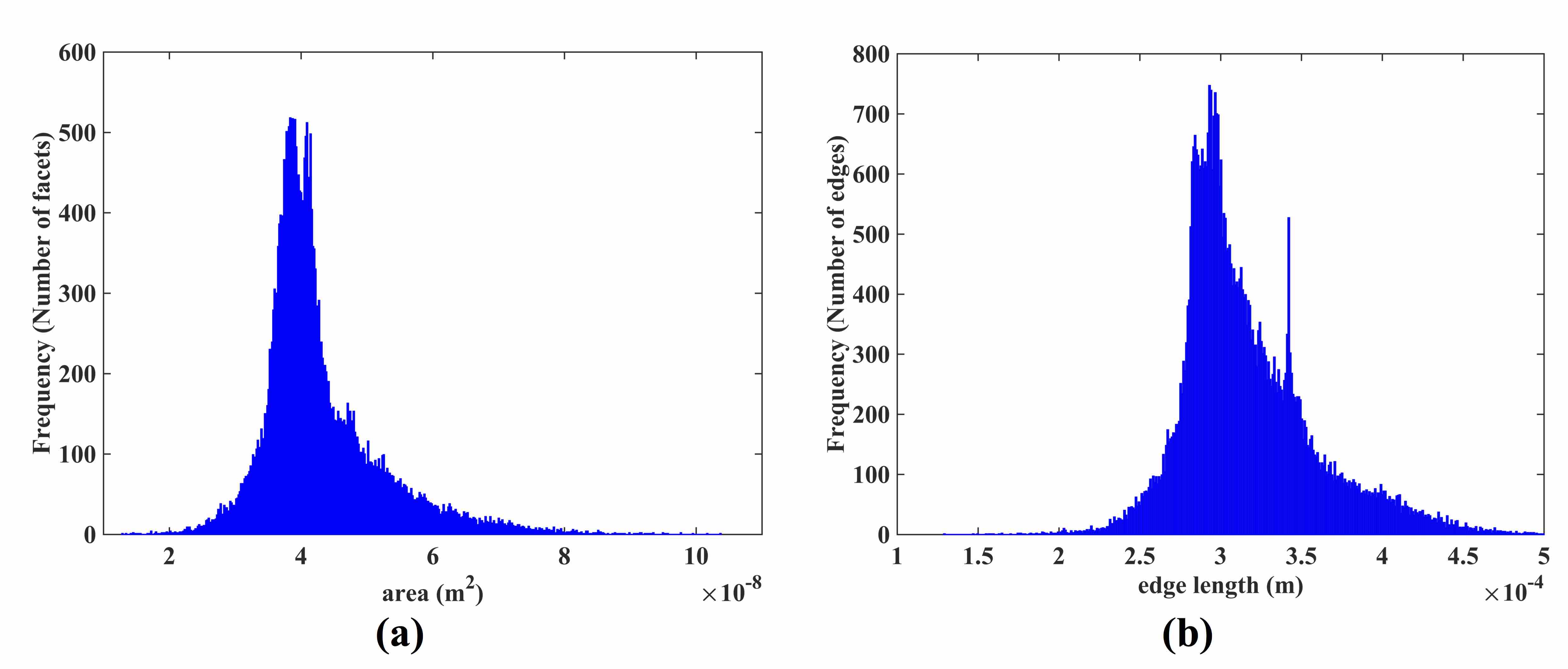
Figure 6: U-bend flow problem (Fig.5). Histogram plot for the (a) edge length and (b) area of the immersed boundary facets.

Table 3: U-bend flow probblem (Fig.5). Tetrahedral mesh resolution, number of Eulerian nodes, number of tetrahedral linear elements, and number of Lagrangian points for the successively denser grids.

$h$ (m)	Eulerian	Tetrahedral	Lagrangian	Surface
	nodes	elements	points	facets
$4\times 10^{-4}$	10,227	59,275	4,410	8,938
$2\times 10^{-4}$	71,589	414,928	16,760	33,516
$1\times 10^{-4}$	456,505	2,693,729	63,082	125,848

We use successively denser tetrahedral meshes to obtain a mesh independent numerical solution. The meshes used are listed in Table 3. We use a parabolic velocity profile ($u_{z}(r)=U_{\max}\left(1-\left(\frac{r}{R}\right)^{2}\right)$, $U_{\max}=0.122625~{}\mathrm{m/s}$) at the inlet (red circle in Fig. 5a), while at the outlet (green circle in Fig. 5a) we apply zero pressure $\left(p=0\right)$. At the remaining boundaries (shown in yellow in Fig. 5a) of the flow domain, we set no-slip boundary conditions. The (rectangular) flow domain has rigid walls (yellow faces in Fig. 5a) with no-slip boundary conditions, an inlet (red circle in Fig. 5a), where the fluid enters, and an outlet (green circle in Fig. 5a), where the fluid exits. The numerical solutions obtained using the the three meshes described in Table 3, were projected/interpolated on a body-fitted mesh consisting of 808,984 linear tetrahedral elements and 143,406 nodes.

Fig. 7a shows the axial velocity computed with the proposed method using successively denser meshes listed in Table 3. Fig. 7b shows a comparison of the axial velocity computed using the IB method, and the experimental data (red dots) at the tube outlet. The axial velocity is computed on the center plane at the start of the outlet extension (see Fig. 4a), where in excellent agreement between the velocity predicted using the proposed IB method and experimental results is observed. The numerical results obtained using the linear ($P_{1}/P_{1}$) elements are also in good agreement with the experimental data, highlighting the accuracy of the proposed method.

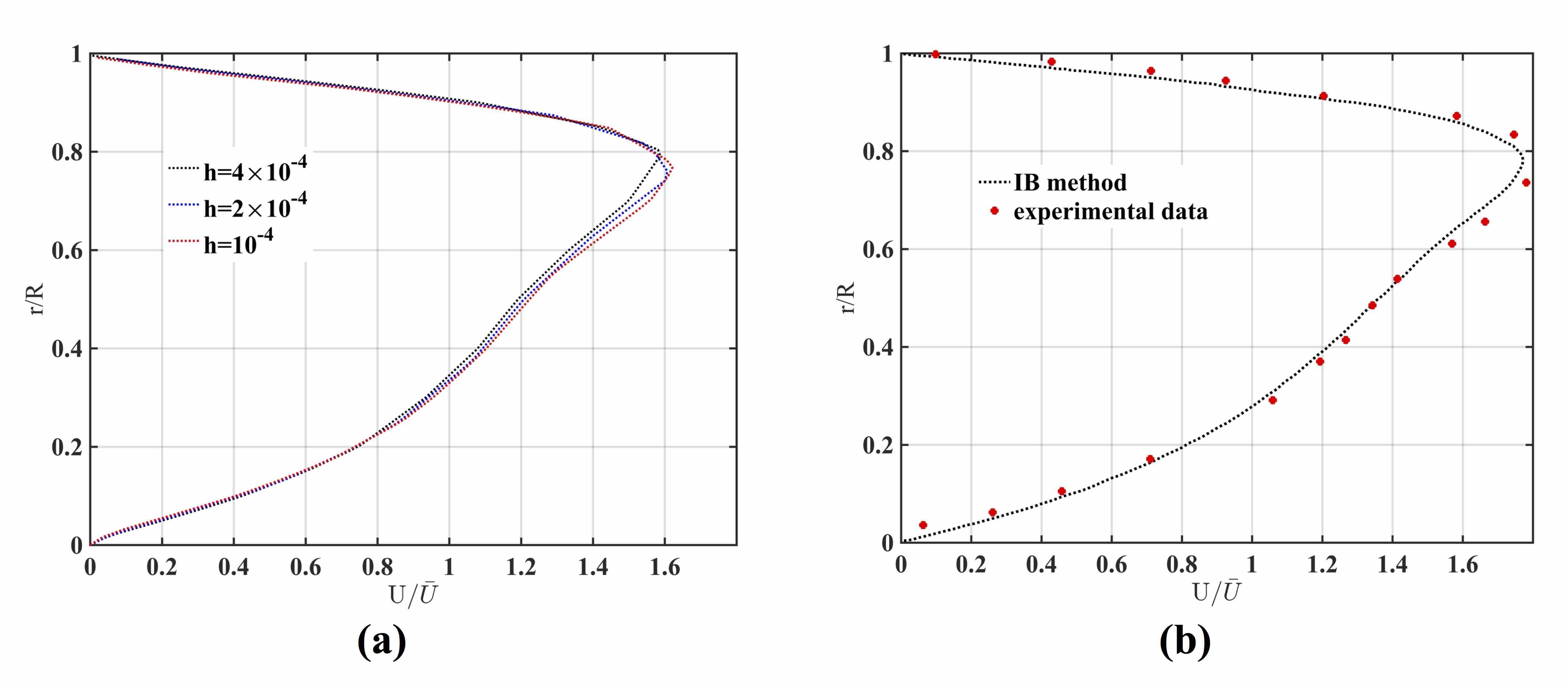
Figure 7: (a) Axial velocity computed with the proposed IB method using successively denser meshes described in Table 3 with $h$ being the mesh resolution close to the immersed boundary, and (b) axial velocity computed with the proposed IB method (dashed line) compared against the experimental data (red dots) at the tube outlet for the U-bend flow problem.

4 Numerical examples: blood flow simulations

In this section, we demonstrate the accuracy and robustness of the proposed scheme through blood flow simulations in complex vascular geometries. In the first flow problem, we simulate blood flow in coronary artery bifurcation (Fig. 8), while in the second we consider blood flow in the ascending aorta (Fig. 11). Finally, we consider the flow in the ascending and descending aorta (Fig. 14).

The flow problems considered demonstrate the applicability of the proposed method for internal flow simulations. Internal flow cases, are practically out of reach for all IB methods. The computational cost of having a tetrahedral mesh (uniform or locally refined) to discretize the flow domain is high, since only a small percentage of the total number of mesh elements, falls into the domain of interest [4]. The proposed IB method allows for cropping the tetrahedral mesh (see example 4.3) that covers the complex (vascular) geometry, and at the same time increases the percentage of elements that are located inside the flow domain of interest. In all flow cases considered, we use a locally refined mesh, in the vicinity and inside the Lagrangian points. We demonstrate the accuracy of the proposed IB method, by comparing the numerical findings with those computed using a body-fitted mesh FE flow solver. Local refinement is an automated procedure implemented using FEniCS built-in functions (Plaza algorithm [32]).

4.1 Flow in an coronary artery bifurcation

In the first example, we simulate the blood flow in a coronary artery (CA) bifurcation (shown in Fig. 8). The immersed boundary (coronary artery) is embedded into a box with dimensions $-0.0052\ m\leq x\leq 0.01\ m$, $-0.006\ m\leq y\leq 0.006\ m$ and $0\ m\leq z\leq 0.0296\ m$. The inlet and two outlets of the CA geometry were extruded to ensure that the flow is fully developed.

Table 4: Mesh resolution close to the immersed object, number of tetrahedral linear elements, mesh points, and number of Lagrangian points for the successively denser grids considered for the flow in the coronary artery bifurcation.

$h$ (m)	Eulerian	Tetrahedral	Surface	Lagrangian
	nodes	elements	facets	points
$4\times 10^{-4}$	18,364	117,864	3,689	1,770
$2\times 10^{-4}$	108,897	627,040	7,822	3,913
$1\times 10^{-4}$	618,565	3,641,633	14,894	7,449

We discretize the flow domain using tetrahedral elements. The box domain is discretized with a high quality tetrahedral mesh, generated using a uniform Cartesian grid (to generate the mesh we used the FEniCS build-in function BoxMesh). The tetrahedral mesh is locally refined in the vicinity and inside the immersed boundary (Figs. 8c-d). We use successively denser meshes to obtain a mesh independent numerical solution. The meshes used are listed in Table 4. The numerical results on the two finest meshes (for 627,040 and 3,641,633) are indistinguishable. Mesh generation is a straightforward and automated. The locally refined mesh with 3,641,633 elements is generated in less than 60 s (using a laptop computer with 2.7 GHz i7 quad-core processor and 16 GB internal memory), using the refine function in FEniCS. We define the mesh resolution close to the immersed object and in the interior based on the mean value of the surface elements area (see Section 3.2). The majority (85%) of the elements are located inside the immersed boundary (coronary artery).

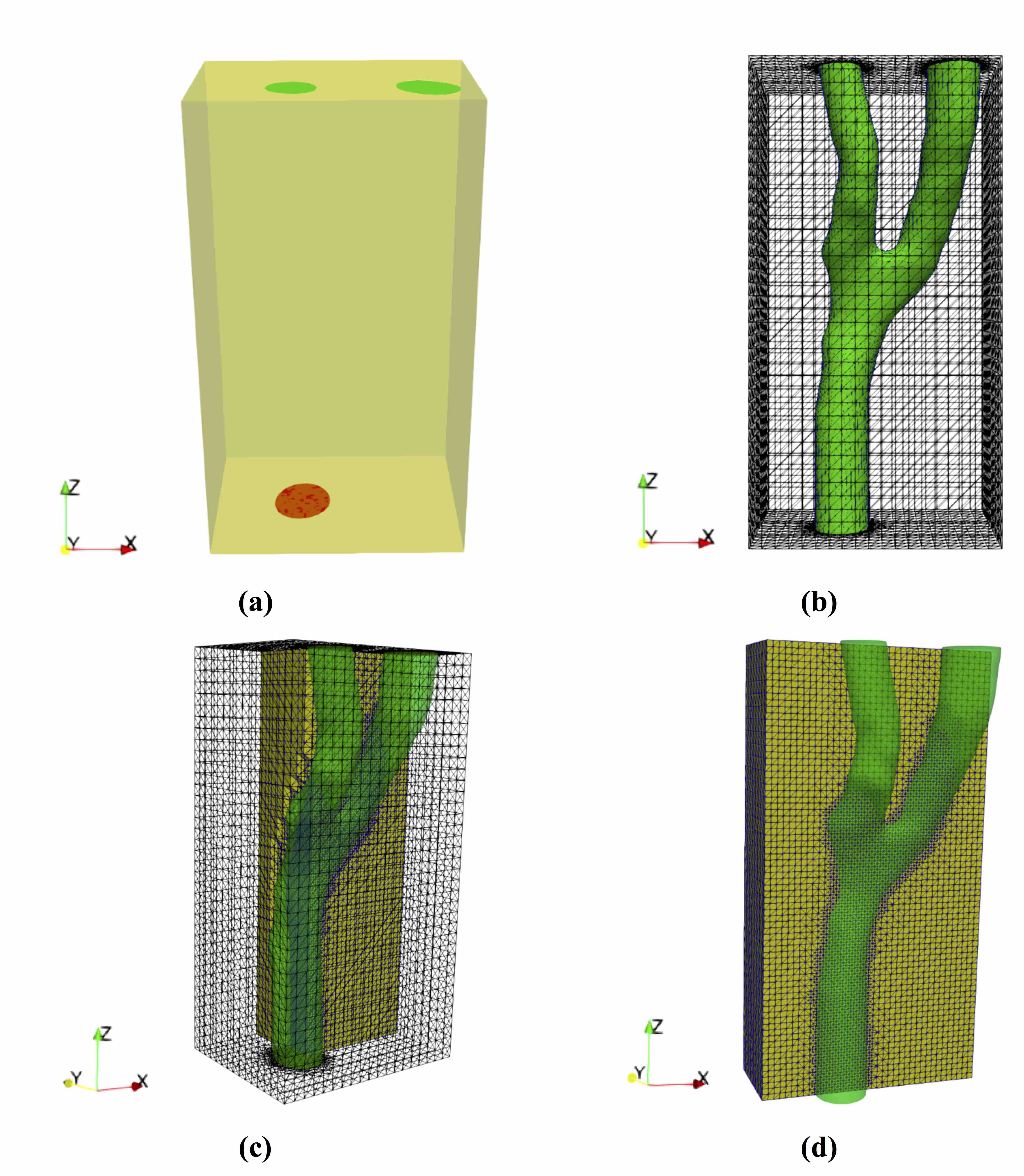
Figure 8: Flow domain for the coronary artery bifurcation example, with inlet (circle in red color), outlet (circle in green color) and walls (yellow color) boundaries; (b) wireframe of the tetrahedral mesh and the coronary artery immersed boundary (Lagrangian points); (c) tetrahedral mesh refined close and inside the immersed boundary, and (d) vertical cross-section of the tetrahedral mesh.

We set the total time for the simulation to $T=0.8$ s (one cardiac cycle), and the time step to $dt=5\times 10^{-4}$ s. At the inlet ((red area located at the bottom surface in Fig.(8a)) we apply the pulsatile velocity waveform shown in Fig. 9 (we use a parabolic velocity profile since the Womersley number is small), and zero pressure boundary conditions at the two outlets (green area on the top surface in Fig.(8a)). At the remaining walls (yellow surface in Fig.(8a)), we apply no-slip boundary conditions. We employ the Newtonian model for blood flow, with dynamic viscosity of $\mu=0.00345\ Pa\cdot s$ and density of $\rho=1,056\ \frac{\text{kg}}{m^{3}}$.

Figure 9: Pulsatile velocity waveform imposed at the inlet for the coronary artery bifurcation flow example.

To demonstrate the accuracy of our IB method, we compare the results obtained using this method with those for the body-fitted mesh. The body-fitted mesh consists of 154,681 nodes and 860,818 linear tetrahedral elements $\left(P_{1}/P_{1}\right)$. Table 5, lists the normalized root mean square error (NRMSE) $L_{\text{NRMSE}}=\frac{1}{N}\sqrt{\sum_{i=1}^{N}\left(u_{i}^{\text{IB}}-u_{i}^{\text{body\ fitted}}\right)^{2}}$ error norms at different time instances.

Table 5: $L_{2}$ error norm of the immersed boundary method numerical results against those computed using the body-fitted FE method at different time instances for the coronary artery bifurcation flow example.

$L_{2}$ (%)	$t=0.1$	$t=0.2$	$t=0.3$	$t=0.4$	$t=0.5$	$t=0.6$	$t=0.7$	$t=0.8$
$u_{x}$	1.53	1.38	2.03	1.94	1.94	1.88	1.84	1.74
$u_{y}$	2.32	3.17	3.34	3.27	3.28	3.23	3.16	2.78
$u_{z}$	3.34	3.82	4.57	4.42	4.44	4.37	4.06	3.84

The results obtained using our IB method and body fitted mesh reported in Table 5 are for practical purposes indistinguishable as in the bioengineering applications. The differences of under 5$\%$ would be overwhelmed by the biomechanical properties uncertainties. The decisive advantage of our method is the easiness of patient-specific computational grid generation with practically no increase in the computational cost. The only computational overhead of our IB method in comparison to the approach relying on a body fitted mesh is due to the numerical solution of the linear system given by Eq.(21). For the computation of flow in coronary artery bifurcation conducted here (Figure 8), this overhead was negligible — less than 1$\%$ of the total computation time. Fig. 10 shows the streamlines in the coronary artery bifurcation at time $t=0.14$ (diastole) and $0.25$ sec (peak systole).

Figure 10: Streamlines (left), pressure (middle) and wall shear stress (WSS) magnitude (Pa) (right) at (a) peak systole pressure and (b) diastolic minimum for the coronary artery bifurcation flow example.

4.2 Blood flow in the ascending aorta

In the second example, we simulate blood flow in the ascending aorta (the brachiocephalic, left common carotid, and left subclavian arteries are included in the model) shown in Fig. 11. The immersed boundary (ascending aorta) is embedded within a box (Fig. 11a) with dimensions $-0.037\ m\leq x\leq 0.035\ m$, $-0.08\ m\leq y\leq 0.04\ m$ and $0\ m\leq z\leq 0.12\ m$. The box domain is discretized with a high quality tetrahedral mesh, generated using a uniform Cartesian grid (to generate the mesh we used the FEniCS build-in function BoxMesh). The tetrahedral mesh is locally refined in the vicinity and inside the immersed boundary as shown in Fig.11c-d. We use successively denser meshes, indicated in Table 6, to obtain a mesh independent numerical solution. The numerical results on the two finest meshes (for 1,410,846 and 2,557,306) are indistinguishable. We refine the tetrahedral mesh close to the Lagrangian points and in the interior of the immersed boundary. As described in Section 2.5, the mesh resolution close to the immersed boundary (Lagrangian points) is based on on the mean area of the facets on the immersed object. Mesh generation and local refinement on the rectangular domain is a straightforward and efficient procedure. It took less than 30 s to generate the finest grid (information about this grid in the third row of Table 6) using a laptop computer with i7 quad-core processor with 16 GB internal memory.

Figure 11: (a) Flow domain for the ascending aorta flow example, with inlet (circle in red color), outlets (circle in green color) and walls (yellow color) boundaries; (b) wireframe of the tetrahedral mesh and the immersed boundary (ascending aorta); (c) horizontal cross-section of the tetrahedral mesh, and (d) vertical and horizontal cross-sections of the tetrahedral mesh.

Table 6: Mesh resolution close to the immersed object, number of tetrahedral mesh vertices, and number of Lagrangian points for the successively denser grids considered for the flow in the ascending aorta.

$h$ (m)	Eulerian	Tetrahedral	Surface	Lagrangian
	nodes	elements	facets	points
$1.5\times 10^{-3}$	61,930	355,296	7,410	3,584
$7.5\times 10^{-4}$	241,483	1,410,846	15,153	7,641
$3.75\times 10^{-4}$	439,126	2,557,306	31,684	15,938

We set the total time for the simulation to $T=0.8$ s (one cardiac cycle), and the time step $dt=5\times 10^{-4}$ s. At the inlet (red area in Fig. 11a) we apply the pressure waveform shown in Fig. 12, zero pressure boundary conditions at the two outlets (green area in Fig. 11a), and no-slip boundary conditions at the remaining walls (yellow surface in Fig. 11a). We employ the Newtonian model for blood flow, with dynamic viscosity of $\mu=0.00345\ \mathrm{Pa\,s}$ and density of $\rho=1,056\ \mathrm{kg/m^{3}}$. We use the diameter $D$ and the maximum velocity $U_{m}$ as the characteristic length and velocity to calculate the Reynolds number.

Figure 12: Pressure waveform used in the ascending aorta flow example.

To compare the flow velocity predicted using our IB method with the results from body fitted mesh, we interpolate our IB solution on a body fitted mesh consisting of 92,786 nodes and 504,628 linear tetrahedral elements. The comparison done at the time instances (every 0.1 s interval) indicated that the normalized root mean square error (NRMSE) of less than 5$\%$ for the three velocity components. We conducted also qualitative comparison of the predicted streamlines, pressure contours, and wall shear stress (WSS) contours at the time instances of $t=0.2$ and $t=0.6$ (Fig. 13). No visually distinguishable differences between the results obtained using our IB method and approach using body fitted mesh can be found in Fig. 13. (every 0.1 sec) the IB numerical solution with the numerical results obtained using the body-fitted mesh. The normalized root mean square error (NRMSE) $L_{\text{NRMSE}}$ for the three velocity components is less than 5%.

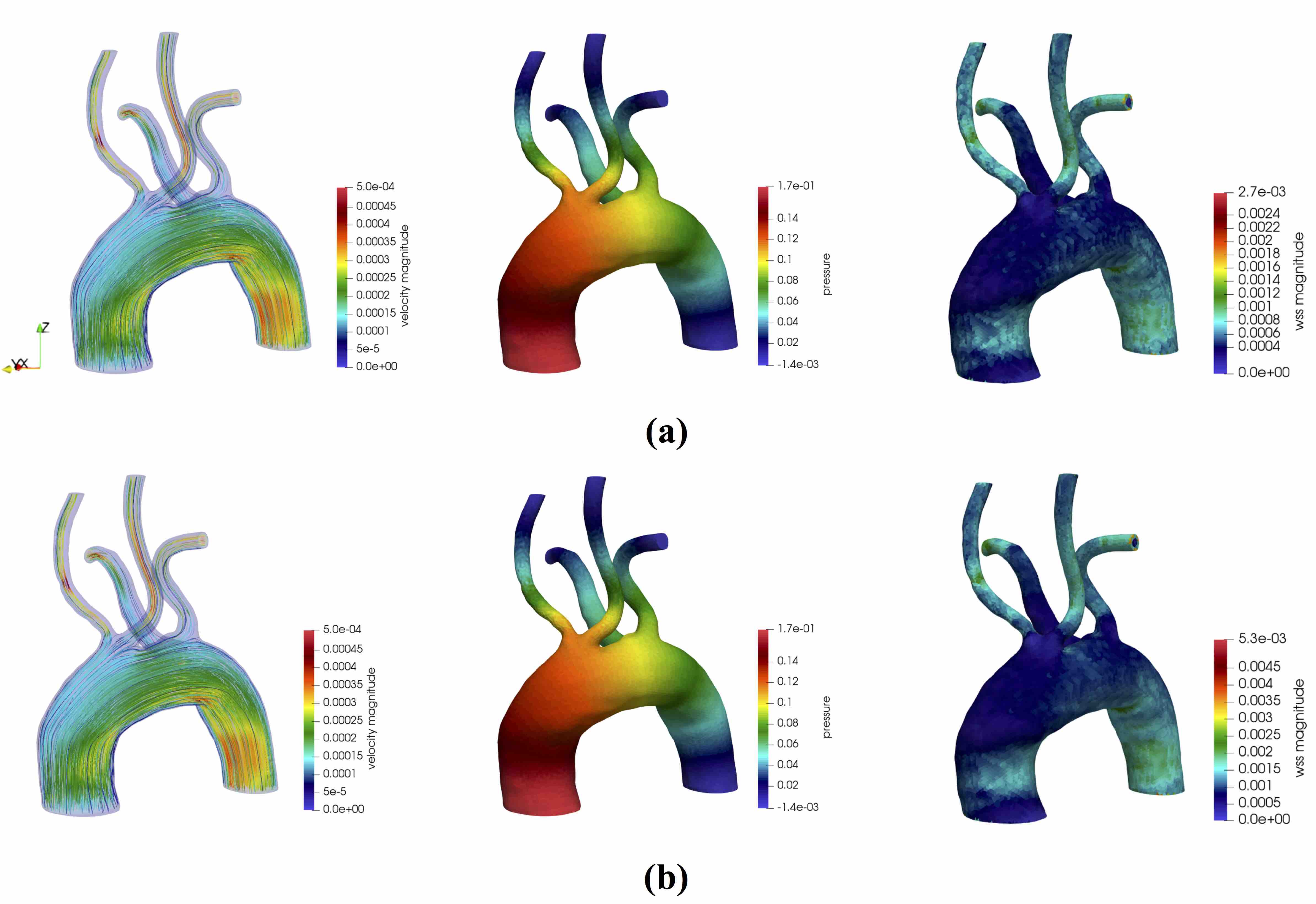
Figure 13: Streamlines (left), pressure (middle) and wall shear stress (WSS) magnitude (Pa) (right) contour plot at time (a) $t=0.2$ s and (b) $t=0.6$ s for the ascending aorta flow example.

Fig. 13 shows the streamlines (left), pressure (middle) and wall shear stress (WSS) magnitude (right) contours at different time instances $t=0.2$ and $t=0.6$. The results were obtained using the mesh with 1,410,846 tetrahedral elements.

4.3 Blood flow in the ascending and descending aorta

As the final example, we consider blood flow in the ascending and descending aorta. This example differs from the previous one (blood flow in the ascending aorta) by the number of outlets considered (the brachiocephalic, left common carotid, and left subclavian arteries were removed).

This flow example is more challenging because the inlet of the immersed object is located in the interior of the box flow domain and not on the boundary (Fig. 14a). Therefore, we crop the rectangular domain such that the inlet of the immersed object (red circle in Fig. 14a) is on the boundary of the flow domain (yellow color in Fig. 14a) and the boundary conditions can be easily applied.

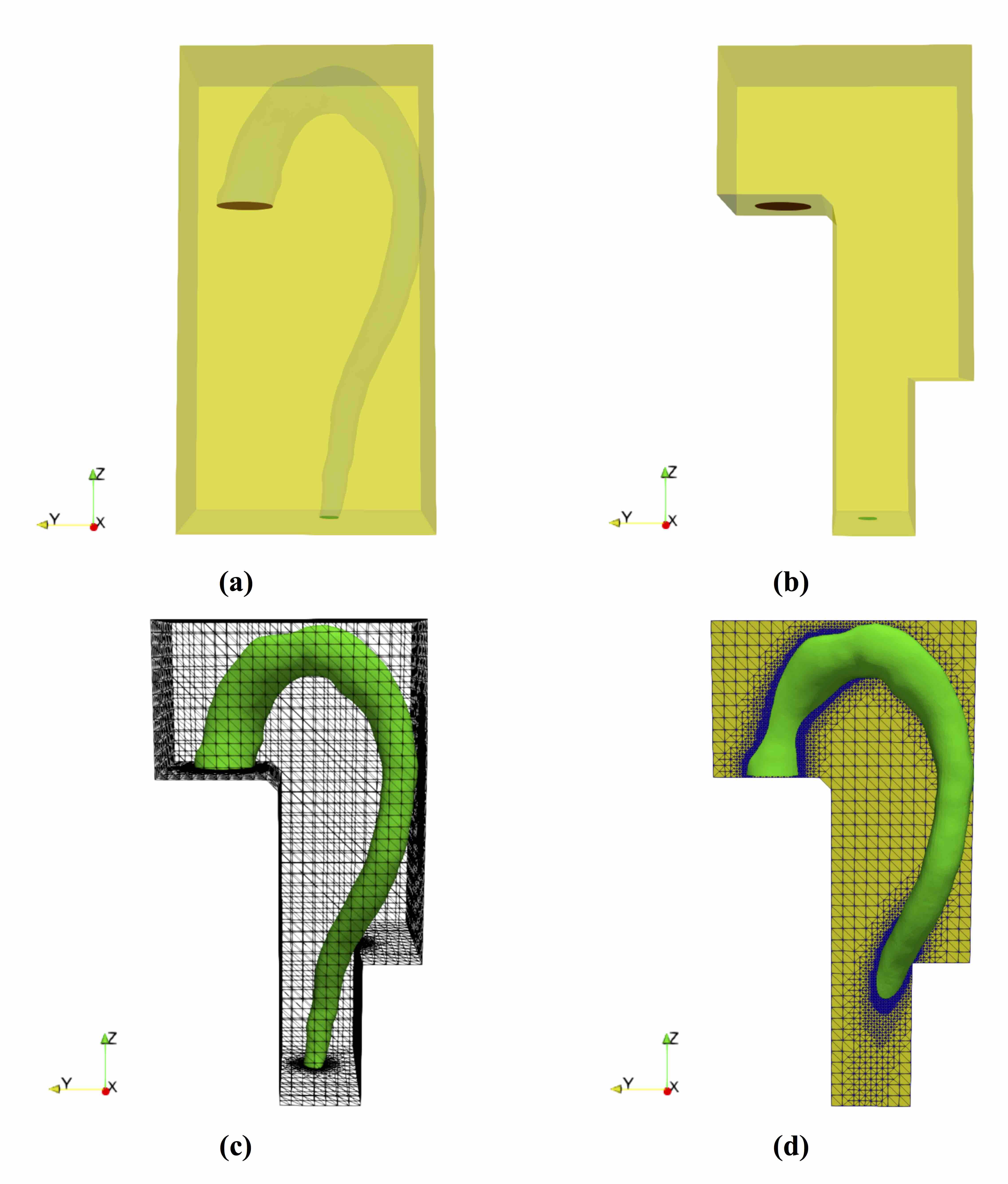
Figure 14: (a) Flow domain for the ascending and descending aorta flow example, with inlet (circle in red color), outlets (circle in green color) and walls (green color) boundaries; (b) cropped flow domain; (c) wireframe of the tetrahedral mesh and the immersed boundary (ascending and descending aorta) and, (d) horizontal cross-section of the tetrahedral mesh.

The immersed boundary (aorta) is embedded into a box domain (Fig. 14a) with dimensions $-0.042\ m\leq x\leq 0.0252\ m$, $-0.0806\ m\leq y\leq 0.025\ m$ and $-0.14\ m\leq z\leq 0.0616\ m$. The box domain is discretized with a high quality tetrahedral mesh, generated using a uniform Cartesian grid (to generate the mesh we used the FEniCS build-in function BoxMesh). The tetrahedral mesh is cropped and elements are removed (the cropped domain is shown in Fig. 14b). Finally, the cropped tetrahedral mesh is locally refined in the vicinity and inside the immersed boundary (Fig. 14d).

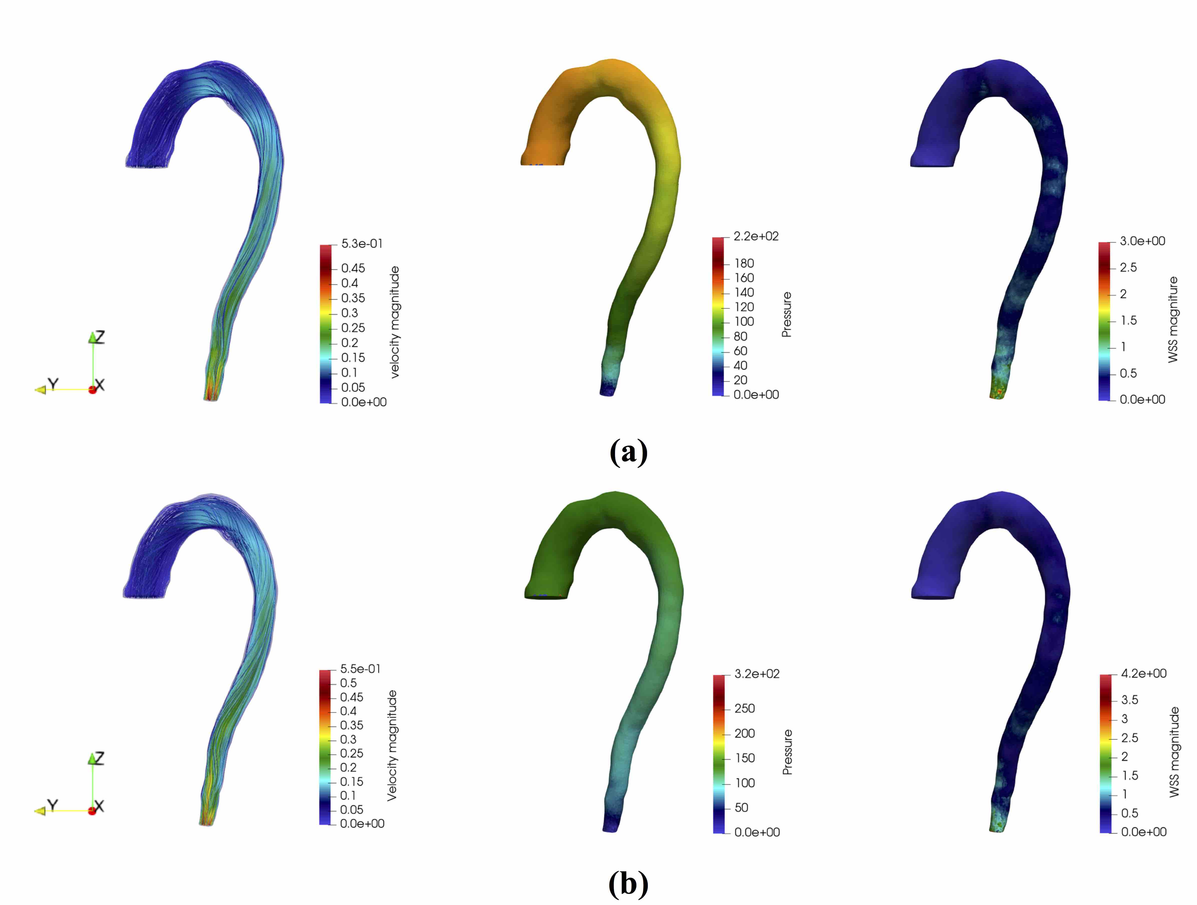
Figure 15: Streamlines (left), pressure (middle) and wall shear stress (WSS) magnitude (Pa) (right) contour plot at time (a) $t=0.2$ s and (b) $t=0.6$ s for the ascending and descending aorta flow example.

We use successively denser meshes to obtain a mesh independent numerical solution. A mesh of 417,227 nodes and 2,409,460 linear tetrahedral elements (approx. 85% of the elements are located inside the immersed boundary) ensures a mesh independent numerical solution. We apply a uniform velocity profile $\overline{U}$ (plug flow) at the inlet (in red color Fig. 14a). We apply zero pressure boundary conditions at the outlet, and no-slip boundary conditions in the remaining boundaries. We employ the Newtonian model for blood flow, with dynamic viscosity of $\mu=0.00345\ \mathrm{Pa\cdot s}$ and density of $\rho=1,056\ \mathrm{kg/m^{3}}$. The diameter $D$ at the inlet, and the velocity at the inlet $\overline{U}$, are used as the characteristic length and velocity to define the Reynolds number. For the inlet velocity value used in our simulations, the Reynolds number is $\mathrm{Re}=310$ for the present geometry.

Fig. 15 shows the streamlines (left), pressure (middle) and wall shear stress (WSS) magnitude (right) contours at different time instances $t=0.2$ and $t=0.6$.

5 Conclusions

In this work, we present an immersed boundary method for internal flows, showing blood flow application. The proposed scheme combines the finite element (FE) method, which is used to numerically solve the Navier–Stokes equations, and the boundary condition enforced immersed boundary (BCE-IB) method to account for complex geometries.

The proposed method increases the computational efficiency of the IB method for internal flows, by reducing the number of unused mesh points through a sophisticated and efficient method for mesh refinement in the vicinity and inside the immersed boundary. This method facilitated generation of a computational mesh consisting of over three and half million elements (computation of flow in an aortic bifurcation — see Fig. 8) in less than 30 seconds on an off-the-shelf laptop with quad-core i7 processor and 16 GB of internal memory. This very promising results make it possible to regard our adaptive mesh refinement method as compatible with the time constraints of clinical workflow (no firm definition here by the times of on order of under 1 minute have been reported in the literature [33]). Furthermore, we introduced an efficient method to reduce (crop) the flow domain, in flow cases where the immersed boundary inlet(s) and outlet(s) do not coincide with the boundaries of the flow domain (tetrahedral mesh).

The proposed method utilizes an efficient and accurate finite element solver based on incremental pressure correction scheme (IPCS). All simulations in this study were conducted using an off-the-shelf laptop with quad-core i7 processor and 16 GB of internal memory. The accuracy of the proposed scheme has been successfully verified through comparison with an analytical solution for the Poiseuille flow in a cylinder with circular cross section. We further validated the accuracy of the proposed method by solving a flow case where experimental data are available. The applicability and efficiency of the proposed method has been demonstrated through the solution of flow examples with complex geometry.

References

- Peskin [1972] C. S. Peskin, Flow patterns around heart valves: A numerical method, Journal of Computational Physics 10 (1972) 252–271. doi:10.1016/0021-9991(72)90065-4.
- Anupindi et al. [2013] K. Anupindi, Y. Delorme, D. A. Shetty, S. H. Frankel, A novel multiblock immersed boundary method for large eddy simulation of complex arterial hemodynamics, Journal of Computational Physics 254 (2013) 200–218. doi:10.1016/j.jcp.2013.07.033.
- de Zélicourt et al. [2009] D. de Zélicourt, L. Ge, C. Wang, F. Sotiropoulos, A. Gilmanov, A. Yoganathan, Flow simulations in arbitrarily complex cardiovascular anatomies – An unstructured Cartesian grid approach, Computers & Fluids 38 (2009) 1749–1762. doi:10.1016/j.compfluid.2009.03.005.
- Zhu et al. [2019] C. Zhu, J.-H. Seo, R. Mittal, A graph-partitioned sharp-interface immersed boundary solver for efficient solution of internal flows, Journal of Computational Physics 386 (2019) 37–46. doi:10.1016/j.jcp.2019.01.038.
- Mittal and Iaccarino [2005] R. Mittal, G. Iaccarino, Immersed Boundary Methods, Annual Review of Fluid Mechanics 37 (2005) 239–261. doi:10.1146/annurev.fluid.37.061903.175743.
- Peskin [1977] C. S. Peskin, Numerical analysis of blood flow in the heart, Journal of Computational Physics 25 (1977) 220–252. doi:10.1016/0021-9991(77)90100-0.
- Goldstein et al. [1993] D. Goldstein, R. Handler, L. Sirovich, Modeling a No-Slip Flow Boundary with an External Force Field, Journal of Computational Physics 105 (1993) 354–366. doi:10.1006/jcph.1993.1081.
- Saiki and Biringen [1996] E. M. Saiki, S. Biringen, Numerical Simulation of a Cylinder in Uniform Flow: Application of a Virtual Boundary Method, Journal of Computational Physics 123 (1996) 450–465. doi:10.1006/jcph.1996.0036.
- Lai and Peskin [2000] M.-C. Lai, C. S. Peskin, An Immersed Boundary Method with Formal Second-Order Accuracy and Reduced Numerical Viscosity, Journal of Computational Physics 160 (2000) 705–719. doi:10.1006/jcph.2000.6483.
- Khadra et al. [2000] K. Khadra, P. Angot, S. Parneix, J.-P. Caltagirone, Fictitious domain approach for numerical modelling of Navier–Stokes equations, International Journal for Numerical Methods in Fluids 34 (2000) 651–684. doi:10.1002/1097-0363(20001230)34:8<651::AID-FLD61>3.0.CO;2-D.
- Su et al. [2007] S.-W. Su, M.-C. Lai, C.-A. Lin, An immersed boundary technique for simulating complex flows with rigid boundary, Computers & Fluids 36 (2007) 313–324. doi:10.1016/j.compfluid.2005.09.004.
- Glowinski et al. [1998] R. Glowinski, T. W. Pan, J. Périaux, Distributed Lagrange multiplier methods for incompressible viscous flow around moving rigid bodies, Computer Methods in Applied Mechanics and Engineering 151 (1998) 181–194. doi:10.1016/S0045-7825(97)00116-3.
- Lee and LeVeque [2003] L. Lee, R. J. LeVeque, An Immersed Interface Method for Incompressible Navier–Stokes Equations, SIAM Journal on Scientific Computing 25 (2003) 832–856. doi:10.1137/S1064827502414060.
- Taira and Colonius [2007] K. Taira, T. Colonius, The immersed boundary method: A projection approach, Journal of Computational Physics 225 (2007) 2118–2137. doi:10.1016/j.jcp.2007.03.005.
- Mohd-Yusof [1997] J. Mohd-Yusof, Combined immersed-boundary/B-spline methods for simulations of flow in complex geometries, Annual Research Briefs. NASA Ames Research Center (1997) 317–327. URL: https://web.stanford.edu/group/ctr/ResBriefs97/myusof.pdf.
- Fadlun et al. [2000] E. A. Fadlun, R. Verzicco, P. Orlandi, J. Mohd-Yusof, Combined Immersed-Boundary Finite-Difference Methods for Three-Dimensional Complex Flow Simulations, Journal of Computational Physics 161 (2000) 35–60. doi:10.1006/jcph.2000.6484.
- Balaras [2004] E. Balaras, Modeling complex boundaries using an external force field on fixed Cartesian grids in large-eddy simulations, Computers & Fluids 33 (2004) 375–404. doi:10.1016/S0045-7930(03)00058-6.
- Gilmanov et al. [2003] A. Gilmanov, F. Sotiropoulos, E. Balaras, A general reconstruction algorithm for simulating flows with complex 3D immersed boundaries on Cartesian grids, Journal of Computational Physics 191 (2003) 660–669. doi:10.1016/S0021-9991(03)00321-8.
- Zhang and Zheng [2007] N. Zhang, Z. C. Zheng, An improved direct-forcing immersed-boundary method for finite difference applications, Journal of Computational Physics 221 (2007) 250–268. doi:10.1016/j.jcp.2006.06.012.
- Choi et al. [2007] J.-I. Choi, R. C. Oberoi, J. R. Edwards, J. A. Rosati, An immersed boundary method for complex incompressible flows, Journal of Computational Physics 224 (2007) 757–784. doi:10.1016/j.jcp.2006.10.032.
- Ghommem et al. [2020] M. Ghommem, G. Bourantas, A. Wittek, K. Miller, M. R. Hajj, Hydrodynamic modeling and performance analysis of bio-inspired swimming, Ocean Engineering 197 (2020) 106897. doi:10.1016/j.oceaneng.2019.106897.
- Wu and Shu [2009] J. Wu, C. Shu, Implicit velocity correction-based immersed boundary-lattice Boltzmann method and its applications, Journal of Computational Physics 228 (2009) 1963–1979. doi:10.1016/j.jcp.2008.11.019.
- Goda [1979] K. Goda, A multistep technique with implicit difference schemes for calculating two- or three-dimensional cavity flows, Journal of Computational Physics 30 (1979) 76–95. doi:10.1016/0021-9991(79)90088-3.
- unk [2019] FEniCS Project, 2019. URL: https://fenicsproject.org.
- Chorin [1968] A. J. Chorin, Numerical solution of the Navier-Stokes equations, Mathematics of Computation 22 (1968) 745–762. doi:10.1090/S0025-5718-1968-0242392-2.
- Témam [1969] R. Témam, Sur l’approximation de la solution des équations de Navier-Stokes par la méthode des pas fractionnaires (I), Archive for Rational Mechanics and Analysis 32 (1969) 135–153. doi:10.1007/BF00247678.
- Uhlmann [2005] M. Uhlmann, An immersed boundary method with direct forcing for the simulation of particulate flows, Journal of Computational Physics 209 (2005) 448–476. doi:10.1016/j.jcp.2005.03.017.
- Kang and Hassan [2011] S. K. Kang, Y. A. Hassan, A comparative study of direct-forcing immersed boundary-lattice Boltzmann methods for stationary complex boundaries, International Journal for Numerical Methods in Fluids 66 (2011) 1132–1158. doi:10.1002/fld.2304.
- Lima E Silva et al. [2003] A. L. F. Lima E Silva, A. Silveira-Neto, J. J. R. Damasceno, Numerical simulation of two-dimensional flows over a circular cylinder using the immersed boundary method, Journal of Computational Physics 189 (2003) 351–370. doi:10.1016/S0021-9991(03)00214-6.
- Bourantas et al. [2016] G. C. Bourantas, B. L. Cheeseman, R. Ramaswamy, I. F. Sbalzarini, Using dc pse operator discretization in eulerian meshless collocation methods improves their robustness in complex geometries, Computers & Fluids 136 (2016) 285 – 300. doi:https://doi.org/10.1016/j.compfluid.2016.06.010.
- Van De Vosse et al. [1989] F. N. Van De Vosse, A. A. Van Steenhoven, A. Segal, J. D. Janssen, A finite element analysis of the steady laminar entrance flow in a 90° curved tube, International Journal for Numerical Methods in Fluids 9 (1989) 275–287. doi:10.1002/fld.1650090304.
- Plaza and Carey [2000] A. Plaza, G. Carey, Local refinement of simplicial grids based on the skeleton, Applied Numerical Mathematics 32 (2000) 195 – 218. doi:https://doi.org/10.1016/S0168-9274(99)00022-7.
- Wittek et al. [2010] A. Wittek, G. Joldes, M. Couton, S. K. Warfield, K. Miller, Patient-specific non-linear finite element modelling for predicting soft organ deformation in real-time; application to non-rigid neuroimage registration, Progress in Biophysics and Molecular Biology 103 (2010) 292 – 303. doi:https://doi.org/10.1016/j.pbiomolbio.2010.09.001, special Issue on Biomechanical Modelling of Soft Tissue Motion.