Abstract

Numerical modeling is used to investigate the dynamics of a polaron in a chain with small random Langevin-like perturbations which imitate the environmental temperature $T$ and under the influence of a constant electric field. In the semiclassical Holstein model the region of existence of polarons in the thermodynamic equilibrium state depends not only on temperature but also on the chain length. Therefore when we compute dynamics from initial polaron data, the mean displacement of the charge mass center differs for different-length chains at the same temperature. For a large radius polaron, it is shown numerically that the “mean polaron displacement” (which takes account only of the polaron peak and its position) behaves similarly for different-length chains during the time when the polaron persists. A similar slope of the polaron displacement enables one to find the polaron mean velocity and, by analogy with the charge mobility, assess the “polaron mobility”. The calculated values of the polaron mobility for $T\approx 0$ are close to the value at $T=0$, which is small but not zero. For the parameters corresponding to the small radius polaron, simulations of dynamics demonstrate switching mode between immobile polaron and delocalized state. The position of the new polaron is not related to the position of the previous one; charge transfer occurs in the delocalized state.

Keywords: Langevin thermostat, polaron mobility, small radius polaron, large radius polaron, homogeneous DNA.
2000 MSC: 34C60, 60J65

1 Introduction

Discrete nonlinear systems have appeared in the various fields of physics, chemistry and biology [1, 2, 3, 4, 5, 6, 7, 8, 9] and have attracted considerable attention recently. The problem of charge transfer in quasi-one-dimensional molecules, such as DNA or proteins, is of interest to biophysics. Due to its stability the polaron mechanism of charge transfer attracts attention of a great number of researchers. Presently it is believed that current carriers in DNA are polarons or solitons, see for example [2, 9, 10, 11] and references therein. The interest in the charge transfer mechanisms is also associated with the possibility of using DNA in molecular electronics [10, 11, 12].

Here we calculate the polaron properties in the semi-classical Holstein model, where chain of sites corresponds to the simplest representation of the DNA duplex as a sequence of nucleotide pairs. The polaron dynamics was studied earlier in the Holstein model for unperturbed chains in an external electric field both analytically (in a continuous medium) [13] and numerically [14, 15, 16, 17]. It was assumed that weak excitations of the chain (with energy much less than the characteristic energy equal to the depth of the polaron level) change the polaron properties only slightly.

However in the case when the chain is always affected by a random force (Langevin thermostat) weak excitations influence considerably the polaron characteristics. In the paper by Lomdahl and Kerr [18] direct numerical experiments demonstrated that Davydov soliton at physiological temperatures quickly decays and cannot transfer energy. For the soliton coupling energy of about 300 K, its disruption occurs at low temperature less than 10 K. Subsequent numerical experiments and analytical estimate of different authors [19, 20, 21, 22, 23] confirmed the conclusion that at physiological temperatures in biomacromolecules polarons decay and a charge is delocalized.

Earlier for a Holstein model a charge mobility $\mu$ was calculated in the range of “high” temperatures $T$ [24], when a charge is delocalized, and the temperature dependence of the mobility is estimated [25]. The dependence $\mu(T)\sim T^{-2.3}$ [25] means a growth of the mobility as the temperature decreases. This estimation is applicable in the range of high temperatures. It is assumed that in the range of low temperatures a charge forms a polaron state in a chain with far less mobility [12, 26].

In an unperturbed chain (at $T=0$), the polaron dynamics does not depend on the chain length (if the chain is much longer than the polaron size, of course). E.g., under the action of an electric field with constant intensity, polarons move with the same velocity in the chains of different length. The results of modeling at $T\neq 0$ demonstrate [27, 28] that in the thermodynamic equilibrium state (TDE) the existence of polaron depends not only on the thermostat temperature $T$, but also on the length of the chain $N$, i.e. on the thermal energy of the chain $NT$. Hence, at the same temperature, in the TDE in short chains a polaron does not decay while in long chains (heat energy of the chain grows with $N$) a charge is delocalized. In the region of polaron existence, at the same temperature in the TDE the mean characteristics, such as delocalization parameter and maximum probability of charge localization, depend on the chain length. Therefore in this region there are no stationary processes (similar to the root-mean-square deviation $\langle X^{2}(t)\rangle$ or mean displacement $\langle X(t)\rangle$ under the influence of an external electric field) which depend only on temperature.

Here we present the results of modeling the charge dynamics in different-length chains from the initial data “a polaron $+$ thermal fluctuations of the chain”. Numerical simulations enabled us to find some general dependencies at the same temperature and the same intensity of the external electric field at the first stage when a polaron has not yet disrupted. Small temperature region is considered where in the TDE a charge forms a polaron in relatively long chains. The results obtained are partly in a “nonphysical region”: for temperatures below Debye temperature $\Theta$, a classical description of the sites motion is inapplicable [18]. For this reason the simulation results are of qualitative interest. Two cases are considered – small radius polaron (SRP) with the parameters partly corresponding to homogeneous adenine DNA chains and a large radius polaron (LRP) with the parameters of thymine fragments.

Presently, there are many papers devoted to modeling the motion of a charged particle in various-type molecular chains (e.g., [23, 29, 30, 31, 32, 33, 34, 35, 36], also reviews [11, 37] and references therein). In some papers polaron is considered (according to the physical definition of SRP) for parameter values at which the polaron is localized at several sites. Here for SRP we consider the case when the charge is localized at one site with probability of almost 1, and LRP is localized in the region of about 15 sites. Also other works do not discuss the effect of chain length on the polaron state at a given temperature, most likely because with “physically significant” parameter values such effect is hard to notice on the computation time intervals. In our simulation we chose the adapted values of the parameters that speed up the system s movement to the TDE, and we suggest that not only the mean values in the TDE are the same for two systems with the same ratio of parameters [28], but the processes of reaching the TDE state from the same initial polaron state will be qualitatively similar.

The paper is arranged as follows. In Section 2 we describe the model and motion equations, in Section 3 the model parameters and the initial data are given, in Section 4 we describe the results of modeling the SRP, in Section 5 the results of LRP calculations are given and (by analogy with the charge mobility) estimation of the polaron mobility is made.

2 Model

The model is based on the Holstein Hamiltonian for discrete chain of sites [38]. In the semiclassical approximation, choosing the wave function $\Psi$ in the form $\Psi=\sum_{n=1}^{N}b_{n}|n\rangle$, where $b_{n}$ is the amplitude of the probability of the charge (electron or hole) occurrence at the $n$-th site ($n=1,{\ldots},N$, $N$ is the chain length) the averaged Hamiltonian has the form:

$$\langle\Psi|\hat{H}|\Psi\rangle =\sum_{m,n}\nu_{nm}b_{m}b_{n}^{*}+\frac{1}{2}\sum_{n}M\dot{\tilde{u}}_{n}^{2}+$$

$${}+\frac{1}{2}\sum_{n}K\tilde{u}_{n}^{2}+\sum_{n}\alpha^{\prime}\tilde{u}_{n}b_{n}b_{n}^{*}+\sum_{n}e\tilde{V}anb_{n}b_{n}^{*}.$$ (1)

Here $\nu_{mn}$ ($m\neq n$) are matrix elements of the charge transition between $m$-th and $n$-th sites (depending on overlapping integrals), $\nu_{nn}$ is the electron energy on the $n$-th site. We consider the nearest neighbour approximation: $\nu_{mn}=0$, if $m\neq n\pm 1$. The charge energy at the sites depends linearly on the sites displacements $\tilde{u}_{n}$, $\alpha^{\prime}$ is the coupling constant, $M$ is the $n$-th site’s effective mass, $K$ is the elastic constant. We deal with homogenous chains and choose $\nu_{nn}=0$. The last term in (1) takes account of the constant external field of intensity $\tilde{V}$, $e$ is the electron charge, $a$ is the distance between neighbouring sites.

Motion equations for Hamiltonian (1) have the form:

$$i\hbar\frac{db_{n}}{d\tilde{t}} =\nu_{n,n-1}b_{n-1}+\nu_{n,n}b_{n}+\nu_{n,n+1}b_{n+1}+\alpha^{\prime}\tilde{u}_{n}b_{n}+ean\tilde{V}b_{n},$$ (2)

$$M\frac{d^{2}\tilde{u}_{n}}{d\tilde{t}^{2}} =-K\tilde{u}_{n}-\alpha^{\prime}|b_{n}|^{2}-\tilde{\gamma}\frac{d\tilde{u}_{n}}{d\tilde{t}}+\tilde{A}_{n}(\tilde{t}).$$ (3)

To model a thermostat, subsystem (3) involves the terms with friction ($\tilde{\gamma}$ is the friction coefficient) and the random force $\tilde{A}_{n}(\tilde{t})$ such that $\langle\tilde{A}_{n}(\tilde{t})\rangle=0$, $\langle\tilde{A}_{n}(\tilde{t})\tilde{A}_{m}(\tilde{t}+\tilde{s})\rangle=2k_{B}\tilde{T}\tilde{\gamma}\delta_{nm}\delta(\tilde{s})$ ($\tilde{T}$ is the temperature [K], $k_{B}$ is Boltzmann constant). This way of imitating the environmental temperature with the use of Langevin equations (3) is well known [18, 39].

Motion equations (2),(3) for homogeneous chain after nondimensionalization have the form

$$i\frac{db_{n}}{dt} =\eta(b_{n-1}+b_{n+1})+\chi u_{n}b_{n}+nVb_{n},$$ (4)

$$\frac{d^{2}u_{n}}{dt^{2}} =-\omega^{2}u_{n}-\chi|b_{n}|^{2}-\gamma\frac{du_{n}}{dt}+\xi Z_{n}(t).$$ (5)

The relation between dimension and dimensionless parameters is as follows. The matrix elements $\eta=\nu_{n,n\pm 1}\tau/\hbar$, the frequency of sites oscillation $\omega=\sqrt{\tau^{2}K/M}$ ($\tau$ is the characteristic time, $\tilde{t}=\tau t$). The coupling constant is $\chi=\alpha^{\prime}\sqrt{\tau^{3}/\hbar M}$; $\gamma=\tau\tilde{\gamma}/M$; $V=ea\tilde{V}\tau/\hbar$. $Z_{n}(t)$ is random term with the properties

$$\langle Z_{n}(t)\rangle=0,\quad\langle Z_{n}(t)Z_{m}(t+t^{\prime})\rangle=\delta_{mn}\delta(t^{\prime}),$$

$$\xi=\sqrt{\frac{2k_{B}T^{*}\tau}{\hbar}}\sqrt{\gamma T},\qquad$$ (6)

where the dimensionless temperature is $T=\tilde{T}/T^{*}$, $T^{*}$ is characteristic value. Though the chain is homogeneous, under the electric field with intensity $V$ the electron energy on the $n$-th site is $nV$.

For $T=0$, $V=0$ the state with the lowest energy will be a polaron [26, 38]; in this case the velocities of the sites $\dot{u}_{n}=0$, and displacements are:

$$u_{n}=-\frac{\chi}{\omega^{2}}|b_{n}|^{2}.$$ (7)

Theoretical estimates of total energy for Hamiltonian (1) in the case of SRP when $\eta$ is small and a charge is localized at one ($n$-th) site with the probability $p_{n}=|b_{n}|^{2}\approx 1$

$$E\approx-\frac{1}{2}\frac{\chi^{2}}{\omega^{2}},$$ (8)

and in the case of LRP when the probabilities change only slightly at neighboring sites [38]

$$E\approx 2\eta+\frac{1}{48}\frac{\chi^{4}}{\eta\omega^{4}}$$ (9)

(here $\eta<0$).

3 Setting up a computational experiment

For a predetermined temperature of the thermostat $T$, we compute a set of realizations (trajectories of the system (4), (5) from different initial data and with different pseudo-random time-series) and calculate time dependencies averaged over realizations (“by ensemble”). We consider finite chains with free ends, i.e. initial value problem.

For the initial data we use polaron (the amplitudes of probability $b_{n}$ and displacements (7) corresponds to the lowest energy for $T=0$), Gaussian random variables are added to these displacements, and the velocities of the sites $\dot{u}_{n}$ are determined by Gaussian random variables with a relevant distribution.

The parameters of the model corresponding to nucleotide pairs [40, 41, 42] are: $M=10^{-21}$ g, terahertz frequency of the sites oscillations $\tilde{\omega}=10^{12}$ sec^-1 corresponds to rigidity of the hydrogen bonds $K\approx 0.062$ eV/Ų, the coupling constant $\alpha^{\prime}=0.13$ eV/Å. In the adenine chain polyA, for neighboring adenines, the matrix element of the transition between the sites is $\nu_{\mathrm{AA}}=0.030$ eV, and in the thymine fragment polyT $\nu_{\mathrm{TT}}=0.158$ eV. In dimensionless form in choosing the characteristic time $\tau=10^{-14}$ sec this corresponds to $\eta_{\mathrm{AA}}=0.456$, $\eta_{\mathrm{TT}}=2.4$, $\omega=0.01$, $\chi=0.02$ ($\chi/\omega=2$). The characteristic temperature value is $T^{*}=1$ K. In the polyA chains SRP is formed, for $T=0$ in the state with the lowest energy a charge is localized at one site with the probability of $p_{n}=|b_{n}|^{2}\approx 0.97$; in polyT chains LRP exists, a charge is localized in the region less than 20 sites with the maximum probability $\max_{n}p_{n}=p_{M}\approx 0.22$. Fig. 1 shows the probability distribution for polyA and polyT.

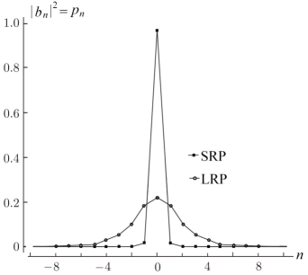
Figure 1: Polarons with parameter values for polyA (SRP) and polyT (LRP) at $T=0$.

The relations (8),(9) suggest that the system energy depends on the ratio $\chi/\omega$. It was shown [28] for homogeneous chains, that in the TDE the mean values depend not on the parameter values but on their ratios: in systems with the parameters

$$\{\eta,\chi,\omega\}\quad\text{and}\quad\{\eta,C\chi,C\omega\}\quad(C=const)$$ (10)

the averaged distribution of the probabilities, the total energy, the averaged polaron size $\langle R\rangle$ are similar. However the time to reach the TDE from the polaron initial state depends on the classical frequency of the system $\omega$.

In numerical simulations for the classical subsystem we mainly used adapted values of the parameters $\omega=0.5$, $\chi=1$ ($\chi/\omega=2$), for which the system quicker comes to the TDE. We suggest that a qualitative picture of polaron decaying is similar for different parameters in which the ratio $\chi/\omega$ holds; some test calculations do not contradict this assumption.

The possibility of polaron transfer for different intensities $V$ from 0 to 0.1 was investigated. The value $V=0.1$ for choosing DNA parameters corresponds to the intensity $\tilde{V}\approx 3\cdot 10^{7}$ V/m. This value is not very large in nanometer scale; thus, in experiments [43] the voltage up to 10 V was applied to the ends of 20-site DNA chain. The distance between the neighboring base pairs is $a\approx 0.34$ nm, i.e. $\tilde{V}\approx 3\cdot 10^{8}$ V/m.

In all the realizations at $t=0$ the polaron center was localized at one and the same site $n_{0}$. In the numerical experiment we calculate (and then for LRP we usually average over 50–100 realizations): the probabilities to find the charge at the $n$-th site $p_{n}(t)$, and the parameter of delocalization $R(t)$

$$R=\frac{1}{\sum_{1}^{N}|b_{n}|^{4}}=\frac{1}{\sum p_{n}^{2}}.$$ (11)

(In other papers [29, 30, 44, 32] $R(t)$ is also called participation number, localization length, degree of delocalization or measure of the locality of a polaron). This value correlate with charge distribution in the chain. If a charge is localized at one site, $p_{n}(t)\approx 1$, then $R(t)\approx 1$. If a charge is uniformly distributed over a $N$-site chain, $p_{n}=1/N$, then $R=N$. If the charge passes on to the delocalized state at $T\neq 0$, then in the TDE averaged over realizations $\langle R\rangle\approx N/2$ [27]. Value of $R$ may be associated with polaron radius. For $T=0$ in polyA chains (SRP) $R\approx 1.07$, in polyT chains (LRP) $R\approx 6.8$.

Also in the realization the probability maximum $p_{M}(t)=\max_{n}p_{n}(t)$ and $n_{M}(t)$ – the number of the site at which $p_{M}$ is localized – are calculated (similar method for soliton recognizing was proposed in [18]). For $V\neq 0$, we calculate the mean displacement of the charge center of mass

$$X(t)=\sum_{n}p_{n}(t)(n-n_{0}).$$ (12)

Knowing the dependencies $\langle X(t)\rangle$ for different $V$, we can estimate the charge velocity $v$ from the slope on a linear fragment (if any) and assess the charge mobility $\mu$:

$$v=\Delta X/\Delta t,\quad\mu=v/V$$ (13)

(theoretically, $\mu$ should be equal for different $V$ for region of the Ohm’s linear law). Similarly we calculate

$$X_{M}=p_{M}(n_{M}-n_{0})$$ (14)

(a certain analog of $X$, taking account of only the probability maximum) and keep track of the displacements $u_{M}(t)$ of the sites that have maximum probability. Besides in the “chain with window” where the fragment with the center $n_{M}$ is not considered (we usually took out $L=5$ sites on either side for SRP, i.e. 11 sites with the center $n_{M}$ for a SRP, and $L=10$ sites for LRP, i.e. 21 sites with the center $n_{M}$), we choose a site with the greatest in modulus displacement

$$u_{K}:|u_{K}|=\max_{|n-n_{M}|>L}|u_{n}|.$$ (15)

If a charge is in the polaron state, i.e. it is localized in a small region, then outside this region displacements are mainly determined by random fluctuations. This is an additional check up: if $|u_{K}|>|u_{M}|$, then we assume that there is not a polaron in the chain; if in this case $p_{M}$ is much larger than the mean probability $\langle p_{n}\rangle\approx 1/N$ in the chain, this may be a certain analog of a solectron (a charge was pulled into the well with the largest displacement) [45]; however, in simulations we did not observe such a situation.

Calculations of individual realizations for the values $\omega=0.5$, $\chi=1$ were performed by 2o2s1g-method [46] with forced normalization procedure. The system (4,5) has the first integral: the total probability of the charge occurrence in the chain $\Sigma=\sum_{n}p_{n}=\sum_{n}|b_{n}|^{2}$ must be equal to 1. The time intervals of computation can be very long. As result of numerical integration $\Sigma$ is not kept exactly. One of the ways that allows us to make computation intervals longer is forced normalization, when the variables $b_{n}$ will be “corrected” if $|\Sigma-1|>\varepsilon$: after the integration step we obtain values $b_{n}[old]$, calculate $\Sigma[old]$, and $b_{n}[new]=b_{n}[old]/(\Sigma[old])^{1/2}$, so $\Sigma[new]=1$. By test computations, for integration step $h=0.0005$ (or less) in the individual trajectory (with the same random seed and initial data) for $\varepsilon=10^{-4},10^{-5}$ and $10^{-6}$ the differences $|(u_{n})_{\varepsilon 1}-(u_{n})_{\varepsilon 2}|$ and $|(p_{n})_{\varepsilon 1}-(p_{n})_{\varepsilon 2}|$ is less then $10^{-6}$. Also we calculated the set of 50 realizations for $h=0.0002$ and compared the averaged values in the TDE with results for $h=0.0005$ ($\langle R\rangle$, $\langle p_{M}\rangle$, $\langle u_{M}\rangle$), and time intervals during which the system attains the TDE (see Fig. 2 below); these values for these steps are close. For “slower” values of the frequency (for example, $\omega=0.05$, $\chi=0.1$ or $\omega=0.01$, $\chi=0.02$) the trajectories were calculated using the combined scheme [47], where subsystem (4) is solved by a more accurate Runge–Kutta 4-order method, subsystem (5) with a random term in right-hand side – by the 2o2s1g method, and the interaction of the subsystems is taken into account in a special way. Using similar tests, the integration step $h=0.002$ and $\varepsilon=10^{-4}$ were chosen.

We considered different $N$ and $T$, for each pair $(N,T)$ the set of 50–100 realizations was calculated. When choosing $N$, $T$, we used the results [28]: for polyA fragments (SRP) the energy of the polaron decay is $NT_{crit}\approx 650$, and for polyT chains (LRP) $NT_{crit}\approx 380$.

Though the main results were obtained with adopted “accelerating” values of the parameters, we believe that the qualitative picture of the dynamics is similar in a wide range of the parameters for the systems (10). This assumption is confirmed by some test computations. For example, in Figs. 3 and 4 we plot the dynamics for 40-site chains with the parameters $\{\eta=0.456,\chi=1.,\omega=0.5\}$ and $\{\eta=0.456,\chi=0.2,\omega=0.1\}$ (SRP, $\eta$ value corresponds to polyA in quantum subsystem (4)), and in Fig. 12 – for LRP with different $\chi,\omega$ ($\eta=2.4$ correspond to polyT).

4 Results. Small Radius Polaron

For $V=0$ at small values $T$ polaron is immobile. In the TDE the maximum of the probability $p_{M}$ decreases as $T$ grows, however the polaron center $n_{M}$ does not change. Fig. 2 shows the $\langle R(t)\rangle$ curves (eq. (11)) for different $T$ in the chain of $N=40$ sites. For each $T$ 2 sets of 50 realizations were calculated: from the polaron initial data ($\langle R(t=0)\rangle\approx 1.07$) and from uniform distribution $b_{n}(t=0)=1/\sqrt{40}$ with random initial displacements $u_{n}$ and velocities $v_{n}$ from the Gauss distribution for given $T$ ($\langle R(t=0)\rangle=40$).

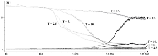
Figure 2: $\langle R(t)\rangle$ from the polaron initial data (black) and from uniform distribution $p_{n}(t=0)=1/N$ (gray). $N=40$, $\eta=0.456$, $\chi=1.$, $\omega=0.5$ ($\chi/\omega=2$), $\gamma=4\omega$. On the right, values of $T$ are indicated by arrows. Dotted line $R=1.07$ corresponds to polaron distribution $R(T=0)$.

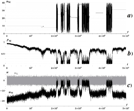
Figure 3: Dynamics of one realization from the polaron initial data. $N=40$, $T=15$, $\eta=0.456$, $\chi=0.2$, $\omega=0.1$ ($\chi/\omega=2$), $\gamma=3\omega$: a) position of the probability maximum in the chain (site number) $n_{M}(t)$, b) the value of $p_{M}(t)$, c) displacement of the $n_{M}$-th site $u_{M}$ (black) and the largest displacement $u_{K}$ in the “chain with window” (gray).

For $T\approx T_{crit}$ (e.g., in Fig. 2 for $N=40$, $T=15\approx T_{crit}$, $NT=600<NT_{crit}=650$), the dynamics of a realization in the thermodynamic equilibrium state is as follows: a polaron is formed at some site, exists for some time and then decays; for some time the charge can be considered to be delocalized over the whole of the chain, then a polaron “gathers” at another site, etc. Fig. 3 shows the results of modeling of one realization for the chain of $N=40$ sites at $T=15$. The initial stage of decaying of an “ideal” polaron is very large; for $t>2\cdot 10^{6}$ the system oscillates near TDE in the switching mode: for some time interval a charge is delocalized over the chain (e.g., from $t\approx 2.08\cdot 10^{6}$). In this case the location of probability maximum $n_{M}$ “jumps” over the whole of the chain (Fig. 3 a), the value of the maximum is $p_{M}\approx 0.2$ (Fig. 3 b). On this interval the displacement of the site with the maximum probability $u_{M}$ is close to $u_{K}$ (Fig. 3 c), i.e. this is not a polaron state. Then ($t\approx 2.15\cdot 10^{6}$) a charge is localized at one site ($n_{M}=25$, Fig. 3 a) with a high probability $p_{M}\approx 0.6$ (Fig. 3 b), besides $|u_{M}|>|u_{K}|$ (Fig. 3 c), i.e. a polaron “gathers” and exists for some time, then ($t\approx 2.3\cdot 10^{6}$) a charge again becomes delocalized, etc. Note that for small $T$ in the TDE (Fig. 2), $\langle R(T=5)\rangle\approx 1.24$ and $n_{M}(t)=const$ for each realization from polaron initial data; $\langle R(T=10)\rangle\approx 1.55$, and here we observed in 3 realizations of 50 very short periods of delocalization.

The dynamics in Fig. 3 is calculated for relatively slow values $\chi=0.2$, $\omega=0.1$, for which initial polaron disruption occurs during the time $t>10^{6}$. Fig. 4 shows a curve of the position $n_{M}(t)$ ($N=40$, $T=15$) for “adopted” values $\chi=1.$, $\omega=0.5$, which were used in most of the computer simulations. The initial polaron state disrupts during $t\sim 3\cdot 10^{4}$. Comparison of Figs. 3 a and 4 shows a qualitative similarity of the dynamics in the TDE – the periods of time when a charge is delocalized over the whole of the chain are changed by “polaron” intervals when a charge is localized at one site. Notice that sometimes the picture demonstrates “nearly polaron” transitions to the neighboring site, however the detailed consideration shows that the transition coincides with a delocalized state. Fig. 5 illustrates a fragment of the dynamics from Fig. 4 on the time interval $[122000,130000]$, where the jumps of the probability maximum to the neighboring site take place (for example, at $t\approx 125000$). During the transition the probability maximum $p_{M}$ decreases and the displacement of the site with the maximum is very close to displacements of other sites of the chain $u_{M}\approx u_{K}$, i.e. the charge can be considered to be delocalized. Regime in which a charge in the polaron state passes on from one site to another without delocalization intervals was not observed.

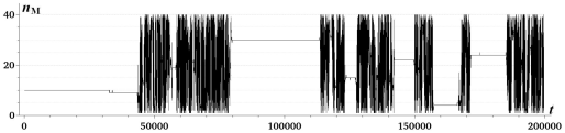
Figure 4: Position of a site with the probability maximum $n_{M}(t)$. One realization from the polaron initial data, $N=40$, $T=15$, $\eta=0.456$, $\chi=1.$, $\omega=0.5$, $\gamma=3\omega$.

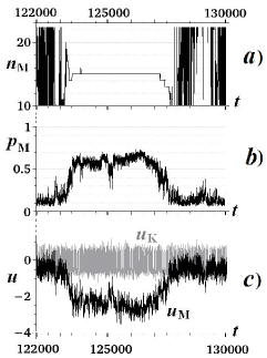
Figure 5: A fragment of the dynamics from Fig. 4 for the time $[122000,130000]$: a) the position $n_{M}$, b) the value of $p_{M}$, c) curves of $u_{M}$ (black) and $u_{K}$ (gray). The plots are matched with respect to time.

The friction coefficient $\gamma$ plays important role in modeling. To simulate the dynamics, we used rather large values of $\gamma>\omega$, which accelerate the achievement of the TDE state. For $\omega=0.5$ we tested small $\gamma$ values, the picture looks similar in quality, although the initial polaron disrupts more slowly. Fig. 6 shows a realization for $\gamma=0.02\omega=0.01$; the time interval of polaron disrupting $t\approx 5\cdot 10^{5}$, as for $\gamma=1.5$ (Fig. 4) initial polaron disrupts at $t\approx 4\cdot 10^{4}$.

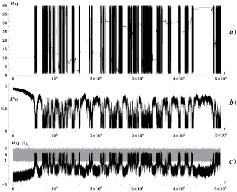
Figure 6: Dynamics of one realization from the polaron initial data. $N=40$, $T=15$, $\eta=0.456$, $\chi=1.$, $\omega=0.5$, $\gamma=0.01$. a) plot of $n_{M}(t)$, b) plot of $p_{M}(t)$, c) curves $u_{M}$ (black) and $u_{K}$ (gray).

Note that the similar picture of initial polaron destroying (Fig. 3 b for $t<2.1\cdot 10^{6}$ and Fig. 6 b for $t<5.5\cdot 10^{5}$) was calculated [48, 49] for the discrete nonlinear Schrödinger equation, which can be obtained as the limit of Holstein semiclassical model when charge transfer between sites is very slow compared to the site oscillations: $\eta\ll\omega$. We consider parameters $\eta\geq\omega$, and the time interval for initial polaron destroying at these parameters is much longer than in the works [48, 49].

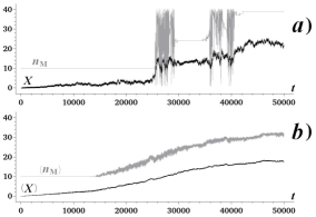
Figure 7: SRP in the electric field with intensity $V=0.01$. $N=40$, $T=15$, $\eta=0.456$, $\chi=1.$, $\omega=0.5$, $\gamma=3\omega$. a) The charge mass center $X(t)$ (black) and $n_{M}(t)$ (gray) for one realization, b) $\langle X(t)\rangle$ (black) and $\langle n_{M}(t)\rangle$ (gray) averaged over 50 realizations.

The results of simulation in the chain under the action of the field with intensity $V\neq 0$ show that in realizations the center of the polaron state is immobile (localized at one and the same site) until the polaron decays, in this time interval $p_{M}(t)$ decreases, displacement $u_{M}$ at this site decreases in modulus, but $n_{M}$ does not change (Fig. 7 a for $t<25000$). Then the charge passes on to the delocalized state and in this state migrates on an average in the field direction. Then the probability maximum is localized in the region of the sites with the lowest electron energy $\sim NV$. When averaging over realizations, since disruption of the initial polaron occurs at different points in time, more smooth curves are observed. Fig. 7 shows the curves of the charge mass center $X(t)$ (Eq. (12)) and $n_{M}(t)$ calculated for the intensity $V=0.01$ for one realization (Fig. 7 a), and $\langle X(t)\rangle$ and $\langle n_{M}(t)\rangle$ averaged over 50 trajectories (Fig. 7 b). The initial time interval $\langle X(t)\rangle$ (Fig. 7 b) $0<t<14000$ corresponds to the stage of polaron decay. The fragment $\langle X(t)\rangle$ for $16000<t<36000$ fits well the straight line and formally it can be used to estimate the average velocity of the charge $v$ (Eq. (13)). However this is not the polaron mechanism of the transfer, as is seen from Fig. 7 a.

Hence, the results of modeling demonstrate that for the SRP parameters in homogeneous chains a polaron does not move successively from one site to another. Here we deal with a switching mode between immobile polaron state and the delocalized one, and the transfer takes place in the delocalized state.

5 Results. Large Radius Polaron

Since for $T=0$ the highest probability (in the center of the polaron) is rather small ($p_{M}\approx 0.22$, Fig. 1) and, accordingly, the polaron displacements of the sites are small (Eq. (7)), the criterion of “polaron displacements” (which means that the greatest in modulus displacement will be of the site with the polaron center) is not always fulfilled here. Fig. 8 shows the time dependencies of the $n_{M}$ (Fig. 8 a) and $u_{M}$ (Fig. 8 b). It is seen that the polaron moves successively, however the displacements $u_{M}$ sometimes can be closer to zero than $u_{K}$ (Fig. 8 b).

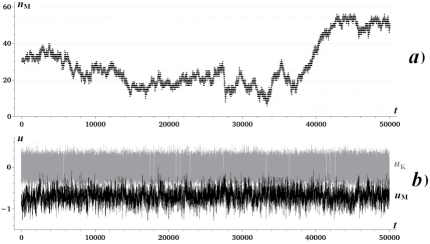
Figure 8: Large radius polaron (polyT fragment), $\eta=2.4$, $\chi=1.$, $\omega=0.5$, $\gamma=3\omega$. $N=60$, $T=3$ ($NT<NT_{crit}\approx 380$), one realization, at $t=0$ polaron with the center on the site $n_{0}=30$. a) Curve of $n_{M}(t)$, b) plots $u_{M}$ (black) and $u_{K}$ (gray).

As distinct from SRP, here the region of localized charge displaces successively from one site to another, i.e. LRP can moves along the chain. Therefore in this case we study time dependencies averaged over realizations.

In homogeneous chains disruption of polaron states depends on the heat energy of a chain $NT$ [27, 28]. At the same temperature $T$ in short chains ($NT<NT_{crit}$) a polaron exists while in long ones ($NT>NT_{crit}$) it decays. For the chains of different lengths, polaron decays with different rates. However, if at $t=0$ there is polaron in a chain, then for some time it exists. We investigate how polaron moves in chains of different lengths $N$ under the action of a field with constant intensity $V$.

The method of estimating the charge mobility $\mu$ for different $V$ (Eqs. (12),(13)) fails, since in the chains of different lengths the initial polaron decays differently. Fig. 9 shows the mean displacement of the charge center of mass $\langle X(t)\rangle$ (a), positions of the maximum $\langle n_{M}(t)\rangle$ (b), and the maximum probability $\langle p_{M}(t)\rangle$ (c) for the chains of different lengths in the field of intensity $|V|=0.001$ for $T=1$ (the sign of $V$ determines the direction of movement). For polyT parameters, the critical value is $NT_{crit}\approx 380$, i.e. for $T=1$ in the chains consisting of 200 sites a polaron exists, $N=400$ is near-border length of a chain and for the chain of 700 sites, a polaron decays.

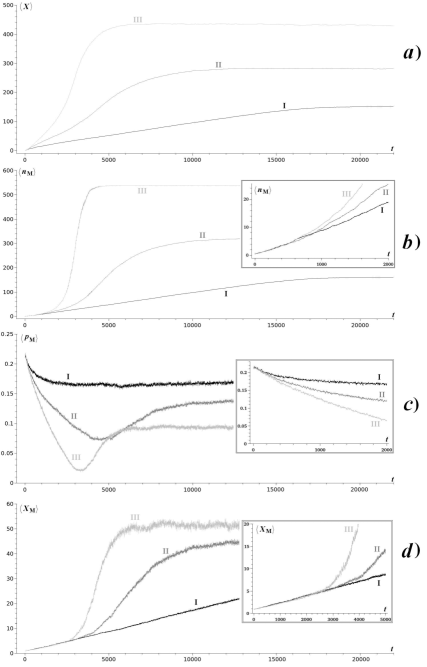
Figure 9: LRP, $\eta=2.4$, $\chi=1.$, $\omega=0.5$, $\gamma=\omega$, $T=1$, $V=-0.001$; chains of 200 sites (I, black), 400 sites (II, gray) and 700 sites (III, light gray). Each curve is mean over 100 realizations. The inserts demonstrate the zoomed initial stage. Initial polarons have center $n_{0}$ at the 20-th site for $N=200$, at the 70-th site for $N=400$, and at the 150-th site for $N=700$.

Fig. 9 (a–c) shows that $\langle X(t)\rangle$, $\langle n_{M}(t)\rangle$ and $\langle p_{M}(t)\rangle$ rather quickly diverge (at $t<500$). Curves III (for $N=700$) show that initial polaron moves gradually disrupting, and after $t\approx 2000$ velocity of $\langle n_{M}(t)\rangle$ increases greatly, and slope of $\langle X(t)\rangle$ changes. On this time polaron disrupts, and then waves of $b_{n}$ move along the field direction. At $t\approx 4000$ $\langle p_{M}(t)\rangle$ reaches the end of the chain (after that $\langle n_{M}(t)\rangle$ does not change), and then the probability maximum is localized in the region of the sites with the lowest electron energy $\sim NV$ and gradually $p_{M}(t)$ increases. And after $t\approx 6000$ this system attains new thermodynamic equilibrium state ($\langle X(t>6000)\rangle\approx const$, as well as $\langle n_{M}(t)\rangle$ and $\langle p_{M}(t)\rangle$). For 400-site chain (curves II), the picture is qualitatively similar, but more extended in time. And for $N=200$ (curves I) at $t\approx 2000$ polaron is formed corresponding to this conditions ($T$ and $V$), and polaron moves along the chain; at $t\approx 18000$ it reaches the end of the chain (after that $\langle X(t)\rangle\approx const$, $\langle n_{M}(t)\rangle\approx const$, Fig. 9 a),b).

The slope of $\langle X(t)\rangle$ in the initial interval (as long as polaron exists) is different for different $N$; e.g., in Fig. 9 a) these intervals are: $t<1400$ for $N=700$, $t<2700$ for $N=400$, and $t<18000$ for $N=200$. As shown in Fig. 10, the difference decreases with decreasing temperature and for $T=0$ $dX(t)/dt$ is the same for all chains with length $N\gg R(T=0)$.

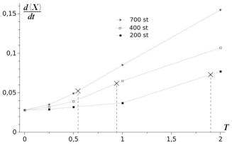
Figure 10: The slope of $\langle X(t)\rangle$ in the initial interval (as long as polaron exists) at $T=0.25,0.5,1,2$ for chains of $N=200$ sites (black squares), $N=400$ (open squares), $N=700$ (stars). LRP, $\eta=2.4$, $\chi=1.$, $\omega=\gamma=0.5$, $V=0.005$. The crosses indicate the conditional boundary $NT=380$ between the polaron and delocalized states in the TDE at a given chain length.

Instead of $\langle X(t)\rangle$ we calculated truncated variant $\langle X_{M}(t)\rangle$ (Eq. (14)) where only the motions of the polaron top are used, see Fig. 9 d. Calculations demonstrate that for chains of different lengths, the curves $\langle X_{M}(t)\rangle$ coincide on a far greater time interval, than $\langle X(t)\rangle$, $\langle n_{M}(t)\rangle$ and $\langle p_{M}(t)\rangle$: in Fig. 9 d the common segment $t>2500$, separation of the other plots becomes noticeable at a far lesser time. Notice that for a 200-site chain (black line (I) in Fig. 9), in which a polaron does not decay in TDE at $T=1$, $\langle X_{M}(t)\rangle$ behaves like a straight line until a polaron reaches the end of chain. For still longer chains, a polaron decays at some moment of time which is evident from a sharp change in $\langle X_{M}(t)\rangle$ (for a 400-site chain (II) $t\approx 4000$, and for a 700-site chain (III) $t\approx 2500$).

By analogy with the estimation of the charge mobility (12),(13) for intensity $V\neq 0$, based on $\langle X_{M}(t)\rangle=v_{M}t$ we estimate the “mean velocity of the polaron” $v_{M}$ for different $V$ and get a “polaron mobility” $\mu_{M}$ by substituting $v_{M}=\mu_{M}V$.

Table 1 lists the results of calculations of $v_{M}$ based on the slope of the linear fragment $\langle X_{M}(t)\rangle$ averaging over 100 realizations, common for the chains of different lengths. The simulations are performed for different $T$, the parameter values are $\eta=2.4$, $\chi=1.$, $\omega=0.5$, $\gamma=0.3$. It is evident that the change in $V$ is proportional to the change in $v_{M}$. Though the values of $T$ grow twice, the calculated values of $\mu_{M}$ are very close and therefore one cannot single out the dependence $\mu_{M}(T)$. The dependence of $\mu_{M}(T)$ for small $T$ can be more exactly due to quadratic increase in the number of realizations which is computationally expensive. The calculations carried out suggest that the polaron mobility for $T\to 0$ is very small, substitution of the DNA parameter values leads to $\tilde{\mu}=(ea^{2}/\hbar)\mu_{M}\approx 0.005$ cm${}^{2}/$(V$\cdot$sec). Notice that for $T=0$ (Eq. (12),(13)) the charge mobility is $\mu_{0}\approx 9.2$, and the polaron mobility $\mu_{M0}\approx 2.0=\mu_{0}p_{M}$ (since for $T=0$ the polaron velocity measured from $n_{M}(t)$ coincides with $\Delta X/\Delta t$) is close to the values of Table 1.

Table 1: Polaron velocity $v_{M}$ and mobility $\mu_{M}$

$T$	$v_{M}$, $N=200$	$v_{M}$, $N=400$	$v_{M}$, $N=700$	$\mu_{M}=v_{M}/V$
	$V=0.0005$	$V=0.001$	$V=0.005$
0.25	0.0012	0.0023	0.011	2.2-2.4
0.5	0.0013	0.0023	0.012	2.3-2.6
1.	0.0012	0.0024	0.012	2.4

For LRP the value of $\gamma$ is significant. At $T=0$ for fixed $V$ velocity of polaron depends on $\gamma$ [14], the smaller $\gamma$, the greater velocity. Fig. 11 shows $\langle X_{M}(t)\rangle$ for different $\gamma$ at $T=1$. For $\gamma=3$ slope of $\langle X_{M}(t)\rangle$ is small, and for chains $N=400$ and $N=700$ the initial polaron has time to disrupt. For $\gamma=0.03$ slope of $\langle X_{M}(t)\rangle$ is large and for all chains polaron manages to reach the end of the chains.

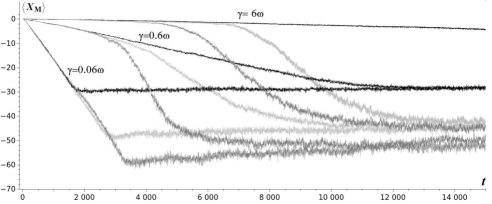
Figure 11: $\langle X_{M}(t)\rangle$ for $N=200$ (black curves), $N=400$ (light gray) and $N=700$ (gray). $T=1$, $\eta=2.4$, $\chi=1.$, $\omega=0.5$, $V=0.001$ (initial polarons are localized near right end of the chain, the center of the polaron is at the same distance from the right end as in Fig. 9); different $\gamma$ values.

Also the ratio $\eta/\omega$ is important for demonstration of chain length effects. Fig. 12 shows $\langle X(t)\rangle$ and $\langle X_{M}(t)\rangle$ of dynamics of the initial polaron (averaged over 24 realizations) for $\eta=2.4$ and different values of $\chi,\omega$ with the same ratio $\chi/\omega=2$ (subscripts in Fig. 12 denote chain length). Although in the TDE state the mean values should be the same, but the time to attain it may be very long. For curves 3 in Fig. 12 with ($\chi=0.02,\omega=0.01$) on this time of integration there is no noticeable difference in the curves for $N=200$ ($3_{200}$) and $N=400$ ($3_{400}$) for $\langle X(t)\rangle$ and $\langle X_{M}(t)\rangle$. Note that for “realistic” DNA parameter values in Holstein model [40, 41], $\eta/\omega$ is of the order of hundreds, and results are similar to curves 3.

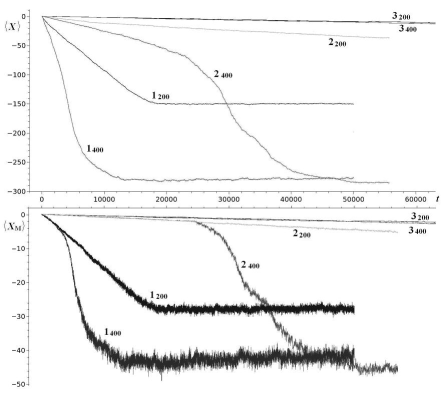
Figure 12: Curves $\langle X(t)\rangle$ (top) and $\langle X_{M}(t)\rangle$ (bottom) for chains of 200 and 400 sites (subscript denotes chain length). $T=1$, $\eta=2.4$, $V=0.001$, $\gamma=\omega$, initial polarons are localized as in Fig. 9. Parameters for curves (1): $\chi=1.$, $\omega=0.5$; for (2): $\chi=0.2$, $\omega=0.1$; for (3): $\chi=0.02$, $\omega=0.01$.

6 Discussion and conclusions

Using a computational experiment we studied the dynamics of a polaron in a chain with Langevin thermostat under the action of a constant electric field. We considered the cases of a small radius polaron and a large radius polaron.

It is shown that for the parameters corresponding to small radius polaron, the polaron is immobile. Calculations of dynamics demonstrate that polaron exists for some time and then decays; for some time the charge is delocalized over the whole chain, then a polaron “gathers” at another random site. Charge transfer takes place in the delocalized state, i.e., for the SRP parameters, a charge does not move along the chain like a polaron. In this work we consider possibility of charge transfer by polaron mechanism; a number of interesting questions, e.g. mean ratio of time intervals “polaron/delocalized state” in the TDE, or how time of initial polaron destroying depends on $N$ and $T$ will be studied later.

Theoretical models of SRP motion imply that a polaron under the action of temperature fluctuations hops from one site to the neighboring one or to one of the neighboring sites within a small region [26, 50, 51, 52]. We calculated the dynamics in the chains consisting of 40 to 200 sites. The results demonstrate that a charge in the delocalized state is “spread” over the whole chain rather than over some of its regions with the center of the former polaron, and the position of the new polaron which gathered after delocalization interval is not related to the position of the previous polaron. It looks like intermittency in dynamical systems [53].

This behavior depends on the polaron radius $R$; for polyC chains ($R\approx 1.2$, matrix element $\eta=0.623$, $\nu=0.041$ eV [40, 41]) on some time intervals there is a consistent polaron movement, but such intervals are separated by intervals of delocalization along the whole chain; for polyA ($R\approx 1.07$) and Holstein SRP ($R\approx 1.02$, parameters from footnote 17 of [26]) such consistent polaron motion was not observed.

Perhaps, at very small $T$, this regime passes into the hopping mechanism considered by Holstein [26] or variable range hopping [50]. Directly during simulations, we did not observe such regimes (and we do not know the papers in which the authors observed such regimes in direct simulations), possibly because theoretically in this case the charge is localized at one site for a very long time.

Large radius polaron can move over the chain. In the semiclassical Holstein model the region of existence of polaron in thermodynamic equilibrium state depends not only on temperature but also on the chain length. Therefore in modeling from initial polaron data the slope of $\langle X(t)\rangle=\langle\sum_{n}p_{n}(n-n_{0})\rangle$ differs for the chains of different lengths at the same temperature. We showed numerically that for the chains of different lengths, the “polaron center mass” $\langle X_{M}(t)\rangle=\langle p_{M}(n_{M}-n_{0})\rangle$ behaves similarly until the polaron decays (for the same $T$ and intensity $V$ of electric field). A similar slope $\langle X_{M}(t)\rangle$ enables one to find the mean polaron velocity and, by analogy with the charge mobility, estimate the polaron mobility $\mu_{M}$. The calculated values of $\mu_{M}$ for small $T$ are close to the value at $T=0$, which does not contradict the assumption $\mu_{M}(T\to 0)=\mu_{M}(0)$. The calculations performed demonstrate that at zero temperature the polaron mobility is small but nonzero. These results agree with earlier obtained data on the Holstein polaron motion along an unperturbed chain (for $T=0$) [14, 16].

We considered a simple model, classical chain without dispersion (in [54] dispersion is used to model stacking interaction of the DNA strand). More detailed Peyrard–Bishop model with nonlinear interaction between neighboring base pairs [55, 56] for the case of small site displacements can be reduced to the form similar to that of the dispersion term in equations for crystals. The values of the charge mobility in DNA obtained in some works on the basis of different models are very small [57, 58, 59]. For this reason different mechanisms of charge transfer with the use of nonlinear excitations are studied [54, 60, 61]. It has been found that a metastable quasi-particle may be transported at a distance up to 200 base pair [62, 63] without an external electric field. Such mechanism may be considered as an alternative one to the polaron mechanism.

According to the results of modeling, for the LRP parameter values the charge transfers faster in the delocalized state. Thus, in Fig. 9 it is shown that in 700-site chain the charge maximum $n_{M}$ reaches the end at the time $t\approx 5000$. The same time interval is taken to “gather” the probability at the end of a chain, the greatest value is $\langle p_{M}(t=10000)\rangle\approx 0.09$. While for the 200-site chain polaron passes it during $t\approx 20000$, but the probability maximum is always $\langle p_{M}\rangle>0.15$. Which regime is better (and can these modes be realized in experiments) – it is the problem for further investigations.

The ratio $\eta/\omega$ is important for observing chain length effects, such as difference in $\langle X(t)\rangle$, $\langle p_{M}(t)\rangle$, $\langle n_{M}(t)\rangle$ for different $N$. The larger this ratio, the smaller the difference in the slopes of $\langle X(t)\rangle$ at the same $V$.

We consider the chains with free ends. For $V=0$ we made several numerical tests (for SRP $N=40$, $T=10$, $T=15$, and for LRP $N=200$ and $N=700$, $T=1$) in circle chain (i.e., periodic boundary conditions). The test results (averaged values) are similar. For $V\neq 0$ this question needs further research.

We carried out numerical simulations for some sets of parameter values, with $\chi\approx\omega$, $\eta\geq\omega$. Based on this extensive work, we can expect that qualitatively similar pattern of the polaron dynamics exists in a wide range of parameters. Probably, direct simulations in other mixed quantum-classical models with Langevin term [22, 29, 64, 65] might demonstrate some similar features of polaron dynamics, different dynamics at the same temperature in the chains with different length, such as dependence of $\langle p_{M}(t)\rangle$ or $\langle X(t)\rangle$ on the chain length.

References

- [1] A. Scott, Nonlinear science. Emergence and dynamics of coherent structures (2nd ed.), Oxford University Press (2003) 496 p.doi:ISBN 9783540201311.
- [2] G. Schuster (ed.), Long-range charge transfer in DNA II, Topics in Current Chemistry 237 (2004) 245 p. doi:ISBN 978-3-540-20131-1.
- [3] A. Alexandrov (ed.), Polarons in advanced materials, Springer Series in Materials Science 103 (2007) 672 p. doi:10.1007/978-1-4020-6348-0.
- [4] S. Flach, A. Gorbach, Discrete breathers – advances in theory and applications, Physics Reports 467 (1–3) (2008) 1–116. doi:10.1016/j.physrep.2008.05.002.
- [5] M. Johansson, G. Kopidakis, S. Lepri, S. Aubry, Transmission thresholds in time-periodically driven nonlinear disordered systems, Europhysics Letters 86 (1) (2009) 10009–7. doi:10.1209/0295-5075/86/10009.
- [6] M. Samuelsen, A. Khare, A. Saxena, K. Rasmussen, Statistical mechanics of a discrete schrodinger equation with saturable nonlinearity, Physical Review E 87 (4) (2013) 044901. doi:10.1103/PhysRevE.87.044901.
- [7] L. Cisneros-Ake, L. Cruzeiro, M. Velarde, Mobile localized solutions for an electron in lattices with dispersive and non-dispersive phonons, Physica D – Nonlinear Phenomena 306 (2015) 82–93. doi:10.1016/j.physd.2015.05.008.
- [8] S. Iubini, S. Lepri, R. Livi, G. Oppo, A. Politi, A chain, a bath, a sink, and a wall, Entropy 19 (9) (2017) 445–15. doi:10.3390/e19090445.
- [9] E. Starikov, S. Tanaka, J. Lewis (eds.), Modern methods for theoretical physical chemistry of biopolymers, Elsevier Scientific, Amsterdam (2006) 461 p.doi:ISBN 9780444522207.
- [10] T. Chakraborty (ed.), Charge migration in DNA. Perspectives from physics, chemistry, and biology, Springer, Berlin (2007) 288 p.doi:10.1007/978-3-540-72494-0.
- [11] A. Offenhäusser, R. Rinaldi (eds.), Nanobioelectronics – for electronics, biology, and medicine, Springer, New York (2009) 337 p.doi:10.1007/978-0-387-09459-5.
- [12] V. Lakhno, DNA nanobioelectronics, International Journal of Quantum Chemistry 108 (11) (2008) 1970–1981. doi:10.1002/qua.21717.
- [13] V. Lakhno, Davydov’s solitons in homogeneous nucleotide chain, International Journal of Quantum Chemistry 110 (1) (2010) 127–137. doi:10.1002/qua.22264.
- [14] V. Lakhno, A. Korshunova, Electron motion in a Holstein molecular chain in an electric field, The European Physical Journal B 79 (2) (2011) 147–151. doi:10.1140/epjb/e2010-10565-2.
- [15] Z. Huang, L. Chen, N. Zhou, Y. Zhao, Transient dynamics of a one-dimensional Holstein polaron under the influence of an external electric field, Annalen der Physik 529 (5) (2017) 1600367–12. doi:10.1002/andp.201600367.
- [16] A. Korshunova, V. Lakhno, Simulation of the stationary and nonstationary charge transfer conditions in a uniform Holstein chain placed in constant electric field, Technical Physics 63 (9) (2018) 1270–1276 —. doi:10.1134/S1063784218090086.
- [17] Z. Huang, M. Hoshina, H. Ishihara, Y. Zhao, Transient dynamics of super Bloch oscillations of a 1d Holstein polaron under the influence of an external AC electric field, Annalen der Physik 531 (1) (2019) 1800303–11. doi:10.1002/andp.201800303.
- [18] P. Lomdahl, W. Kerr, Do Davydov solitons exist at 300 K?, Physical Review Letters 55 (11) (1985) 1235–1238. doi:10.1103/PhysRevLett.55.1235.
- [19] D.Vitali, P.Allegrini, P.Grigolini, Nonlinear quantum mechanical effects: real or artefact of inaccurate approximations?, Chemical Physics 180 (2–3) (1994) 297–318. doi:10.1016/0301-0104(93)E0416-S.
- [20] M. Salkola, A. Bishop, V. Kenkre, S. Raghavan, Coupled quasiparticle-boson systems: The semiclassical approximation and discrete nonlinear Schrœdinger equation, Physical Review B 52 (6) (1995) R3824. doi:10.1103/PhysRevB.52.R3824.
- [21] A. Savin, A. Zolotaryuk, Dynamics of the amide-I excitation in a molecular chain with thermalized acoustic and optical modes, Physica D: Nonlinear Phenomena 68 (1) (1993) 59–64. doi:10.1016/0167-2789(93)90029-Z.
- [22] L. Cruzeiro-Hansson, S. Takeno, Davydov model: The quantum, mixed quantum-classical, and full classical systems, Physical Review E 56 (1) (1997) 894–906. doi:10.1103/PhysRevE.56.894.
- [23] W. Ebeling, M. Velarde, A. Chetverikov, Bound states of electrons with soliton-like excitations in thermal systems. Adiabatic approximations, Condensed Matter Physics 12 (4) (2009) 633–645. doi:10.5488/CMP.12.4.633.
- [24] V. Lakhno, N. Fialko, Hole mobility in a homogeneous nucleotide chain, Journal of Experimental and Theoretical Physics Letters 78 (5) (2003) 336–338. doi:10.1134/1.1625737.
- [25] V. Lakhno, N. Fialko, Bloch oscillations in a homogeneous nucleotide chain, Journal of Experimental and Theoretical Physics Letters 79 (10) (2004) 464–467. doi:10.1134/1.1780553.
- [26] T. Holstein, Studies of polaron motion: Part II. The “small” polaron, Annals of Physics 8 (3) (1959) 343–389. doi:10.1016/0003-4916(59)90003-X.
- [27] V. Lakhno, N. Fialko, On the dynamics of a polaron in a classical chain with finite temperature, Journal of Experimental and Theoretical Physics 120 (1) (2015) 125–131. doi:10.1134/S106377611501015X.
- [28] N. Fialko, E. Sobolev, V. Lakhno, On the calculation of thermodynamic quantities in the Holstein model for homogeneous polynucleotides, Journal of Experimental and Theoretical Physics 124 (4) (2017) 635–642. doi:10.1134/S1063776117040124.
- [29] G. Kalosakas, K. Rasmussen, A. Bishop, Charge trapping in DNA due to intrinsic vibrational hot spots, Journal of Chemical Physics 118 (8) (2003) 3731–3735. doi:10.1063/1.1539091.
- [30] Z. Qu, D. Kang, H. Jiang, S. Xie, Temperature effect on polaron dynamics in DNA molecule: The role of electron-base interaction, Physica B 405 (2010) S123 S125. doi:10.1016/j.physb.2009.12.020.
- [31] J. Dong, W. Si, C.-Q. Wu, Drift of charge carriers in crystalline organic semiconductors, Journal of Chemical Physics 144 (2016) 144905–8. doi:10.1063/1.4945778.
- [32] N. Voulgarakis, The effect of thermal fluctuations on Holstein polaron dynamics in electric field, Physica B 519 (2017) 15–20. doi:10.1016/j.physb.2017.04.030.
- [33] Y. Yao, Y. Qiu, C.-Q. Wu, Dissipative dynamics of charged polarons in organic molecules, Journal of Physics: Condensed Matter 23 (2011) 305401–6. doi:0953-8984/23/30/305401.
- [34] S. Bhattacharyya, S. Bakshi, S. Kadge, P. Majumdar, Langevin approach to lattice dynamics in a charge-ordered polaronic system, Physical Review B 99 (2019) 165150. doi:10.1103/PhysRevB.99.165150.
- [35] G. Kalosakas, K. Rasmussen, A. Bishop, Nonlinear excitations in DNA: polarons and bubbles, Synthetic Metals 141 (2004) 93–97. doi:10.1016/j.synthmet.2003.08.020.
- [36] S. Behnia, S. Fathizadeh, Modeling the electrical conduction in DNA nanowires: Charge transfer and lattice fluctuation theories, Physical Review E 91 (2015) 022719–10. doi:10.1103/PhysRevE.91.022719.
- [37] S. Fratini, D. Mayou, S. Ciuchi, The transient localization scenario for charge transport in crystalline organic materials, Advanced Functional Materials 26 (2016) 2292–2315. doi:10.1002/adfm.201502386.
- [38] T. Holstein, Studies of polaron motion: Part I. The molecular-crystal model, Annals of Physics 8 (3) (1959) 325–342. doi:10.1016/0003-4916(59)-90002-8.
- [39] E. Helfand, Brownian dynamics study of transitions in a polymer chain of bistable oscillators, The Journal of Chemical Physics 69 (3) (1978) 1010–1018. doi:10.1063/1.436694.
- [40] A. Voityuk, N. Rösch, M. Bixon, J. Jortner, Electronic coupling for charge transfer and transport in DNA, The Journal of Physical Chemistry B 104 (41) (2000) 9740–9745. doi:10.1021/jp001109w.
- [41] J. Jortner, M. Bixon, A. Voityuk, N. Rösch, Superexchange mediated charge hopping in DNA, The Journal of Physical Chemistry A 106 (33) (2002) 7599–7606. doi:10.1021/jp014232b.
- [42] F. Lewis, Y. Wu, Dynamics of superexchange photoinduced electron transfer in duplex DNA, Journal of Photochemistry and Photobiology C 2 (1) (2001) 1–16. doi:10.1016/S1389-5567(01)00008-9.
- [43] K.-H. Yoo, D. Ha, J.-O. Lee, J. Park, J. Kim, J. Kim, H.-Y. Lee, T. Kawai, H. Y. Choi, Electrical conduction through Poly(dA)-Poly(dT) and Poly(dG)-Poly(dC) DNA molecules, Physical Review Letters 87 (19) (2001) 198102–4. doi:10.1103/PhysRevLett.87.198102.
- [44] S. Patwardhan, S. Tonzani, F. Lewis, L. Siebbeles, G. Schatz, F. Grozema, Effect of structural dynamics and base pair sequence on the nature of excited states in DNA hairpins, Journal of Physical Chemistry B 116 (2012) 11447–11458. doi:10.1021/jp307146u.
- [45] A. Chetverikov, W. Ebeling, M. Velarde, On the temperature dependence of fast electron transport in crystal lattices, The European Physical Journal B 88 (2015) 202–7. doi:10.1140/epjb/e2015-60495-4.
- [46] H. Greenside, E. Helfand, Numerical integration of stochastic differential equations – II, Bell System Technical Journal 60 (8) (1981) 1927–1940. doi:10.1002/j.1538-7305.1981.tb00303.x.
- [47] N. Fialko, Mixed algorithm for modeling of charge transfer in DNA on long time intervals (in russ.), Computer Research and Modeling 2 (1) (2010) 63–72. doi:10.20537/2076-7633-2010-2-1-63-72.
- [48] P. Christiansen, Y. Gaididei, M. Johansson, K. Rasmussen, Breatherlike excitations in discrete lattices with noise and nonlinear damping, Physical Review B 55 (9) (1997) 5759–5766. doi:10.1103/PhysRevB.55.5759.
- [49] K. Rasmussen, P. Christiansen, M. Johansson, Y. Gaididei, S. Mingaleev, Localized excitations in discrete nonlinear schredinger systems: Effects of nonlocal dispersive interactions and noise, Physica D: Nonlinear Phenomena 113 (2-4) (1998) 134–151. doi:10.1016/S0167-2789(97)00261-3.
- [50] N. Mott, E. Davis, Electronic processes in non-crystalline materials, Clarendon Press, Oxford (2nd ed.)doi:ISBN 9780199645336.
- [51] J. Devreese, A. Alexandrov, Fröhlich polaron and bipolaron: recent developments, Reports on Progress in Physics 72 (6) (2009) 066501–53. doi:10.1088/0034-4885/72/6/066501.
- [52] M. Zoli, Polaron mass and electron-phonon correlations in the Holstein model, Advances in Condensed Matter Physics, 2010 (2010) 815917–15. doi:10.1155/2010/815917.
- [53] H. Schuster, Deterministic chaos: An introduction, Physik-Verlag (1984) 220 p.doi:ISBN: 978-0895736116.
- [54] S. Komineas, G. Kalosakas, A. Bishop, Effects of intrinsic base-pair fluctuations on charge transport in DNA, Physical Review E 65 (6) (2002) 061905. doi:10.1103/PhysRevE.65.061905.
- [55] M. Peyrard, A. Bishop, Statistical mechanics of a nonlinear model for DNA denaturation, Physical Review Letters 62 (23) (1989) 2755. doi:10.1103/PhysRevLett.62.2755.
- [56] T. Dauxois, M. Peyrard, A. Bishop, Entropy-driven DNA denaturation, Physical Review E 47 (1) (1993) R44. doi:10.1103/PhysRevE.47.R44.
- [57] D. Basko, E. Conwell, Effect of solvation on hole motion in DNA, Physical Review Letters 88 (9) (2002) 098102–1. doi:10.1103/PhysRevLett.88.098102.
- [58] A. Voityuk, Charge transfer in DNA: Hole charge is confined to a single base pair due to solvation effects, The Journal of Chemical Physics 122 (20) (2005) 204904. doi:10.1063/1.1924551.
- [59] E. Conwell, D. Basko, Effect of water drag on diffusion of drifting polarons in DNA, The Journal of Physical Chemistry B 110 (46) (2006) 23603–23606. doi:10.1021/jp064373j.
- [60] J. Cuevas, P. Kevrekidis, D. Frantzeskakis, A. Bishop, Existence of bound states of a polaron with a breather in soft potentials, Physical Review B 74 (6) (2006) 064304–12. doi:10.1103/PhysRevB.74.064304.
- [61] A. Chetverikov, W. Ebeling, V. Lakhno, A. Shigaev, M. Velarde, On the possibility that local mechanical forcing permits directionally-controlled long-range electron transfer along DNA-like molecular wires with no need of an external electric field, The European Physical Journal B 89 (4) (2016) 101. doi:10.1140/epjb/e2016-60949-1.
- [62] A. Chetverikov, K. Sergeev, V. Lakhno, Trapping and transport of charges in DNA by mobile discrete breathers, Mathematical Biology and Bioinformatics 13 (1) (2018) 1–12. doi:10.17537/2018.13.1.
- [63] A. Chetverikov, W. Ebeling, V. Lakhno, M. Velarde, Discrete-breather-assisted charge transport along DNA-like molecular wires, Physical Review E 100 (5) (2019) 052203–9. doi:10.1103/PhysRevE.100.052203.
- [64] G. Kalosakas, K. Rasmussen, A. Bishop, Nonlinear excitations in DNA: polarons and bubbles, Synthetic Metals 141 (1-2) (2004) 93 –97. doi:10.1016/j.synthmet.2003.08.020.
- [65] L. Ribeiro, W. Cunha, P. Neto, R. Gargano, G. Silva, Effects of temperature and electric field induced phase transitions on the dynamics of polarons and bipolarons, New Journal of Chemistry 37 (9) (2013) 2829–2836. doi:10.1039/c3nj00602f.