Experimental Evaluation of 3D-LIDAR Camera Extrinsic Calibration

Abstract

In this paper we perform an experimental comparison of three different target based 3D-LIDAR camera calibration algorithms. We briefly elucidate the mathematical background behind each method and provide insights into practical aspects like ease of data collection for all of them. We extensively evaluate these algorithms on a sensor suite which consists multiple cameras and LIDARs by assessing their robustness to random initialization and by using metrics like Mean Line Re-projection Error (MLRE) and Factory Stereo Calibration Error. We also show the effect of noisy sensor on the calibration result from all the algorithms and conclude with a note on which calibration algorithm should be used under what circumstances.

I Introduction

3D-LIDARs and cameras are ubiquitous to robots. Cameras provide color, texture and appearance information which LIDARs lack and LIDARs provide depth information which cameras lack. Virtually all modern autonomy stacks use multiple distinct types of sensors to represent and interact in the external environment, and many high-level autonomy behaviors (multi-modal object detection, state-estimation, mobile manipulation, etc.) depend on accurate calibrations between sensors, such that data from all sensors can be expressed in a common spatial frame of reference. Yet, there is still no unified approach for calibrating the various sensors present on most autonomous systems. This has motivated research for estimation of extrinsic calibration between various sensors, such as 3D-LIDARs and cameras. Although this area has seen contributions from various robotics labs and research groups, a comprehensive work which analyzes commonly used methods and provides experimental evaluation is lacking. In this work, we experimentally evaluate commonly used methods for estimating 3D-LIDAR-to-camera extrinsic calibration, offering insights into the strengths and weaknesses of various formulations and providing interesting avenues for further work.

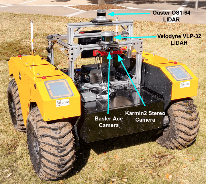
Figure 1: Experimental Platform: Clearpath Robotics Warthog UGV with $a).$ Ouster OS1 LIDAR, $b).$ Velodyne VLP-32 LIDAR, $c).$ Karmin2 Stereo Camera & $d).$ Basler Ace Camera

I-A Literature Survey

Existing 3D-LIDAR camera extrinsic calibration algorithms can be broadly classified into target based [1], [2], [3], [4], [5], and targetless approaches [6], [7], [8], [9]. A target based approach requires a known object in the sensors’ common Field of View (FoV) to establish geometric constraints between features detected across the calibrated sensors. While targetless approaches have the obvious advantage of not requiring any special environmental augmentation, reliable accurate data association across modalities is still an open research problem. Although, for many purposes, approximate data association is sufficient (for example, using a camera-based object detection to project a semantic label to a cluster of lidar points), calibration is a problem which uniquely demands metric accuracy above all else. Therefore, approximate data associations with no prior initialization will lead to poor calibration results, which is why even targetless calibration techniques still depend on accurate target based calibration as a precursor. While the ultimate goal of our research is to enable accurate online targetless calibration in arbitrary environments, here we focus on the offline target based calibration to identify the best in class approaches to data association and multi-sensor optimization.

The solution to target based 3D-LIDAR camera extrinsic calibration problem is inspired from target based 2D-LIDAR camera extrinsic calibration [10], [11], [12], [13], etc. The geometric constraint used in [11] is easy to use in 3D-LIDAR camera calibration scenario and has been exploited in the work presented in [1] & [2] and extended to 3D-LIDAR omnidirectional camera calibration in [3]. [4] present a 3D-LIDAR camera calibration technique in which the rotation matrix is estimated first and then a point to plane constraint (similar to ones in [1], [2], [3]) is used to determine the transformation parameters. [5] adds more geometric constraints by introducing line correspondences in addition to the previously used plane correspondences. [1], [2], [3], [4] and [5] use a planar target with a checkerboard pattern. [14] and [15] present calibration methods that use a rigid plane with one and four circular perforations respectively. The methods involve detection of circle in both the image and the 3D-LIDAR data and using the geometric constraints to determine the SE(3) transformation between the 3D-LIDAR and the camera. All of the aforementioned methods which use a single planar target require several observations from geometrically distinct view points. [16] presents a single view calibration technique, but uses several checkerboard planes. In addition to the point to plane geometric constraint that form the basis of methods described in [1], [2] and [3], the point to back-projected plane constraint has been exploited in works described in [12] and [13], but only for calibrating 2D-LIDAR camera systems. [17] exploits the point to back-projected plane constraint for cross calibrating 3D LIDAR camera pair. The methods described so far are pair-wise 3D-LIDAR camera calibration techniques. For robots with multiple cameras and LIDARs, joint calibration techniques like [18] and [19] have been found to be useful. Most target based 2D/3D-LIDAR camera extrinsic calibration methods, which use one or more planar surfaces, use checkerboards or ArUco [20] or AprilTags [21] for easy detection of planar target in the camera. In cases where such markers are not used, perforated [14] & [15] or spherical targets [22] are utilized.

I-B Contributions

In this work, we experimentally evaluate three different 3D-LIDAR camera extrinsic calibration algorithms, specifically those presented in [2], [17] and [19]. Unlike [2] and [17] which are pair wise 3D-LIDAR camera calibration algorithms, [19] is a multi-sensor graph based optimization algorithm that jointly calibrates an arbitrary set of such sensors. We have evaluated these algorithm on the sensor suite shown in Figure 2, and have demonstrated the varying robustness of each approach to noisy sensor data. All three methods compared here use a planar target (with known physical characteristics) as the calibration object.

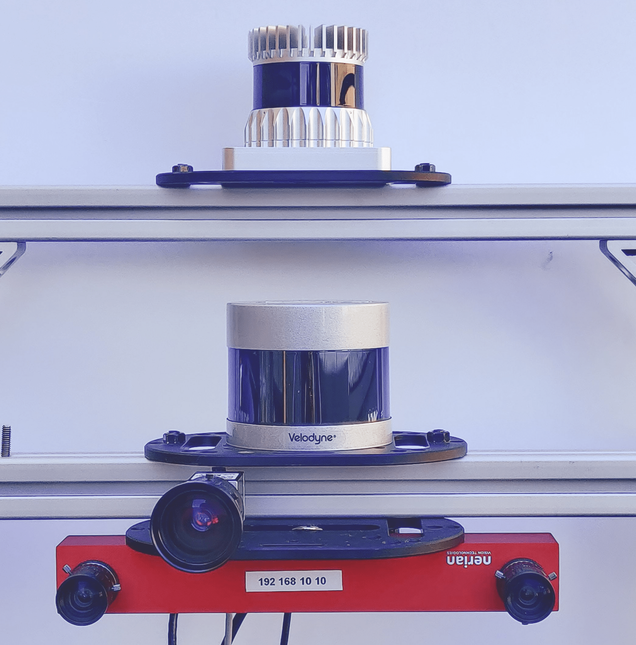
Figure 2: Sensors (From Top to Bottom): Ouster OS1 64 Channel LIDAR, Velodyne VLP-32 LIDAR, Basler Ace Camera and Karmin2 Stereo Camera.

II 3D-LIDAR Camera Calibration

II-A The Problem

For the pinhole camera model, the relationship between a homogeneous 3D point, ${P}^{L}_{i}$, and its homogeneous image projection $p^{C}_{i}$, is given by

$$p^{C}_{i}=K[^{C}R_{L},^{C}t_{L}]P^{L}_{i}.$$ (1)

The extrinsic parameters that transform the laser coordinate system to that of the camera are captured by $[{}^{C}R_{L},{}^{C}t_{L}]$, where ${}^{C}R_{L}$ is the orthonormal rotation matrix and $t^{C}_{L}:=[x,y,z]^{\top}$ is the translation vector between the two coordinate frames. The camera intrinsics are captured by the matrix $K$ and is assumed to be known or estimated using established monocular calibration methods (e.g., [23]). The methods evaluated here require a planar target that is visible in both camera and lidar frame in order to establish the geometric constraints that allow us to estimate the rigid body transformation $[{}^{C}R_{L},{}^{C}t_{L}]$ between the two sensors (Figure 3).

II-B Notations

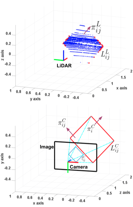
Figure 3: Notations: In LIDAR, the $i^{th}$ pose of the planar target yields planar points $\{P^{L}_{im}\}$ (blue, where $m=\{1,2,...,p_{i}\}$ & $p_{i}$ is the number of points detected on the planar surface) and boundary points $\{Q^{L}_{ijn}\}$ (red, where $j=\{1,2,3,4\}$ & $n=\{1,...,q_{ij}\}$, $q_{ij}$ is the number of points on $j^{th}$ line). In Camera, the $i^{th}$ pose of the planar target yields lines ${l^{C}_{ij}}$ (where $j=\{1,2,3,4\}$) and planes $\pi^{C}_{i}$ & $\pi^{C}_{ij}$ (where $j=\{1,2,3,4\}$). $\pi^{C}_{i}$ is the parameterization of the plane defined by the planar target’s surface and $\pi^{C}_{ij}$ is the back-projected plane defined by the camera center and the line (edge) $l^{C}_{ij}$.

We parameterize a plane in 3D as $\pi^{F}=[n^{F}_{3\times 1};d^{F}_{3\times 1}]$, here $n^{F}$ is the normal to the plane in the $F$ frame of reference and $d^{F}$ is the vector joining the origin of the $F$ frame to the origin of the plane’s frame in the $F$ frame of reference. The $i^{th}$ observation of the planar target in camera frame is parameterized as $\pi^{C}_{i}=[n^{C}_{i};d^{C}_{i}]$, where $n^{C}_{i}$ and $d^{C}_{i}$ are the normal to the target’s plane and the vector connecting the origin of the camera frame to the origin of the target frame, in the camera frame of reference. The four boundary edges (lines) of the planar target in the image are denoted as $l^{C}_{ij}$. The point of intersection $p^{C}_{ij}$ of these edges in the image plane can be easily deduced. The back-projected plane $\pi^{C}_{ij}$ associated with each line $l^{C}_{ij}$ is given by $\pi^{C}_{ij}=[K^{T}l^{C}_{ij};\textbf{0}_{3\times 1}]$ [24] and hence, $n^{C}_{ij}=K^{T}l^{C}_{ij}$. For the $i^{th}$ pose of the planar target detected in LIDAR, we have planar points $\{P^{L}_{im}\}$ (where $m=\{1,2,...,p_{i}\}$ & $p_{i}$ is the number of points detected on the planar surface) and edge points $\{Q^{L}_{ijn}\}$ (where $j=\{1,2,3,4\}$ & $n=\{1,...,q_{ij}\}$, $q_{ij}$ is the number of points on $j^{th}$ line), in the LIDAR frame of reference. $\{P^{L}_{im}\}$ can be used to estimate $\pi^{L}_{i}$ .

III 3D-LIDAR Camera Extrinsic Calibration Algorithms

In this section we describe three different 3D-LIDAR camera calibration algorithms viz. PPC-Cal [2] (but also implemented in [1] & [3]), PBPC-Cal [17] and MSG-Cal [19]. We will analyze the results of experimentally evaluating these methods in Section V.

III-A PPC-Cal: Point to Plane Constraint Calibration

PPC-Cal has been implemented in [1], [2] and [3]. A checkerboard pattern is printed on the planar target to facilitate the estimation of the target’s plane parameters in the camera frame.

III-A1 Data Collection

For the $i^{th}$ observation of the planar target, the points $\{P^{L}_{im}\}$ on its surface in LIDAR frame can be detected by a RANSAC[25] based plane segmentation algorithm available with the Point Cloud Library (PCL) [26] and the plane parameters $\pi^{C}_{i}$ in the Camera frame can be estimated by OpenCV’s [27] checkerboard detection module.

Given the $i^{th}$ pose of the planar target, each $P^{L}_{im}$ and $\pi^{C}_{i}$ ($\pi^{C}_{i}=[n^{C}_{i};d^{C}_{i}]$) pair satisfy a point to plane constraint ( Equation 2) which involves $[{}^{C}R_{L},{}^{C}t_{L}]$.

$$n^{C}_{i}.(^{C}R_{L}P^{L}_{im}+^{C}t_{L}-d^{C}_{i})=0$$ (2)

III-A2 Optimization

The cost function formed by the point to plane constraint (Equation 2) is given in Equation 3.

$$P_{1}=\sum_{i=1}^{M}\frac{1}{p_{i}}\sum_{m=1}^{p_{i}}\left\lVert(n^{C}_{i})^{T}(^{C}R_{L}P^{L}_{im}+^{C}t_{L}-d^{C}_{i})\right\rVert^{2}$$ (3)

Here, $p_{i}$ is the number of LIDAR points lying on the planar target in the $i^{th}$ observation and $M$ is the total number of observations. To obtain an estimate $[{}^{C}\tilde{R}_{L},{}^{C}\tilde{t}_{L}]$, Equation 3 needs to be minimized with respect to $[{}^{C}R_{L},{}^{C}t_{L}]$ which involves solving a minimization problem given in Equation 4, formed by Equation 3 .

$$[{}^{C}\tilde{R}_{L},{}^{C}\tilde{t}_{L}]=\operatorname*{argmin}_{[{}^{C}R_{L},{}^{C}t_{L}]}P_{1}$$ (4)

We use a non-linear least square optimization library, Ceres [28], to solve the minimization problem given in Equation 4. As mentioned in [3], we need at-least 3 non-co-planar views to solve the optimization problem formed by Equation 4 but in practice it is advisable to collect numerous observations to better constrain the optimization. We used about 30 observations in the experiments for each LIDAR camera pair.

III-A3 Remarks

PPC-Cal requires only the planar points in LIDAR frame and plane parameters in camera frame to estimate $[^{C}R_{L},^{C}t_{L}]$. Therefore, data collection is easy and fast. Additionally, the use of the checkerboard further accelerates the process of plane detection in camera frame.

III-B PBPC-Cal: Point to Back-projected Plane Constraint Calibration

PBPC-Cal has been implemented in [17] for 3D-LIDAR camera calibration. In addition to the point to plane constraint (Equation 2) used in PPC-Cal, PBPC-Cal uses a point to back projected plane constraint (Equation 5). This method requires detection of not only the plane but also the edges of the planar target, in both sensing modalities.

III-B1 Data Collection

The planar $\{P^{L}_{im}\}$ and edge points $\{Q^{L}_{ijn}\}$ in LIDAR frame are detected using RANSAC based respective plane and line segmentation algorithms available in PCL. The plane parameters $\pi^{C}_{i}$ and the edge parameters $l^{C}_{ij}$ are estimated in the Camera frame using OpenCV. The edge detection in the camera frame is done using the Line Segment Detector (LSD) [29] available in OpenCV. Unlike PPC-Cal, this approach does not use a checkerboard for detection of the planar target in camera frame. It rather uses the points of intersection $p^{C}_{ij}$ of the detected edges $l^{C}_{ij}$ of the planar target in the image and the known physical dimensions of the calibration target to solve a Perspective-n-Point (PnP) algorithm and estimate the plane parameters $\pi^{C}_{i}$ in the camera frame.

Given the $i^{th}$ pose of the planar target, each $Q^{L}_{ijn}$ and $l^{C}_{ij}$ pair satisfy the point to back projected plane constraint (Equation 5) which involves $[{}^{C}R_{L},{}^{C}t_{L}]$.

$$n^{C}_{ij}.(^{C}R_{L}Q^{L}_{ijn}+^{C}t_{L})=0$$ (5)

Where $n^{C}_{ij}=K^{T}l^{C}_{ij}$ is the normal to the back-projected plane formed by the camera center and the line $l^{C}_{ij}$ (Fig 3) and $K$ is the camera instrinsic matrix.

III-B2 Optimization

The cost function formed by point to back projected plane constraint (Equation 5) is given in Equation 6.

$$P_{2}=\sum_{i=1}^{N}\sum_{j=1}^{4}\frac{1}{q_{ij}}\sum_{n=1}^{q_{ij}}\left\lVert(n^{C}_{ij})^{T}(^{C}R_{L}Q^{L}_{ijn}+^{C}t_{L})\right\rVert^{2}$$ (6)

Here $q_{ij}$ is the number of points lying on the $j^{th}$ line in the $i^{th}$ observation and $N$ is the number of observations. To obtain an estimate $[{}^{C}\tilde{R}_{L},{}^{C}\tilde{t}_{L}]$, Equation 6 needs to be minimized with respect to $[{}^{C}R_{L},{}^{C}t_{L}]$ which involves solving a minimization problem given in Equation 7, formed by Equation 6 .

$$[{}^{C}\tilde{R}_{L},{}^{C}\tilde{t}_{L}]=\operatorname*{argmin}_{[{}^{C}R_{L},{}^{C}t_{L}]}P_{2}$$ (7)

In this method, the minimization problem given in Equation 4 is solved first and its solution is used to initialize the minimization problem given in Equation 7. Like PPC-Cal, the Ceres Solver [28] is used. The point to back-projected plane constraint given in Equation 5 is equivalent to the line correspondence equation given in [24] (2004, p. 180). The solution to such a system of equation is given by the DLT-Lines method and requires at least 6 noise free line correspondences [30] between the LIDAR and camera views. Since the planar target has 4 sides , theoretically, we need at least 2 distinct views to solve this system but use of several frames is advised. We used about 30 observations in the experiments for each LIDAR camera pair.

III-B3 Remarks

As compared to PPC-Cal, PBPC-Cal requires both planar points and the points lying on the edges of the target, in the LIDAR frame. Data collection is tedious because successful detection of all edges in LIDAR pointcloud depends on the way the target is held. This method requires the target to be held in a diagonal sense as shown in Figures 5 and 6 such that any edge of the target is not parallel to the scan lines of the LIDAR. Since this method doesn’t use any fiducial marker like checkerboard or ArUco or AprilTag, the detection of planar target in image depends on OpenCV’s Line Segment Detector (LSD) which may be affected by illumination. Moreover some heuristics are necessary to establish association between lines in the image and corresponding points in the pointcloud.

III-C MSG-Cal: Multi-Sensor Graph based Calibration

PPC-Cal and PBPC-Cal do pair-wise calibration of a 3D-LIDAR and camera system but MSG-Cal described in [19] adds another layer over pair-wise calibration of sensors by utilizing a graph based optimization paradigm to jointly calibrate several sensors. The first step involves pair-wise calibration of all the sensors present in the sensor suite and the second step involves a global optimization using g2o [31], a general framework for graph optimization.

PPC-Cal and PBPC-Cal described previously can only cross calibrate 3D-LIDARs and cameras but MSG-Cal can cross calibrate across all pair-wise sensing modalities except for a 2D-LIDAR with 2D-LIDAR, and can jointly calibrate any configuration of 3D-lidars, cameras, and 2D-lidars.

III-C1 Data Collection

For LIDAR pointcloud, MSG-Cal uses PCL to make a model of the environment using the first frame (with no calibration target present), and when the target is introduced into the environment in subsequent frames, it is detected by background subtraction from the pre-built model. The result of background subtraction gives a dominant plane and many other points which may be sparse and random. With simple heuristics such as density of points and approximate size of the target, it is easy to filter out the dominant plane ($\pi^{L}=[n^{L};d^{L}]$). An AprilTag pattern is used for detection of the planar target ($\pi^{C}=[n^{C};d^{C}]$) in camera.

III-C2 Pair-wise Calibration

For 3D-LIDAR$\leftrightarrow$camera, 3D-LIDAR$\leftrightarrow$3D-LIDAR and camera$\leftrightarrow$camera calibration the constraints are given by Equation 8 and Equation 10. For the $i^{th}$ observation, the normal alignment constraint is given by Equation 8

$$n^{C}_{i}-{}^{C}R_{L}n^{L}_{i}=0$$ (8)

Then, a point lying on a planar surface satisfies Equation 9.

$$n^{L}_{i}.(P^{L}_{im}-d^{L}_{i})=0$$ (9)

Using Equation 8 and Equation 9 in Equation 2 we have a modified version of the point to plane constraint (which can be called a plane to plane constraint as $P^{L}_{im}$ has been eliminated),

$$n^{C}_{i}.{}^{C}t_{L}+n^{L}_{i}.d^{L}_{i}-n^{C}_{i}.d^{C}_{i}=0$$ (10)

Estimation of pair-wise SE(3) transformation parameters for plane to plane correspondences across sensors is done by minimizing a joint cost function (Equation 11) formed by Equation 8 and 10,

$$P_{3}=\sum_{i=1}^{M}\left\lVert(n^{C}_{i}-{}^{C}R_{L}n^{L}_{i})\right\rVert^{2}+\\ \sum_{i=1}^{M}\left\lVert(n^{C}_{i}.^{C}t_{L}+n^{L}_{i}.d^{L}_{i}-n^{C}_{i}.d^{C}_{i})\right\rVert^{2},$$ (11)

where $M$ is the number of observations. The minimization problem is given in Equation 12.

$$[{}^{C}\tilde{R}_{L},{}^{C}\tilde{t}_{L}]=\operatorname*{argmin}_{[{}^{C}R_{L},{}^{C}t_{L}]}P_{3}$$ (12)

III-C3 Global Calibration

In this phase, a hypergraph composed of several node and edge types that exploit the pair-wise relative transforms as an initialization for the global sensor pose graph is constructed. The goal of the global graph approach is to incorporate all the information into a unified optimization structure, requiring a single optimization run to calibrate many sensors. The sensor poses are the unknowns that are estimated simultaneously in a global frame. In contrast to PPC-Cal and PBPC-Cal, MSG-Cal incorporates new global graph constraints for camera$\leftrightarrow$camera sensor pairs that incorporate the positions of individual AprilTags seen by multiple cameras. We collected about 100 observations for the experiments to ensure all the sensor pairs have sufficient detections.

III-C4 Remarks

Like PPC-Cal, MSG-Cal needs only points lying on the planar target in LIDAR frame and uses an AprilTag for easy detection of the planar target in camera frame which makes data collection relatively easy.

IV System Description

Our sensor suite (Figure 2) consists of an Ouster OS1 64 Channel LIDAR, a Velodyne VLP-32 LIDAR, a Basler Ace camera $[1600\times 1200]$ and the Karmin2 Stereo Vision System (which comprises two Basler Cameras $[800\times 600]$) such that the factory stereo calibration is known.

V Experiments and Results

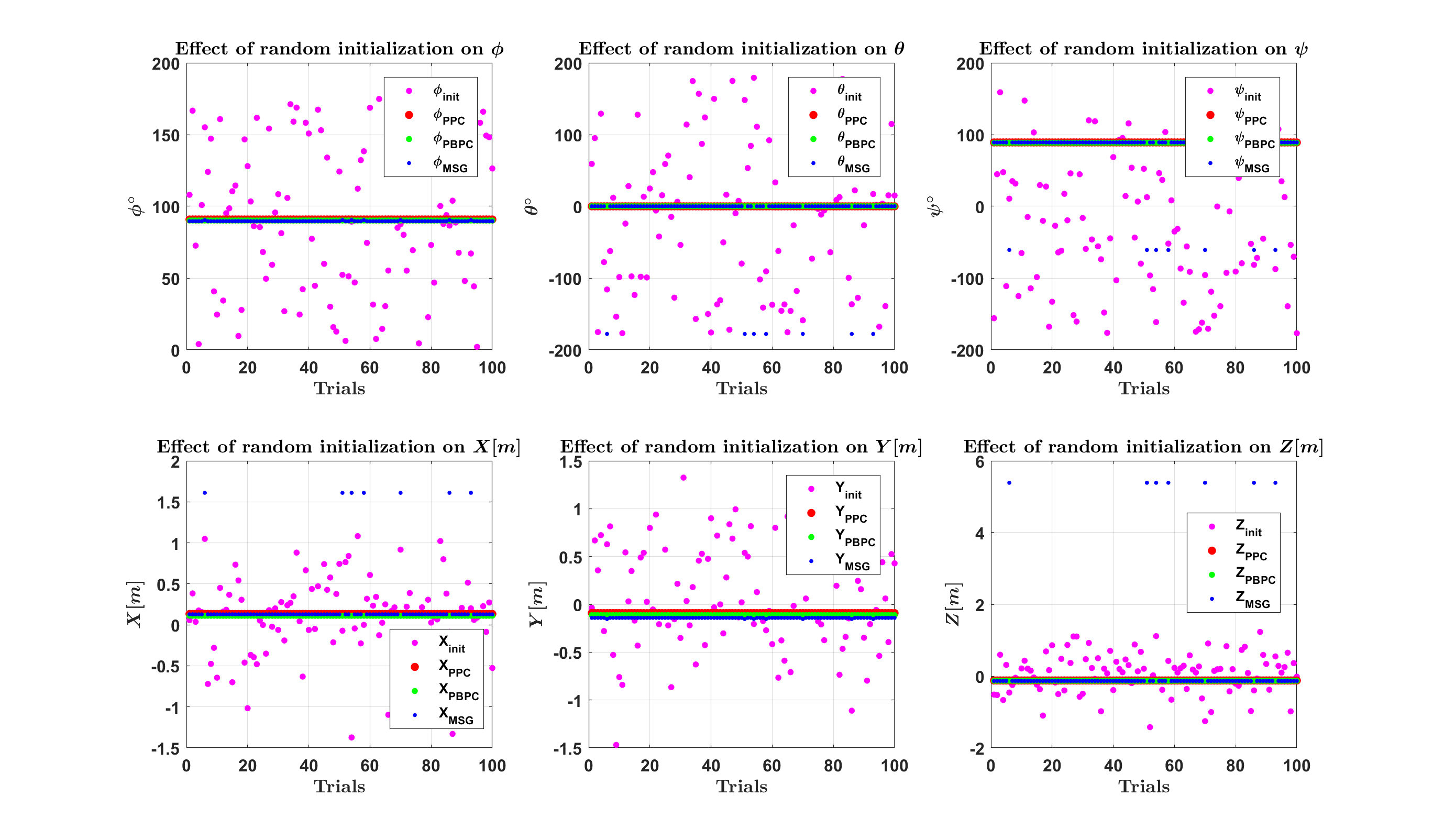
Figure 4: Comparing performance of PPC-Cal, PBPC-Cal and MSG-Cal to random initialization. This figure shows the calibration result for the left stereo camera and Velodyne VLP-32 LIDAR under random initialization

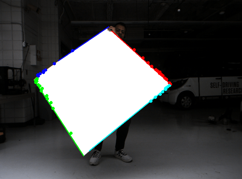
(a) MLRE = 2.94664 with PPC-Cal for VLP-32 and Right Stereo Camera

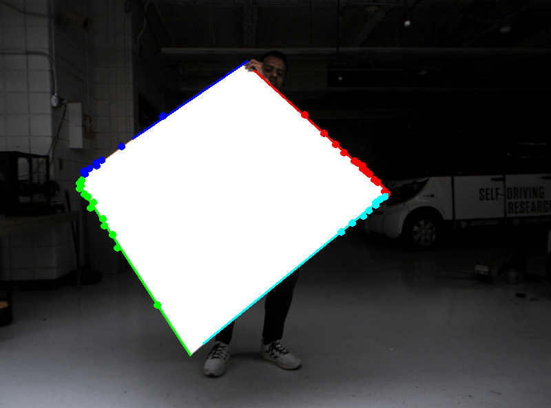
(b) MLRE = 1.88719 with PBPC-Cal for VLP-32 and Right Stereo Camera

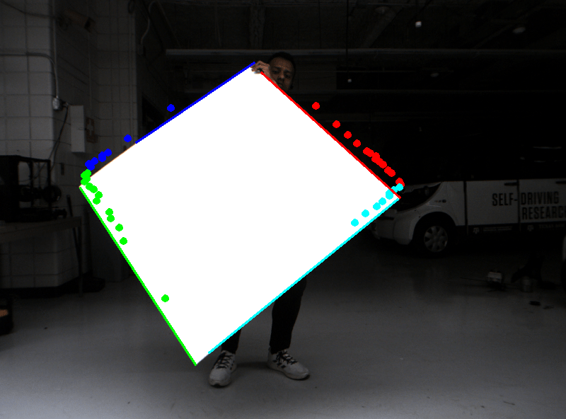
(c) MLRE = 11.3415 with MSG-Cal for VLP-32 and Right Stereo Camera

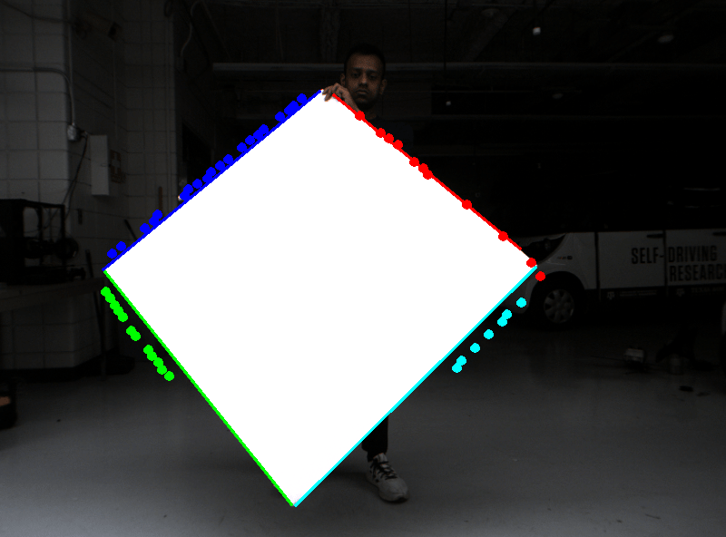
(d) MLRE = 5.63206 with PPC-Cal for OS1-64 and Right Stereo Camera

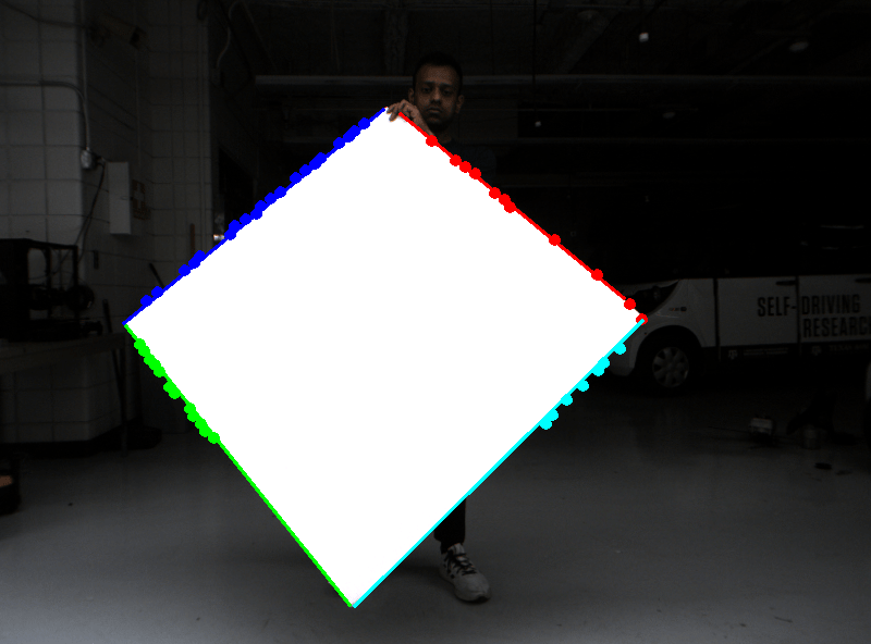
(e) MLRE = 1.74138 with PBPC-Cal for OS1-64 and Right Stereo Camera

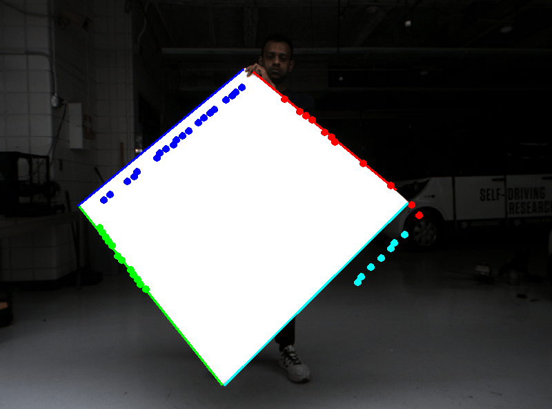
(f) MLRE = 11.0735 with MSG-Cal for OS1-64 and Right Stereo Camera

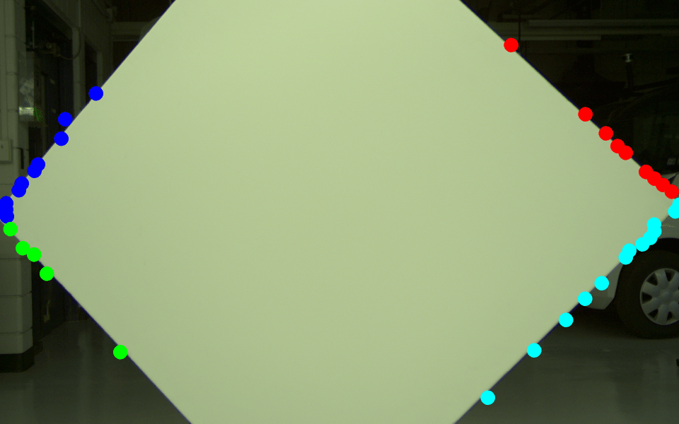
(g) MLRE = 2.21383 with PPC-Cal for VLP-32 and Basler Ace Camera

(h) MLRE = 1.9423 with PBPC-Cal for VLP-32 and Basler Ace Camera

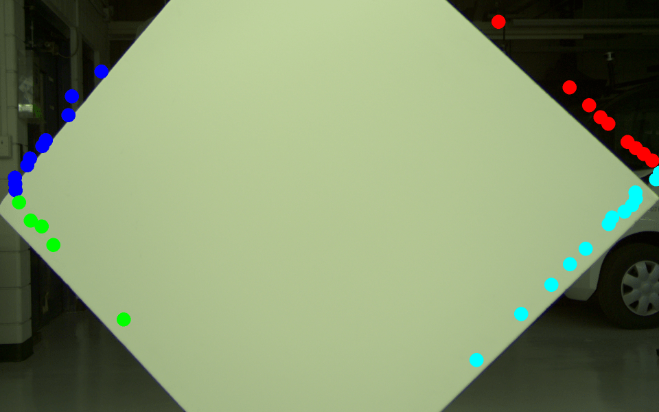
(i) MLRE = 8.8254 with MSG-Cal for VLP-32 and Basler Ace Camera

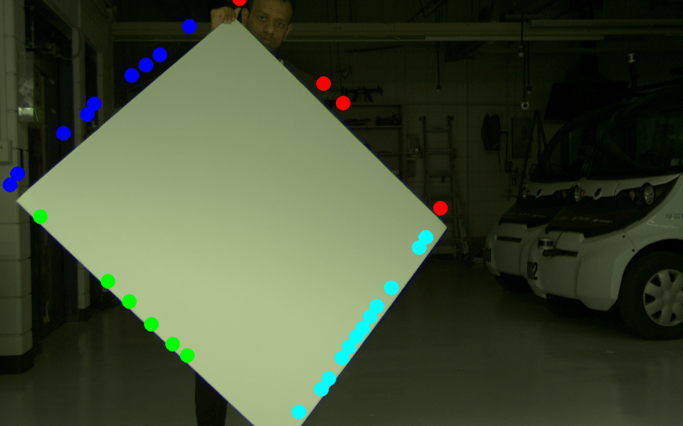
(j) MLRE = 6.95193 with PPC-Cal for OS1-64 and Basler Ace Camera

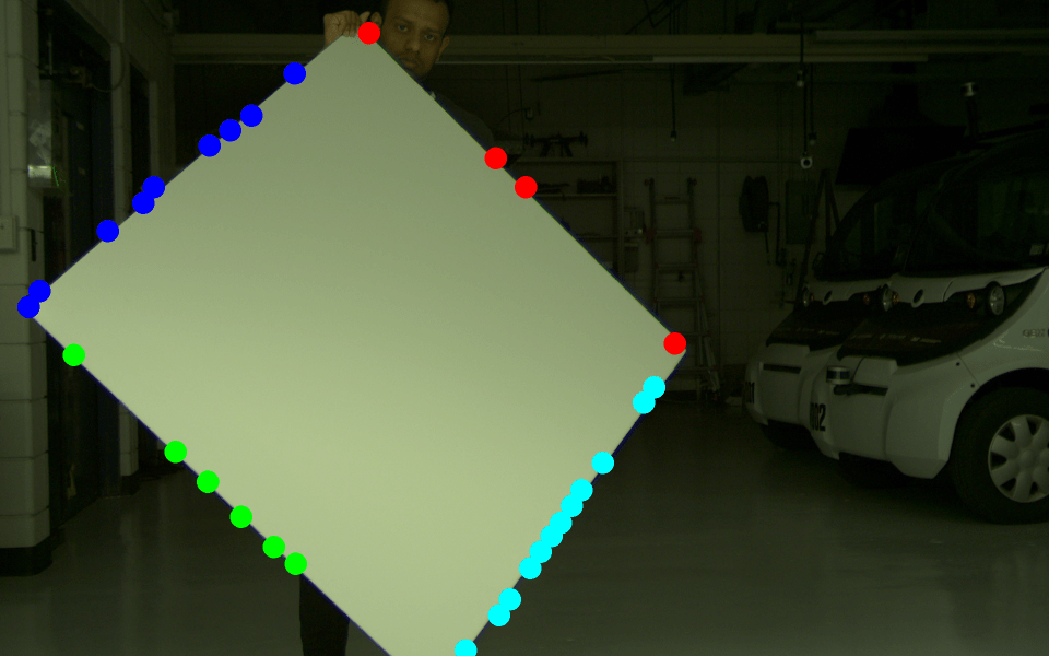
(k) MLRE = 1.80414 with PBPC-Cal for OS1-64 and Basler Ace Camera

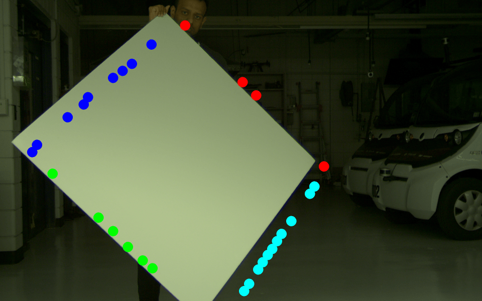
(l) MLRE = 11.7995 with MSG-Cal for OS1-64 and Basler Ace Camera

Figure 5: Comparing performance of PPC-Cal, PBPC-Cal and MSG-Cal using Mean Line Re-projection Error

We compare the performance of PPC-Cal, PBPC-Cal and MSG-Cal by using these methods to calibrate our sensor suite (Figure 2). First, we evaluate their robustness to random initial conditions (Figure 4) drawn from a zero mean normal distribution with standard deviation of $90^{\circ}$ and $50$ cm for rotation and translation respectively. We notice that PPC-Cal and PBPC-Cal are robust to initialization while MSG-Cal exhibits divergence in a few cases, in which the optimization arrives at the same incorrect local minima. Besides, we notice that all the methods converge to nearly the same rotational values but show variation in translation values. This is because the point to plane constraint (which is used in all the three methods) is good at constraining rotation but it needs several observations to constrain translation. The point to back-projected plane constraint (used in PBPC-Cal) helps translation estimation accuracy by providing additional constraints at each measurement. While we don’t expect such bad initial guesses in practice (and initial guesses of Identity converged for each algorithm across multiple datasets), we are effectively showing how well each formulation constrains the optimization. Since the minimization problem(s) (Equation 4, 7, 12) solved to estimate $[^{C}R_{L},^{C}t_{L}]$ are highly non-linear and involve parameters on manifolds, the convergence over several random initialization assures the user that the calibration process can be executed with any initial guess.

In the absence of ground truth we verify our algorithms by using the estimated parameters a) to compare it against the factory stereo calibration and b) to project points lying on the edges of the planar target in LIDAR frame on the Camera image and calculate the mean line re-projection errors (MLRE). MLRE is an independent evaluation metric since none of the methods we compare in this work use it as a residual in their respective optimizations.

	PPC-Cal	PBPC-Cal	MSG-Cal
$\alpha^{\circ}_{err}$	-0.0055535	0.19277	0.10103
$\beta^{\circ}_{err}$	0.097271	0.19995	0.057334
$\gamma^{\circ}_{err}$	-0.081701	-0.12867	-0.11242
$X_{err}$ $[m]$	0.00304	0.00640	-0.00113
$Y_{err}$ $[m]$	-0.00439	-0.00352	-0.00377
$Z_{err}$ $[m]$	0.01124	0.00459	0.01072

TABLE I: Errors with respect to factory stereo calibration for Velodyne VLP-32 LIDAR and the stereo rig.

Errors with respect to factory stereo calibration
	PPC-Cal	PBPC-Cal	MSG-Cal
$\alpha^{\circ}_{err}$	0.51756	0.068189	0.10103
$\beta^{\circ}_{err}$	0.037753	0.12717	0.057334
$\gamma^{\circ}_{err}$	-0.061076	-0.22650	-0.11242
$X_{err}$ $[m]$	-0.00101	-0.00507	-0.00113
$Y_{err}$ $[m]$	-0.00102	-0.00622	-0.00377
$Z_{err}$ $[m]$	0.00877	0.00475	0.01072

TABLE II: Errors with respect to factory stereo calibration for Ouster 64 Channel LIDAR and the stereo rig

3D-LIDAR Camera Pair	MLRE
	PPC-Cal	PBPC-Cal	MSG-Cal
VLP-32 $\leftrightarrow$ Stereo Left	2.57316	1.94707	11.6547
VLP-32 $\leftrightarrow$ Stereo Right	2.94664	1.88719	11.3415
OS1 $\leftrightarrow$ Stereo Left	5.51552	1.76985	10.3954
OS1 $\leftrightarrow$ Stereo Right	5.63206	1.74138	11.0735
VLP-32 $\leftrightarrow$ Basler	2.21383	1.9423	8.8254
OS1 $\leftrightarrow$ Basler	6.95193	1.80414	11.7995
Standard Deviation	1.9723	0.089039	1.1087

TABLE III: MLRE (in pixels) for various 3D-LIDAR Camera Pairs with PPC-Cal, PBPC-Cal and MSG-Cal

In Table I we can see that PPC-Cal and MSG-Cal show error in the order of 1 cm along the stereo baseline dimension (Z axis) as compared to 4.5 mm in PBPC-Cal. In Table II, PPC-Cal shows better performance than the others. We can see that MSG-Cal gives the same error in both the Tables I & II. It is so because MSG-Cal is a graph based approach which does joint optimization of all the sensors together and also does camera$\leftrightarrow$camera pair-wise calibration. It is difficult to draw definitive conclusions by comparing only the stereo errors. Hence, we proceed to compare the MLRE in Table III and Figure 5.

From Table III it can be concluded that the PBPC-Cal performs best among all the three methods. If we compare PPC-Cal and PBPC-Cal we can see that the result of PBPC-Cal is consistent for all the sensor pairs, as expressed by a low standard deviation (0.089039 pixels) but PPC-Cal greater variation as evident from a high standard deviation (1.9723 pixels). As discussed in [17], the Ouster LIDAR is a noisy sensor and PPC-Cal doesn’t perform well when the Ouster Lidar is used. MSG-Cal produced consistent results when using various M-estimators such as Huber and Tukey cost functions, as well as testing various confidence parameters of the Ouster sensor. The confidence value of a sensor propagates to both the pair-wise and global calibration steps. For a pair-wise calibration, the RANSAC inlier threshold is scaled according to the inverse sum of each sensor’s confidence, so that a more permissive threshold is provided for noisier sensors. For the graph calibration, the uncertainty associated with observations from noisier sensors is increased exponentially compared to more accurate sensors. We can hypothesize that the graph based approach MSG-Cal which does joint optimization will have all its nodes affected by Ouster’s noise and therefore gives poor performance as evident from a high reprojection error for all sensor pairs (Table III). To prove our hypothesis we re-calibrate our sensors using MSG-Cal but with the Ouster LIDAR removed and the results are presented in Table IV and Figure 6.

3D-LIDAR Camera Pair	MLRE
	PPC-Cal	PBPC-Cal	MSG-Cal
VLP-32 $\leftrightarrow$ Stereo Left	2.57316	1.94707	3.25161
VLP-32 $\leftrightarrow$ Stereo Right	2.94664	1.88719	2.77772
VLP-32 $\leftrightarrow$ Basler	2.21383	1.9423	2.5893

TABLE IV: MLRE (in pixels) for various 3D-LIDAR Camera Pairs with PPC-Cal, PBPC-Cal and MSG-Cal without Ouster OS1 64 LIDAR

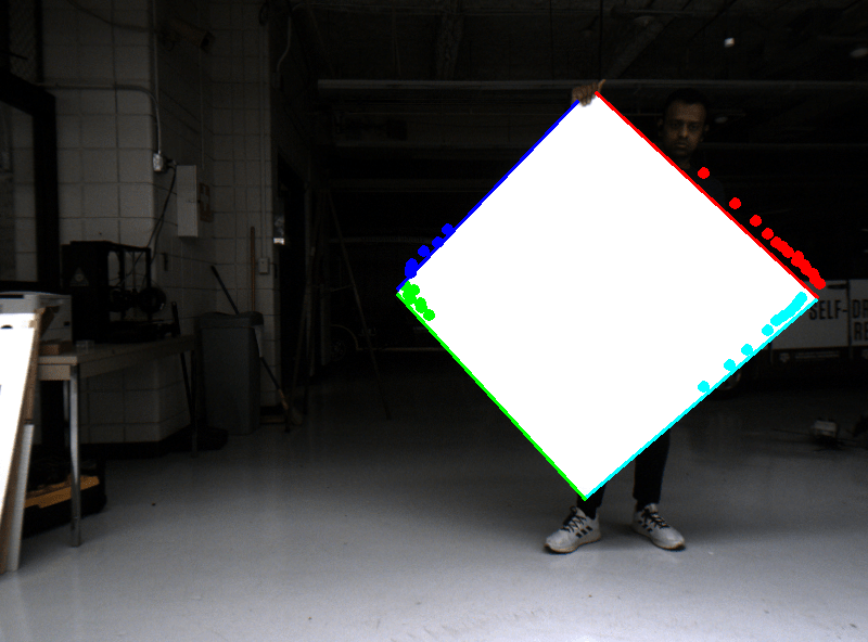
(a) MLRE = 11.6547 with Ouster Lidar in the sensor suite for VLP-32 and Left Stereo Camera

(b) MLRE = 11.3415 with Ouster Lidar in the sensor suite for VLP-32 and Right Stereo Camera

(c) MLRE = 8.8254 with Ouster Lidar in the sensor suite for VLP-32 and Basler Ace Camera

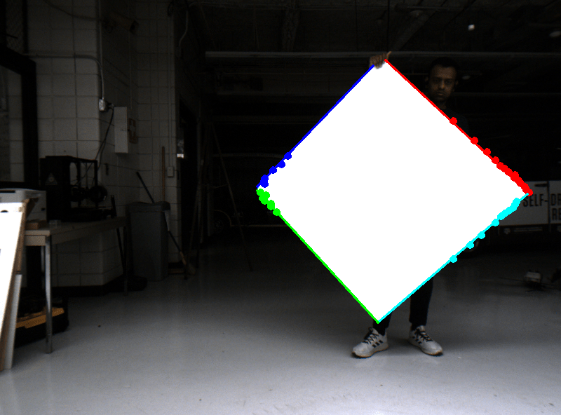
(d) MLRE = 3.25161 without Ouster Lidar in the sensor suite for VLP-32 and Left Stereo Camera

(e) MLRE = 2.77772 without Ouster Lidar in the sensor suite for VLP-32 and Right Stereo Camera

(f) MLRE = 2.5893 without Ouster Lidar in the sensor suite for VLP-32 and Basler Ace Camera

Figure 6: Comparing performance of MSG-Cal with (Figure 6a, Figure 6b, Figure 6c) and without (Figure 6d, Figure 6e, Figure 6f) Ouster LIDAR in the sensor suite(Figure 2)

From Figure 6 we can conclude that MSG-Cal shows significant improvement when used in the absence of Ouster LIDAR and Table IV conveys that without the Ouster in the graph optimization framework, the results of MSG-Cal are similar to those of PPC-Cal which makes sense because the pair-wise calibration in MSG-Cal uses similar constraints as PPC-Cal. Irrespective of Ouster LIDAR’s presence or absence, PBPC-Cal performs the best.

VI Discussion

In this work we compared three LIDAR Camera extrinsic calibration algorithms viz. PPC-Cal ([1], [2] & [3]), PBPC-Cal [17] and MSG-Cal [19]. We presented the mathematical framework behind the working of all these methods and extensively evaluated them on a multi-sensor platform comprising 3 distinct cameras and 2 LIDARs. We concluded that PPC-Cal & PBPC-Cal were robust to random initialization for all trials while MSG-Cal diverged in a few trials (Figure 4). Nevertheless, barring a few cases in MSG-Cal, all the three frameworks can be initialized with any intial condition and will still converge. We showed that the PPC-Cal which uses only point to plane constraint shows deterioration in performance when a noisy sensor is used (Table III). The use of additional point to back-projected plane constraint in PBPC-Cal helps reduce the effect of noisy sensor by introducing more geometrical constraints to the non-linear cost function. We also showed that the global graph based optimization method MSG-Cal, which uses a variant of the point to plane constraint has all final pair wise calibrations (as evident from high MLRE from Table III) affected in the presence of a noisy sensor but gives comparable performance to PPC-Cal when the noisy sensor is removed (Table IV). PBPC-Cal exhibits similar performance both with and without the noisy sensor and performs better than both PPC-Cal and MSG-Cal under all circumstances (Tables III & IV, Figure 5). If we do not have a noisy sensor and need a quick calibration result then using PPC-Cal is a good option but if we have multiple sensors (with low noise) then MSG-Cal should be the algorithm of choice, as collecting data for both these methods is easier. Instead, if we have noisy sensors then PBPC-Cal should be used. In the future we want to use PBPC-Cal in the pair-wise calibration step of MSG-Cal, thus bringing the benefits of robust pair-wise calibration and joint global optimization together.

VII Acknowledgements

The authors would like to thank Peng Jiang for his invaluable help with data collection.

References

- [1] R. Unnikrishnan and M. Hebert, “Fast extrinsic calibration of a laserrangefinder to a camera,” 07 2005.
- [2] L. Huang and M. Barth, “A novel multi-planar lidar and computer vision calibration procedure using 2d patterns for automated navigation,” in 2009 IEEE Intelligent Vehicles Symposium, June 2009, pp. 117–122.
- [3] G. Pandey, J. McBride, S. Savarese, and R. Eustice, “Extrinsic calibration of a 3d laser scanner and an omnidirectional camera,” IFAC Proceedings Volumes, vol. 43, no. 16, pp. 336 – 341, 2010, 7th IFAC Symposium on Intelligent Autonomous Vehicles. [Online]. Available: http://www.sciencedirect.com/science/article/pii/S1474667016350790
- [4] L. Zhou and Z. Deng, “Extrinsic calibration of a camera and a lidar based on decoupling the rotation from the translation,” 06 2012, pp. 642–648.
- [5] L. Zhou, Z. Li, and M. Kaess, “Automatic extrinsic calibration of a camera and a 3d lidar using line and plane correspondences,” 10 2018, pp. 5562–5569.
- [6] G. Pandey, J. McBride, S. Savarese, and R. Eustice, “Automatic extrinsic calibration of vision and lidar by maximizing mutual information,” Journal of Field Robotics, vol. 32, 09 2014.
- [7] J. Levinson and S. Thrun, “Automatic online calibration of cameras and lasers,” 06 2013.
- [8] D. Scaramuzza, A. Harati, and R. Siegwart, “Extrinsic self calibration of a camera and a 3d laser range finder from natural scenes,” in 2007 IEEE/RSJ International Conference on Intelligent Robots and Systems, Oct 2007, pp. 4164–4169.
- [9] Z. Taylor and J. Nieto, “Motion-based calibration of multimodal sensor extrinsics and timing offset estimation,” IEEE Transactions on Robotics, vol. 32, no. 5, pp. 1215–1229, Oct 2016.
- [10] S. Wasielewski and O. Strauss, “Calibration of a multi-sensor system laser rangefinder/camera,” in Proceedings of the Intelligent Vehicles ’95. Symposium, Sep. 1995, pp. 472–477.
- [11] Qilong Zhang and R. Pless, “Extrinsic calibration of a camera and laser range finder (improves camera calibration),” in 2004 IEEE/RSJ International Conference on Intelligent Robots and Systems (IROS) (IEEE Cat. No.04CH37566), vol. 3, Sep. 2004, pp. 2301–2306 vol.3.
- [12] R. Gomez-Ojeda, J. Briales, E. Fernandez-Moral, and J. Gonzalez-Jimenez, “Extrinsic calibration of a 2d laser-rangefinder and a camera based on scene corners,” in 2015 IEEE International Conference on Robotics and Automation (ICRA), May 2015, pp. 3611–3616.
- [13] O. Naroditsky, A. Patterson, and K. Daniilidis, “Automatic alignment of a camera with a line scan lidar system,” in 2011 IEEE International Conference on Robotics and Automation, May 2011, pp. 3429–3434.
- [14] S. A. Rodriguez F., V. Fremont, and P. Bonnifait, “Extrinsic calibration between a multi-layer lidar and a camera,” in 2008 IEEE International Conference on Multisensor Fusion and Integration for Intelligent Systems, Aug 2008, pp. 214–219.
- [15] M. Velas, M. Spanel, Z. Materna, and A. Herout, “Calibration of rgb camera with velodyne lidar.”
- [16] A. Geiger, F. Moosmann, O. Car, and B. Schuster, “Automatic camera and range sensor calibration using a single shot,” Proceedings - IEEE International Conference on Robotics and Automation, pp. 3936–3943, 05 2012.
- [17] S. Mishra, G. Pandey, and S. Saripalli, “Extrinsic calibration of a 3d-lidar and a camera,” Submitted to IV2020, 02 2020.
- [18] Q. V. Le and A. Y. Ng, “Joint calibration of multiple sensors,” in 2009 IEEE/RSJ International Conference on Intelligent Robots and Systems, Oct 2009, pp. 3651–3658.
- [19] J. L. Owens, P. R. Osteen, E. Corporation, and K. Daniilidis, “Msg-cal: Multi-sensor graph-based calibration.”
- [20] S. Garrido-Jurado, R. Muñoz Salinas, F. Madrid-Cuevas, and R. Medina-Carnicer, “Generation of fiducial marker dictionaries using mixed integer linear programming,” Pattern Recognition, vol. 51, 10 2015.
- [21] E. Olson, “AprilTag: A robust and flexible visual fiducial system,” in Proceedings of the IEEE International Conference on Robotics and Automation (ICRA). IEEE, May 2011, pp. 3400–3407.
- [22] J. Kümmerle, T. Kühner, and M. Lauer, “Automatic calibration of multiple cameras and depth sensors with a spherical target,” in 2018 IEEE/RSJ International Conference on Intelligent Robots and Systems (IROS), Oct 2018, pp. 1–8.
- [23] Z. Zhang, “A flexible new technique for camera calibration,” IEEE Trans. Pattern Anal. Mach. Intell., vol. 22, no. 11, p. 1330–1334, Nov. 2000. [Online]. Available: https://doi.org/10.1109/34.888718
- [24] R. Hartley and A. Zisserman, Multiple View Geometry in Computer Vision, 2nd ed. New York, NY, USA: Cambridge University Press, 2003.
- [25] M. A. Fischler and R. C. Bolles, “Random sample consensus: A paradigm for model fitting with applications to image analysis and automated cartography,” Commun. ACM, vol. 24, no. 6, pp. 381–395, Jun. 1981. [Online]. Available: http://doi.acm.org/10.1145/358669.358692
- [26] R. B. Rusu and S. Cousins, “3d is here: Point cloud library (pcl),” in 2011 IEEE International Conference on Robotics and Automation, May 2011, pp. 1–4.
- [27] G. Bradski, “The OpenCV Library,” Dr. Dobb’s Journal of Software Tools, 2000.
- [28] S. Agarwal, K. Mierle, and Others, “Ceres solver,” http://ceres-solver.org.
- [29] R. Grompone von Gioi, J. Jakubowicz, J. Morel, and G. Randall, “Lsd: A fast line segment detector with a false detection control,” IEEE Transactions on Pattern Analysis and Machine Intelligence, vol. 32, no. 4, pp. 722–732, April 2010.
- [30] B. Pribyl, P. Zemcík, and M. Cadík, “Pose estimation from line correspondences using direct linear transformation,” CoRR, vol. abs/1608.06891, 2016. [Online]. Available: http://arxiv.org/abs/1608.06891
- [31] R. Kümmerle, G. Grisetti, H. Strasdat, K. Konolige, and W. Burgard, “G2o: A general framework for graph optimization,” 06 2011, pp. 3607 – 3613.