Probing Dark Low-mass Halos and Primordial Black Holes with Frequency-dependent Gravitational Lensing Dispersions of Gravitational Waves

Abstract

We explore the possibility of using amplitude and phase fluctuations of gravitational waves due to gravitational lensing as a probe of the small-scale matter power spectrum. The direct measurement of the small-scale matter power spectrum is made possible by making use of the frequency dependence of such gravitational lensing dispersions originating from the wave optics nature of the propagation of gravitational waves. We first study the small-scale behavior of the matter power spectrum in detail taking the so-called halo model approach including effects of baryons and subhalos. We find that the matter power spectrum at the wavenumber $k\sim 10^{6}h{\rm Mpc}^{-1}$ is mainly determined by the abundance of dark low-mass halos with mass $1h^{-1}M_{\odot}\lesssim M\lesssim 10^{4}h^{-1}M_{\odot}$ and is relatively insensitive to baryonic effects. The matter power spectrum at this wavenumber is probed by gravitational lensing dispersions of gravitational waves at frequencies of $f\sim 0.1-1$ Hz with predicted signals of $\mathcal{O}(10^{-3})$. We also find that primordial black holes (PBHs) with $M_{\rm PBH}\gtrsim 0.1\leavevmode\nobreak\ M_{\odot}$ can significantly enhance the matter power spectrum at $k\gtrsim 10^{5}h{\rm Mpc}^{-1}$ due to both the enhanced halo formation and the shot noise from PBHs. We find that gravitational lensing dispersions at $f\sim 10-100$ Hz are particularly sensitive to PBHs and can be enhanced by more than an order of magnitude depending on the mass and abundance of PBHs.

1 Introduction

The nature of dark matter remains one of the central problems in cosmology. While the cold dark matter (CDM) model (Peebles, 1982; Blumenthal et al., 1984; Davis et al., 1985) is successful in explaining a variety of cosmological observations including the cosmic microwave background (Planck Collaboration et al., 2016) and the large-scale structure of the Universe (Alam et al., 2017), there are several competing candidates of cold dark matter, including weakly interacting massive particles, ultra-light dark matter, and primordial black holes (see e.g., Battaglieri et al., 2017). A number of experiments are ongoing and planned to detect dark matter and to discriminate these different candidates.

Cosmological and astrophysical observations provide an important means of studying the property of dark matter particles, because different dark matter candidates can predict quite different small-scale distributions of dark matter. In observations, there have been debates about the validity of the simplest collisionless CDM model at the dwarf galaxy scale. For example, core-like radial density profiles of many dark-matter dominated dwarf galaxies and the small number of satellite dwarf galaxies in the Milky Way and the Local Group (see Bullock & Boylan-Kolchin, 2017, for a review) may hint the particle nature of dark matter, although it has been argued that the modification of dark matter distributions by complex baryon physics such as star formation and supernova feedback may well explain the observed properties of dwarf galaxies even in the context of the simplest collisionless CDM model.

One way to settle the debate is to study dark low-mass halos. Since the galaxy formation theory predicts that halos with masses $\lesssim 10^{7}M_{\odot}$ contain very little or no star, properties of such dark low-mass halos are barely affected by the complex baryon physics, which makes them an ideal site for testing various dark matter candidates. However, detecting such dark low-mass halos is quite challenging. Several ideas include flux ratio anomalies in gravitationally lensed quasars (e.g., Mao & Schneider, 1998; Inoue et al., 2015; Gilman et al., 2020), perturbations in galaxy-galaxy strong lensing (e.g., Inoue & Chiba, 2003; Koopmans, 2005; Vegetti et al., 2012; Ritondale et al., 2019), perturbations in stellar streams in the Milky Way (e.g., Ibata et al., 2002; Bovy et al., 2017; Banik et al., 2019), pulsar timing array (e.g., Kashiyama & Oguri, 2018; Dror et al., 2019), astrometric weak gravitational lensing (e.g., Van Tilburg et al., 2018; Mondino et al., 2020), caustic crossings in massive clusters (e.g., Kelly et al., 2018; Dai et al., 2018b; Dai & Miralda-Escudé, 2020), and diffraction effects in gravitational lensing (e.g., Dai et al., 2018a). Some of these techniques already place interesting constraints on the abundance of low-mass halos down to $\sim 10^{8}M_{\odot}$ that is roughly consistent with the standard CDM prediction. Thus pushing such constraints to even lower halo masses is anticipated.

One of the candidates of CDM includes Primordial Black Holes (PBHs) that formed in the early Universe (see e.g., Sasaki et al., 2018; Carr et al., 2020, for reviews). The PBH dark matter scenario has attracted a lot of attention given the discovery of gravitational waves from a binary black hole merger (Abbott et al., 2016). The abundance of PBHs around the mass scale of such binary black hole mergers has been constrained by e.g., quasar microlensing (Mediavilla et al., 2017), caustic crossings (Oguri et al., 2018), and gravitational lensing of Type Ia supernovae (Zumalacárregui & Seljak, 2018). Tighter constraints on their abundance are needed to check whether PBHs can account for observed gravitational wave events.

In this paper, we explore the possibility of using gravitational lensing dispersions of gravitational waves as a new probe of dark low-mass halos and PBHs. The gravitational lensing dispersion refers to the dispersion of the brightness of a distant source due to gravitational lensing (de)magnification caused by intervening matter along the line-of-sight. Such gravitational lensing dispersions have been detected from samples of Type Ia supernovae (Jönsson et al., 2007, 2010; Kronborg et al., 2010; Karpenka et al., 2013; Smith et al., 2014), and contain information on the matter power spectrum at small scales (Bernardeau et al., 1997; Metcalf, 1999; Hamana & Futamase, 2000; Dodelson & Vallinotto, 2006; Quartin et al., 2014; Fedeli & Moscardini, 2014; Ben-Dayan & Kalaydzhyan, 2014; Ben-Dayan & Takahashi, 2016; Hada & Futamase, 2016, 2019; Agrawal et al., 2019).

This approach can easily be extended to gravitational waves from compact binary mergers given their standard siren nature (Schutz, 1986; Holz & Hughes, 2005). A notable difference of gravitational lensing of gravitational waves from that of supernovae is that wave optics effects can play an important role in some situations (see e.g., Nakamura & Deguchi, 1999; Oguri, 2019, for reviews). For instance, gravitational lensing magnifications are significantly suppressed due to diffraction when the wavelength of gravitational waves is larger than the Schwarzschild radius of the lens. In the case of gravitational lensing dispersions, density fluctuations below the so-called Fresnel scale, which depends on the frequency of gravitational waves, do not contribute to the dispersion due to diffraction (Macquart, 2004; Takahashi et al., 2005; Takahashi, 2006). Taking advantage of this effect, Takahashi (2006) proposed to use amplitude and phase changes as a function of the frequency of gravitational waves to probe the matter power spectrum at the Fresnel scales. In this paper we extend this idea and explore the detectability of dark low-mass halos and primordial black holes with frequency dependent gravitational lensing dispersions of gravitational waves. For this purpose, we study the behavior of the matter power spectrum at very small scales ($k\gg 1$ Mpc^-1) in detail, including the modification of the power spectrum due to baryon physics, taking the halo model approach.

This paper is organized as follows. We present our halo model including effects of baryons and subhalos in Section 2. We then present results of gravitational lensing dispersions of gravitational waves in Section 3. Some discussions are given in Section 4. Finally we conclude in Section 5. Throughout the paper we adopt the $\Lambda$-dominated CDM model with the matter density $\Omega_{\rm m}=0.3089$, the baryon density $\Omega_{\rm b}=0.0486$, the cosmological constant $\Omega_{\Lambda}=0.6911$, the dimensionless Hubble constant $h=0.6774$, the spectral index $n_{\rm s}=0.9667$, and the normalization of the density fluctuation $\sigma_{8}=0.8159$, which are cosmological parameters adopted in the IllustrisTNG cosmological hydrodynamical simulations (Nelson et al., 2018; Springel et al., 2018; Pillepich et al., 2018; Marinacci et al., 2018; Naiman et al., 2018). Throughout the paper we always assume a flat Universe for calculating distances.

2 Halo Model

2.1 Standard Calculation

The halo model (see e.g., Cooray & Sheth, 2002, for a review) provides a powerful means of studying nonlinear gravitational clustering. It assumes that all the matter is confined in dark matter halos. With this assumption, the matter density field $\rho(\boldsymbol{x})$ is written as

$$\rho(\boldsymbol{x})=\sum_{i}M_{i}u\left(\boldsymbol{x}-\boldsymbol{x}_{i}|M_{i}\right),$$ (1)

where $i$ labels dark matter halos, $M_{i}$ and $\boldsymbol{x}_{i}$ are the mass and the spatial position of $i$-th halo, and $u(\boldsymbol{x}|m)$ denotes the normalized density profile of a halo with mass $M$ that satisfies $\int d\boldsymbol{x}\,u(\boldsymbol{x}|M)=1$. Usually the Navarro et al. (1997, hereafter NFW) density profile is adopted as the density profile of each halo. From Equation (1), it is found that the matter power spectrum is described by the sum of the so-called 1-halo and 2-halo terms (see Appendix A for the derivation)

$$P(k)=P^{\rm 1h}(k)+P^{\rm 2h}(k),$$ (2)

$$P^{\rm 1h}(k)=\int dM\frac{dn}{dM}\left(\frac{M}{\bar{\rho}}\right)^{2}u^{2}(k|M),$$ (3)

$$P^{\rm 2h}(k)=\left[\int dM\frac{dn}{dM}\left(\frac{M}{\bar{\rho}}\right)b(M)\,u(k|M)\right]^{2}P_{\rm lin}(k),$$ (4)

where $dn/dM$ denotes the halo mass function, $\bar{\rho}$ is the mean comoving matter density, $u(k|M)$ is the Fourier transform of the normalized density profile, $b(M)$ is a linear halo bias, and $P_{\rm lin}(k)$ is the linear matter power spectrum.

2.2 Modifications of 1-halo Term

The baryon cooling and star formation modify the matter distribution in each halo, and thereby affect the matter power spectrum (see e.g., Chisari et al., 2019, for a review). Such baryonic effects have been studied using the halo model, mostly focusing on their impact on cosmic shear cosmology (e.g., White, 2004; Zhan & Knox, 2004; Semboloni et al., 2011; Fedeli, 2014; Fedeli et al., 2014; Debackere et al., 2020). In addition, substructures or subhalos in dark matter halos may affect the matter power spectrum at very small scales, as studied in Giocoli et al. (2010).

Following the literature, we consider effects of the stellar component and subhalos, both of which can be important at very small scales, and ignore the effect of the gas component. In presence of these components, Equation (1) is rewritten as

$$\rho(\boldsymbol{x})=\sum_{i}M_{i}\left[(1-f_{\rm s})u_{\rm h}\left(\boldsymbol{x}-\boldsymbol{x}_{i}|M_{i}\right)+f_{\rm s}u_{\rm s}\left(\boldsymbol{x}-\boldsymbol{x}_{i}|M_{i}\right)\right],$$ (5)

where

$$u_{\rm h}\left(\boldsymbol{x}-\boldsymbol{x}_{i}|M_{i}\right) = \frac{1-f_{*}-f_{\rm s}}{1-f_{\rm s}}u\left(\boldsymbol{x}-\boldsymbol{x}_{i}|M_{i}\right)$$ (6)

$$+\frac{f_{*}}{1-f_{\rm s}}u_{*}\left(\boldsymbol{x}-\boldsymbol{x}_{i}|M_{i}\right),$$

$$u_{\rm s}\left(\boldsymbol{x}-\boldsymbol{x}_{i}|M_{i}\right)=\frac{1}{f_{\rm s}M_{i}}\sum_{j}m_{j}u_{\rm sub}(\boldsymbol{x}-\boldsymbol{x}_{j}|M_{i},m_{j},\boldsymbol{x}_{j}-\boldsymbol{x}_{i}),$$ (7)

$f_{*}$ and $f_{\rm s}$ are mass fractions of stellar and subhalo components, respectively, $m_{j}$ is the mass of the $j$-th subhalo, and $u_{*}$ and $u_{\rm sub}$ denote normalized density profiles of stellar and subhalo components, respectively. For simplicity, throughout the paper we ignore the dependence of $u_{\rm sub}$ on the position within a halo by setting $u_{\rm sub}(\boldsymbol{x}-\boldsymbol{x}_{j}|M_{i},m_{j},\boldsymbol{x}_{j}-\boldsymbol{x}_{i})=u_{\rm sub}(\boldsymbol{x}-\boldsymbol{x}_{j}|M_{i},m_{j})$. Repeating the similar calculation as done for the standard halo model case (see Appendix A), we obtain

$$P^{\rm 1h}(k)=P^{\rm 1h,hh}(k)+P^{\rm 1h,hs}(k)+P^{\rm 1h,ss}(k),$$ (8)

$$P^{\rm 1h,hh}(k)=\int dM\frac{dn}{dM}\left(\frac{M}{\bar{\rho}}\right)^{2}(1-f_{\rm s})^{2}u_{\rm h}^{2}(k|M),$$ (9)

$$P^{\rm 1h,hs}(k)=\int dM\frac{dn}{dM}\left(\frac{M}{\bar{\rho}}\right)^{2}2(1-f_{\rm s})u_{\rm h}(k|M)I(k|M),$$ (10)

$$P^{\rm 1h,ss}(k)=\int dM\frac{dn}{dM}\left(\frac{M}{\bar{\rho}}\right)^{2}\left[I^{2}(k|M)+J(k|M)\right],$$ (11)

where

$$I(k|M)=\int dm\frac{dN_{M}}{dm}\left(\frac{m}{M}\right)u_{\rm sub}(k|M,m)U(k|M,m),$$ (12)

$$J(k|M)=\int dm\frac{dN_{M}}{dm}\left(\frac{m}{M}\right)^{2}u^{2}_{\rm sub}(k|M,m),\\$$

$dN_{M}/dm$ is the subhalo mass function within a halo with mass $M$ and $U(k|M)$ is the Fourier transform of the spatial distribution of subhalos $U(\boldsymbol{x}|M,m)$.

The stellar component $u_{*}$ actually consists of stars, which indicates that the shot noise due to the discrete nature of the stellar component may be important at very small scales. Following the calculation in Appendix A, we include the shot noise from stars by replacing $u_{*}^{2}(k|M)$ to

$$u_{*}^{2}(k|M)\rightarrow u_{*}^{2}(k|M)+\frac{1}{N_{*}},$$ (13)

where $N_{*}=f_{*}M/m_{\rm star}$ denotes the total number of stars in each halo with mass $M$ and $m_{\rm star}$ is the mass of each star. Here we assume that all stars share the same mass for simplicity.

It is instructive to approximate the expressions above further to understand their behavior. Simulations suggest that the spatial distribution of subhalos approximately follows that of the smooth matter component. If we simply assume $U(k|M,m)\approx u_{\rm h}(k|M)$, and use the fact that $u_{\rm sub}(k|M,m)\sim 1$ when $U(k|M,m)$ takes large values, we obtain $I(k|M)\approx f_{\rm s}u_{\rm h}(k|M)$. Under this approximation the 1-halo power spectrum is further simplified as

$$P^{\rm 1h}(k)\approx\int dM\frac{dn}{dM}\left(\frac{M}{\bar{\rho}}\right)^{2}\left[u_{\rm h}^{2}(k|M)+J(k|M)\right],$$ (14)

where the first term of the right hand side of Equation (14) corresponds to the 1-halo power spectrum without any subhalo, and the dominant effect of the subhalo is given by the second term of the right hand side of Equation (14), which represents the auto-correlation of the matter distribution within each subhalo.

2.3 Model Ingredients

We adopt a smoothly truncated NFW profile studied by Baltz et al. (2009, hereafter BMO) for the density profile of main halos. Specifically we adopt the following density profile

$$\rho_{\rm BMO}(r)=\frac{\rho_{\rm s}}{(r/r_{\rm s})(1+r/r_{\rm s})^{2}}\left(\frac{r_{\rm t}^{2}}{r^{2}+r_{\rm t}^{2}}\right)^{2},$$ (15)

which we parametrize by the virial mass $M=M_{\rm vir}$, the concentration parameter $c=c_{\rm vir}=r_{\rm vir}/r_{\rm s}$, and the truncation radius $\tau=r_{\rm t}/r_{\rm s}$. We adopt a fitting form of the mass-concentration relation presented by Diemer & Kravtsov (2015) with updates of fitting parameters by Diemer & Joyce (2019) and the conversion from $c_{\rm 200c}$ to $c_{\rm vir}$ assuming an NFW profile. We then compute $\rho_{\rm s}$ and $r_{\rm s}$ for a given mass and redshift from the mass-concentration relation and in a standard manner assuming the NFW profile (i.e., ignoring the effect of the truncation). We determine $\tau$ such that the total mass of the BMO profile matches $M$ i.e.,

$$f_{\rm BMO}(\tau)=f_{\rm NFW}(c),$$ (16)

$$f_{\rm BMO}(\tau)=\frac{\tau^{2}\left[(3\tau^{2}-1)(\pi\tau-\tau^{2}-1)+2\tau^{2}(\tau^{2}-3)\ln\tau\right]}{2(\tau^{2}+1)^{3}},$$ (17)

$$f_{\rm NFW}(c)=\ln(1+c)-\frac{c}{1+c}.$$ (18)

For typical values of $c$, we obtain $\tau\sim(1.4-1.6)c$ from this condition. The Fourier transform $u(k|M)$ of the normalized BMO profile is given in Appendix B of Oguri & Hamana (2011). The procedure above ensures $u(k|M)\rightarrow 1$ at $k\rightarrow 0$. Since the BMO profile is smoothly truncated, an oscillating feature in $u(k|M)$, which is seen in the Fourier transform of the NFW profile truncated at $r=r_{\rm vir}$ (e.g., Cooray & Sheth, 2002), is suppressed.

For the mass function $dn/dM$ and halo bias $b(M)$, we adopt a model of Sheth & Tormen (1999) that is reasonably accurate for wide mass and redshift ranges.

We need to specify the stellar mass fraction $f_{*}$ and the density profile $\rho_{*}(r)=f_{*}Mu_{*}(r)$ as a function of the halo mass $M$ in order to address baryonic effects. We adopt the stellar mass–halo mass relation for all central galaxies presented by Behroozi et al. (2019) as $f_{*}$. Note that we adopt the mean stellar mass–halo mass relation, which is computed from the median relation in Behroozi et al. (2019) and assuming the log-normal distribution with the scatter of $0.3$ dex. We adopt the Hernquist (1990) profile as the density profile of the stellar component

$$\rho_{*}(r)=\frac{f_{*}M}{2\pi(r/r_{\rm b})(r+r_{\rm b})^{3}},$$ (19)

where $r_{\rm b}$ is related with the effective radius as $r_{\rm b}=0.551r_{\rm e}$. Since it has been shown that galaxy sizes are proportional to virial radii of their host halos for a wide halo mass range (e.g., Kravtsov, 2013; Kawamata et al., 2015; Huang et al., 2017; Kawamata et al., 2018; Kravtsov et al., 2018; Zanisi et al., 2020), in this paper we simply assume

$$r_{\rm e}=0.006r_{\rm vir},$$ (20)

at $z=0$, and it evolves with redshift with $\propto(1+z)^{-1}$ that roughly matches the observed redshift evolution of galaxy sizes. The Fourier transform of the normalized density profile is given by

$$u_{*}(k|M)=1-x{\rm Ci}(x)\sin x-\frac{1}{2}x\left[\pi-2{\rm Si}(x)\right]\cos x,$$ (21)

where $x=kr_{\rm b}(1+z)$ and ${\rm Si}(x)$ and ${\rm Ci}(x)$ are sine and cosine integrals, respectively. The shot noise from stars (equation 13) is computed assuming the star mass of $m_{\rm star}=0.5\leavevmode\nobreak\ M_{\odot}$.

We also need a model of subhalos. We adopt a simple analytic model presented in Appendix B to compute the mass function and the density profile of subhalos. We assume that their radial distribution within each halo follows that of the smooth dark matter distribution i.e., the BMO profile $U(k|M,m)=u(k|M)$. We adopt the BMO profile also for the mass distribution of each subhalo but with different model parameters from those of main halos, as detailed in Appendix B. Similarly to main halos, we consider baryonic effects for subhalos as well using the mean stellar mass–halo mass relation for all satellite galaxies presented by Behroozi et al. (2019). We estimate subhalo masses before tidal stripping $m_{\rm f}$ (see Appendix B for more details) as a proxy of the peak mass in Behroozi et al. (2019) to derive the stellar mass fraction of subhalos, $f_{*}^{\rm s}$. The Fourier transform of the normalized subhalo density profile is given by

$$u_{\rm sub}(k|M,m)=(1-f_{*}^{\rm s})u(k|m,M)+f_{*}^{\rm s}u_{*}(k|m_{\rm ext}),$$ (22)

where $u(k|m,M)$ is the Fourier transform of the normalized BMO profile with total mass $m$, the concentration parameter $c_{\rm sub}$, and truncated at $r_{\rm t}^{\rm ave}$, and $u_{*}(k|m_{\rm ext})$ is given by Equation (21) with $r_{\rm b}$ computed from $m_{\rm f}$.

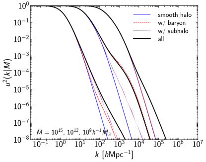
Figure 1: Comparison of the Fourier transform of the halo density profile $u^{2}(k|M)$ at $z=0$ with and without effects of baryon and subhalos. From left to right, we show results for halos with mass $M=10^{15}h^{-1}M_{\odot}$, $10^{12}h^{-1}M_{\odot}$, and $10^{9}h^{-1}M_{\odot}$, respectively. Thin solid lines corresponds to the case with only the smooth main halo, dashed and dotted lines are after adding stellar components and subhalos, respectively, and thick solid lines show the case with both stellar components and subhalos are included. Here the shot noise from stars is not included.

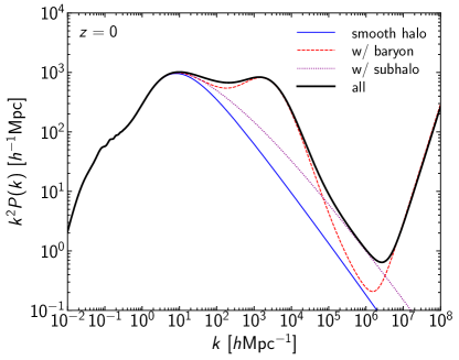
Figure 2: Comparison of matter power spectra $P(k)$ at $z=0$ with and without effects of baryon and subhalos. Lines are same as in Figure 1.

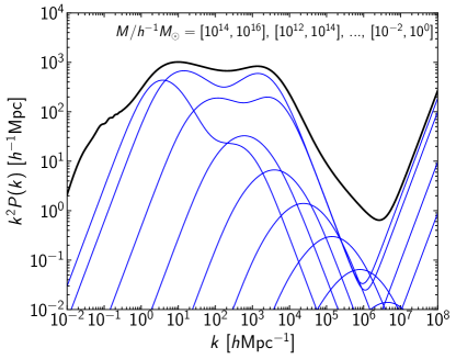
Figure 3: Contributions from halos with different masses to the matter power spectrum $P(k)$ at $z=0$. From left to right thin lines, we show contributions in the 2 dex mass range from higher to lower masses of halos. Here we show contributions from main halos only i.e., without subhalos but including baryonic effects.

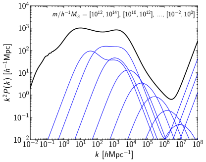
Figure 4: Similar to Figure 3, but contributions from subhalos with different masses are shown. To isolate effects of subhalos, here we include only the $J(k|M)$ term in Equation (11) to compute these contributions.

2.4 Some Examples

Before presenting examples of calculations of matter power spectra, in Figure 1 we show the Fourier transform of the halo density profile with and without effects of baryon and subhalos. The Figure indicates that both subhalos and baryonic stellar components significantly enhance the small scale power of individual halo density profiles. Baryonic effects depend sensitively on the halo mass, reflecting the halo mass dependence of the stellar mass–halo mass relation. While the effects of baryon are more pronounced at $M\sim 10^{12}h^{-1}M_{\odot}$, the effects of subhalos are more significant for very high and low-mass halos.

Figure 2 shows matter power spectra at $z=0$ computed from the halo model presented above. We show $k^{2}P(k)$ because it represents contributions to gravitational lensing dispersions per $\ln k$. We find that effects of baryon and subhalos are significant at $k\gtrsim 10h{\rm Mpc}^{-1}$. In our model, the effects of baryon (stellar components) are dominated at $10h{\rm Mpc}^{-1}\lesssim k\lesssim 10^{5}h{\rm Mpc}^{-1}$ and $k\gtrsim 10^{7}h{\rm Mpc}^{-1}$, and interestingly the effects of subhalos dominates at $k\sim 10^{6}h{\rm Mpc}^{-1}$. This indicates that observations of the matter power spectrum at $k\sim 10^{6}h{\rm Mpc}^{-1}$ would probe dark low-mass halos. We note that the increase of $k^{2}P(k)$ at $k\gtrsim 10^{7}h{\rm Mpc}^{-1}$ is due to the shot noise from stars as described in Equation (13).

To check the possibility of studying dark low-mass halos more explicitly, we study contributions of the matter power spectrum from different halo and subhalo masses. The results shown in Figures 3 and 4 indicate that halos and subhalos with masses $1h^{-1}M_{\odot}\lesssim M\lesssim 10^{4}h^{-1}M_{\odot}$ most contribute to the matter power spectrum at $k\sim 10^{6}h{\rm Mpc}^{-1}$. For such low-mass halos and subhalos there is virtually no star given the current knowledge of the stellar mass–halo mass relation.

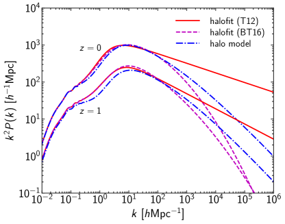
Figure 5: Comparison of matter power spectra $P(k)$ without the baryonic effects computed from the halo model presented in this paper (dash-dotted) with the halofit models of Takahashi et al. (2012, T12) (solid) and Ben-Dayan & Takahashi (2016, BT16) (dashed). The comparisons are made at redshift $z=0$ (upper) and $z=1$ (lower).

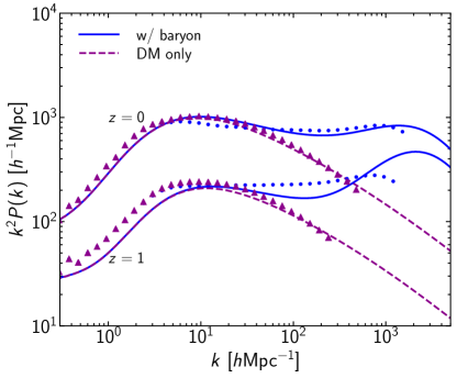
Figure 6: Comparison of matter power spectra $P(k)$ computed from the halo model presented in this paper with IllustrisTNG cosmological hydrodynamical simulations (Nelson et al., 2018; Springel et al., 2018; Pillepich et al., 2018; Marinacci et al., 2018; Naiman et al., 2018). Filled circles and filled triangles show matter power spectra measured in TNG100-1 and TNG100-1-Dark, respectively, whereas solid and dashed lines show halo model predictions with and without baryonic effects, respectively. The comparisons are made at redshift $z=0$ (upper) and $z=1$ (lower).

2.5 Comparisons with Other Results

We compare our halo model calculations with other results of the matter power spectrum to check their validity. One of the most popular models of the matter power spectrum without baryonic effects is the so-called the halofit model, which is originally proposed by Smith et al. (2003) and later improved by Takahashi et al. (2012). The halofit model is essentially a fitting formula whose functional form is motivated by the halo model. In Takahashi et al. (2012), model parameters are calibrated by $N$-body simulation results at $k<30h{\rm Mpc}^{-1}$. Ben-Dayan & Takahashi (2016) updated the halofit model at high wavenumber further by recalibrating model parameters with $N$-body simulation results at $k<300h{\rm Mpc}^{-1}$. In Figure 5, we compare our halo model calculations without baryonic effects with the halofit models of both Takahashi et al. (2012) and Ben-Dayan & Takahashi (2016). We find that at $k<30h{\rm Mpc}^{-1}$ and $k<300h{\rm Mpc}^{-1}$ our halo model results agree well with the halofit models of Takahashi et al. (2012) and Ben-Dayan & Takahashi (2016), respectively. At higher wavenumber $k$, however, disagreements between different models get quite large. Since our halo model is built on well-known properties of halos, we believe our halo model predicts the matter power spectrum at high $k$ much more accurately than the halofit models for which calculations of matter power spectra at high $k$ have to rely on extrapolations of the fitting formulae.

To check the validity of our halo model including the baryonic stellar components, we need to compare our results with matter power spectra measured in cosmological hydrodynamical simulations. For this purpose, we measure matter power spectra from IllustrisTNG cosmological hydrodynamical simulations (Nelson et al., 2018; Springel et al., 2018; Pillepich et al., 2018; Marinacci et al., 2018; Naiman et al., 2018). Specifically, we measure matter power spectra for both TNG100-1 (with baryonic effects) and TNG100-1-Dark (without baryonic effects) that are publicly available and have the box size of $(110.7\leavevmode\nobreak\ {\rm Mpc})^{3}$. Figure 6 compares $P(k)$ from the halo model and IllustrisTNG cosmological hydrodynamical simulations. We find that halo model predictions agree reasonably well with matter power spectra from IllustrisTNG up to $k\sim 10^{3}h{\rm Mpc}^{-1}$. We thus conclude that our halo model is suited form studying the behavior of the matter power spectrum at very high $k$.

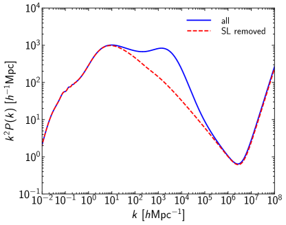
Figure 7: Effects of removing central regions of halos that can produce strong lensing. The solid line shows the original halo model matter power spectrum at $z=0$, whereas the dashed line shows the result after removing those central regions following Equation (23).

2.6 Contribution of Strong Lensing

Figure 3 suggests that the matter power spectrum at $k\sim 10^{3}h{\rm Mpc}^{-1}$ is dominated by the stellar mass components of halos with $M\sim 10^{13}h^{-1}M_{\odot}$ or so. The central region of such halos is known to be a typical site for strong gravitational lensing. Thus gravitational lensing dispersions caused by such component must be highly non-Gaussian i.e., only a tiny fraction of strong lensing events dominate the signal, which complicates the analysis in observations. For instance, that highly non-Gaussian component does not contribute to the gravitational lensing dispersion once strongly lensed events, which can be identified in observations relatively easily, are removed from the sample to derive the dispersion (e.g., Hada & Futamase, 2016, 2019).

We evaluate the significance of such highly non-Gaussian contributions corresponding to strong lensing as follows. We compute the matter power spectrum including a suppression of centers of halos within Einstein radii of a typical strong lensing configuration. Specifically, we modify the Fourier transform of the halo density profile as

$$u(k)\rightarrow u(k)\exp\left(-k^{2}R_{\rm Ein,fid}^{2}\right),$$ (23)

where $u$ refers to both $u_{\rm h}$ and $u_{\rm sub}$, $R_{\rm Ein,fid}$ indicates the comoving Einstein radius of a singular isothermal sphere with a fixed lens redshift $z=0.5$ and source redshift $z_{s}=\infty$

$$R_{\rm Ein,fid}=4\pi\left(\frac{\sigma_{v}}{c}\right)^{2}\chi(z=0.5),$$ (24)

with $\sigma_{v}$ being the velocity dispersion that is estimated from the stellar mass $M_{*}$ (i.e., $f_{*}M$ for halos and $f^{\rm s}_{*}m$ for subhalos) using the observed scaling relation $\log(\sigma_{v}[{\rm km\,s^{-1}}])=-1.4+0.33\log(M_{*}[M_{\odot}])$ (Quimby et al., 2014). In this model, the Einstein radius reduces to zero when halos contain no star, which is reasonable approximation because the NFW profile alone has a negligibly small Einstein radius in the low-mass limit (see e.g., Oguri, 2019).

We show the result in Figure 7. As expected, the matter power spectrum at $10^{2}h{\rm Mpc}^{-1}\lesssim k\lesssim 10^{5}h{\rm Mpc}^{-1}$ is significantly affected by removing strong lensing regions of halos. In contrast, the matter power spectrum $k\sim 10^{6}h{\rm Mpc}^{-1}$ is mostly unaffected, indicating that contributions from such highly non-Gaussian strong lensing regions are not dominant.

Since the contribution of strong lensing is not drastic in the wavenumber range of our interest, in what follows we compute $P(k)$ without removing strong lensing regions unless otherwise stated. We give additional discussions on effects of strong lensing in Section 4.2.

2.7 Effects of Primordial Black Holes

Primordial Black Holes (PBHs) are black holes generated in the early Universe and are a viable candidate of dark matter (see e.g., Sasaki et al., 2018; Carr et al., 2020, for reviews). Here we investigate effects of PBHs on the small-scale matter power spectrum.

First, as in the case of stars, the shot noise from PBHs affects the power spectrum. Denoting the total mass fraction of PBHs to dark matter as $f_{\rm PBH}=\Omega_{\rm PBH}/\Omega_{\rm DM}$ where $\Omega_{\rm DM}=\Omega_{\rm m}-\Omega_{\rm b}$ and the mass of each PBH as $M_{\rm PBH}$, the comoving number density of PBHs is written as

$$\bar{n}_{\rm PBH} = 7.224\times 10^{10}(h{\rm Mpc}^{-1})^{3}$$ (25)

$$\times f_{\rm PBH}\left(\frac{\Omega_{\rm DM}}{0.26}\right)\left(\frac{M_{\rm PBH}}{1h^{-1}M_{\odot}}\right)^{-1}.$$

The contribution of the shot noise to the matter power spectrum is simply given by

$$\Delta P_{\rm shot}(k)=\frac{f_{\rm PBH}^{2}}{\bar{n}_{\rm PBH}}.$$ (26)

Previous studies suggest that the Poisson fluctuation of the PBH number density can be interpreted as an isocurvature perturbation (e.g., Afshordi et al., 2003; Gong & Kitajima, 2017; Inman & Ali-Haïmoud, 2019). We write the isocurvature power spectrum due to the Poisson fluctuation as

$$\Delta P_{\rm iso}(k)=\left\{D_{+}(z)T_{\rm iso}(k)\right\}^{2}\frac{f_{\rm PBH}^{2}}{\bar{n}_{\rm PBH}},$$ (27)

where the transfer function is approximated by

$$T_{\rm iso}(k)=\begin{cases}\frac{3}{2}(1+z_{\rm eq})&(k_{\rm eq}<k<0.1k_{*}),\\ 0&({\rm otherwise}),\end{cases}$$ (28)

where $z_{\rm eq}$ is the redshift at the matter-radiation equality and $k_{\rm eq}=c^{-1}H(z_{\rm eq})(1+z_{\rm eq})^{-1}$ is the inverse of the comoving Hubble horizon size at $z=z_{\rm eq}$. We truncate the transfer function at $k\gtrsim k_{*}$, where $k_{*}=(2\pi^{2}\bar{n}_{\rm PBH})^{1/3}$ is the inverse of the length scale within which there is on average one PBH and is given by

$$k_{*} = 1.126\times 10^{4}h{\rm Mpc}^{-1}$$ (29)

$$\times f_{\rm PBH}^{1/3}\left(\frac{\Omega_{\rm DM}}{0.26}\right)^{1/3}\left(\frac{M_{\rm PBH}}{1h^{-1}M_{\odot}}\right)^{-1/3},$$

because the discreteness effects of PBHs become important as such small scales. For instance, the fluid approximation used for the calculation of the evolution of the isocurvature density fluctuations clearly breaks down at $k\gtrsim k_{*}$. In addition, halos containing the small ($\lesssim 10^{3}$) number of PBHs may be evaporated due to the relaxation (Afshordi et al., 2003). We approximately take account of these effects by truncating the transfer function at $k>0.1k_{*}$.

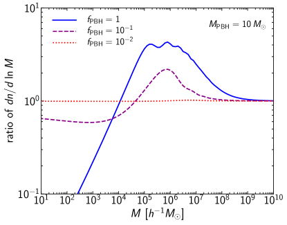
Figure 8: The enhancement of the halo mass function $dn/d\ln M$ due to PBHs i.e., the ratio of $dn/d\ln M$ with PBHs to $dn/d\ln M$ without PBHs. The mass of PBHs is fixed to $M_{\rm PBH}=10\leavevmode\nobreak\ M_{\odot}$, whereas the total mass fractions are $f_{\rm PBH}=1$ (solid), $10^{-1}$ (dashed), and $10^{-2}$ (dotted).

We include the effects of PBHs in our calculation of the nonlinear matter power spectrum as follows. First, we add the contribution of the isocurvature perturbation (equation 27) to the standard adiabatic linear matter power spectrum to compute the square root of the mass variance $\sigma(M)$. By doing so the effect of PBHs is included in the mass functions of main halos and subhalos, as well as the concentration parameter of main halos. We show examples of modifications of the halo mass function due to the isocurvature perturbation in Figure 8. After computing the nonlinear matter power spectrum using the halo model, we add the shot noise contribution (equation 26) to the nonlinear matter power spectrum.

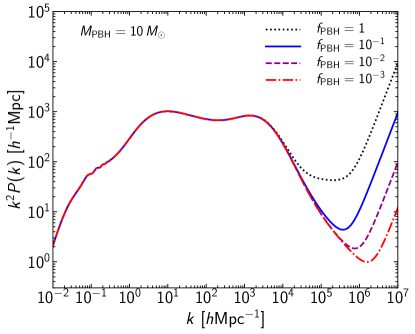
Figure 9: Effects of PBHs on the matter power spectrum $P(k)$ at $z=0$ assuming $M_{\rm PBH}=10\leavevmode\nobreak\ M_{\odot}$. The total mass fractions are $f_{\rm PBH}=1$ (dotted), $10^{-1}$ (solid), $10^{-2}$ (dashed), and $10^{-3}$ (dash-dotted).

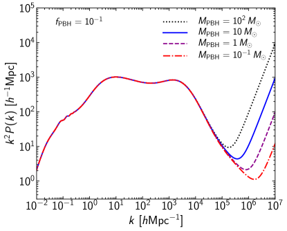
Figure 10: Similar to Figure 9, but the total mass fraction is fixed to $f_{\rm PBH}=10^{-1}$ and masses of PBHs of $M_{\rm PBH}=10^{2}\leavevmode\nobreak\ M_{\odot}$ (dotted), $M_{\rm PBH}=10\leavevmode\nobreak\ M_{\odot}$ (solid), $M_{\rm PBH}=1\leavevmode\nobreak\ M_{\odot}$ (dashed), and $M_{\rm PBH}=10^{-1}\leavevmode\nobreak\ M_{\odot}$ (dash-dotted) are considered.

We show several examples in Figures 9 and 10. We find that PBHs can significantly enhance the small scale matter power spectrum at $k\gtrsim 10^{5}h{\rm Mpc}^{-1}$ due to the enhanced number of dark low-mass halos as well as the shot noise from PBHs. Thus observations of small scale matter power spectra not only directly probe dark low-mass halos but also can constrain the mass and abundance of PBHs.

3 Gravitational Lensing Dispersions

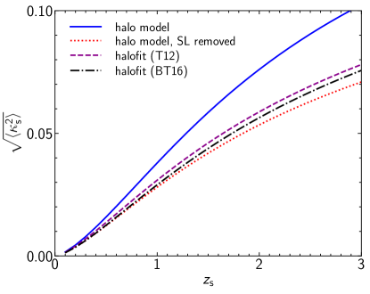
Figure 11: Gravitational lensing dispersions (equation 30) as a function of the source redshift $z_{\rm s}$ for the geometric optics case, assuming a compact source size of $\beta_{\rm s}=10^{-3}$ arcsec. We show results using our halo model including effects of baryon and subhalos (solid), our halo model but the contribution of strong lensing is removed following the prescription in Section 2.6 (dotted), the halofit model of Takahashi et al. (2012, T12) (dashed), and the halofit model of Ben-Dayan & Takahashi (2016, BT16) (dash-dotted).

3.1 Geometric Optics Case

Geometric optics provides a good approximation for calculating gravitational lensing dispersions of traditional astronomical sources such as supernovae. In this case the dispersion of convergence smoothed over the angular size $\beta_{\rm s}$ is given by (e.g., Takahashi et al., 2011)

$$\langle\kappa_{\rm s}^{2}\rangle=\int_{0}^{\chi_{\rm s}}d\chi\,W^{2}(\chi)\int\frac{k\,dk}{2\pi}P(k)W_{\rm s}^{2}(k\chi\beta_{\rm s}),$$ (30)

where $\chi$ is the radial distance, $\chi_{\rm s}$ is the radial distance to the source, the $W(\chi)$ is a lensing weight function given by (note that $\bar{\rho}$ here is the comoving matter density)

$$W(\chi)=\frac{4\pi G}{c^{2}}\bar{\rho}a^{-1}\frac{\chi(\chi_{\rm s}-\chi)}{\chi_{\rm s}},$$ (31)

and $W_{\rm s}(x)$ is a smoothing kernel for which we assume a top-hat filter

$$W_{\rm s}(x)=\frac{2J_{1}(x)}{x}.$$ (32)

In most cases, the dispersion of magnification rather than that of convergence is observed. For a similarly smoothed magnification $\mu_{\rm s}$, a weak lensing approximation

$$\mu_{\rm s}\approx 1+2\kappa_{\rm s},$$ (33)

is expected to hold when $|\mu_{\rm s}-1|\ll 1$, and in this case we simply have $\langle(\mu_{\rm s}-1)^{2}\rangle\approx 4\langle\kappa_{\rm s}^{2}\rangle$.

Figure 11 shows examples of dispersions of convergence computed using our halo model as well as the halofit model. We find that our halo model including baryonic effects predicts significantly larger dispersions than halofit model predictions for which baryonic effects are not included. However, as discussed in Section 2.6, the significant fraction of the enhancement by baryonic effects comes from centers of massive galaxies that produce strong lensing. Once such regions are removed from the calculation of the matter power spectrum (see Section 2.6 for more details), we find that gravitational lensing dispersions from our halo model with baryonic effects approximately match those from the halofit model for which baryonic effects are not included.

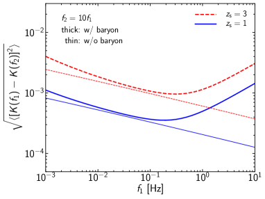
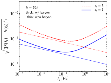
Figure 12: Left: Gravitational lensing dispersion of the gravitational wave amplitude (equation 40) for $z_{\rm s}=1$ (solid) and $z_{\rm s}=3$ (dashed) as a function of $f_{1}$. The frequency $f_{2}$ is fixed to $f_{2}=10f_{1}$. Thick and thin lines show calculations with and without baryonic effects, respectively. Right: Similar to the left panel, but for gravitational lensing dispersion of the gravitational wave phase (equation 42).

3.2 Wave Optics Case

The propagation of gravitational waves in the inhomogeneous density field has been studied in the literature, which indicates that density fluctuations below the Fresnel scale $\sim(f\chi_{\rm s})^{1/2}$ (Macquart, 2004; Takahashi et al., 2005; Takahashi, 2006) are subject to the wave effect and does not affect the propagation of gravitational waves due to diffraction effects. We provide detailed calculations in Appendix C, and here we give a short summary. We denote $\phi^{0}_{\rm obs}(f)$ as observed gravitational waves at frequency $f$ in absence of gravitational lensing and $\phi_{\rm obs}(f)$ as observed gravitational waves with gravitational lensing effects. Adopting the weak lensing approximation, gravitational lensing effects can be described by small amplitude and phase shifts $K(f)$ and $S(f)$

$$\frac{\phi_{\rm obs}(f)}{\phi^{0}_{\rm obs}(f)}\approx\left[1+K(f)\right]e^{iS(f)}.$$ (34)

In the geometric optics limit $K(f)$ and $S(f)$ reduce to convergence and gravitational time delay, respectively. Dispersions of $K(f)$ and $S(f)$ are computed as

$$\langle K^{2}(f)\rangle=\int_{0}^{\chi_{\rm s}}d\chi W^{2}(\chi)\int\frac{k\,dk}{2\pi}P(k)F_{K}^{2},$$ (35)

$$F_{K}=\frac{\sin(r_{\rm F}^{2}k^{2}/2)}{r_{\rm F}^{2}k^{2}/2},$$ (36)

$$\langle S^{2}(f)\rangle=\int_{0}^{\chi_{\rm s}}d\chi W^{2}(\chi)\int\frac{k\,dk}{2\pi}P(k)F_{S}^{2},$$ (37)

$$F_{S}=\frac{\cos(r_{\rm F}^{2}k^{2}/2)-1}{r_{\rm F}^{2}k^{2}/2},$$ (38)

where $r_{\rm F}$ denotes the Fresnel scale (Macquart, 2004; Takahashi et al., 2005; Takahashi, 2006)

$$r_{\rm F}=\sqrt{\frac{c\chi(\chi_{\rm s}-\chi)}{2\pi f\chi_{\rm s}}}.$$ (39)

Equation (35) suggests that the Fresnel scale can be interpreted as an effective source size, as is also discussed in Appendix D.

As discussed in Appendix C, $K(f)$ and $S(f)$ can be measured by comparing inspiral waveforms at different frequencies

$$\left\langle\left[K(f_{1})-K(f_{2})\right]^{2}\right\rangle=\int_{0}^{\chi_{\rm s}}d\chi W^{2}(\chi)\int\frac{k\,dk}{2\pi}P(k)F_{K,12}^{2},$$ (40)

$$F_{K,12}=\frac{\sin(r_{\rm F1}^{2}k^{2}/2)}{r_{\rm F1}^{2}k^{2}/2}-\frac{\sin(r_{\rm F2}^{2}k^{2}/2)}{r_{\rm F2}^{2}k^{2}/2},$$ (41)

$$\left\langle\left[S(f_{1})-S(f_{2})\right]^{2}\right\rangle=\int_{0}^{\chi_{\rm s}}d\chi W^{2}(\chi)\int\frac{k\,dk}{2\pi}P(k)F_{S,12}^{2},$$ (42)

$$F_{S,12}=\frac{\cos(r_{\rm F1}^{2}k^{2}/2)-1}{r_{\rm F1}^{2}k^{2}/2}-\frac{\cos(r_{\rm F2}^{2}k^{2}/2)-1}{r_{\rm F2}^{2}k^{2}/2},$$ (43)

where $r_{\rm F1}$ and $r_{\rm F2}$ denote the Fresnel scales (equation 39) evaluated at frequency $f_{1}$ and $f_{2}$, respectively. We can also consider the cross-correlation between $K(f)$ and $S(f)$ as

$$\left\langle\left[K(f_{1})-K(f_{2})\right]\left[S(f_{1})-S(f_{2})\right]\right\rangle$$ (44)

$$=\int_{0}^{\chi_{\rm s}}d\chi W^{2}(\chi)\int\frac{k\,dk}{2\pi}P(k)F_{K,12}F_{S,12}.$$

We show some examples in Figures 12. Since the Fresnel scale is proportional to $f^{-1/2}$ (see equation 39), at lower frequency the dispersion probe the matter power spectrum at smaller $k$. Effects of baryon are minimized around the frequency of $f\sim 0.1$ Hz, where the matter power spectrum at $k\sim 10^{6}h{\rm Mpc}^{-1}$ is probed. At frequency higher than $f\sim 0.1$ Hz, the dispersion quickly increases because of the shot noise from stars. Gravitational wave observations around $f\sim 0.1$ Hz will be conducted by e.g., B-DECIGO (Nakamura et al., 2016). However, expected dispersions are small, $\mathcal{O}(10^{-3})$, suggesting that high $S/N$ observations for many events are needed to detect the dispersions. Some discussions on the detectability are given in Section 4.1.

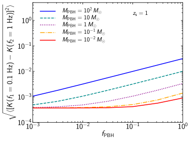
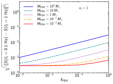
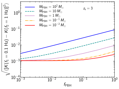
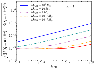
Figure 13: Gravitational lensing dispersions of gravitational wave amplitude (equation 40) and phase (equation 42) are shown in left and right panels, respectively. Upper panels show results at $z_{\rm s}=1$ and lower panels show results at $z_{\rm s}=3$. Frequencies are fixed to $f_{1}=0.1\leavevmode\nobreak\ {\rm Hz}$ and $f_{2}=1\leavevmode\nobreak\ {\rm Hz}$. In each panel, gravitational lensing dispersions as a function of PBH fraction $f_{\rm PBH}$ for several different PBH masses are shown.

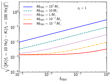
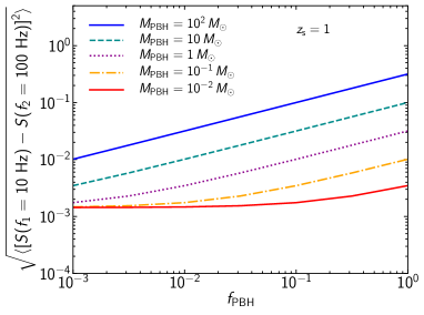
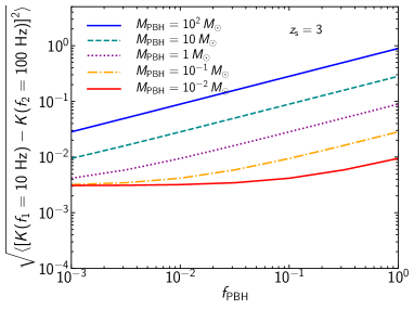
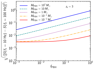
Figure 14: Similar to Figure 13, but for frequencies $f_{1}=10\leavevmode\nobreak\ {\rm Hz}$ and $f_{2}=100\leavevmode\nobreak\ {\rm Hz}$.

3.3 Enhancement due to Primordial Black Holes

As shown in Section 2.7, the presence of PBHs can significantly enhance the matter power spectrum at high $k$, suggesting that observations of gravitational lensing dispersions of gravitational waves can be used to constrain the abundance of PBHs. We explore this possibility using our model of the matter power spectrum presented in Section 2.7.

We show results in Figures 13 and 14. Here we consider two combinations of frequency ranges, from $f_{1}=0.1\leavevmode\nobreak\ {\rm Hz}$ and $f_{2}=1\leavevmode\nobreak\ {\rm Hz}$ corresponding to space observations of gravitational waves (Figure 13), and from $f_{1}=10\leavevmode\nobreak\ {\rm Hz}$ and $f_{2}=100\leavevmode\nobreak\ {\rm Hz}$ corresponding to ground observations of gravitational waves (Figure 14). We find that the enhancement of gravitational lensing dispersion by PBHs is indeed significant, more than an order of magnitude in some cases. The enhancement is particularly large for $f_{1}=10\leavevmode\nobreak\ {\rm Hz}$ and $f_{2}=100\leavevmode\nobreak\ {\rm Hz}$, for which the shot noise from PBHs dominates gravitational lensing dispersion (see also Section 2.7). Weak lensing by the shot noise is discussed further in Section 4 and Appendix D. Since the shot noise power spectrum (equation 26) is $\Delta P_{\rm shot}(k)=f_{\rm PBH}^{2}/\bar{n}_{\rm PBH}\propto f_{\rm PBH}M_{\rm PBH}$ for a fixed $\Omega_{\rm DM}$, gravitational lensing dispersions at the shot noise dominated region behave as $\propto\sqrt{f_{\rm PBH}M_{\rm PBH}}$ as shown in Figure 14.

4 Discussions

4.1 Detectability

For each gravitational wave event, we can measure amplitude and phase fluctuations with an accuracy of $\sim 1/\rho$, where $\rho$ denotes the signal-to-noise ratio of the gravitational wave observation (Lindblom et al., 2008). Unless gravitational lensing dispersions are significantly boosted by PBHs, its typical value is $\mathcal{O}(10^{-3})$, indicating that $\rho\gtrsim 10^{3}$ is needed to directly measure amplitude and phase shifts due to gravitational lensing for individual gravitational wave events. We use the calculation method described in Oguri (2018) to estimate $\rho$ for the chirp mass of $30\leavevmode\nobreak\ M_{\odot}$ and the redshift of $1$ and find that $\rho\sim 30$ for B-DECIGO and $\rho\sim 60$ for Einstein Telescope. Therefore measurements of gravitational lensing dispersions are likely to be achieved by combining observations of many gravitational wave events. For instance, by combining $N_{\rm event}$ gravitational wave events, we can measure amplitude and phase dispersions down to $\sim(2/N_{\rm event})^{1/4}(1/\rho)$, suggesting that $N_{\rm event}=3\times 10^{5}$ with $\rho=50$ leads to the measurement of the dispersion at the level of $10^{-3}$. The required number is large but can be achieved by next-generation gravitational wave experiments. Alternatively, observations of the modest number of events with very sensitive space based gravitational wave detectors such as DECIGO (Seto et al., 2001) may allow us to measure gravitational lensing dispersions.

We note that measurements of gravitational lensing dispersions do not necessarily require measurements of redshifts of individual gravitational wave events. For instance, by considering the ratio of strain amplitudes at different frequencies the dependence on the distance to the gravitational wave source cancels out. The dependence on antenna pattern functions also cancels out if the frequency evolution is much faster than the change of antenna pattern functions with time. The dispersion of phases may also be measured without knowing the distance to the source, although the degeneracy with binary model parameters may be in issue. We leave detailed studies of measurements of gravitational lensing dispersions in a realistic setup for future work.

4.2 Validity of Weak Lensing Approximation

Since our results rely on the weak lensing approximation, it is important to check the validity of the approximation. This is partly done in Section 2.6 in which the matter power spectrum at $k\sim 10^{6}h{\rm Mpc}^{-1}$, which is responsible for gravitational lensing dispersions at $f\sim 0.1-1$ Hz, is shown to be largely unaffected by removing central regions of galaxies that can produce strong lensing. This is because the matter power spectrum at $k\sim 10^{6}h{\rm Mpc}^{-1}$ mostly originates from halos and subhalos with masses $1h^{-1}M_{\odot}\lesssim M\lesssim 10^{4}h^{-1}M_{\odot}$. Such low-mass halos do not contain stars, and the convergence $\kappa$ of such halos computed from the NFW (or BMO) profile is quite low because it is proportional to $\rho_{\rm s}r_{\rm s}\propto r_{\rm vir}c^{2}/f_{\rm NFW}(c)$. Given the weak dependence of $c$ on the halo mass, $\kappa$ is a increasing function of the mass such that $\kappa\ll 1$ even at the very central region for halos and subhalos with masses $1h^{-1}M_{\odot}\lesssim M\lesssim 10^{4}h^{-1}M_{\odot}$. Thus we can safely adopt the weak lensing approximation for lensing by dark low-mass halos.

When the shot noise contribution to the matter power spectrum is dominant, it is important to make sure that gravitational lensing by individual stars or PBHs is not strong. This condition is written as (see also equation D9)

$$w=\left(\frac{R_{\rm Ein}}{r_{\rm F}}\right)^{2}=2\pi f(1+z)\frac{4Gm_{\rm p}}{c^{3}}<1,$$ (45)

where $R_{\rm Ein}$ is the Einstein radius (equation D4) and $m_{\rm p}$ refers to either individual mass of stars $m_{\rm star}$ or individual mass of PBHs $M_{\rm PBH}$. This condition translates into $m_{\rm p}<81(1+z)^{-1}(f/100\leavevmode\nobreak\ {\rm Hz})^{-1}M_{\odot}$, where $f=100\leavevmode\nobreak\ {\rm Hz}$ is the highest frequency considered in this paper. Therefore, the weak lensing approximation is reasonable for all the situations consider in the paper, except for the case with the PBH mass $M_{\rm PBH}=100\leavevmode\nobreak\ M_{\odot}$ and the frequency range $f=10-100$ Hz for which the weak lensing approximation is partly broken and thus the result should be taken with caution.

4.3 Degree of Non-Gaussianity

Another question to ask is how well the distributions of $K$ and $S$ are described by Gaussian. For instance, if the signal is dominated by a tiny fraction of strong lensing events the resulting distribution is quite non-Gaussian as partly discussed in Section 2.6. While this can be studied by computing higher-order statistics such as skewness and kurtosis, here we make a simple evaluation of the degree of non-Gaussianity based on the average number of lenses that contribute to the dispersion. Discussions in Appendix D indicate that lenses that fall within the Fresnel scale contribute to the dispersion when the weak lensing approximation is valid. When the average number of lenses is much large than unity, the central limit theorem assures that the distribution is close to the Gaussian distribution, whereas the average number is small, say less than unity, we expect the distribution with a significant skewness.

The average number $\bar{N}_{\rm proj}$ of any lenses with the comoving number density $\bar{n}$, which is assumed to be independent of redshift for simplicity, within the Fresnel scale integrated along the line-of-sight is given by

$$\bar{N}_{\rm proj}=\int_{0}^{\chi_{\rm s}}d\chi\,4r_{\rm F}^{2}\bar{n}=V_{\rm F}\bar{n},$$ (46)

where the origin of the prefactor 4 in the right hand size is discussed in Appendix D. We find $V_{\rm F}\approx 3.70\times 10^{-9}(f/1\leavevmode\nobreak\ {\rm Hz})^{-1}(h^{-1}{\rm Mpc})^{3}$ for $z_{\rm s}=1$ and $V_{\rm F}\approx 1.36\times 10^{-8}(f/1\leavevmode\nobreak\ {\rm Hz})^{-1}(h^{-1}{\rm Mpc})^{3}$ for $z_{\rm s}=3$. On the other hand, the number density of dark low-mass halos with $1h^{-1}M_{\odot}\lesssim M\lesssim 10^{4}h^{-1}M_{\odot}$ is $\sim 10^{8}(h^{-1}{\rm Mpc})^{-3}$. Thus we expect a moderately skewed distribution for gravitational lensing dispersions at $f\sim 0.1-1$ Hz by dark low-mass halos at least when $z_{\rm s}\lesssim 3$. Since the volume $V_{\rm F}$ increases with increasing source redshift $z_{\rm s}$, the distribution should approach to the Gaussian distribution for very high source redshift $z_{\rm s}$.

In the case of gravitational lensing dispersions produced by the shot noise, we can use e.g., equation (25) to estimate the average number $\bar{N}_{\rm proj}$, e.g.,

$$\bar{N}_{\rm proj}\approx 270\left(\frac{f}{1\leavevmode\nobreak\ {\rm Hz}}\right)^{-1}f_{\rm PBH}\left(\frac{M_{\rm PBH}}{1h^{-1}M_{\odot}}\right)^{-1},$$ (47)

for $z_{\rm s}=1$, and

$$\bar{N}_{\rm proj}\approx 980\left(\frac{f}{1\leavevmode\nobreak\ {\rm Hz}}\right)^{-1}f_{\rm PBH}\left(\frac{M_{\rm PBH}}{1h^{-1}M_{\odot}}\right)^{-1},$$ (48)

for $z_{\rm s}=3$. Thus in the range of parameters we examine in this paper there are both cases with $\bar{N}_{\rm proj}>1$ and $\bar{N}_{\rm proj}<1$. We note that when $\bar{N}_{\rm proj}\ll 1$ the situation is close to the one considered by Zumalacárregui & Seljak (2018) in which the non-Gaussian magnification probability distribution function due to gravitational lensing by single PBH masses is used to constrain the abundance of PBHs.

For both dark low-mass halos and PBHs, there are cases when single events dominate the signal depending on frequencies of gravitational waves and the mass of lenses. In such cases, it may be possible to detect individual weak lensing events directly by making use of the wavelength dependence of the signal. For instance, the amplitude is affected by weak lensing as Equations (D9) and (D11), which indicates that weak lensing may be detected via the modulation of the amplitude as a function of frequency that is proportional to $w\propto f$ (for PBH) if the signal-to-noise ratio of the gravitational wave observation is sufficiently high (see also Section 4.1). This possibility is partly studied in Dai et al. (2018a) assuming a singular isothermal sphere as a lens and is worth exploring more in various setups.

5 Conclusion

In this paper we have explored the possibility of using gravitational lensing dispersions of gravitational waves to probe the matter power spectrum at very high $k$ i.e., very small scales. For this purpose we have analyzed the small scale behavior of the matter power spectrum using the halo model, including effects of baryon and subhalos. We have confirmed that our halo model predictions agree reasonably well with results of IllustrisTNG cosmological hydrodynamical simulations. Using this halo model that is built on well-studied halo properties and the stellar mass–halo mass relation, we study the matter power spectrum at $k>10^{3}h{\rm Mpc}^{-1}$ that has been poorly explored before. We find that the matter power spectrum at $k\sim 10^{6}h{\rm Mpc}^{-1}$ is relatively insensitive to baryon effects and is dominated by dark low-mass halos with $1h^{-1}M_{\odot}\lesssim M\lesssim 10^{4}h^{-1}M_{\odot}$. We have also found that the matter power spectrum at $k\gtrsim 10^{5}h{\rm Mpc}^{-1}$ can be significantly enhanced by PBHs due to the enhanced halo formation as well as the shot noise from PBHs.

Using the halo model power spectrum we have computed frequency dependent gravitational lensing dispersions of gravitational waves. The frequency dependence originates from the wave optics nature of the propagation of gravitational waves. We have found that lensing dispersions of the amplitude and phase of gravitational waves are $\mathcal{O}(10^{-3})$ in the frequency range of $f\sim 10^{-3}-100$ Hz for source redshifts of $z_{\rm s}\sim 1-3$. In particular, the frequency range of $f\sim 0.1-1$ Hz is found to be a window appropriate for detecting dark low-mass halos with $1h^{-1}M_{\odot}\lesssim M\lesssim 10^{4}h^{-1}M_{\odot}$. PBHs with $M\gtrsim 0.1\leavevmode\nobreak\ M_{\odot}$ can enhance gravitational lensing dispersions more than an order of magnitude, when they constitute a significant fraction of dark matter. At the frequency range of $f\sim 10-100$ Hz, which corresponds to frequencies of ground observations of gravitational waves, gravitational lensing dispersions are dominated by the shot noise from PBHs and therefore serve as a useful probe of PBHs.

Appendix A Halo Model Calculations

Here we summarize the derivations of the halo model power spectrum both in the standard case (Section 2.1) and with modifications including stellar components and subhalos (Section 2.2).

First, we derive the standard halo model power spectrum. We start with Equation (1) and rewrite it as

$$\rho(\boldsymbol{x})=\sum_{i}\int dM\int d\boldsymbol{x}^{\prime}\delta^{\rm D}(M-M_{i})\delta^{\rm D}(\boldsymbol{x}^{\prime}-\boldsymbol{x}_{i})\,M\,u\left(\boldsymbol{x}-\boldsymbol{x}^{\prime}|M\right),$$ (A1)

where $\delta^{\rm D}$ denotes the Dirac delta function. The halo mass function $dn/dM$ is given by

$$\frac{dn}{dM}=\left\langle\sum_{i}\delta^{\rm D}(M-M_{i})\delta^{\rm D}(\boldsymbol{x}^{\prime}-\boldsymbol{x}_{i})\right\rangle,$$ (A2)

from which it is shown that

$$\left\langle\rho(\boldsymbol{x})\right\rangle=\int dM\,M\frac{dn}{dM}=\bar{\rho},$$ (A3)

where $\bar{\rho}$ is the mean comoving density of the Universe. We now consider density fluctuations. Their expressions in real and Fourier spaces are given as

$$\delta(\boldsymbol{x})=\frac{\rho(\boldsymbol{x})}{\bar{\rho}}-1,$$ (A4)

$$\delta(\boldsymbol{k})=\int d\boldsymbol{x}\,\delta(\boldsymbol{x})\,e^{-i\boldsymbol{k}\cdot\boldsymbol{x}}.$$ (A5)

From Equation (A1), $\delta(\boldsymbol{k})$ is calculated as

$$\delta(\boldsymbol{k})=\frac{1}{\bar{\rho}}\sum_{i}\int dM\int d\boldsymbol{x}\,\delta^{\rm D}(M-M_{i})\delta^{\rm D}(\boldsymbol{x}-\boldsymbol{x}_{i})\,M\,u\left(\boldsymbol{k}|M\right)\,e^{-i\boldsymbol{k}\cdot\boldsymbol{x}},$$ (A6)

where $u\left(\boldsymbol{k}|M\right)=u\left(k|M\right)$ assuming a statistically spherical symmetric halo shape is the Fourier transform of the normalized density profile $u(\boldsymbol{x}|m)$. From this expression, we compute the correlation of $\delta(\boldsymbol{k})$

$$\langle\delta(\boldsymbol{k})\delta(\boldsymbol{k}^{\prime})\rangle=V\delta^{\rm D}(\boldsymbol{k}+\boldsymbol{k}^{\prime})P(k),$$ (A7)

from which the power spectrum is computed as

$$P(k) = P^{\rm 1h}(k)+P^{\rm 2h}(k)$$ (A8)

$$= \int dM\frac{dn}{dM}\left(\frac{M}{\bar{\rho}}\right)^{2}u^{2}(k|M)+\int dM_{1}\frac{dn}{dM_{1}}\left(\frac{M_{1}}{\bar{\rho}}\right)u(k|M_{1})\int dM_{2}\frac{dn}{dM_{2}}\left(\frac{M_{2}}{\bar{\rho}}\right)u(k|M_{2})\,P_{\rm hh}(k|M_{1},M_{2}),$$

where

$$\left\langle\sum_{i,j}\delta^{\rm D}(M-M_{i})(M^{\prime}-M_{j})\delta^{\rm D}(\boldsymbol{x}-\boldsymbol{x}_{i})\delta^{\rm D}(\boldsymbol{x}^{\prime}-\boldsymbol{x}_{j})\right\rangle=\frac{dn}{dm_{1}}\frac{dn}{dm_{2}}\xi_{\rm hh}(|\boldsymbol{x}-\boldsymbol{x}^{\prime}||M_{1},M_{2}),$$ (A9)

$\xi_{\rm hh}$ is the halo-halo correlation function, and $P_{\rm hh}$ is its Fourier counterpart. In what follows we simply assume a linear halo bias

$$P_{\rm hh}(k|M_{1},M_{2})=b(M_{1})b(M_{2})P_{\rm lin}(k),$$ (A10)

where $P_{\rm lin}(k)$ is the linear matter power spectrum. In this case the 2-halo term reduces to Equation (4).

Next we consider modifications of 1-halo term. Starting from Equation (5), the Fourier transform of the density fluctuation is written as

$$\delta(\boldsymbol{k}) = \frac{1}{\bar{\rho}}\sum_{i}\int dM\int d\boldsymbol{x}\,\delta^{\rm D}(M-M_{i})\delta^{\rm D}(\boldsymbol{x}-\boldsymbol{x}_{i})(1-f_{\rm s})M\,u_{\rm h}\left(\boldsymbol{k}|M\right)\,e^{-i\boldsymbol{k}\cdot\boldsymbol{x}}$$ (A11)

$$+\frac{1}{\bar{\rho}}\sum_{i,j}\int dM\int dm\int d\boldsymbol{x}\int d\boldsymbol{x}^{\prime}\delta^{\rm D}(M-M_{i})\delta^{\rm D}(m-m_{j})\delta^{\rm D}(\boldsymbol{x}-\boldsymbol{x}_{i})\delta^{\rm D}(\boldsymbol{x}^{\prime}-\boldsymbol{x}_{j})m\,u_{\rm sub}\left(\boldsymbol{k}|M,m\right)\,e^{-i\boldsymbol{k}\cdot\boldsymbol{x}^{\prime}},$$

where we ignored the dependence of $u_{\rm sub}$ on the position within a halo i.e., $u_{\rm sub}(\boldsymbol{x}-\boldsymbol{x}_{j}|M_{i},m_{j},\boldsymbol{x}_{j}-\boldsymbol{x}_{i})=u_{\rm sub}(\boldsymbol{x}-\boldsymbol{x}_{j}|M_{i},m_{j})$. We also need to specify the subhalo mass function $dN_{i}/dm$ and their spatial distribution $U(\boldsymbol{x}-\boldsymbol{x}_{i}|M_{i},m)$ within the $i$-th halo, which is given in a manner similar to Equation (A2) as

$$\frac{dN_{i}}{dm}U(\boldsymbol{x}^{\prime}-\boldsymbol{x}_{i}|M_{i},m)=\left.\left\langle\sum_{j}\delta^{\rm D}(m-m_{j})\delta^{\rm D}(\boldsymbol{x}^{\prime}-\boldsymbol{x}_{j})\right\rangle\right|_{i},$$ (A12)

where they satisfy

$$\int dm\,m\frac{dN_{i}}{dm}=f_{\rm s}M_{i},$$ (A13)

$$\int d\boldsymbol{x}\,U(\boldsymbol{x}-\boldsymbol{x}_{i}|M_{i},m)=1.$$ (A14)

From these relations, it can be easily shown that $\left\langle\rho(\boldsymbol{x})\right\rangle=\bar{\rho}$ also for this modified 1-halo case. From Equations (A7) and (A11), we can derive the 1-halo power spectrum as Equation (8).

As discussed in Section 2.2, the shot noise from stars can become important at very small scales. The effect is evaluated by replacing $u_{*}(\boldsymbol{x}|M)$ as

$$u_{*}(\boldsymbol{x}|M)\rightarrow u_{*}^{\rm s}(\boldsymbol{x}|M)=\frac{1}{N_{*}}\sum_{j}\delta^{\rm D}(\boldsymbol{x}-\boldsymbol{x}_{j}),$$ (A15)

where for simplicity we assume that all stars share the same mass $m_{\rm star}$ and $N_{*}=f_{*}M/m_{\rm star}$ denotes the total number of stars in each halo with mass $M$. The following relation

$$N_{*}u_{*}(\boldsymbol{x}|M)=\left\langle\sum_{j}\delta^{\rm D}(\boldsymbol{x}-\boldsymbol{x}_{j})\right\rangle,$$ (A16)

ensures that $\langle u_{*}^{\rm s}(\boldsymbol{x}|M)\rangle=u_{*}(\boldsymbol{x}|M)$. The Fourier transform of $u_{*}$ is modified as

$$u_{*}(\boldsymbol{k}|M)\rightarrow u_{*}^{\rm s}(\boldsymbol{k}|M)=\frac{1}{N_{*}}\int d\boldsymbol{x}\sum_{j}\delta^{\rm D}(\boldsymbol{x}-\boldsymbol{x}_{j})e^{-i\boldsymbol{k}\cdot\boldsymbol{x}},$$ (A17)

from which we obtain the effect of the shot noise as

$$\left\langle u_{*}^{\rm s}(\boldsymbol{k}|M)u_{*}^{\rm s}(-\boldsymbol{k}|M)\right\rangle=u_{*}(\boldsymbol{k}|M)u_{*}(-\boldsymbol{k}|M)+\frac{1}{N_{*}}.$$ (A18)

That is, we can simply replace $u_{*}^{2}(k|M)$ with $u_{*}^{2}(k|M)+1/N_{*}$ to include the shot noise effect.

Appendix B A Simple Analytic Model of Subhalos

Analytic models of subhalos have been proposed in the literature (e.g., Lee, 2004; Oguri & Lee, 2004; van den Bosch et al., 2005; Giocoli et al., 2008b, a; Han et al., 2016; Jiang & van den Bosch, 2016; Hiroshima et al., 2018; Ando et al., 2019), in which important physical effects such as tidal stripping are taken into account. Here we present a new analytic model of subhalos partly following Oguri & Lee (2004) in which both tidal stripping and dynamical frictions are taken into account. We keep this model as simple as possible so that it can easily be computed numerically.

Following previous work we base our analytic model on the extended Press-Schechter theory (Bond et al., 1991; Bower, 1991; Lacey & Cole, 1993), which predicts the number distribution of progenitors with mass $m_{\rm f}$ at redshift $z_{\rm f}$ for a halo with mass $M$ and redshift $z$ as

$$\frac{dN_{\rm EPS}}{dm_{\rm f}}=\frac{M}{m_{\rm f}}P(m_{\rm f},z_{\rm f}|M,z)dm_{\rm f},$$ (B1)

$$P(m_{\rm f},z_{\rm f}|M,z)=\frac{1}{\sqrt{2\pi}}\frac{\Delta\omega}{\Delta S^{3/2}}\exp\left(-\frac{\Delta\omega^{2}}{2\Delta S}\right)\left|\frac{d\Delta S}{dm_{\rm f}}\right|,$$ (B2)

with $\Delta\omega=\delta_{\rm c}(z_{\rm f})-\delta_{\rm c}(z)$ and $\Delta S=\sigma^{2}(m_{\rm f})-\sigma^{2}(M)$. We adopt $\delta_{\rm c}(z)=(3/20)(12\pi)^{2/3}\left\{\Omega_{\rm m}(z)\right\}^{0.0055}/D_{+}(z)$ (Navarro et al., 1997) with $D_{+}(z)$ being the linear growth rate. The square root of the mass variance $\sigma(M)$ is computed in the standard way by integrating the linear matter power spectrum with a top-hat filter.

We evaluate Equation (B1) at the median formation time of each halo. Following Giocoli et al. (2007), we derive the median formation time by solving the following equation

$$\delta_{\rm c}(z_{\rm f})=\delta_{\rm c}(z)+\frac{0.974}{\sqrt{q}}\sqrt{\sigma^{2}(f_{\rm f}M)-\sigma^{2}(M)},$$ (B3)

where $q=0.707$ and $f_{\rm f}=0.5$.

We consider the effect of mass loss due to tidal stripping. We connect $m_{\rm f}$ and $m$ that refer to subhalo masses before and after tidal stripping as follows

$$m=m_{\rm f}\frac{f_{\rm BMO}(\tau^{\rm ave})}{f_{\rm NFW}\left(c(m_{\rm f},z_{\rm f})\right)},$$ (B4)

$$\tau^{\rm ave}=\frac{r_{\rm t}^{\rm ave}(m,f_{\rm f}M,z_{\rm f})}{r_{s}(m_{\rm f},c,z_{\rm f})},$$ (B5)

$$r_{\rm t}^{\rm ave}(m,M,z)=\int 4\pi r^{2}dr\,r_{\rm t}(r,m,M)U(r|M,m)=\int 4\pi r^{2}dr\,r\left[\frac{m}{3M(<r)}\right]^{1/3}U(r|M,m),$$ (B6)

where $U(r|M,m)$ is the spatial distribution of subhalos and $M(<r)$ is an enclosed mass of the host halo, both of which we compute using the BMO profile.

We also take account of the dynamical friction. We adopt the following crude approximation of the dynamical friction timescale (e.g., Mo et al., 2010)

$$t_{\rm df}(m,M,z)=2\frac{M}{m}\frac{r_{\rm vir}}{V_{\rm vir}(M)},$$ (B7)

where $V_{\rm vir}(M)=\sqrt{GM/r_{\rm vir}}$. The prefactor of 2 is introduced to better reproduce the numerical results. We assume that the subhalo mass function is suppressed by the following factor

$$f_{\rm df}=\exp\left[-\left\{\frac{t(z)-t(z_{\rm f})}{t_{\rm df}(m_{\rm f},f_{\rm f}M,z_{\rm f})}\right\}^{2}\right].$$ (B8)

Finally we combine these results to compute the subhalo mass function as

$$\frac{dn_{M}}{dm}=f_{\rm df}\frac{dN_{\rm EPS}}{dm_{\rm f}}\frac{dm_{\rm f}}{dm}.$$ (B9)

We model the density profile of subhalos by the BMO profile with the truncation radius $r_{\rm t}^{\rm ave}(m,f_{\rm f}M,z_{\rm f})$ by that computed above. For an accurate prediction of the scale radius of each subhalo, we use a fitting form of the concentration parameter for subhalos $c_{\rm sub}$ by Ando et al. (2019, see also ). In order to convert $c_{200}$ to $c_{\rm vir}$ we multiply it by $[200/\Delta_{\rm vir}\Omega_{\rm m}(z)]^{1/3}[H(z)/H_{0}]^{-2/3}$, where $\Delta_{\rm vir}$ is the virial overdensity computed from the spherical collapse model (Nakamura & Suto, 1997). Figure 15 shows examples of subhalo mass functions $dN_{M}/dm$ as well as subhalo mass fractions $f_{\rm s}$.

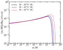
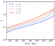
Figure 15: Left: Examples of subhalo mass functions as a function of the subhalo mass $m$ at redshift $z=0$ for three host halo masses $M$. Right: Subhalo mass fractions $f_{\rm s}$ as a function of the host halo mass $M$ at several different redshifts.

Appendix C Weak Gravitational Lensing in Wave Optics

Here we summarize weak gravitational lensing in wave optics, following and extending work by Takahashi et al. (2005) and Takahashi (2006). Under the Born approximation, the observed wave at comoving spatial coordinate $\boldsymbol{x}$ with comoving frequency $f$ in the presence of gravitational potential $\Phi(\boldsymbol{x})$ is

$$\phi(f,\boldsymbol{x})=\phi^{0}(f,\boldsymbol{x})+\delta\phi(f,\boldsymbol{x}),$$ (C1)

$$\delta\phi(f,\boldsymbol{x})=-\frac{4\pi f^{2}}{c^{4}}\int d\boldsymbol{x}^{\prime}\frac{e^{2\pi if|\boldsymbol{x}-\boldsymbol{x}^{\prime}|/c}}{|\boldsymbol{x}-\boldsymbol{x}^{\prime}|}\Phi(\boldsymbol{x}^{\prime})\phi^{0}(f,\boldsymbol{x}^{\prime}),$$ (C2)

where $\phi^{0}(f,\boldsymbol{x})$ denotes the solution with $\Phi(\boldsymbol{x})=0$. Here we adopt a spherical coordinate in a flat Universe, $\boldsymbol{x}$=($\chi$, $\boldsymbol{r}$), centered at the observer with a flat sky approximation, and assume that a spherical wave is emitted from a source at $\boldsymbol{x}_{\rm s}$. Then $\phi^{0}(f,\boldsymbol{x})$ is given by

$$\phi^{0}(f,\boldsymbol{x})=\frac{Ae^{2\pi if|\boldsymbol{x}-\boldsymbol{x}_{\rm s}|/c}}{|\boldsymbol{x}-\boldsymbol{x}_{\rm s}|}.$$ (C3)

Setting $\boldsymbol{x}_{\rm s}$=($\chi_{\rm s}$, $0$) and assuming $|\boldsymbol{r}|\ll\chi$, the observed wave at $\boldsymbol{x}=0$ (i.e., $\delta\phi_{\rm obs}(f)=\delta\phi(f,0)$) is calculated as

$$\delta\phi_{\rm obs}(f)=-\frac{4\pi f^{2}A}{c^{4}}\int d\chi\int d\boldsymbol{r}\frac{\Phi(\chi,\boldsymbol{r})}{\chi(\chi_{\rm s}-\chi)}e^{2\pi if\chi_{\rm s}/c}e^{2\pi if\Delta t(\chi,\boldsymbol{r})},$$ (C4)

$$\Delta t(\chi,\boldsymbol{r})=\frac{\chi_{\rm s}}{c\chi(\chi_{\rm s}-\chi)}\frac{|\boldsymbol{r}|^{2}}{2}.$$ (C5)

We then consider the Fourier transform of the gravitational potential

$$\Phi(\chi,\boldsymbol{r})=\int\frac{dk_{\parallel}}{2\pi}\int\frac{d\boldsymbol{k}_{\perp}}{(2\pi)^{2}}\Phi(k_{\parallel},\boldsymbol{k}_{\perp})e^{ik_{\parallel}\chi+i\boldsymbol{k}_{\perp}\cdot\boldsymbol{r}}.$$ (C6)

Inserting this expression and using $\int d\boldsymbol{r}e^{i|\boldsymbol{r}|^{2}}=i\pi$, we obtain

$$\frac{\delta\phi_{\rm obs}(f)}{\phi_{\rm obs}^{0}(f)}=-\frac{4\pi if}{c^{3}}\int d\chi\int\frac{dk_{\parallel}}{2\pi}\int\frac{d\boldsymbol{k}_{\perp}}{(2\pi)^{2}}\Phi(k_{\parallel},\boldsymbol{k}_{\perp})\exp\left[ik_{\parallel}\chi-i\frac{\chi(\chi_{\rm s}-\chi)}{4\pi f\chi_{\rm s}/c}|\boldsymbol{k}_{\perp}|^{2}\right].$$ (C7)

We now consider the high-frequency limit ($f\rightarrow\infty$) that corresponds to the geometric optics limit. Using the following approximation

$$\exp\left[-i\frac{\chi(\chi_{\rm s}-\chi)}{4\pi f\chi_{\rm s}/c}|\boldsymbol{k}_{\perp}|^{2}\right]\simeq 1-i\frac{\chi(\chi_{\rm s}-\chi)}{4\pi f\chi_{\rm s}/c}|\boldsymbol{k}_{\perp}|^{2},$$ (C8)

we obtain

$$\frac{\delta\phi_{\rm obs}(f)}{\phi_{\rm obs}^{0}(f)}\simeq-\frac{4\pi if}{c^{3}}\int d\chi\,\Phi(\chi,0)+\frac{1}{c^{2}}\int d\chi\frac{\chi(\chi_{\rm s}-\chi)}{\chi_{\rm s}}\left.\Delta_{\boldsymbol{r}}\Phi\right|_{\boldsymbol{r}=0}.$$ (C9)

The first term of Equation (C9) represents a phase shift due to gravitational time delay $\Delta t_{\rm g}=-(2/c^{3})\int d\chi\,\Phi(\chi,0)$, whereas the second term of coincides with convergence $\kappa$. Thus we can rewrite Equation (C9) as

$$\frac{\phi_{\rm obs}(f)}{\phi_{\rm obs}^{0}(f)}\simeq\left(1+2\pi if\Delta t_{\rm g}+\kappa\right)\simeq\left(1+\kappa\right)e^{2\pi if\Delta t_{\rm g}}.$$ (C10)

More generally, if we define

$$K(f)={\rm Re}\left[\frac{\delta\phi_{\rm obs}(f)}{\phi_{\rm obs}^{0}(f)}\right],$$ (C11)

$$S(f)={\rm Im}\left[\frac{\delta\phi_{\rm obs}(f)}{\phi_{\rm obs}^{0}(f)}\right],$$ (C12)

we have

$$\frac{\phi_{\rm obs}(f)}{\phi_{\rm obs}^{0}(f)}\simeq\left[1+K(f)\right]e^{iS(f)}.$$ (C13)

Note that we have a freedom to change the origin of time (intrinsic phase, which is unobservable) at the source such that $\phi_{\rm obs}^{0}(f)\rightarrow\phi_{\rm obs}^{0}(f)e^{2\pi ift_{0}}$ so that $\Delta t_{\rm g}$ is unobservable. However given a complex dependence on $f$ in general the effect of $S(f)$ may be observed.

The limit $f\rightarrow\infty$ corresponds to the situation that only light paths around $\boldsymbol{r}=0$ (solution in the geometric optics limit given the Born approximation) contribute. To see this, we Taylor-expand the gravitational potential

$$\Phi(\chi,\boldsymbol{r})=\Phi(\chi,0)+\frac{r_{1}^{2}}{2}\left.\frac{\partial^{2}\Phi}{\partial r_{1}^{2}}\right|_{\boldsymbol{r}=0}+\frac{r_{2}^{2}}{2}\left.\frac{\partial^{2}\Phi}{\partial r_{2}^{2}}\right|_{\boldsymbol{r}=0}+\mathcal{O}(r^{3}),$$ (C14)

where $\boldsymbol{r}=(r_{1},\,r_{2})$ and terms that disappear after the integration in Equation (C4) are not shown. Inserting this expression to Equation (C4), we obtain

$$\frac{\delta\phi_{\rm obs}(f)}{\phi_{\rm obs}^{0}(f)}=-\frac{4\pi f^{2}}{c^{4}}\int d\chi\int d\boldsymbol{r}\frac{\chi_{\rm s}\Phi(\chi,\boldsymbol{r})}{\chi(\chi_{\rm s}-\chi)}e^{2\pi if\Delta t(\chi,\boldsymbol{r})}=-\frac{4\pi if}{c^{3}}\int d\chi\,\Phi(\chi,0)+\frac{1}{c^{2}}\int d\chi\frac{\chi(\chi_{\rm s}-\chi)}{\chi_{\rm s}}\left.\Delta_{\boldsymbol{r}}\Phi\right|_{\boldsymbol{r}=0},$$ (C15)

where we used $\int_{-\infty}^{\infty}dxe^{ix^{2}}=\sqrt{i\pi}$ and $\int_{-\infty}^{\infty}dxx^{2}e^{ix^{2}}=-\sqrt{i\pi}/(2i)$. We see that Equation (C15) is same as Equation (C9).

We now consider correlations of $K(f)$ and $S(f)$. Denoting $\eta=\delta\phi_{\rm obs}(f)/\phi_{\rm obs}^{0}(f)$, we have

$$\langle K^{2}(f)\rangle=\frac{1}{2}\left[\langle\eta\eta^{*}\rangle+{\rm Re}(\langle\eta^{2}\rangle)\right],$$ (C16)

$$\langle S^{2}(f)\rangle=\frac{1}{2}\left[\langle\eta\eta^{*}\rangle-{\rm Re}(\langle\eta^{2}\rangle)\right].$$ (C17)

Also the gravitational potential is related with density fluctuations by the following Poisson equation

$$-k^{2}\Phi(\boldsymbol{k})=4\pi G\bar{\rho}a^{-1}\delta(\boldsymbol{k}),$$ (C18)

and the matter power spectrum is calculated as $\langle\delta(\boldsymbol{k})\delta(\boldsymbol{k}^{\prime})\rangle=(2\pi)^{3}\delta^{\rm D}(\boldsymbol{k}+\boldsymbol{k}^{\prime})P(k)$. Therefore,

$$\langle\Phi(\boldsymbol{k})\Phi(\boldsymbol{k}^{\prime})\rangle=(2\pi)^{3}\delta^{\rm D}(\boldsymbol{k}+\boldsymbol{k}^{\prime})\left(\frac{4\pi G\bar{\rho}a^{-1}}{k^{2}}\right)^{2}P(k).$$ (C19)

We first compute $\langle\eta\eta^{*}\rangle$ as

$$\langle\eta\eta^{*}\rangle=\left(\frac{4\pi f}{c^{3}}\right)^{2}\int d\chi\int d\chi^{\prime}\int\frac{dk_{\parallel}}{2\pi}\int\frac{d\boldsymbol{k}_{\perp}}{(2\pi)^{2}}\left(\frac{4\pi G\bar{\rho}a^{-1}}{k^{2}}\right)^{2}P(k)e^{ik_{\parallel}(\chi-\chi^{\prime})}\exp\left[-i\left\{\frac{\chi(\chi_{\rm s}-\chi)}{4\pi f\chi_{\rm s}/c}-\frac{\chi^{\prime}(\chi_{\rm s}-\chi^{\prime})}{4\pi f\chi_{\rm s}/c}\right\}|\boldsymbol{k}_{\perp}|^{2}\right].$$ (C20)

For any $g(k)$ that is a smooth function of $k$, we can use the following Limber approximation

$$\int\frac{dk_{\parallel}}{2\pi}g(k)e^{ik_{\parallel}(\chi-\chi^{\prime})}\simeq\delta^{\rm D}(\chi-\chi^{\prime})g(|\boldsymbol{k}_{\perp}|),$$ (C21)

to simplify the expression above as

$$\langle\eta\eta^{*}\rangle=\left(\frac{4\pi f}{c^{3}}\right)^{2}\int d\chi\int\frac{d\boldsymbol{k}_{\perp}}{(2\pi)^{2}}\left(\frac{4\pi G\bar{\rho}a^{-1}}{|\boldsymbol{k}_{\perp}|^{2}}\right)^{2}P(|\boldsymbol{k}_{\perp}|).$$ (C22)

We simplify this expression using the lensing weight function $W(\chi)$ defined in Equation (31) and is the Fresnel scale $r_{\rm F}$ defined in Equation (39)

$$\langle\eta\eta^{*}\rangle=\int d\chi W^{2}(\chi)\int\frac{d\boldsymbol{k}_{\perp}}{(2\pi)^{2}}\left(\frac{2}{r_{\rm F}^{2}|\boldsymbol{k}_{\perp}|^{2}}\right)^{2}P(|\boldsymbol{k}_{\perp}|).$$ (C23)

Similarly, $\langle\eta^{2}\rangle$ is evaluated as

$$\langle\eta^{2}\rangle=-\int d\chi W^{2}(\chi)\int\frac{d\boldsymbol{k}_{\perp}}{(2\pi)^{2}}\left(\frac{2}{r_{\rm F}^{2}|\boldsymbol{k}_{\perp}|^{2}}\right)^{2}e^{-ir_{\rm F}^{2}|\boldsymbol{k}_{\perp}|^{2}}P(|\boldsymbol{k}_{\perp}|).$$ (C24)

Therefore, we obtain

$$\langle K^{2}(f)\rangle=\int d\chi W^{2}(\chi)\int\frac{d\boldsymbol{k}_{\perp}}{(2\pi)^{2}}\left[\frac{\sin(r_{\rm F}^{2}|\boldsymbol{k}_{\perp}|^{2}/2)}{r_{\rm F}^{2}|\boldsymbol{k}_{\perp}|^{2}/2}\right]^{2}P(|\boldsymbol{k}_{\perp}|),$$ (C25)

$$\langle S^{2}(f)\rangle=\int d\chi W^{2}(\chi)\int\frac{d\boldsymbol{k}_{\perp}}{(2\pi)^{2}}\left[\frac{\cos(r_{\rm F}^{2}|\boldsymbol{k}_{\perp}|^{2}/2)}{r_{\rm F}^{2}|\boldsymbol{k}_{\perp}|^{2}/2}\right]^{2}P(|\boldsymbol{k}_{\perp}|).$$ (C26)

As discussed above, we have a freedom to shift the origin of time. To see this point, we subtract the phase shift in the geometric optics limit ($f\rightarrow\infty$)

$$\hat{\eta}=\eta-2\pi if\Delta t_{\rm g}=\eta+\frac{4\pi if}{c^{3}}\int d\chi\int\frac{dk_{\parallel}}{2\pi}\int\frac{d\boldsymbol{k}_{\perp}}{(2\pi)^{2}}\Phi(k_{\parallel},\boldsymbol{k}_{\perp})e^{ik_{\parallel}\chi}.$$ (C27)

Specifically, from Equation (C7) $\hat{\eta}$ is written as

$$\hat{\eta}=-\frac{4\pi if}{c^{3}}\int d\chi\int\frac{dk_{\parallel}}{2\pi}\int\frac{d\boldsymbol{k}_{\perp}}{(2\pi)^{2}}\Phi(k_{\parallel},\boldsymbol{k}_{\perp})e^{ik_{\parallel}\chi}\left(e^{-ir_{\rm F}^{2}|\boldsymbol{k}_{\perp}|^{2}/2}-1\right).$$ (C28)

In this case,

$$\langle\hat{\eta}\hat{\eta}^{*}\rangle=\int d\chi W^{2}(\chi)\int\frac{d\boldsymbol{k}_{\perp}}{(2\pi)^{2}}\left(\frac{2}{r_{\rm F}^{2}|\boldsymbol{k}_{\perp}|^{2}}\right)^{2}P(|\boldsymbol{k}_{\perp}|)\\ \left[2-2\cos(r_{\rm F}^{2}|\boldsymbol{k}_{\perp}|^{2}/2)\right],$$

$${\rm Re}(\langle\hat{\eta}^{2}\rangle)=-\int d\chi W^{2}(\chi)\int\frac{d\boldsymbol{k}_{\perp}}{(2\pi)^{2}}\left(\frac{2}{r_{\rm F}^{2}|\boldsymbol{k}_{\perp}|^{2}}\right)^{2}P(|\boldsymbol{k}_{\perp}|)\left[\cos(r_{\rm F}^{2}|\boldsymbol{k}_{\perp}|^{2})+1-2\cos(r_{\rm F}^{2}|\boldsymbol{k}_{\perp}|^{2}/2)\right].$$ (C29)

Thus $\langle K^{2}(f)\rangle$ is unchanged from Equation (C25) but $\langle S^{2}(f)\rangle$ is modified to

$$\langle S^{2}(f)\rangle=\int d\chi W^{2}(\chi)\int\frac{d\boldsymbol{k}_{\perp}}{(2\pi)^{2}}\left[\frac{\cos(r_{\rm F}^{2}|\boldsymbol{k}_{\perp}|^{2}/2)-1}{r_{\rm F}^{2}|\boldsymbol{k}_{\perp}|^{2}/2}\right]^{2}P(|\boldsymbol{k}_{\perp}|).$$ (C30)

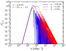
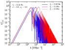
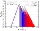
Figure 16: Filter functions $F_{K,12}^{2}$ (left), $F_{S,12}^{2}$ (middle), and $F_{K,12}F_{S,12}$ (right) used for calculations of auto and cross lensing dispersions (equations 40, 42, 44). $F_{K,12}$ and $F_{S,12}$ are defined in Equations (41) and (43), respectively. In all panels, we fix redshift $z=0.5$ and $z_{\rm s}=1$, and frequency $f_{1}=0.01$ Hz, and consider three different frequency $f_{2}$, $f_{2}=0.02$ Hz (solid), $0.1$ Hz (dashed), and $0.5$ Hz (dotted).

In practice, $K(f)$ and $S(f)$ have to be measured by comparing signals at different frequencies. For example, in an ideal case where the model waveform $h^{\rm model}(f)$ without gravitational lensing effects is completely known the following ratio between frequencies $f_{1}$ and $f_{2}$ reduces to

$$\frac{h(f_{1})/h^{\rm model}(f_{1})}{h(f_{2})/h^{\rm model}(f_{2})}\approx 1+K(f_{1})-K(f_{2})+i\left[S(f_{1})-S(f_{2})\right],$$ (C31)

from which we can measure auto and cross correlations of the differences of $K(f)$ and $S(f)$. After some calculations, they are found to be given by Equations (40), (42), and (44). We show examples of filter functions used for these calculations in Figure 16.

Appendix D Convergence and Magnification by the Shot Noise

We discuss the connection between lensing effects by individual point mass lenses and the variance of the convergence computed by the shot noise power spectrum. Specifically we consider a population of point mass lenses with their individual mass $m_{\rm p}$, the comoving number density $\bar{n}_{\rm p}$, and the mass fraction $m_{\rm p}\bar{n}_{\rm p}/\bar{\rho}=f_{\rm p}$. The shot noise contribution to the convergence variance smoothed over a circle with radius $\beta_{\rm s}$ is

$$\langle\kappa^{2}_{\rm shot}\rangle=\int d\chi W^{2}(\chi)\int\frac{k\,dk}{2\pi}\Delta P_{\rm shot}(k)W_{\rm s}^{2}(k\chi\beta_{\rm s}),$$ (D1)

where the lensing weight function $W(\chi)$ is defined in Equation (31) and $W_{\rm s}(x)$ is a smoothing kernel defined in Equation (32). The shot noise contribution to the matter power spectrum is given by

$$\Delta P_{\rm shot}(k)=\frac{f_{\rm p}^{2}}{\bar{n}_{\rm p}}.$$ (D2)

The lensing weight function is also rewritten as

$$W(\chi)=\frac{4\pi G\bar{\rho}a^{-1}\chi(\chi_{\rm s}-\chi)}{c^{2}\chi_{\rm s}}=\frac{\bar{\rho}a^{-2}}{\Sigma_{\rm crit}}=\pi R_{\rm Ein}^{2}\frac{\bar{n}_{\rm p}}{f_{\rm p}},$$ (D3)

where the comoving Einstein radius $R_{\rm Ein}$ for a point mass lens is given by

$$R_{\rm Ein}=\chi\theta_{\rm Ein}=\frac{1}{a}\sqrt{\frac{m_{\rm p}}{\pi\Sigma_{\rm crit}}}.$$ (D4)

By combining these calculations, we obtain

$$\langle\kappa^{2}_{\rm shot}\rangle=\int d\chi\frac{(\pi R_{\rm Ein}^{2})^{2}\bar{n}_{\rm p}}{\pi(\chi\beta_{\rm s})^{2}}=\sum\kappa_{\rm s}^{2}(\beta_{\rm s})\langle N_{\rm p}^{2}\rangle,$$ (D5)

where

$$\kappa_{\rm s}(\beta_{\rm s})=\left(\frac{R_{\rm Ein}}{\chi\beta_{\rm s}}\right)^{2},$$ (D6)

is the smoothed convergence for each point mass lens and

$$\langle N_{\rm p}^{2}\rangle=\pi(\chi\beta_{\rm s})^{2}\bar{n}_{\rm p}\Delta\chi$$ (D7)

is the variance of the number of point mass lenses within $\beta_{\rm s}$, which are assumed to be randomly distributed, within the radial distance slice $\Delta\chi$.

The discussion above suggests that the weak lensing approximation ($\mu_{\rm s}\approx 1+2\kappa_{\rm s}$) breaks down at $\chi\beta_{\rm s}\lesssim R_{\rm Ein}$, where $R_{\rm Ein}\sim 10^{-8}$ Mpc for $m_{\rm p}=1\leavevmode\nobreak\ M_{\odot}$, $z_{\rm s}=1$ and $z=0.5$.

For gravitational wave sources, the Fresnel scale $r_{\rm F}$ (equation 39) should be interpreted as the effective size of the source. Given the difference of the top-hat filter used above and the filter used to define the convergence of gravitational waves in Equation (35), we connect $\beta_{\rm s}$ with $r_{\rm F}$ as

$$\int\frac{k\,dk}{2\pi}F_{K}^{2}=\int\frac{k\,dk}{2\pi}W_{\rm s}^{2}(k\chi\beta_{\rm s}),$$ (D8)

where $F_{K}$ is defined in Equation (36). By solving this equation we find $(\chi\beta_{\rm s})^{2}/r_{\rm F}^{2}=4/\pi$. Thus the smoothed convergence (equation D6) is rewritten as

$$\kappa_{\rm s}=\frac{\pi}{4}\left(\frac{R_{\rm Ein}}{r_{\rm F}}\right)^{2}=\frac{\pi}{4}2\pi f(1+z)\frac{4Gm_{\rm p}}{c^{3}}=\frac{\pi}{4}w,$$ (D9)

where $w$ denotes the dimensionless parameter that controls the wave optics effect in gravitational lensing (see e.g., Oguri, 2019). The smoothed convergence can also be derived by directly evaluating $\delta\phi_{\rm obs}(f)/\phi_{\rm obs}^{0}(f)$ in the Born approximation for the case of a point mass lens (Takahashi et al., 2005)

$$\frac{\delta\phi_{\rm obs}(f)}{\phi_{\rm obs}^{0}(f)}=\frac{i}{2}w\left[{\rm Ci}\left(w\frac{R_{\perp}^{2}}{2R_{\rm Ein}^{2}}\right)+i\left\{{\rm Si}\left(w\frac{R_{\perp}^{2}}{2R_{\rm Ein}^{2}}\right)-\frac{\pi}{2}\right\}\right],$$ (D10)

where $R_{\perp}$ denote the comoving impact parameter at the lens. From this expression we can read off the smoothed convergence as

$$\kappa_{\rm s}={\rm Re}\left[\frac{\delta\phi_{\rm obs}(f)}{\phi_{\rm obs}^{0}(f)}\right]\approx\frac{\pi}{4}w\;\;\;(R_{\perp}\lesssim r_{\rm F}),$$ (D11)

which is consistent with Equation (D9).

On the other hand, using the $w$ parameter, the magnification factor of a point mass lens with the comoving impact parameter $R_{\perp}$ in the wave optics limit is described as (Deguchi & Watson, 1986a, b)

$$\mu_{\rm s}=\frac{\pi w}{1-e^{-\pi w}}\left|{}_{1}F_{1}\left(\frac{i}{2}w,1;\frac{i}{2}w\frac{R_{\perp}^{2}}{R_{\rm Ein}^{2}}\right)\right|^{2}\approx 1+\frac{\pi}{2}w\;\;\;(w\ll 1,\,R_{\perp}\lesssim r_{\rm F}),$$ (D12)

where ${}_{1}F_{1}$ is the confluent hypergeometric function. Hence the weak lensing relation $\mu_{\rm s}\approx 1+2\kappa_{\rm s}$ holds also for the case of the wave optics lensing by a point mass lens.

References

- Abbott et al. (2016) Abbott, B. P., Abbott, R., Abbott, T. D., et al. 2016, Phys. Rev. Lett., 116, 061102, doi: 10.1103/PhysRevLett.116.061102
- Afshordi et al. (2003) Afshordi, N., McDonald, P., & Spergel, D. N. 2003, ApJ, 594, L71, doi: 10.1086/378763
- Agrawal et al. (2019) Agrawal, A., Okumura, T., & Futamase, T. 2019, Phys. Rev. D, 100, 063534, doi: 10.1103/PhysRevD.100.063534
- Alam et al. (2017) Alam, S., Ata, M., Bailey, S., et al. 2017, MNRAS, 470, 2617, doi: 10.1093/mnras/stx721
- Ando et al. (2019) Ando, S., Ishiyama, T., & Hiroshima, N. 2019, Galaxies, 7, 68, doi: 10.3390/galaxies7030068
- Baltz et al. (2009) Baltz, E. A., Marshall, P., & Oguri, M. 2009, J. Cosmology Astropart. Phys, 2009, 015, doi: 10.1088/1475-7516/2009/01/015
- Banik et al. (2019) Banik, N., Bovy, J., Bertone, G., Erkal, D., & de Boer, T. J. L. 2019, arXiv e-prints, arXiv:1911.02663. https://arxiv.org/abs/1911.02663
- Battaglieri et al. (2017) Battaglieri, M., Belloni, A., Chou, A., et al. 2017, arXiv e-prints, arXiv:1707.04591. https://arxiv.org/abs/1707.04591
- Behroozi et al. (2019) Behroozi, P., Wechsler, R. H., Hearin, A. P., & Conroy, C. 2019, MNRAS, 488, 3143, doi: 10.1093/mnras/stz1182
- Ben-Dayan & Kalaydzhyan (2014) Ben-Dayan, I., & Kalaydzhyan, T. 2014, Phys. Rev. D, 90, 083509, doi: 10.1103/PhysRevD.90.083509
- Ben-Dayan & Takahashi (2016) Ben-Dayan, I., & Takahashi, R. 2016, MNRAS, 455, 552, doi: 10.1093/mnras/stv2356
- Bernardeau et al. (1997) Bernardeau, F., van Waerbeke, L., & Mellier, Y. 1997, A&A, 322, 1. https://arxiv.org/abs/astro-ph/9609122
- Blumenthal et al. (1984) Blumenthal, G. R., Faber, S. M., Primack, J. R., & Rees, M. J. 1984, Nature, 311, 517, doi: 10.1038/311517a0
- Bond et al. (1991) Bond, J. R., Cole, S., Efstathiou, G., & Kaiser, N. 1991, ApJ, 379, 440, doi: 10.1086/170520
- Bovy et al. (2017) Bovy, J., Erkal, D., & Sanders, J. L. 2017, MNRAS, 466, 628, doi: 10.1093/mnras/stw3067
- Bower (1991) Bower, R. G. 1991, MNRAS, 248, 332, doi: 10.1093/mnras/248.2.332
- Bullock & Boylan-Kolchin (2017) Bullock, J. S., & Boylan-Kolchin, M. 2017, ARA&A, 55, 343, doi: 10.1146/annurev-astro-091916-055313
- Carr et al. (2020) Carr, B., Kohri, K., Sendouda, Y., & Yokoyama, J. 2020, arXiv e-prints, arXiv:2002.12778. https://arxiv.org/abs/2002.12778
- Chisari et al. (2019) Chisari, N. E., Mead, A. J., Joudaki, S., et al. 2019, The Open Journal of Astrophysics, 2, 4, doi: 10.21105/astro.1905.06082
- Cooray & Sheth (2002) Cooray, A., & Sheth, R. 2002, Phys. Rep., 372, 1, doi: 10.1016/S0370-1573(02)00276-4
- Dai et al. (2018a) Dai, L., Li, S.-S., Zackay, B., Mao, S., & Lu, Y. 2018a, Phys. Rev. D, 98, 104029, doi: 10.1103/PhysRevD.98.104029
- Dai & Miralda-Escudé (2020) Dai, L., & Miralda-Escudé, J. 2020, AJ, 159, 49, doi: 10.3847/1538-3881/ab5e83
- Dai et al. (2018b) Dai, L., Venumadhav, T., Kaurov, A. A., & Miralda-Escud, J. 2018b, ApJ, 867, 24, doi: 10.3847/1538-4357/aae478
- Davis et al. (1985) Davis, M., Efstathiou, G., Frenk, C. S., & White, S. D. M. 1985, ApJ, 292, 371, doi: 10.1086/163168
- Debackere et al. (2020) Debackere, S. N. B., Schaye, J., & Hoekstra, H. 2020, MNRAS, 492, 2285, doi: 10.1093/mnras/stz3446
- Deguchi & Watson (1986a) Deguchi, S., & Watson, W. D. 1986a, ApJ, 307, 30, doi: 10.1086/164389
- Deguchi & Watson (1986b) —. 1986b, Phys. Rev. D, 34, 1708, doi: 10.1103/PhysRevD.34.1708
- Diemer & Joyce (2019) Diemer, B., & Joyce, M. 2019, ApJ, 871, 168, doi: 10.3847/1538-4357/aafad6
- Diemer & Kravtsov (2015) Diemer, B., & Kravtsov, A. V. 2015, ApJ, 799, 108, doi: 10.1088/0004-637X/799/1/108
- Dodelson & Vallinotto (2006) Dodelson, S., & Vallinotto, A. 2006, Phys. Rev. D, 74, 063515, doi: 10.1103/PhysRevD.74.063515
- Dror et al. (2019) Dror, J. A., Ramani, H., Trickle, T., & Zurek, K. M. 2019, Phys. Rev. D, 100, 023003, doi: 10.1103/PhysRevD.100.023003
- Fedeli (2014) Fedeli, C. 2014, J. Cosmology Astropart. Phys, 2014, 028, doi: 10.1088/1475-7516/2014/04/028
- Fedeli & Moscardini (2014) Fedeli, C., & Moscardini, L. 2014, MNRAS, 442, 2659, doi: 10.1093/mnras/stu1043
- Fedeli et al. (2014) Fedeli, C., Semboloni, E., Velliscig, M., et al. 2014, J. Cosmology Astropart. Phys, 2014, 028, doi: 10.1088/1475-7516/2014/08/028
- Gilman et al. (2020) Gilman, D., Birrer, S., Nierenberg, A., et al. 2020, MNRAS, 491, 6077, doi: 10.1093/mnras/stz3480
- Giocoli et al. (2010) Giocoli, C., Bartelmann, M., Sheth, R. K., & Cacciato, M. 2010, MNRAS, 408, 300, doi: 10.1111/j.1365-2966.2010.17108.x
- Giocoli et al. (2007) Giocoli, C., Moreno, J., Sheth, R. K., & Tormen, G. 2007, MNRAS, 376, 977, doi: 10.1111/j.1365-2966.2007.11520.x
- Giocoli et al. (2008a) Giocoli, C., Pieri, L., & Tormen, G. 2008a, MNRAS, 387, 689, doi: 10.1111/j.1365-2966.2008.13283.x
- Giocoli et al. (2008b) Giocoli, C., Tormen, G., & van den Bosch, F. C. 2008b, MNRAS, 386, 2135, doi: 10.1111/j.1365-2966.2008.13182.x
- Gong & Kitajima (2017) Gong, J.-O., & Kitajima, N. 2017, J. Cosmology Astropart. Phys, 2017, 017, doi: 10.1088/1475-7516/2017/08/017
- Hada & Futamase (2016) Hada, R., & Futamase, T. 2016, ApJ, 828, 112, doi: 10.3847/0004-637X/828/2/112
- Hada & Futamase (2019) —. 2019, J. Cosmology Astropart. Phys, 2019, 033, doi: 10.1088/1475-7516/2019/06/033
- Hamana & Futamase (2000) Hamana, T., & Futamase, T. 2000, ApJ, 534, 29, doi: 10.1086/308758
- Han et al. (2016) Han, J., Cole, S., Frenk, C. S., & Jing, Y. 2016, MNRAS, 457, 1208, doi: 10.1093/mnras/stv2900
- Hernquist (1990) Hernquist, L. 1990, ApJ, 356, 359, doi: 10.1086/168845
- Hiroshima et al. (2018) Hiroshima, N., Ando, S., & Ishiyama, T. 2018, Phys. Rev. D, 97, 123002, doi: 10.1103/PhysRevD.97.123002
- Holz & Hughes (2005) Holz, D. E., & Hughes, S. A. 2005, ApJ, 629, 15, doi: 10.1086/431341
- Huang et al. (2017) Huang, K.-H., Fall, S. M., Ferguson, H. C., et al. 2017, ApJ, 838, 6, doi: 10.3847/1538-4357/aa62a6
- Ibata et al. (2002) Ibata, R. A., Lewis, G. F., Irwin, M. J., & Quinn, T. 2002, MNRAS, 332, 915, doi: 10.1046/j.1365-8711.2002.05358.x
- Inman & Ali-Haïmoud (2019) Inman, D., & Ali-Haïmoud, Y. 2019, Phys. Rev. D, 100, 083528, doi: 10.1103/PhysRevD.100.083528
- Inoue & Chiba (2003) Inoue, K. T., & Chiba, M. 2003, ApJ, 591, L83, doi: 10.1086/377247
- Inoue et al. (2015) Inoue, K. T., Takahashi, R., Takahashi, T., & Ishiyama, T. 2015, MNRAS, 448, 2704, doi: 10.1093/mnras/stv194
- Ishiyama & Ando (2020) Ishiyama, T., & Ando, S. 2020, MNRAS, 492, 3662, doi: 10.1093/mnras/staa069
- Jiang & van den Bosch (2016) Jiang, F., & van den Bosch, F. C. 2016, MNRAS, 458, 2848, doi: 10.1093/mnras/stw439
- Jönsson et al. (2007) Jönsson, J., Dahlén, T., Goobar, A., Mörtsell, E., & Riess, A. 2007, J. Cosmology Astropart. Phys, 2007, 002, doi: 10.1088/1475-7516/2007/06/002
- Jönsson et al. (2010) Jönsson, J., Sullivan, M., Hook, I., et al. 2010, MNRAS, 405, 535, doi: 10.1111/j.1365-2966.2010.16467.x
- Karpenka et al. (2013) Karpenka, N. V., March, M. C., Feroz, F., & Hobson, M. P. 2013, MNRAS, 433, 2693, doi: 10.1093/mnras/sts700
- Kashiyama & Oguri (2018) Kashiyama, K., & Oguri, M. 2018, arXiv e-prints, arXiv:1801.07847. https://arxiv.org/abs/1801.07847
- Kawamata et al. (2015) Kawamata, R., Ishigaki, M., Shimasaku, K., Oguri, M., & Ouchi, M. 2015, ApJ, 804, 103, doi: 10.1088/0004-637X/804/2/103
- Kawamata et al. (2018) Kawamata, R., Ishigaki, M., Shimasaku, K., et al. 2018, ApJ, 855, 4, doi: 10.3847/1538-4357/aaa6cf
- Kelly et al. (2018) Kelly, P. L., Diego, J. M., Rodney, S., et al. 2018, Nature Astronomy, 2, 334, doi: 10.1038/s41550-018-0430-3
- Koopmans (2005) Koopmans, L. V. E. 2005, MNRAS, 363, 1136, doi: 10.1111/j.1365-2966.2005.09523.x
- Kravtsov (2013) Kravtsov, A. V. 2013, ApJ, 764, L31, doi: 10.1088/2041-8205/764/2/L31
- Kravtsov et al. (2018) Kravtsov, A. V., Vikhlinin, A. A., & Meshcheryakov, A. V. 2018, Astronomy Letters, 44, 8, doi: 10.1134/S1063773717120015
- Kronborg et al. (2010) Kronborg, T., Hardin, D., Guy, J., et al. 2010, A&A, 514, A44, doi: 10.1051/0004-6361/200913618
- Lacey & Cole (1993) Lacey, C., & Cole, S. 1993, MNRAS, 262, 627, doi: 10.1093/mnras/262.3.627
- Lee (2004) Lee, J. 2004, ApJ, 604, L73, doi: 10.1086/386304
- Lindblom et al. (2008) Lindblom, L., Owen, B. J., & Brown, D. A. 2008, Phys. Rev. D, 78, 124020, doi: 10.1103/PhysRevD.78.124020
- Macquart (2004) Macquart, J. P. 2004, A&A, 422, 761, doi: 10.1051/0004-6361:20034512
- Mao & Schneider (1998) Mao, S., & Schneider, P. 1998, MNRAS, 295, 587, doi: 10.1046/j.1365-8711.1998.01319.x
- Marinacci et al. (2018) Marinacci, F., Vogelsberger, M., Pakmor, R., et al. 2018, MNRAS, 480, 5113, doi: 10.1093/mnras/sty2206
- Mediavilla et al. (2017) Mediavilla, E., Jiménez-Vicente, J., Muñoz, J. A., Vives-Arias, H., & Calderón-Infante, J. 2017, ApJ, 836, L18, doi: 10.3847/2041-8213/aa5dab
- Metcalf (1999) Metcalf, R. B. 1999, MNRAS, 305, 746, doi: 10.1046/j.1365-8711.1999.02382.x
- Mo et al. (2010) Mo, H., van den Bosch, F. C., & White, S. 2010, Galaxy Formation and Evolution
- Moliné et al. (2017) Moliné, Á., Sánchez-Conde, M. A., Palomares-Ruiz, S., & Prada, F. 2017, MNRAS, 466, 4974, doi: 10.1093/mnras/stx026
- Mondino et al. (2020) Mondino, C., Taki, A.-M., Van Tilburg, K., & Weiner, N. 2020, arXiv e-prints, arXiv:2002.01938. https://arxiv.org/abs/2002.01938
- Naiman et al. (2018) Naiman, J. P., Pillepich, A., Springel, V., et al. 2018, MNRAS, 477, 1206, doi: 10.1093/mnras/sty618
- Nakamura et al. (2016) Nakamura, T., Ando, M., Kinugawa, T., et al. 2016, Progress of Theoretical and Experimental Physics, 2016, 093E01, doi: 10.1093/ptep/ptw127
- Nakamura & Deguchi (1999) Nakamura, T. T., & Deguchi, S. 1999, Progress of Theoretical Physics Supplement, 133, 137, doi: 10.1143/PTPS.133.137
- Nakamura & Suto (1997) Nakamura, T. T., & Suto, Y. 1997, Progress of Theoretical Physics, 97, 49, doi: 10.1143/PTP.97.49
- Navarro et al. (1997) Navarro, J. F., Frenk, C. S., & White, S. D. M. 1997, ApJ, 490, 493, doi: 10.1086/304888
- Nelson et al. (2018) Nelson, D., Pillepich, A., Springel, V., et al. 2018, MNRAS, 475, 624, doi: 10.1093/mnras/stx3040
- Oguri (2018) Oguri, M. 2018, MNRAS, 480, 3842, doi: 10.1093/mnras/sty2145
- Oguri (2019) —. 2019, Reports on Progress in Physics, 82, 126901, doi: 10.1088/1361-6633/ab4fc5
- Oguri et al. (2018) Oguri, M., Diego, J. M., Kaiser, N., Kelly, P. L., & Broadhurst, T. 2018, Phys. Rev. D, 97, 023518, doi: 10.1103/PhysRevD.97.023518
- Oguri & Hamana (2011) Oguri, M., & Hamana, T. 2011, MNRAS, 414, 1851, doi: 10.1111/j.1365-2966.2011.18481.x
- Oguri & Lee (2004) Oguri, M., & Lee, J. 2004, MNRAS, 355, 120, doi: 10.1111/j.1365-2966.2004.08304.x
- Peebles (1982) Peebles, P. J. E. 1982, ApJ, 263, L1, doi: 10.1086/183911
- Pillepich et al. (2018) Pillepich, A., Nelson, D., Hernquist, L., et al. 2018, MNRAS, 475, 648, doi: 10.1093/mnras/stx3112
- Planck Collaboration et al. (2016) Planck Collaboration, Ade, P. A. R., Aghanim, N., et al. 2016, A&A, 594, A13, doi: 10.1051/0004-6361/201525830
- Quartin et al. (2014) Quartin, M., Marra, V., & Amendola, L. 2014, Phys. Rev. D, 89, 023009, doi: 10.1103/PhysRevD.89.023009
- Quimby et al. (2014) Quimby, R. M., Oguri, M., More, A., et al. 2014, Science, 344, 396, doi: 10.1126/science.1250903
- Ritondale et al. (2019) Ritondale, E., Vegetti, S., Despali, G., et al. 2019, MNRAS, 485, 2179, doi: 10.1093/mnras/stz464
- Sasaki et al. (2018) Sasaki, M., Suyama, T., Tanaka, T., & Yokoyama, S. 2018, Classical and Quantum Gravity, 35, 063001, doi: 10.1088/1361-6382/aaa7b4
- Schutz (1986) Schutz, B. F. 1986, Nature, 323, 310, doi: 10.1038/323310a0
- Semboloni et al. (2011) Semboloni, E., Hoekstra, H., Schaye, J., van Daalen, M. P., & McCarthy, I. G. 2011, MNRAS, 417, 2020, doi: 10.1111/j.1365-2966.2011.19385.x
- Seto et al. (2001) Seto, N., Kawamura, S., & Nakamura, T. 2001, Phys. Rev. Lett., 87, 221103, doi: 10.1103/PhysRevLett.87.221103
- Sheth & Tormen (1999) Sheth, R. K., & Tormen, G. 1999, MNRAS, 308, 119, doi: 10.1046/j.1365-8711.1999.02692.x
- Smith et al. (2014) Smith, M., Bacon, D. J., Nichol, R. C., et al. 2014, ApJ, 780, 24, doi: 10.1088/0004-637X/780/1/24
- Smith et al. (2003) Smith, R. E., Peacock, J. A., Jenkins, A., et al. 2003, MNRAS, 341, 1311, doi: 10.1046/j.1365-8711.2003.06503.x
- Springel et al. (2018) Springel, V., Pakmor, R., Pillepich, A., et al. 2018, MNRAS, 475, 676, doi: 10.1093/mnras/stx3304
- Takahashi (2006) Takahashi, R. 2006, ApJ, 644, 80, doi: 10.1086/503323
- Takahashi et al. (2011) Takahashi, R., Oguri, M., Sato, M., & Hamana, T. 2011, ApJ, 742, 15, doi: 10.1088/0004-637X/742/1/15
- Takahashi et al. (2012) Takahashi, R., Sato, M., Nishimichi, T., Taruya, A., & Oguri, M. 2012, ApJ, 761, 152, doi: 10.1088/0004-637X/761/2/152
- Takahashi et al. (2005) Takahashi, R., Suyama, T., & Michikoshi, S. 2005, A&A, 438, L5, doi: 10.1051/0004-6361:200500140
- van den Bosch et al. (2005) van den Bosch, F. C., Tormen, G., & Giocoli, C. 2005, MNRAS, 359, 1029, doi: 10.1111/j.1365-2966.2005.08964.x
- Van Tilburg et al. (2018) Van Tilburg, K., Taki, A.-M., & Weiner, N. 2018, J. Cosmology Astropart. Phys, 2018, 041, doi: 10.1088/1475-7516/2018/07/041
- Vegetti et al. (2012) Vegetti, S., Lagattuta, D. J., McKean, J. P., et al. 2012, Nature, 481, 341, doi: 10.1038/nature10669
- White (2004) White, M. 2004, Astroparticle Physics, 22, 211, doi: 10.1016/j.astropartphys.2004.06.001
- Zanisi et al. (2020) Zanisi, L., Shankar, F., Lapi, A., et al. 2020, MNRAS, 492, 1671, doi: 10.1093/mnras/stz3516
- Zhan & Knox (2004) Zhan, H., & Knox, L. 2004, ApJ, 616, L75, doi: 10.1086/426712
- Zumalacárregui & Seljak (2018) Zumalacárregui, M., & Seljak, U. 2018, Phys. Rev. Lett., 121, 141101, doi: 10.1103/PhysRevLett.121.141101