Efficient Marginalization of
Discrete and Structured Latent Variables via Sparsity

Abstract

Training neural network models with discrete (categorical or structured) latent variables can be computationally challenging, due to the need for marginalization over large or combinatorial sets. To circumvent this issue, one typically resorts to sampling-based approximations of the true marginal, requiring noisy gradient estimators (e.g., score function estimator) or continuous relaxations with lower-variance reparameterized gradients (e.g., Gumbel-Softmax). In this paper, we propose a new training strategy which replaces these estimators by an exact yet efficient marginalization. To achieve this, we parameterize discrete distributions over latent assignments using differentiable sparse mappings: sparsemax and its structured counterparts. In effect, the support of these distributions is greatly reduced, which enables efficient marginalization. We report successful results in three tasks covering a range of latent variable modeling applications: a semisupervised deep generative model, a latent communication game, and a generative model with a bit-vector latent representation. In all cases, we obtain good performance while still achieving the practicality of sampling-based approximations.

1 Introduction

Neural latent variable models are powerful and expressive tools for finding patterns in high-dimensional data, such as images or text [1, 2, 3]. Of particular interest are discrete latent variables, which can recover categorical and structured encodings of hidden aspects of the data, leading to compact representations and, in some cases, superior explanatory power [4, 5]. However, with discrete variables, training can become challenging, due to the need to compute a gradient of a large sum over all possible latent variable assignments, with each term itself being potentially expensive. This challenge is typically tackled by estimating the gradient with Monte Carlo methods [MC; 6], which rely on sampling estimates. The two most common strategies for MC gradient estimation are the score function estimator [SFE; 7, 8], which suffers from high variance, or surrogate methods that rely on the continuous relaxation of the latent variable, like straight-through [9] or Gumbel-Softmax [10, 11] which potentially reduce variance but introduce bias and modeling assumptions.

In this work, we take a step back and ask: Can we avoid sampling entirely, and instead deterministically evaluate the sum with less computation? To answer affirmatively, we propose an alternative method to train these models by parameterizing the discrete distribution with sparse mappings — sparsemax [12] and two structured counterparts, SparseMAP [13] and a novel mapping top-$k$ sparsemax. Sparsity implies that some assignments of the latent variable are entirely ruled out. This leads to the corresponding terms in the sum evaluating trivially to zero, allowing us to disregard potentially expensive computations.

Contributions.

We introduce a general strategy for learning deep models with discrete latent variables that hinges on learning a sparse distribution over the possible assignments. In the unstructured categorical case our strategy relies on the sparsemax activation function, presented in §3, while in the structured case we propose two strategies, SparseMAP and top-$k$ sparsemax, presented in §4. Unlike existing approaches, our strategies involve neither MC estimation nor any relaxation of the discrete latent variable to the continuous space. We demonstrate our strategy on three different applications: a semisupervised generative model, an emergent communication game, and a bit-vector variational autoencoder. We provide a thorough analysis and comparison to MC methods, and — when feasible — to exact marginalization. Our approach is consistently a top performer, combining the accuracy and robustness of exact marginalization with the efficiency of single-sample estimators.

Notation.

We denote scalars, vectors, matrices, and sets as $a$, $\bm{a}$, $\bm{A}$, and $\mathcal{A}$, respectively. The indicator vector is denoted by $\bm{e}_{i}$, for which every entry is zero, except the $i$^th, which is 1. The simplex is denoted $\triangle^{K}\coloneqq\{\bm{\xi}\in\mathbb{R}^{K}~{}:~{}\langle\bm{1},\bm{\xi}\rangle=1,\bm{\xi}\geq\bm{0}\}$. $\mathbb{H}(p)$ denotes the Shannon entropy of a distribution $p(z)$, and $\operatorname{\mathsf{KL}}\left[p||q\right]$ denotes the Kullback-Leibler divergence of $p(z)$ from $q(z)$. The number of non-zeros of a sequence $z$ is denoted $\|z\|_{0}\coloneqq|\{t:z_{t}\neq 0\}|$. Letting $z\in\mathcal{Z}$ be a random variable, we write the expectation of a function $f:\mathcal{Z}\rightarrow\mathbb{R}$ under distribution $p(z)$ as $\mathbb{E}_{p(z)}[f(z)]$.

2 Background

We assume throughout a latent variable model with observed variables $x\in\mathcal{X}$ and latent stochastic variables $z\in\mathcal{Z}$. The overall fit to a dataset $\mathcal{D}$ is $\sum_{x\in\mathcal{D}}\mathcal{L}_{x}(\theta)$, where the loss of each observation,

$$\mathcal{L}_{x}(\theta)=\mathbb{E}_{\pi(z\mid x,\theta)}\left[\ell(x,z;\theta)\right]=\sum_{z\in\mathcal{Z}}\pi(z|x,\theta)~{}\ell(x,z;\theta)~{},$$ (1)

is the expected value of a downstream loss $\ell(x,z;\theta)$ under a probability model $\pi(z|x,\theta)$ of the latent variable; in other words, the latent variable $z$ is marginalized to compute this loss. To model complex data, one parameterizes both the downstream loss and the distribution over latent assignments using neural networks, due to their flexibility and capacity [2].

In this work, we study discrete latent variables, where $|\mathcal{Z}|$ is finite, but possibly very large. One example is when $\pi(z|x,\theta)$ is a categorical distribution, parameterized by a vector $\bm{\xi}\in\triangle^{|\mathcal{Z}|}$. To obtain $\bm{\xi}$, a neural network computes a vector of scores $\bm{s}\in\mathbb{R}^{|\mathcal{Z}|}$, one score for each assignment, which is then mapped to the probability simplex, typically via $\bm{\xi}=\operatorname*{\mathsf{softmax}}(\bm{s})$. Another example is when $\mathcal{Z}$ is a structured (combinatorial) set, such as $\mathcal{Z}=\{0,1\}^{D}$. In this case, $|\mathcal{Z}|$ grows exponentially with $D$ and it is infeasible to enumerate and score all possible assignments. For this structured case, scoring assignments involves a decomposition into parts, which we describe in §4.

Training such models requires summing the contributions of all assignments of the latent variable, which involves as many as $|\mathcal{Z}|$ evaluations of the downstream loss. When $\mathcal{Z}$ is not too large, the expectation may be evaluated explicitly, and learning can proceed with exact gradient updates. If $\mathcal{Z}$ is large, and/or if $\ell$ is an expensive computation, evaluating the expectation becomes prohibitive. In such cases, practitioners typically turn to MC estimates of $\nabla_{\theta}\mathcal{L}_{x}(\theta)$ derived from latent assignments sampled from $\pi(z|x,\theta)$. Under an appropriate learning rate schedule, this procedure converges to a local optimum of $\mathcal{L}_{x}(\theta)$ as long as gradient estimates are unbiased [14]. Next, we describe the two current main strategies for MC estimation of this gradient. Later, in §3–4, we propose our deterministic alternative, based on sparsifying $\pi(z|x,\theta)$.

Monte Carlo gradient estimates.

Let $\theta=(\theta_{\pi},\theta_{\ell})$, where $\theta_{\pi}$ is the subset of weights that $\pi$ depends on, and $\theta_{\ell}$ the subset of weights that $\ell$ depends on. Given a sample $z\sim\pi(z|x,\theta_{\pi})$, an unbiased estimator of the gradient for Eq. 1 w. r. t. $\theta_{\ell}$ is $\nabla_{\theta_{\ell}}\mathcal{L}_{x}(\theta)\approx\nabla_{\theta_{\ell}}\ell(x,z;\theta_{\ell})$. Unbiased estimation of $\nabla_{\theta_{\pi}}\mathcal{L}_{x}(\theta)$ is more difficult, since $\theta_{\pi}$ is involved in the sampling of $z$, but can be done with SFE [7, 8]: $\nabla_{\theta_{\pi}}\mathcal{L}_{x}(\theta)\approx\ell(x,z;\theta_{\ell})~{}\nabla_{\theta_{\pi}}\operatorname*{\mathsf{log}}\pi(z|x,\theta_{\pi})$, also known as reinforce [15]. The SFE is powerful and general, making no assumptions on the form of $z$ or $\ell$, requiring only a sampling oracle and a way to assess gradients of $\operatorname*{\mathsf{log}}\pi(z|x,\theta_{\pi})$. However, it comes with the cost of high variance. Making the estimator practically useful requires variance reduction techniques such as baselines [15, 16] and control variates [17, 18, 19]. Variance reduction can also be achieved with Rao-Blackwellization techniques such as sum and sample [20, 21, 22], which marginalizes an expectation over the top-$k$ elements of $\pi(z|x,\theta_{\pi})$ and takes a sample estimate from the complement set.

Reparameterization trick.

For continuous latent variables, low-variance pathwise gradient estimators can be obtained by separating the source of stochasticity from the sampling parameters, using the so-called reparameterization trick [2, 3]. For discrete latent variables, reparameterizations can only be obtained by introducing a step function like $\operatorname*{\mathsf{argmax}}$, which has null gradients almost everywhere. Replacing the gradient of $\operatorname*{\mathsf{argmax}}$ with a nonzero surrogate like the identity function, known as Straight-Through [9], or with the gradient of $\operatorname*{\mathsf{softmax}}$, known as Gumbel-Softmax [10, 11], leads to a biased estimator that can still perform well in practice. Continuous relaxations like Straight-Through and Gumbel-Softmax are only possible under a further modeling assumption that $\ell$ is defined continuously (thus differentiably) in a neighbourhood of the indicator vector $\bm{z}=\bm{e}_{z}$ for every $z\in\mathcal{Z}$. In contrast, both SFE-based methods as well as our approach make no such assumption.

3 Efficient Marginalization via Sparsity

The challenge of computing the exact expectation in Eq. 1 is linked to the need to compute a sum with a large number of terms. This holds when the probability distribution over latent assignments is dense (i.e., every assignment $z\in\mathcal{Z}$ has non-zero probability), which is indeed the case for most parameterizations of discrete distributions. Our proposed methods hinge on sparsifying this sum.

Take the example where $\mathcal{Z}=\{1,\ldots,K\}$, with a neural network predicting from $x$ a $K$-dimensional vector of real-valued scores $\bm{s}=\bm{g}(x;\theta)$, such that $s_{z}$ is the score of $z$. The traditional way to obtain the vector $\bm{\xi}$ parameterizing $\pi(z|x,\theta)$ is with the softmax transform, i. e. $\bm{\xi}=\operatorname*{\mathsf{softmax}}(\bm{s})$. Since this gives $\pi(z|x,\theta)\propto\operatorname*{\mathsf{exp}}(s_{z})$, the expectation in Eq. 1 depends on $\ell(x,z;\theta)$ for every possible $z$.

We rethink this standard parameterization, proposing a sparse mapping from scores to the simplex. In particular, we substitute softmax by sparsemax [12]:

$$\operatorname*{\mathsf{sparsemax}}(\bm{s})\coloneqq\operatorname*{\mathsf{argmin}}_{\bm{\xi}\in\triangle^{K}}\|\bm{\xi}-\bm{s}\|_{2}^{2}~{}.$$ (2)

Like softmax, sparsemax is differentiable and has efficient forward and backward passes [23, 12], described in detail in App. A; the backward pass is essential in our use case. Since Eq. 2 is the Euclidean projection operator onto the probability simplex, and solutions can hit the boundary, sparsemax is likely to assign probabilities of exactly zero; in contrast, softmax is always dense.

Our main insight is that with a sparse parameterization of $\pi$, we can compute the expectation in Eq. 1 evaluating $\ell(x,z;\theta)$ only for assignments $z\in\bar{\mathcal{Z}}\coloneqq\{z:\pi(z|x,\theta)>0\}$. This leads to a powerful alternative to MC estimation, which requires fewer than $|\mathcal{Z}|$ evaluations of $\ell$, and which strategically — yet deterministically — selects which assignments $\bar{\mathcal{Z}}$ to evaluate $\ell$ on. Empirically, our analysis in §5 reveals an adaptive behavior of this sparsity-inducing mechanism, performing more loss evaluations in early iterations while the model is uncertain, and quickly reducing the number of evaluations, especially for unambiguous data points. This is a notable property of our learning strategy: In contrast, MC estimation cannot decide when an ambiguous data point may require more sampling for accurate estimation; and directly evaluating Eq. 1 with the dense $\bm{\xi}$ resulting from a softmax parameterization never reduces the number of evaluations required, even for simple instances.

4 Structured Latent Variables

While the approach described in §3 theoretically applies to any discrete distribution, many models of interest involve structured (or combinatorial) latent variables. In this section, we assume $z$ can be represented as a bit-vector—i. e. a random vector of discrete binary variables $\bm{a}_{z}\in\{0,1\}^{D}$. This assignment of binary variables may involve global factors and constraints (e. g. tree constraints, or budget constraints on the number of active variables, i. e. $\sum_{i}[\bm{a}_{z}]_{i}\leq B$, where $B$ is the maximum number of variables allowed to activate at the same time). In such structured problems, $|\mathcal{Z}|$ increases exponentially with $D$, making exact evaluation of $\ell(x,z;\theta)$ prohibitive, even with sparsemax.

Structured prediction typically handles this combinatorial explosion by parameterizing scores for individual binary variables and interactions within the global structured configuration, yielding a compact vector of variable scores $\bm{t}=\bm{g}(x;\theta)\in\mathbb{R}^{D}$ (e. g., log-potentials for binary attributes), with $D\ll|\mathcal{Z}|$. Then, the score of some global configuration $z\in\mathcal{Z}$ is $s_{z}\coloneqq\langle\bm{a}_{z},\bm{t}\rangle$. The variable scores induce a unique Gibbs distribution over structures, given by $\pi(z|x,\theta)\propto\operatorname*{\mathsf{exp}}(\langle\bm{a}_{z},\bm{t}\rangle)$. Equivalently, defining $\bm{A}\in\mathbb{R}^{D\times|\mathcal{Z}|}$ as the matrix with columns $\bm{a}_{z}$ for all $z\in\mathcal{Z}$, we consider the discrete distribution parameterized by $\operatorname*{\mathsf{softmax}}(\bm{s})$, where $\bm{s}=\bm{A}^{\top}\bm{t}$. (In the unstructured case, $\bm{A}=\bm{I}$.)

In practice, however, we cannot materialize the matrix $\bm{A}$ or the global score vector $\bm{s}$, let alone compute the softmax and the sum in Eq. 1. The SFE, however, can still be used, provided that exact sampling of $z\sim\pi(z|x,\theta)$ is feasible, and efficient algorithms exist for computing the normalizing constant $\sum_{z^{\prime}}\operatorname*{\mathsf{exp}}(\langle\bm{a}_{z^{\prime}},\bm{t}\rangle)$ [24], needed to compute the probability of a given sample.

While it may be tempting to consider using sparsemax to avoid the expensive sum in the exact expectation, this is prohibitive too: solving the problem in Eq. 2 still requires explicit manipulation of the large vector $\bm{s}\in\mathbb{R}^{|\mathcal{Z}|}$, and even if we could avoid this, in the worst case ($\bm{s}=\bm{0}$) the resulting sparsemax distribution would still have exponentially large support. Fortunately, we show next that it is still possible to develop sparsification strategies to handle the combinatorial explosion of $\mathcal{Z}$ in the structured case. We propose two different methods to obtain a sparse distribution $\bm{\xi}$ supported only over a bounded-size subset of $\mathcal{Z}$: top-$k$ sparsemax (§4.1) and SparseMAP (§4.2).

4.1 Top-$k$ Sparsemax

Recall that the sparsemax operator (Eq. 2) is simply the Euclidean projection onto the $|\mathcal{Z}|$-dimensional probability simplex. While this projection has a propensity to be sparse, there is no upper bound on the number of non-zeros of the resulting distribution. When $\mathcal{Z}$ is large, one possibility is to add a cardinality constraint $\|\bm{\xi}\|_{0}\leq k$ for some prescribed $k\in\mathbb{N}$. The resulting problem becomes

$$\operatorname{\mathsf{sparsemax}_{\text{$k$}}}(\bm{s})\coloneqq\operatorname*{\mathsf{argmin}}_{\bm{\xi}\in\triangle^{|\mathcal{Z}|},\,\|\bm{\xi}\|_{0}\leq k}\|\bm{\xi}-\bm{s}\|_{2}^{2},$$ (3)

which is known as a sparse projection onto the simplex and has been studied in detail by Kyrillidis et al. [25] and used to smooth structured prediction losses [26, 27]. Remarkably, while this is a non-convex problem, its solution $\bm{\xi}^{\star}$ can be written as a composition of two functions: a top-$k$ operator $\operatorname{\mathsf{top}_{\text{$k$}}}:\mathbb{R}^{|\mathcal{Z}|}\rightarrow\mathbb{R}^{|\mathcal{Z}|}$, which returns a vector identical to its input but where all the entries not among the $k$ largest ones are masked out (set to $-\infty$), and the $k$-dimensional sparsemax operator.

Formally, $\operatorname{\mathsf{sparsemax}_{\text{$k$}}}=\operatorname*{\mathsf{sparsemax}}(\operatorname{\mathsf{top}_{\text{$k$}}}(\bm{s}))$. Being a composition of operators, its Jacobian becomes a product of matrices and hence simple to compute (the Jacobian of $\operatorname{\mathsf{top}_{\text{$k$}}}$ is a diagonal matrix whose diagonal is a multi-hot vector indicating the top-$k$ elements of $\bm{s}$).

To apply the top-$k$ sparsemax to a large or combinatorial set $\mathcal{Z}$, all we need is a primitive to compute the top-$k$ entries of $s$—this is available for many structured problems (for example, sequential models via $k$-best dynamic programming) and, when $\mathcal{Z}$ is the set of joint assignments of $D$ discrete binary variables, it can be done with a cost $\mathcal{O}(kD)$.

After enumerating this set, we parameterize $\pi(z|x,\theta)$ by applying sparsemax to that top-$k$, with a computational cost $\mathcal{O}(k)$. Note that this method is identical to sparsemax whenever $\|\operatorname*{\mathsf{sparsemax}}(\bm{s})\|_{0}\leq k$: if during training the model learns to assign a sparse distribution to the latent variable, we are effectively using a sparsemax parameterization as presented in §3 with cheap computation. In fact, the solution of Eq. 3 gives us a certificate of optimality whenever $\|\bm{\xi}^{\star}\|_{0}<k$.

4.2 SparseMAP

A second possibility to obtain efficient summation over a combinatorial space without imposing any constraints on $\ell(x,z;\theta)$ is to use SparseMAP [13, 28], a structured extension of sparsemax:

$$\operatorname*{\mathsf{SparseMAP}}(\bm{t})\coloneqq\operatorname*{\mathsf{argmin}}_{\bm{\xi}\in\triangle^{|\mathcal{Z}|}}\|\bm{A}\bm{\xi}-\bm{t}\|_{2}^{2},$$ (4)

SparseMAP has been used successfully in discriminative latent models to model structures such as trees and matchings, and Niculae et al. [13] apply an active set algorithm for evaluating it and computing gradients efficiently, requiring only a primitive for computing $\operatorname*{\mathsf{argmax}}_{z\in\mathcal{Z}}\langle\bm{a}_{z},\bm{t}\rangle$. (We detail the algorithm in App. B). While the $\operatorname*{\mathsf{argmin}}$ in (4) is generally not unique, Carathéodory’s theorem guarantees that solutions with support size at most $D+1$ exist, and the active set algorithm enjoys linear and finite convergence to a very sparse optimal distribution. Crucially, (4) has a solution $\bm{\xi}^{\star}$ such that the set $\bar{\mathcal{Z}}=\left\{z\in\mathcal{Z}\mid\xi^{\star}_{z}>0\right\}$ grows only linearly with $D$, and therefore $|\bar{\mathcal{Z}}|\ll|\mathcal{Z}|$. Therefore, assessing the expectation in Eq. 1 only requires evaluating $|\bar{\mathcal{Z}}|=\mathcal{O}(D)$ terms.

5 Experimental Analysis

We next demonstrate the applicability of our proposed strategies by tackling three tasks: a deep generative model with semisupervision (§5.1), an emergent communication two-player game over a discrete channel (§5.2), and a variational autoencoder with latent binary factors (§5.3). We describe any further architecture and hyperparameter details in App. E.

5.1 Semisupervised Variational Auto-encoder (VAE)

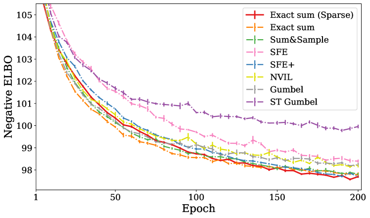
Method	Accuracy (%)	Dec. calls
Monte Carlo
SFE	$94.75$$\pm.002$	$1$
SFE$+$	$96.53$$\pm.001$	$2$
NVIL	$96.01$$\pm.002$	$1$
Sum&Sample	$96.73$$\pm.001$	$2$
Gumbel	$95.46$$\pm.001$	$1$
ST Gumbel	$86.35$$\pm.006$	$1$
Marginalization
Dense	$96.93$$\pm.001$	$10$
Sparse (proposed)	$96.87$$\pm.001$	$1.01$$\pm 0.01$

Figure 1: Semisupervised VAE on MNIST. Left: Learning curves (test). Right: Average test results and standard errors over 10 runs.

We consider the semisupervised VAE of Kingma et al. [29], which models the joint probability $p(z,h,x|\phi)=p(z)p(h)p(x|z,h)$, where $x$ is an observation (an MNIST image), $h$ is a continuous latent variable with a $n$-dimensional standard Gaussian prior, and $z$ is a discrete random variable with a uniform prior over $K$ categories. The marginal $p(x|\phi)=\sum_{z=1}^{K}\int_{h}p(x|z,h,\phi)p(h)p(z)\operatorname{d}\!h$ is intractable, due to the marginalization of $h\in\mathbb{R}^{n}$. For a fixed $h$ (e. g., sampled), marginalizing $z$ requires $K$ calls to the decoder, which can be costly depending on the decoder’s architecture.

To circumvent the need for the marginal likelihood, Kingma et al. [29] use variational inference [30] with an approximate posterior $\pi(z|x,\theta_{\pi})q(h|z,x,\lambda)$. This trains a classifier $\pi(z|x,\theta_{\pi})$ along with the generative model. In [29], $h$ is sampled with a reparameterization, and the expectation over $z$ is computed in closed-form, that is, assessing all $K$ terms of the sum for a sampled $h$. Under the notation in §2, we let $\theta_{\ell}=\{\lambda,\phi\}$ and define

$$\ell(x,z;\theta_{\ell})\coloneqq-\mathbb{E}_{q(h|z,\lambda)}\left[\operatorname*{\mathsf{log}}p(x\mid z,h,\phi)\right]-\operatorname*{\mathsf{log}}\frac{p(z)}{\pi(z\mid x,\theta_{\pi})}+\operatorname{\mathsf{KL}}\left[q(h\mid x,z,\lambda)\,\,\|\,\,p(h)\right],$$ (5)

which turns Eq. 1 into the (negative) evidence lower bound (ELBO). To update $q(h|x,z,\lambda)$, we use the reparameterization trick to obtain gradients through a sampled $h$. For $\pi(z|x,\theta_{\pi})$, we may still explicitly marginalize over each possible assignment of $z$, but this has a multiplicative cost on $K$. As an alternative, we parameterize $\pi(z|x,\theta_{\pi})$ with a sparse mapping, comparing it to the original formulation and with stochastic gradients based on SFE and continuous relaxations of $z$.

Data and architecture.

We evaluate this model on the MNIST dataset [31], using 10% of labeled data, treating the remaining data as unlabeled. For the parameterization of the model components we follow the architecture and training procedure used in [22]. Each model was trained for 200 epochs.

Comparisons.

Our proposal’s key ingredient is sparsity, which permits exact marginalization and a deterministic gradient. To investigate the impact of sparsity alone, we report a comparison against the exact marginalization over the entire support $\mathcal{Z}$ using a dense softmax parameterization. To investigate the impact of deterministic gradients, we compare to stochastic gradients. Unbiased gradient estimators: (i) SFE with a moving average baseline; (ii) SFE with a self-critic baseline [SFE+; 32], that is, we use $\operatorname*{\mathsf{log}}p(x|z^{\prime},h,\phi)$ as baseline, where $z^{\prime}\sim\pi(z|x,\theta_{\pi})$ is an independent sample; (iii) NVIL [33] with a learned baseline (we train a MLP to predict the learning signal by minimizing mean squared error); and (iv) sum-and-sample, a Rao-Blackwellized version of SFE [22]. Biased gradient estimators: (v) Gumbel-Softmax, which relaxes the random variable to the simplex, and (vi) ST Gumbel-Softmax, which discretizes the relaxation in the forward pass, but ignores the discretization function in the backward pass.

Results and discussion.

In Fig. 1, we see that our proposed sparse marginalization approach performs just as well as its dense counterpart, both in terms of ELBO and accuracy. However, by inspecting the number of times each method calls the decoder for assessments of $p(x|z,h,\phi)$, we can see that the effective support of our method is much smaller — sparsemax-parameterized posteriors get very confident, and mostly require one, and sometimes two, calls to the decoder. Regarding the Monte Carlo methods, the continuous relaxation done by Gumbel-Softmax underperformed all the other methods, with the exception of SFE with a moving average. While SFE+ and Sum&Sample are very strong performers, they will always require throughout training the same number of calls to the decoder (in this case, two). On the other hand, sparsemax makes a small number of decoder calls not due to a choice in hyperparameters but thanks to the model converging to only using a small support, which can endow this method with a lower number of computations as it becomes more confident.

5.2 Emergent Communication Game

Emergent communication studies how two agents can develop a communication protocol to solve a task collaboratively [34]. Recent work used neural latent variable models to train these agents via a “collaborative game” between them [35, 36, 37, 38, 39, 40]. In [36], one of the agents (the sender) sees an image $v_{y}$ and sends a single symbol message $z$ chosen from a set $\mathcal{Z}$ (the vocabulary) to the other agent (the receiver), who needs to choose the correct image $v_{y}$ out of a collection of images $\mathcal{V}=\left\{v_{1},\dots,v_{C}\right\}$. They found that the messages communicated this way can be correlated with broad object properties amenable to interpretation by humans. In our framework, we let $x=(\mathcal{V},y)$ and define $\ell(x,z;\theta)\coloneqq-\operatorname*{\mathsf{log}}p(y\mid\mathcal{V},z,\theta_{\ell})$ and $\pi(z\mid x,\theta)\coloneqq p(z\mid v_{y},\theta_{\pi})$, where $p(y\mid\mathcal{V},z,\theta_{\ell})$ corresponds to the sender and $p(z\mid v_{y},\theta_{\pi})$ to the receiver. Following Lazaridou et al. [36], we add an entropy regularization of $\pi(z\mid x,\theta)$ to the loss, with a coefficient as an hyperparameter [41].

Data and architecture.

We follow the architecture described in [36]. However, to make the game harder, we increase the collection of images $|\mathcal{V}|$ as suggested by [37]; in our experiments, we increase it from 2 to 16. All methods are trained for 500 epochs.

Comparisons.

We compare our method to stochastic gradient estimators as well as exact marginalization under a dense softmax parameterization of $p(z\mid v_{y},\theta_{\pi})$. Again, we have unbiased (SFE with moving average baseline, SFE+, and NVIL) and biased (Gumbel-Softmax and ST Gumbel-Softmax) estimators. For SFE we also experiment with a 0/1 loss, rather than negative log-likelihood (NLL).

Table 1: Emergent communication success test results, averaged across 10 runs. Random guess baseline $6.25\%$.

Method	Comm. succ. (%)		Dec. calls
Monte Carlo
SFE (NLL)	$33.05$	$\pm 2.84$	$1$
SFE (0/1)	$55.36$	$\pm 2.92$	$1$
SFE$+$ (0/1)	$44.32$	$\pm 2.72$	$2$
NVIL	$37.04$	$\pm 1.61$	$1$
Gumbel	$23.51$	$\pm 16.19$	$1$
ST Gumbel	$27.42$	$\pm 13.36$	$1$
Marginalization
Dense	$93.37$	$\pm 0.42$	$256$
Sparse (proposed)	$93.35$	$\pm 0.50$	$3.13$$\pm 0.48$

Results and discussion.

Table 1 shows the communication success (accuracy of the receiver at picking the correct image $v_{y}$). While the communication success for $|\mathcal{V}|=2$ in [36] was close to perfect, we see that increasing $|\mathcal{V}|$ to 16 makes this game much harder to sampling-based approaches. In fact, only the models that do explicit marginalization achieve close to perfect communication in the test set. However, as $\mathcal{Z}$ increases, marginalizing with a softmax parameterization gets computationally more expensive, as it requires $|\mathcal{Z}|$ forward and backward passes on the receiver. Unlike softmax, the model trained with sparsemax gives a very small support, requiring on average only 3 decoder calls. In fact, sparsemax starts off dense while exploring, but quickly becomes very sparse (App. F).

5.3 Bit-Vector Variational Autoencoder

As described in §4, in many interesting problems, combinatorial interactions and constraints make $\mathcal{Z}$ exponentially large. In this section, we study the illustrative case of encoding (compressing) images into a binary codeword $z$, by training a latent bit-vector variational autoencoder [11, 33]. One approach for parameterizing the approximate posterior is to use a Gibbs distribution, decomposable as a product of independent Bernoulli, $q(z\mid x,\lambda)\propto\operatorname*{\mathsf{exp}}(\langle\bm{a}_{z},\bm{t}\rangle)=\prod_{i=1}^{D}q(z_{i}\mid x,\lambda)$, with each $z_{i}$ being a Bernoulli with parameter $t_{i}$, and $D$ being the number of binary latent variables. While marginalizing over all the possible $z\in\mathcal{Z}$ is intractable, drawing samples can be done efficiently by sampling each component independently, and the entropy has a closed-form expression. This efficient sampling and entropy computation relies on an independence assumption; in general, we may not have access to such efficient computation.

Training this VAE to minimize the negative ELBO corresponds to $\ell(x,z;\theta_{\ell})\coloneqq-\operatorname*{\mathsf{log}}\frac{p(x,z|\phi)}{q(z|x,\lambda)}$; we use a uniform prior $p(z)=1/|\mathcal{Z}|=1/{2^{D}}$. This objective does not constrain $\pi(z|x,\theta_{\pi})\coloneqq q(z\mid x,\lambda)$ to the Gibbs parameterization, and thus to apply our methods we will differ from it.

Top-$k$ sparsemax parameterization.

As pointed out in §4, we cannot explicitly handle the structured sparsemax distribution $\bm{\xi}=\operatorname*{\mathsf{sparsemax}}(\bm{s})$, as it involves a vector of dimension $2^{D}$. However, given $\bm{t}$, we can efficiently find the $k$ largest configurations in time $\mathcal{O}(kD)$, with the procedure described in §4.1, and thus we can evaluate $\operatorname{\mathsf{sparsemax}_{\text{$k$}}}(\bm{s})$ efficiently.

SparseMAP parameterization.

Another sparse alternative to the intractable structured sparsemax, as discussed in §4, is SparseMAP. In this case, we compute an optimal distribution $\bm{\xi}$ using the active set algorithm of [13], by using a maximization oracle which can be computed in $\mathcal{O}(D)$:

$$\operatorname*{\mathsf{argmax}}_{z}\langle\bm{a}_{z},\bm{t}\rangle=z^{\star}\quad\text{s.t.}\quad[\bm{a}_{z^{\star}}]_{i}=\begin{cases}1,&t_{i}\geq 0\\ 0,&t_{i}<0\\ \end{cases}.$$ (6)

Since SparseMAP can handle structured problems, we also experimented with adding a budget constraint to SparseMAP: this is done by adding a constraint $\|\bm{z}\|_{1}\leq B$, where $B\leq D$; we used $b=\frac{D}{2}$. The budget constraint ensures the images are represented with sparse codes, and the maximization oracle can be computed in $\mathcal{O}(D\operatorname*{\mathsf{log}}D)$ as described in App. C.

We stress that, with both top-$k$ sparsemax and SparseMAP parameterizations, $z$ does not decompose into a product of independent binary variables: this property is specific to the Gibbs parameterization. However, since these new approaches induce a very sparse approximate posterior $q$, we may compute the terms $\mathbb{E}_{q(z\mid x,\lambda)}[\operatorname*{\mathsf{log}}p(x\mid z,\phi)]$ and $\mathbb{E}_{q(z\mid x,\lambda)}[\operatorname*{\mathsf{log}}q(z\mid x,\lambda)]$ explicitly.

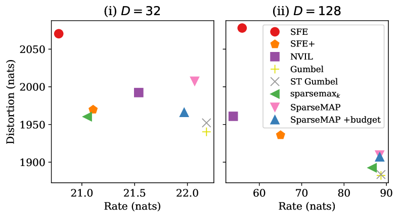
Method	$D=32$	$D=128$
Monte Carlo
SFE	$3.74$	$3.77$
SFE$+$	$3.61$	$3.59$
NVIL	$3.65$	$3.60$
Gumbel	$3.57$	$3.49$
ST Gumbel	$3.53$	$3.55$
Marginalization
Top-$k$ sparsemax	$3.62$	$3.61$
SparseMAP	$3.72$	$3.67$
SparseMAP (w/ budget)	$3.64$	$3.66$

Figure 2: Test results for Fashion-MNIST. Left and middle: RD plots (the closer to the lower right corner, the better). Right: NLL in bits/dim (lower, the better).

Data and architecture.

We use Fashion-MNIST [42], consisting of 256-level grayscale images $x\in{\{0,1,\dots,255\}}^{28\times 28}$. The decoder uses an independent categorical distribution for each pixel, $p(x\mid z,\phi)=\prod_{i=1}^{28}\prod_{j=1}^{28}p(x_{ij}\mid z,\phi)$. For top-$k$ sparsemax, we choose $k=10$.

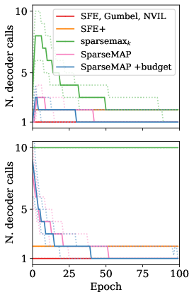
Figure 3: Bit vector VAE median and quartile decoder calls per epoch, $D=32$ (top) / $D=128$ (bottom).

Comparisons.

This time, exact marginalization under a dense parameterization of $q(z|x,\lambda)$ is truly intractable, so we can only compare our method to stochastic gradient estimators. We have unbiased SFE-based estimators (SFE with moving average baseline, SFE+, and NVIL), and biased reparameterized gradient estimators (Gumbel-Softmax and ST Gumbel-Softmax). As there is no supervision for the latent code, we cannot compare the methods in terms of accuracy or task success. Instead, we display the trained models in the rate-distortion (RD) plane [43] and also report bits-per-dimension of $x$, estimated with importance sampling (App. D), on held-out data.

Results and discussion.

Fig. 2 shows an importance sampling estimate ($1024$ samples per test example were taken) of the negative log-likelihood for the several methods, together with the converged values of each method in the RD plane. Both show results for which the bit-vector has dimensionality $D=32$ and $D=128$. Regarding the estimated negative log-likelihood, our methods exhibit increased performance when compared to SFE, and top-$k$ sparsemax is competitive with the remaining unbiased estimators. However, in the RD plane, both our methods show comparable performance to SFE$+$ and NVIL for $D=32$, but for $D=128$ all of our methods have a significantly higher rate and lower distortion than any unbiased estimator, suggesting a better fit of $p(x|\phi)$ [43]. In Fig. 3, we can observe the training progress in number of calls to $p(x\mid z,\phi)$ for the models with 32 and 128 latent bits, respectively. While $\operatorname{\mathsf{sparsemax}_{\text{$k$}}}$ introduces bias towards the most probable assignments and may discard outcomes that $\operatorname*{\mathsf{sparsemax}}$ would assign non-zero probability to, as training progresses distributions may (or tend to) be sufficiently sparse and this mismatch disappears, making the gradient computation exact. Remarkably, this happens for $D=32$ — the support of $\operatorname{\mathsf{sparsemax}_{\text{$k$}}}$ is smaller than $k$, giving the true gradient to $q(z\mid x,\lambda)$ for most of the training. This no longer happens for $D=128$, for which it remains with full support throughout, due to the much larger search space. On the other hand, SparseMAP solutions become very sparse from the start in both cases, while still obtaining good performance. There is, therefore, a trade-off between the solutions we propose: on one hand, $\operatorname{\mathsf{sparsemax}_{\text{$k$}}}$ can become exact with respect to the expectation in Eq. 1, but it only does so if the chosen $k$ is suitable to the difficulty of the model; on the other hand, SparseMAP may not offer an exact gradient to $q(z\mid x,\lambda)$, but its performance is very close to $\operatorname{\mathsf{sparsemax}_{\text{$k$}}}$ and its higher propensity for sparsity gifts it with less computation (App. F).

Concerning relaxed estimators, note that the reconstruction loss is computed given a continuous sample, rather than a discrete one, allowing it more flexibility to directly reduce distortion and potentially explaining why it does well in that regard. Moreover, the rate of the relaxed model is unknown, and instead we plot the rate as if $z$ was given discrete treatment, which, although common practice, makes comparisons to other estimators inadequate. For ST Gumbel-Softmax the situation is different since, after training, $z$ is given discrete treatment throughout. Its success shows that, unlike in the other tasks considered, training on biased gradients is not too problematic.

6 Related Work

Differentiable sparse mappings.

There has been recent interest in applying sparse mappings of discrete distributions in deep discriminative models [12, 13, 44, 45, 28], attention mechanisms [46, 47, 48, 49], and in topic models [50]. Our work focuses on the parameterization of distributions over latent variables with sparse mappings, on the computational advantage to be gained by sparsity, and on the contrast between our novel training method and common sampling-based methods.

Reducing sampling noise.

The sampling procedure found in SFE is a great source of variance in models that build upon this method. To reduce this variance, many works have proposed baselines [15, 16, 17]. VIMCO [51] is a multi-sample estimator which exploits variance reduction via input-dependent baselines as well as a lower bound on marginal likelihood which is tighter than the ELBO [52]. The number of samples in VIMCO is a hyperparameter that stays fixed throughout training. Our methods, in contrast, may take several decoder calls initially, but that number automatically decreases over time as training progresses. While baselines must be independent of the sample for which we assess the score function, exploiting correlation in the downstream losses of dependent samples holds potential for further variance reduction. These are known as control variates [53]. REBAR [18] exploits a continuous relaxation to obtain a dependent sample and uses the downstream loss assessed at the relaxed sample to define a control variate. RELAX [19], instead, learns to predict the downstream loss of the relaxed sample with an auxiliary network. In contrast, sparse marginalization works for any factorization where a primitive for $1$-best (or $k$-best) enumeration is available, and takes no additional parameters nor additional optimization objectives. Another line of work approximates argmax gradients by perturbed finite differences [54, 55]; this requires the same computation primitive as our approach, but is always biased. ARM [56] is a control variate based on antithetic samples [57]: it does not require relaxation nor additional parameters, but it only applies to factorial Bernoulli distributions. Closest to our work are variance reduction techniques that rely on partial marginalization, typically of the top-$k$ assignments to the latent variable [22, 58]. These methods show improved performance and variance reduction, but require rejection sampling, which can be challenging in structured problems.

7 Conclusion

We described a novel training strategy for discrete latent variable models, eschewing the common approach based on MC gradient estimation in favor of deterministic, exact marginalization under a sparse distribution. Sparsity leads to a powerful adaptive method, which can investigate fewer or more latent assignments $z$ depending on the ambiguity of a training instance $x$, as well as on the stage in training. We showcase the performance and flexibility of our method by investigating a variety of applications, with both discrete and structured latent variables, with positive results. Our models very quickly approach a small number of latent assignment evaluations per sample, but make progress much faster and overall lead to superior results. Our proposed method thus offer the accuracy and robustness of exact marginalization while meeting the efficiency and flexibility of score function estimator methods, providing a promising alternative.

Broader Impact

We discuss here the broader impact of our work. Discussion in this section is predominantly speculative, as the methods described in this work are not yet tested in broader applications. However, we do think that the methods described here can be applied to many applications — as this work is applicable to any model that contains discrete latent variables, even of combinatorial type.

Currently, the solutions available to train discrete latent variable models (LVMs) greatly rely on MC sampling, which can have high variance. Methods that aim to decrease this variance are often not trivial to train and to implement and may disincentivize practitioners from using this class of models. However, we believe that discrete LVMs have, in many cases, more interpretable and intuitive latent representations. Our methods offer: a simple approach in implementation to train these models; no addition in the number of parameters; low increase in computational overhead (especially when compared to more sophisticated methods of variance reduction [22]); and improved performance. Our code has been open-sourced as to ensure it’s scrutinizable by anyone and to boost any related future work that other researchers might want to pursue.

As we have already pointed out, oftentimes LVMs have superior explanatory power and so can aid in understanding cases in which the model failed the downstream task. Interpretability of deep neural models can be essential to better discover any ethically harmful biases that exist in the data or in the model itself.

On the other hand, the generative models discussed in this work may also pave the way for malicious use cases, such as is the case with Deepfakes, fake human avatars used by malevolent Twitter users, and automatically generated fraudulent news. Generative models are remarkable at sampling new instances of fake data and, with the power of latent variables, the interpretability discussed before can be used maliciously to further push harmful biases instead of removing them. Furthermore, our work is promising in improving the performance of LVMs with several discrete variables, that can be trained as attributes to control the sample generation. Attributes that can be activated or deactivated at will to generate fake data can both help beneficial and malignant users to finely control the generated sample. Our work may be currently agnostic to this, but we recognize the dangers and dedicate effort to combating any malicious applications.

Energy-wise, LVMs often require less data and computation than other models that rely on a massive amount of data and infrastructure. This makes LVMs ideal for situations where data is scarce, or where there are few computational resources to train large models. We believe that better latent variable modeling is a step forward in the direction of alleviating environmental concerns of deep learning research [59]. However, the models proposed in this work tend to use more resources earlier on in training than standard methods, and even though in the applications shown they consume much less as training progresses, it’s not clear if that trend is still observed in all potential applications.

In data science, LVMs, such as mixed-membership models [60], can be used to uncover correlations in large amounts of data, for example, by clustering observations. Training these models requires various degrees of approximations which are not without consequence, they may impact the quality of our conclusions and their fealty to the data. For example, variational inference tends to under-estimate uncertainty and give very little support to certain less-represented groups of variables. Where such a model informs decision-makers on matters that affect lives, these decisions may be based on an incomplete view of the correlations in the data and/or these correlations may be exaggerated in harmful ways. On the one hand, our work contributes to more stable training of LVMs, and thus it is a step towards addressing some of the many approximations that can blur the picture. On the other hand, sparsity may exhibit a larger risk of disregarding certain correlations or groups of observations, and thus contribute to misinforming the data scientist. At this point it is unclear to which extent the latter happens and, if it does, whether it is consistent across LVMs and their various uses. We aim to study this issue further and work with practitioners to identify failure cases.

Appendix A Computing sparsemax: Forward and Backward Passes

The sparsemax mapping [12], as discussed in Section 3, is given by the unique solution to

$$\operatorname*{\mathsf{sparsemax}}(\bm{s})\coloneqq\operatorname*{\mathsf{argmin}}_{\bm{\xi}\in\triangle^{K}}\|\bm{\xi}-\bm{s}\|_{2}^{2}\,.$$ (7)

As a projection onto a polytope, the solution is likely to fall on the boundaries or the corners of the set. In this case, points on the boundary of $\triangle^{K}$ have one or more zero coordinates. In contrast, $\operatorname*{\mathsf{softmax}}(\bm{s})\propto\operatorname*{\mathsf{exp}}(\bm{s})$ is always strictly inside the simplex. From the optimality conditions of the sparsemax problem (7), it follows that the solution must have the form:

$$\operatorname*{\mathsf{sparsemax}}(\bm{s})=\operatorname*{\mathsf{max}}(\bm{s}-\tau,0)\,,$$ (8)

where the maximum is elementwise, and $\tau$ is the unique value that ensures the result sums to one. Letting $\bar{\mathcal{Z}}$ be the set of nonzero coordinates in the solution, the normalization condition is equivalently

$$\tau=\frac{\sum_{z\in\bar{\mathcal{Z}}}s_{z}}{|\bar{\mathcal{Z}}|}\,.$$ (9)

Observing that small changes to $\bm{s}$ almost always have no effect on the support $\bar{\mathcal{Z}}$, differentiating Equation 8 gives

$$\frac{\partial\bar{\bm{\xi}}}{\partial\bar{\bm{s}}}=\bm{I}_{|\bar{\mathcal{Z}}|}-\frac{1}{|\bar{\mathcal{Z}}|}\bm{11}^{\top}\,,$$ (10)

where $\bar{\bm{\xi}}$ and ${\bar{\bm{s}}}$ denote the subsets of the respective vectors indexed by the support $\bar{\mathcal{Z}}$. Outside of the support, the partial derivatives are zero. (Cf. the more general result in [45, Proposition 2].) In terms of computation, $\tau$ may be found numerically using root finding algorithms on $f(\tau)=\operatorname*{\mathsf{max}}(\bm{s}-\tau,0)-1$. Alternatively, observe that it is enough to find $\bar{\mathcal{Z}}$. By showing that sparsemax must preserve the ordering, i. e., that if $s_{z^{\prime}}>s_{z}$ and $z\in\bar{\mathcal{Z}}$ then $z^{\prime}\in\bar{\mathcal{Z}}$, it can be shown that $\bar{\mathcal{Z}}$ must consist of the $k$ highest-scoring coordinates of $\bm{s}$, where $k$ can be find by inspection after sorting $\bm{s}$. This leads to a straightforward $\mathcal{O}(K\operatorname*{\mathsf{log}}K)$ algorithm due to Held [23, pp. 16–17]. This can be further pushed to $\mathcal{O}(K)$ using median pivoting algorithms [61]. We use a simpler implementation based on repeatedly calling $\operatorname{\mathsf{top}_{\text{$k$}}}$, doubling $k$ until the optimal solution is found. Since solutions get sparser over time and $\operatorname{\mathsf{top}_{\text{$k$}}}$ is GPU-accelerated in modern libraries [62], this strategy is very fast in practice.

Appendix B Computing SparseMAP: The Active Set Algorithm

In this section, we present the active set method [63, Chapters 16.4 & 16.5] as applied to the SparseMAP optimization problem (Eq. 4) [13]. This form of the algorithm, due to Martins et al. [64, Section 6], is a small variation of the formulation of Nocedal and Wright for handling the equality constraint. Recall the SparseMAP problem,

$$\operatorname*{\mathsf{argmin}}_{\bm{\xi}\in\triangle^{|\mathcal{Z}|}}\|\bm{A}\bm{\xi}-\bm{t}\|_{2}^{2}\,.$$ (11)

Assume that we could identify the support, or active set of an optimal solution $\bm{\xi}^{\star}$, denoted

$$\bar{\mathcal{Z}}\coloneqq\left\{z\in\mathcal{Z}\mid\xi^{\star}_{z}>0\right\}\,.$$

Then, given this set, we could find the solution to (11) by solving the lower-dimensional equality-constrained problem

$$\operatorname*{\mathsf{minimize}}\|\bar{\bm{A}}\bar{\bm{\xi}}-\bm{t}\|^{2}\quad\operatorname*{\mathsf{s.t.}}\quad\bm{1}^{\top}\bar{\bm{\xi}}=1\,,$$ (12)

where we denote by $\bar{\bm{A}}$ and $\bar{\bm{\xi}}$ the restrictions of $\bm{A}$ and $\bm{\xi}$ to the active set of structures $\bar{\mathcal{Z}}$. The solution to this equality-constrained QP satisfies the KKT optimality conditions,

$$\begin{bmatrix}{\bar{\bm{A}}}^{\top}\bar{\bm{A}}&\bm{1}\\ \bm{1}^{\top}&0\\ \end{bmatrix}\begin{bmatrix}\bar{\bm{\xi}}\\ \tau\end{bmatrix}=\begin{bmatrix}\bar{\bm{A}}^{\top}\bm{t}\\ 1\end{bmatrix}.$$ (13)

Of course, the optimal support is not known ahead of time. The active set algorithm attempts to guess the support in a greedy fashion, at each iteration either [if the solution of (13) is not feasible for (11)] dropping a structure from $\bar{\mathcal{Z}}$, or [otherwise] adding a new structure. Since the support changes one structure at a time, the design matrix in (13) gains or loses one row and column, so we may efficiently maintain its Cholesky decomposition via rank-one updates.

We now give more details about the computation. Denote the solution of Eq. 13, (extended with zeroes), by $\hat{\bm{\xi}}\in\triangle^{|\mathcal{Z}|}$. Since we might not have the optimal $\bar{\mathcal{Z}}$ yet, $\hat{\bm{\xi}}$ can be infeasible (some coordinates may be negative.) To account for this, we take a partial step in its direction,

$$\bm{\xi}^{(i+1)}=(1-\gamma)\bm{\xi}^{(i)}+\gamma\hat{\bm{\xi}}^{(i+1)}\,$$ (14)

where, to ensure feasibility, the step size is given by

$$\gamma=\operatorname*{\mathsf{min}}\left(1,\operatorname*{\mathsf{min}}_{z\in\bar{\mathcal{Z}};\xi^{(i)}_{z}>\hat{\xi}_{z}}\frac{\xi^{(i)}_{z}}{\xi^{(i)}_{z}-\hat{\xi}_{z}}\right)\,.$$ (15)

If, on the other hand, $\hat{\bm{\xi}}$ is feasible for (11), (so $\gamma=1$), we check whether we have a globally optimal solution. By construction, $\hat{\bm{\xi}}$ satisfies all KKT conditions except perhaps dual feasibility $\bm{\nu}\geq 0$, where $\nu_{z}$ is the dual variable (Lagrange multiplier) corresponding to the constraint $\xi_{z}\geq 0$. Denote $\bm{\mu}^{(i)}\coloneqq\bm{A}\bm{\xi}^{(i)}=\bar{\bm{A}}\bar{\bm{\xi}}^{(i)}$. For any $z\not\in\bar{\mathcal{Z}}$, the corresponding dual variable must satisfy

$$\nu_{z}=\tau^{(i)}-\langle\bm{a}_{z},\bm{t}-\bm{\mu}^{(i)}\rangle\,.$$ (16)

If the smallest dual variable is positive, then our current guess satisfies all optimality conditions. To find the smallest dual variable we can equivalently solve $\operatorname*{\mathsf{argmax}}_{z\in\mathcal{Z}}\langle\bm{a}_{z},\bm{t}-\bm{\mu}^{(i)}\rangle$, which is a maximization (MAP) oracle call. If the resulting $\nu_{z}$ is negative, then $z$ is the index of the most violated constraint $\xi_{z}\geq 0$; it is thus a good choice of structure to add to the active set.

The full procedure is given in Algorithm 1. The backward pass can be computed by implicit differentiation of the KKT system (13) w. r. t. $\bm{t}$, giving, as in [13],

$$\frac{\partial\bar{\bm{\xi}}}{\partial\bm{t}}=\bar{\bm{A}}\big{(}\bm{S}-\bm{ss}^{\top}/s\big{)},\quad\text{where}\quad\bm{S}=(\bar{\bm{A}}^{\top}\bar{\bm{A}})^{-1},\bm{s}=\bm{S1},s=\bm{1}^{\top}\bm{S1}\,.$$ (17)

It is possible to apply the $\ell_{2}$ regularization term only to a subset of the rows of $\bm{A}$, as is more standard in the graphical model literature. We refer the reader to the presentation in [64, 13] for this extension.

Algorithm 1 Active set algorithm for SparseMAP

1:Init: $\bar{\mathcal{Z}}^{(0)}=\{z^{(0)}\}$  where  $z^{(0)}\in\operatorname*{\mathsf{argmax}}_{z\in\mathcal{Z}}\langle\bm{a}_{z},\bm{t}\rangle$ or a random structure.

2:for i in $1,\ldots,N$ do

3:    Compute $\tau^{(i)}$ and $\hat{\bm{\xi}}^{(i)}$ by solving the relaxed QP (Eq. 13). $\triangleright$ Cholesky update.

4:    $\bm{\xi}^{(i)}\leftarrow(1-\gamma)\bm{\xi}^{(i-1)}+\gamma\hat{\bm{\xi}}^{(i)}$  (with $\gamma$ from Eq. 15).

5:    if $\gamma<1$ then

6:         Drop the minimizer of Eq. 15 from $\bar{\mathcal{Z}}^{(i)}$.

7:    else

8:         Find most violated constraint, $z^{(i)}\leftarrow\operatorname*{\mathsf{argmin}}_{z\in\mathcal{Z}}\nu_{z}$. $\triangleright$ Eq. 16, MAP oracle.

9:         if $\nu_{z^{(i)}}\geq 0$ then

10:             return $\triangleright$ Converged.

11:         else

12:             $\mathcal{Z}^{(i+1)}\leftarrow\mathcal{Z}^{(i)}\cup\{z^{(i)}\}$              

Appendix C Budget Constraint

The maximization oracle for the budget constraint described in §5.3 can be computed in $\mathcal{O}(D\operatorname*{\mathsf{log}}D)$. This is done by sorting the Bernoulli scores and selecting the entries among the top-$B$ which have a positive score.

Appendix D Importance Sampling of the Marginal Log-Likelihood

Bits-per-dimension is the negative logarithm of marginal likelihood normalized per number of pixels in the image, thus we need to assess or estimate the marginal likelihood of observations. For dense parameterizations, the usual option is importance sampling (IS) using the trained approximate posterior as importance distribution: i. e., $\operatorname*{\mathsf{log}}p(x|\phi)\overset{\text{IS}}{\approx}\operatorname*{\mathsf{log}}\left(\frac{1}{S}\sum_{s=1}^{S}\frac{p(z^{(s)},x|\phi)}{q(z^{(s)}|x,\lambda)}\right)$ with $z^{(s)}\sim q(z|x,\lambda)$. The result is a stochastic lower bound which converges to the true log-marginal in the limit as $S\to\infty$. With a sparse posterior approximation we can split the marginalization

$$\operatorname*{\mathsf{log}}p(x|\phi)=\operatorname*{\mathsf{log}}\left(\sum_{z\in\bar{\mathcal{Z}}}p(z)p(x|z,\phi)+\sum_{z\in\mathcal{Z}\setminus\mathcal{Z}}p(z)p(x|z,\phi)\right)$$ (18)

into one part that handles outcomes in the support $\bar{\mathcal{Z}}$ of the sparse posterior approximation and another part that handles the outcomes in the complement set $\mathcal{Z}\setminus\bar{\mathcal{Z}}$. We compute the first part exactly and estimate the second part via rejection sampling from $p(z)$.

Appendix E Training Details

In our applications, we follow the experimental procedures described in [22] and [36] for §5.1 and §5.2, respectively. We describe below the most relevant training details and key differences in architectures when applicable. For other implementation details that we do not mention here, we refer the reader to the works referenced above. For all Gumbel baselines, we relax the sample into the continuous space but assume a discrete distribution when computing the entropy of $\pi(z\mid x,\theta)$, as suggested as one implementation option in Maddison et al. [10]. Our code is publicly available at https://github.com/deep-spin/sparse-marginalization-lvm and was largely inspired by the structure and implementations found in EGG [65] and was built upon it.

Semisupervised Variational Autoencoder.

In this experiment, the classification network consists of three fully connected hidden layers of size 256, using ReLU activations. The generative and inference network both consist of one hidden layer of size 128, also with ReLU activations. The multivariate Gaussian has 8 dimensions and its covariance is diagonal. For all models we have chosen the learning rate based on the best ELBO on the validation set, doing a grid search (5e-5, 1e-4, 5e-4, 1e-3, 5e-3). The accuracy shown in Fig. 1 is the test accuracy taken after the last epoch of training. The temperature of the Gumbel models was annealed according to $\tau=\operatorname*{\mathsf{max}}\left(0.5,-rt\right)$, where $t$ is the global training step. For these models, we also did a grid search over $r$ (1e-5, 1e-4) and over the frequency of updating $\tau$ every (500, 1000) steps. Optimization was done with Adam. For our method, in the labeled loss component of the semisupervised objective we used the sparsemax loss [12]. Following Liu et al. [22], we pretrain the network with only labeled data prior to training with the whole training set. Likewise, for our method, we pretrained the network on the sparsemax loss and every other method with the Negative Log-Likelihood loss.

Emergent communication game.

In this application, we closely followed the experimental procedure described by Lazaridou et al. [36] with a few key differences. The architecture of the sender and the receiver is identical with the exception that the sender does not take as input the distracting images along with the correct image --- only the correct image. The collection of images shown to the receiver was increased from 2 to 16 and the vocabulary of the sender was increased to 256. The hidden size and embedding size was also increased to 512 and 256, respectively. We did a grid search on the learning rate (0.01, 0.005, 0.001) and entropy regularizer (0.1, 0.05, 0.01) and chose the best configuration for each model on the validation set based on the communication success. For the Gumbel models, we applied the same schedule and grid search to the temperature as described for Semisupervised VAE. All models were trained with the Adam optimizer, with a batch size of 64 and during 200 epochs. We choose the vocabulary of the sender to be 256, the hidden size to be 512 and the embedding size to be 256.

Bit-Vector Variational Autoencoder.

In this experiment, we have set the generative and inference network to consist of one hidden layer with 128 nodes, using ReLU activations. We have searched a learning rate doing grid search (0.0005, 0.001, 0.002) and chosen the model based on the ELBO performance on the validation set. For the Gumbel models, we applied the same schedule and grid search to the temperature as described for Semisupervised VAE. We used the Adam optimizer.

E.1 Datasets

Semisupervised Variational Autoencoder.

MNIST consists of $28\times 28$ gray-scale images of hand-written digits. It contains 60,000 datapoints for training and 10,000 datapoints for testing. We perform model selection on the last 10,000 datapoints of the training split.

Emergent communication game.

The data used by Lazaridou et al. [36] is a subset of ImageNet containing 463,000 images, chosen by sampling 100 images from 463 base-level concepts. The images are then applied a forward-pass through the pretrained VGG ConvNet [66] and the representations at the second-to-last fully connected layer are saved to use as input to the sender/receiver.

Bit-Vector Variational Autoencoder.

Fashion-MNIST consists of $28\times 28$ gray-scale images of clothes. It contains 60,000 datapoints for training and 10,000 datapoints for testing. We perform model selection on the last 10,000 datapoints of the training split.

Appendix F Performance in Decoder Calls

Fig. 4 shows the number of decoder calls with percentiles for the experiment in §5.2. While dense right at the beginning of training, support quickly falls to an average of close to $1$ decoder call.

Fig. 5 shows the downstream loss (ELBO) of experiment §5.3 over epochs and over the median number of decoder calls per epoch. The plots on Fig. 5(b) show how our methods have comparable computational overhead to sampling approaches. Oftentimes, our methods could have been trained in less epochs to obtain the same performance as the sampling estimators have for 100 epochs.

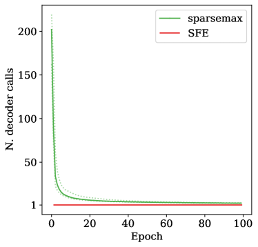
Figure 4: Median decoder calls per epoch during training time with 10 and 90 percentiles in dotted lines by sparsemax in §5.2.

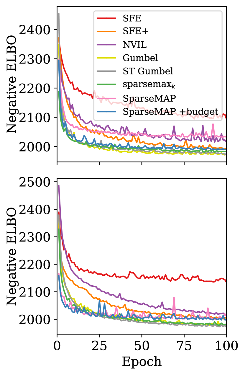
(a) Negative ELBO over training epochs.

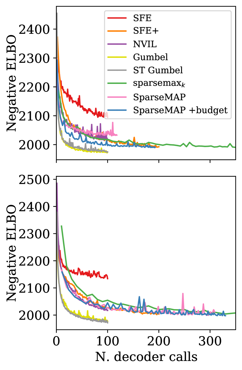
(b) Negative ELBO over decoder calls.

Figure 5: Performance on the validation set for the experiment in §5.3, $D=32$ (top) / $D=128$ (bottom). For $D=32$, top-$k$ sparsemax continues until a total of 561 median decoder calls, and for $D=128$ it continues until a total of 998.

Appendix G Computing infrastructure

Our infrastructure consists of 4 machines with the specifications shown in Table 2. The machines were used interchangeably, and all experiments were executed in a single GPU. Despite having machines with different specifications, we did not observe large differences in the execution time of our models across different machines.

#	GPU	CPU
1.	4 $\times$ Titan Xp - 12GB	16 $\times$ AMD Ryzen 1950X @ 3.40GHz - 128GB
2.	4 $\times$ GTX 1080 Ti - 12GB	8 $\times$ Intel i7-9800X @ 3.80GHz - 128GB
3.	3 $\times$ RTX 2080 Ti - 12GB	12 $\times$ AMD Ryzen 2920X @ 3.50GHz - 128GB
4.	3 $\times$ RTX 2080 Ti - 12GB	12 $\times$ AMD Ryzen 2920X @ 3.50GHz - 128GB

Table 2: Computing infrastructure.

References

- Kim et al. [2018] Yoon Kim, Sam Wiseman, and Alexander M. Rush. A tutorial on deep latent variable models of natural language. preprint arXiv:1812.06834, 2018.
- Kingma and Welling [2014] Diederik P. Kingma and Max Welling. Auto-encoding variational Bayes. In Proc. ICLR, 2014.
- Rezende et al. [2014] Danilo Jimenez Rezende, Shakir Mohamed, and Daan Wierstra. Stochastic backpropagation and approximate inference in deep generative models. In Proc. ICML, 2014.
- Titov and McDonald [2008] Ivan Titov and Ryan McDonald. A joint model of text and aspect ratings for sentiment summarization. In Proc. ACL, 2008.
- Bastings et al. [2019] Jasmijn Bastings, Wilker Aziz, and Ivan Titov. Interpretable neural predictions with differentiable binary variables. In Proc. ACL, 2019.
- Mohamed et al. [2019] Shakir Mohamed, Mihaela Rosca, Michael Figurnov, and Andriy Mnih. Monte Carlo gradient estimation in machine learning. preprint arXiv:1906.10652, 2019.
- Rubinstein [1976] RY Rubinstein. A Monte Carlo method for estimating the gradient in a stochastic network. Unpublished manuscript, Technion, Haifa, Israel, 1976.
- Paisley et al. [2012] John Paisley, David M. Blei, and Michael I. Jordan. Variational bayesian inference with stochastic search. In Proc. ICML, 2012.
- Bengio et al. [2013] Yoshua Bengio, Nicholas Léonard, and Aaron Courville. Estimating or propagating gradients through stochastic neurons for conditional computation. preprint arXiv:1308.3432, 2013.
- Maddison et al. [2017] Chris J. Maddison, Andriy Mnih, and Yee Whye Teh. The Concrete distribution: a continous relaxation of discrete random variables. In Proc. ICLR, 2017.
- Jang et al. [2017] Eric Jang, Shixiang Gu, and Ben Poole. Categorical reparameterization with Gumbel-Softmax. In Proc. ICLR, 2017.
- Martins and Astudillo [2016] André Martins and Ramon Astudillo. From softmax to sparsemax: a sparse model of attention and multi-label classification. In Proc. ICML, 2016.
- Niculae et al. [2018a] Vlad Niculae, André FT Martins, Mathieu Blondel, and Claire Cardie. SparseMAP: differentiable sparse structured inference. In Proc. ICML, 2018a.
- Robbins and Monro [1951] Herbert Robbins and Sutton Monro. A stochastic approximation method. The Annals of Mathematical Statistics, 22(3):400–407, 1951.
- Williams [1992] Ronald J. Williams. Simple statistical gradient-following algorithms for connectionist reinforcement learning. Machine Learning, 8(3-4):229–256, 1992.
- Gu et al. [2016] Shixiang Gu, Sergey Levine, Ilya Sutskever, and Andriy Mnih. MuProp: unbiased backpropagation for stochastic neural networks. In Proc. ICLR, 2016.
- Wang et al. [2013] Chong Wang, Xi Chen, Alexander J Smola, and Eric P Xing. Variance reduction for stochastic gradient optimization. In Proc. NeurIPS, 2013.
- Tucker et al. [2017] George Tucker, Andriy Mnih, Chris J Maddison, John Lawson, and Jascha Sohl-Dickstein. REBAR: low-variance, unbiased gradient estimates for discrete latent variable models. In Proc. NeurIPS, 2017.
- Grathwohl et al. [2018] Will Grathwohl, Dami Choi, Yuhuai Wu, Geoffrey Roeder, and David Duvenaud. Backpropagation through the void: optimizing control variates for black-box gradient estimation. In Proc. ICLR, 2018.
- Casella and Robert [1996] George Casella and Christian P Robert. Rao-Blackwellisation of sampling schemes. Biometrika, 83(1):81–94, 1996.
- Ranganath et al. [2014] Rajesh Ranganath, Sean Gerrish, and David Blei. Black box variational inference. In Proc. AISTATS, 2014.
- Liu et al. [2019] Runjing Liu, Jeffrey Regier, Nilesh Tripuraneni, Michael Jordan, and Jon Mcauliffe. Rao-Blackwellized stochastic gradients for discrete distributions. In Proc. ICML, 2019.
- Held et al. [1974] Michael Held, Philip Wolfe, and Harlan P Crowder. Validation of subgradient optimization. Mathematical Programming, 6(1):62–88, 1974.
- Wainwright and Jordan [2008] Martin J Wainwright and Michael I Jordan. Graphical models, exponential families, and variational inference. Foundations and Trends® in Machine Learning, 1(1-2):1–305, 2008.
- Kyrillidis et al. [2013] Anastasios Kyrillidis, Stephen Becker, Volkan Cevher, and Christoph Koch. Sparse projections onto the simplex. In Proc. ICML, 2013.
- Pillutla et al. [2018] Venkata Krishna Pillutla, Vincent Roulet, Sham M Kakade, and Zaid Harchaoui. A Smoother Way to Train Structured Prediction Models. In Proc. NeurIPS, 2018.
- Blondel et al. [2020] Mathieu Blondel, André F.T. Martins, and Vlad Niculae. Learning with Fenchel-Young losses. Journal of Machine Learning Research, 21(35):1–69, 2020.
- Niculae et al. [2018b] Vlad Niculae, André FT Martins, and Claire Cardie. Towards dynamic computation graphs via sparse latent structure. In Proc. EMNLP, 2018b.
- Kingma et al. [2014] Durk P Kingma, Shakir Mohamed, Danilo Jimenez Rezende, and Max Welling. Semi-supervised learning with deep generative models. In Proc. NeurIPS, 2014.
- Jordan et al. [1999] Michael I Jordan, Zoubin Ghahramani, Tommi S Jaakkola, and Lawrence K Saul. An introduction to variational methods for graphical models. Machine Learning, 37(2):183–233, 1999.
- LeCun et al. [1998] Yann LeCun, Léon Bottou, Yoshua Bengio, and Patrick Haffner. Gradient-based learning applied to document recognition. Proc. IEEE, 86(11):2278–2324, 1998.
- Rennie et al. [2017] Steven J Rennie, Etienne Marcheret, Youssef Mroueh, Jerret Ross, and Vaibhava Goel. Self-critical sequence training for image captioning. In Proc. CVPR, 2017.
- Mnih and Gregor [2014] Andriy Mnih and Karol Gregor. Neural variational inference and learning in belief networks. In Proc. ICML, 2014.
- Kirby [2002] Simon Kirby. Natural language from artificial life. Artificial life, 8(2):185–215, 2002.
- Lewis [1969] David Lewis. Convention: A philosophical study. 1969.
- Lazaridou et al. [2017] Angeliki Lazaridou, Alexander Peysakhovich, and Marco Baroni. Multi-agent cooperation and the emergence of (natural) language. In Proc. ICLR, 2017.
- Havrylov and Titov [2017] Serhii Havrylov and Ivan Titov. Emergence of language with multi-agent games: Learning to communicate with sequences of symbols. In Proc. NeurIPS, 2017.
- Jorge et al. [2016] Emilio Jorge, Mikael Kågebäck, Fredrik D. Johansson, and Emil Gustavsson. Learning to play guess who? and inventing a grounded language as a consequence. In Proc. NeurIPS Workshop on Deep Reinforcement Learning, 2016.
- Foerster et al. [2016] Jakob Foerster, Ioannis Alexandros Assael, Nando De Freitas, and Shimon Whiteson. Learning to communicate with deep multi-agent reinforcement learning. In Proc. NeurIPS, 2016.
- Sukhbaatar et al. [2016] Sainbayar Sukhbaatar, Arthur Szlam, and Rob Fergus. Learning Multiagent Communication with Backpropagation. In Proc. NeurIPS, 2016.
- Mnih et al. [2016] Volodymyr Mnih, Adria Puigdomenech Badia, Lehdi Mirza, Alex Graves, Tim Harley, Timothy P. Lillicrap, David Silver, and Koray Kavukcuoglu. Asynchronous Methods for Deep Reinforcement Learning. In Proc. ICML, 2016.
- Xiao et al. [2017] Han Xiao, Kashif Rasul, and Roland Vollgraf. Fashion-MNIST: a novel image dataset for benchmarking machine learning algorithms. preprint arXiv:1708.07747, 2017.
- Alemi et al. [2018] Alexander A. Alemi, Ben Poole, Ian Fischer, Joshua V. Dillon, Rif A. Saurous, and Kevin Murphy. Fixing a Broken ELBO. In Proc. ICML, 2018.
- Niculae and Blondel [2017] Vlad Niculae and Mathieu Blondel. A regularized framework for sparse and structured neural attention. In Proc. NeurIPS, 2017.
- Peters et al. [2019] Ben Peters, Vlad Niculae, and André FT Martins. Sparse sequence-to-sequence models. In Proc. ACL, 2019.
- Malaviya et al. [2018] Chaitanya Malaviya, Pedro Ferreira, and André FT Martins. Sparse and constrained attention for neural machine translation. In Proc. ACL, 2018.
- Shao et al. [2019] Wenqi Shao, Tianjian Meng, Jingyu Li, Ruimao Zhang, Yudian Li, Xiaogang Wang, and Ping Luo. SSN: Learning sparse switchable normalization via SparsestMax. In Proc. CVPR, 2019.
- Maruf et al. [2019] Sameen Maruf, André FT Martins, and Gholamreza Haffari. Selective attention for context-aware neural machine translation. In Proc. NAACL-HLT, 2019.
- Correia et al. [2019] Gonçalo M Correia, Vlad Niculae, and André FT Martins. Adaptively sparse transformers. In Proc. EMNLP, 2019.
- Cao [2019] Kris Cao. Learning Meaning Representations for Text Generation with Deep Generative Models. PhD thesis, University of Cambridge, 2019.
- Mnih and Rezende [2016] Andriy Mnih and Danilo J. Rezende. Variational inference for Monte Carlo objectives. In Proc. ICML, 2016.
- Burda et al. [2016] Yuri Burda, Roger B. Grosse, and Ruslan Salakhutdinov. Importance Weighted Autoencoders. In Proc. ICLR, 2016.
- Greensmith et al. [2004] Evan Greensmith, Peter L. Bartlett, and Jonathan Baxter. Variance Reduction Techniques for Gradient Estimates in Reinforcement Learning. JMLR, 5(Nov):1471–1530, 2004.
- Lorberbom et al. [2019] Guy Lorberbom, Andreea Gane, Tommi Jaakkola, and Tamir Hazan. Direct Optimization through for Discrete Variational Auto-Encoder. In Proc. NeurIPS, 2019.
- Vlastelica et al. [2020] Marin Vlastelica, Anselm Paulus, Vit Musil, Georg Martius, and Michal Rolinek. Differentiation of blackbox combinatorial solvers. In Proc. ICLR, 2020.
- Yin and Zhou [2019] Mingzhang Yin and Mingyuan Zhou. ARM: Augment-REINFORCE-Merge Gradient for Stochastic Binary Networks. In Proc. ICLR, 2019.
- Owen [2013] Art B. Owen. Monte Carlo theory, methods and examples. 2013.
- Kool et al. [2020] Wouter Kool, Herke van Hoof, and Max Welling. Estimating Gradients for Discrete Random Variables by Sampling without Replacement. In Proc. ICLR, 2020.
- Strubell et al. [2019] Emma Strubell, Ananya Ganesh, and Andrew McCallum. Energy and Policy Considerations for Deep Learning in NLP. In Proc. ACL, 2019.
- Blei [2014] David M Blei. Build, compute, critique, repeat: Data analysis with latent variable models. Annual Review of Statistics and Its Application, 1:203–232, 2014.
- Condat [2016] Laurent Condat. Fast projection onto the simplex and the ball. Mathematical Programming, 158(1-2):575–585, 2016.
- Paszke et al. [2019] Adam Paszke, Sam Gross, Francisco Massa, Adam Lerer, James Bradbury, Gregory Chanan, Trevor Killeen, Zeming Lin, Natalia Gimelshein, Luca Antiga, Alban Desmaison, Andreas Kopf, Edward Yang, Zachary DeVito, Martin Raison, Alykhan Tejani, Sasank Chilamkurthy, Benoit Steiner, Lu Fang, Junjie Bai, and Soumith Chintala. PyTorch: An Imperative Style, High-Performance Deep Learning Library. In Proc. NeurIPS, 2019.
- Nocedal and Wright [1999] Jorge Nocedal and Stephen Wright. Numerical Optimization. Springer New York, 1999.
- Martins et al. [2015] André FT Martins, Mário AT Figueiredo, Pedro MQ Aguiar, Noah A Smith, and Eric P Xing. AD3: Alternating directions dual decomposition for MAP inference in graphical models. JMLR, 16(1):495–545, 2015.
- Kharitonov et al. [2019] Eugene Kharitonov, Rahma Chaabouni, Diane Bouchacourt, and Marco Baroni. EGG: a toolkit for research on Emergence of lanGuage in Games. In Proc. EMNLP, 2019.
- Simonyan and Zisserman [2015] Karen Simonyan and Andrew Zisserman. Very deep convolutional networks for large-scale image recognition. In Proc. ICLR, 2015.