Universal Distances for Extended Persistence

Abstract

The extended persistence diagram is an invariant of piecewise linear functions, which is known to be stable under perturbations of functions with respect to the bottleneck distance as introduced by Cohen-Steiner, Edelsbrunner, and Harer. We address the question of universality, which asks for the largest possible stable distance on extended persistence diagrams, showing that a more discriminative variant of the bottleneck distance is universal. Our result applies more generally to settings where persistence diagrams are considered only up to a certain degree. We achieve our results by establishing a functorial construction and several characteristic properties of relative interlevel set homology, which mirror the classical Eilenberg–Steenrod axioms. Finally, we contrast the bottleneck distance with the interleaving distance of sheaves on the real line by showing that the latter is not intrinsic, let alone universal. This particular result has the further implication that the interleaving distance of Reeb graphs is not intrinsic either.

1 Introduction

The core idea of topological persistence is to construct invariants of continuous real-valued functions by considering preimages and applying homology with coefficients in a fixed field $K$, or any other functorial invariant from algebraic topology. The most basic incarnation of this idea studies the homology of sublevel sets. Sublevel set persistent homology was introduced in [ELZ02] and is described up to isomorphism by the sublevel set persistence diagram [CSEH07]. An extension of this invariant considers preimages of arbitrary intervals, where non-closed intervals are treated using relative homology [DW07, CdM09] This is commonly referred to as the Mayer–Vietoris pyramid, due to its connection to the relative Mayer–Vietoris sequence.

As shown by [CdM09], interlevel set persistent homology of a PL function $f\colon X\rightarrow\mathbb{R}$ on a finite connected simplicial complex, is described up to isomorphism by the extended persistence diagram $\operatorname{Dgm}(f)$ due to [CSEH09]. It is well-known that the operation ${f\mapsto\operatorname{Dgm}(f)}$ is stable [CSEH09, HKLM19], by an extension of the classical stability result for sublevel set persistence [CSEH07] to the setting of extended persistence. Specifically, for functions $f,g\colon X\to\mathbb{R}$ as above,

$$d_{B}(\operatorname{Dgm}(f),\operatorname{Dgm}(g))\leq||f-g||_{\infty},$$

where $d_{B}(\operatorname{Dgm}(f),\operatorname{Dgm}(g))$ is the bottleneck distance of $\operatorname{Dgm}(f)$ and $\operatorname{Dgm}(g)$.

In this paper we prove that this distance is universal: it is the largest possible stable distance on extended persistence diagrams realized by functions. As a note of caution, we point out that universality is only achieved by a version of the bottleneck distance in which any vertex contained inside the extended subdiagram has to be matched, as is made precise in Remark 2.5.

We obtain this universality result by exploring the structure behind extended persistence. As observed already in [CdM09], the connecting homomorphisms allow us to assemble the Mayer–Vietoris pyramids of all degrees into a single diagram, with the shape of an infinite strip. We denote this strip by $\mathbb{M}$, alluding to the fact that it can naturally be interpreted as the universal cover of a Möbius strip whose points correspond to pairs of preimages of $f$ whose relative homology we want to consider, and we refer to the strip-shaped diagram as the relative interlevel set homology of the function $f$ and denote it by $h(f)\colon\mathbb{M}\rightarrow\mathrm{Vect}_{K}$. The resulting diagram now consists of all relative homology groups of those pairs, separated by homological degrees, and with all possible maps induced by either inclusions or connecting homomorphisms. It is easily overlooked that establishing the commutativity of this strip-shaped diagram actually raises several technical challenges; in the present paper, we give a rigorous construction, extending the definitions from the previous literature to also make the gluing of the Mayer–Vietoris pyramids explicit in a functorial way.

We also define the associated extended persistence diagram $\operatorname{Dgm}(f)$ in terms of the functor $h(f)$ in Section 2.2 as a multiset on the interior of $\mathbb{M}$. Note that we write $\operatorname{int}\mathbb{M}$ to denote this interior of $\mathbb{M}$ as usual in topology, and not the intervals in $\mathbb{M}$, which often play a role in persistence theory too. While our definition turns out to be equivalent to the familiar one from [CSEH09], our approach is natural in the context of relative interlevel set persistence, clarifying the above mentioned conditions on matchings required to yield a universal bottleneck distance. In Appendix B we use a structure theorem for relative interlevel set homology to show that the ordinary, relative, and extended subdiagrams, as originally defined in [CSEH09], can be obtained by restriction to the corresponding regions depicted in Fig. 1.1.

Figure 1.1: Regions in the strip $\mathbb{M}$ corresponding to the ordinary, relative, and extended subdiagrams [CSEH09]. The support of extended persistence diagrams is shaded in grey.

In practice it may be undesirable or even intractable to compute the entire extended persistence diagram of $f\colon X\rightarrow\mathbb{R}$. Instead, it might be preferable to compute just the restriction of $\operatorname{Dgm}(f)\colon\operatorname{int}\mathbb{M}\rightarrow\mathbb{N}_{0}$ to some closed upset $\mathbb{U}\subseteq\mathbb{M}$. Now in order for the bottleneck distance of Definition 2.4 below to be universal, when applied to such restricted persistence diagrams, we need to impose some restrictions on the upset $\mathbb{U}\subseteq\mathbb{M}$ (arising from the fact that 4.6 below is invalid for arbitrary closed upsets $\mathbb{U}\subseteq\mathbb{M}$). In Fig. 1.1 the grey shaded region is triangulated by the solid and the dashed lines, with each triangle corresponding to a face of a Mayer–Viatoris pyramid. We say that a closed upset $\mathbb{U}\subseteq\mathbb{M}$ is admissible, if it contains the region labeled $\operatorname{Ext}_{0}$ and if it is compatible with this triangulation in the sense that the interior of each triangle is either fully contained in or disjoint from $\mathbb{U}$. Moreover, for an admissible upset $\mathbb{U}\subseteq\mathbb{M}$ we say that a multiset $\mu\colon\operatorname{int}\mathbb{U}\rightarrow\mathbb{N}_{0}$ is a realizable persistence diagram if $\mu=\operatorname{Dgm}(f)|_{\operatorname{int}\mathbb{U}}$ for some function $f$ as above. Roughly speaking, we may think of the restriction of $\operatorname{Dgm}(f)\colon\operatorname{int}\mathbb{M}\rightarrow\mathbb{N}_{0}$ to the interior of an admissble upset $\mathbb{U}\subset\mathbb{M}$ as the graded barcode truncated at some upper bound for the degree with respect to a certain kind of persistence. Using the terminology introduced by [CdM09], the five kinds of persistence that may occur for an admissible upset $\mathbb{U}\subset\mathbb{M}$ are levelset (zigzag), up-down, down-up, extended persistence, and extended persisence of $-f$. For extended persistence, $\mathbb{U}$ is the union of all regions corresponding to subdiagrams not exceeding a certain degree as depicted in Fig. 1.1. Universality now follows immediately from the following slightly stronger theorem.

Theorem 1.1.

For an admissible upset $\mathbb{U}$ and any two realizable persistence diagrams $\mu,\nu\colon\operatorname{int}\mathbb{U}\rightarrow\mathbb{N}_{0}$ with $d_{B}(\mu,\nu)<\infty$, there exists a finite simplicial complex $X$ and piecewise linear functions $f,g\colon X\rightarrow\mathbb{R}$ with

$$\operatorname{Dgm}(f)|_{\operatorname{int}\mathbb{U}}=\mu,\quad\operatorname{Dgm}(g)|_{\operatorname{int}\mathbb{U}}=\nu,~{}\text{and}\quad d_{B}(\mu,\nu)=\lVert f-g\rVert_{\infty}.$$

Since the stability inequality $d_{B}(\mu,\nu)\leq\lVert f-g\rVert_{\infty}$ is attained for all $\mu,\nu$, the bottleneck distance is universal. Note that this also immediately implies that the bottleneck distance is geodesic (and hence intrinsic), with an explicit geodesic between $\mu,\nu$ being given by the 1-parameter family of extended persistence diagrams of the convex combinations $(1-\lambda)f+\lambda g$ of $f$ and $g$; see also 4.7.

An analogous realizability theorem in the context of sublevel set persistent homology has already been given in [Les15], and special cases have been considered in several other works [DeS21, CCF⁺20, CCF⁺20]. Universality of metrics has further been studied for various other common constructions in topological data anaysis, such as Reeb graphs [BLM21], contour trees and merge trees [BBF22, CCLL22], and the general setting of locally persistent categories [Sco20]. We stress that the persistence diagrams considered here contain information about homology in any degree represented in $\mathbb{U}$.

It is worth noting that the realization of a pair of extended persistence diagrams is more intricate than the realization of a single one. For example, if $\mathbb{U}$ is the region corresponding to the $0$th homology of level sets (containing the triangles labeled $\mathrm{Ord}_{0}$, $\mathrm{Ext}_{0}$, and the adjacent triangles of $\mathrm{Ext}_{0}$ and $\mathrm{Ext}_{1}$), it is possible to realize any single admissible persistence diagram as a $1$-dimensional complex (a Reeb graph), for pairs of admissible persistence diagrams this is not always possible in the presence of loops that are left unmatched. Our construction yields a $2$-dimensional complex in this case.

In [BBF21] we provide another construction of the extended persistence diagram, which is closely related to the construction we provide here but requires fewer tameness assumptions. More specifically, in [BBF21] we use (singular) cohomology in place of singular homology and we take preimages of open subsets in place of closed subsets. Moreover, we show in Section B.1 that the definition of extended persistence diagrams we provide here is equivalent to the original definition and we show the same for the definition in terms of cohomology in [BBF21, Section 3.2.2]. Thus, both constructions yield identical extended persistence diagrams. As is implied by 1.1, it suffices to consider piecewise linear functions on finite simplicial complexes to prove universality for realizable persistence diagrams. For this reason, singular homology and preimages of closed subsets are sufficient in the present context. Moreover, considering preimages of closed subsets, the translation from singular homology to simplicial homology is very straightforward. We use this connection to provide several properties in Section 3, which are essential to the soundness of our computations. We leave it to future work to generalize the results from Section 3 to the weaker tameness assumptions in [BBF21].

A notable feature of the bottleneck distance is that it can be defined generically over an admissible upset $\mathbb{U}\subseteq\mathbb{M}$ in a straightforward way as in Definition 2.4 while at the same time being universal. In Section 5 we contrast this to interleaving distances of sheaves. By [CdM09, BEMP13] and as summarized in [BBF21, Section 3.2.1] the extended persistence diagram is equivalent to the graded level set barcode. Moreover, [BG22] endow graded level set barcodes with a bottleneck distance and it is easy to see that the correspondence we describe in [BBF21, Section 3.2.1] yields an isometry between extended persistence diagrams and graded level set barcodes, each of the two sets endowed with their corresponding bottleneck distance. Furthermore, by the [BG22, Isometry Theorem 5.10] the interleaving distance of derived level set persistence by [Cur14, KS18] and the bottleneck distance of corresponding graded level set barcodes are identical. In particular, the interleaving distance of derived level set persistence is universal as a result of 1.1. However, 5.7 implies that the interleaving distance of sheaves, which can be seen as a counterpart to derived level set persistence in degree $0$, is not intrinsic, let alone universal. As a further consequence of 5.7, the interleaving distance of Reeb graphs is not intrinsic either, which answers a question raised in [CO17, Section 4].

2 Preliminaries

In this section, we formalize the requisite notions of relative interlevel set homology and persistence diagrams, building on and extending several ideas that appear in the relevant literature, and aiming for an explicit description of those ideas. In particular, we will assemble all relevant persistent homology in one single functor, which will turn out to be a helpful and elucidating perspective for studying the persistent homology associated to a function.

2.1 Relative Interlevel Set Homology

For a piecewise linear function $f\colon X\rightarrow\mathbb{R}$, the inverse image map $f^{-1}$ provides an order-preserving map from the poset of compact intervals to $2^{X}$. The image of this map consists of all interlevel sets of $f$, where an interlevel set is a preimage $f^{-1}(I)$ of a closed interval $I$. Post-composing this map with homology we obtain a functor from the poset of compact intervals to the category of graded vector spaces over $K$:

$$I\mapsto H_{*}(f^{-1}(I)).$$ (2.1)

This invariant is commonly referred to as interlevel set homology. As proposed by [CdM09] for the discretely indexed setting, we consider the following extension of this invariant:

1. For interlevel sets of the form $f^{-1}(I\cup J)$ with $I,J$ overlapping intervals, there exist connecting maps $H_{d}(f^{-1}(I\cup J))\to H_{d-1}(f^{-1}(I\cap J))$ from a Mayer–Vietoris sequence, which we want to include in our structure.

2. In addition to absolute homology groups we would like to include relative homology groups as well. More specifically, we include all homology groups of preimages of pairs of closed subspaces of $\overline{\mathbb{R}}:=[-\infty,\infty]$ whose difference is an interval contained in $\mathbb{R}$. By excision, each such relative homology group can be written as $H_{n}(f^{-1}(I,C))$, where $I$ is a closed interval and $C$ is the complement of an open interval.

Extending the interlevel set homology functor (2.1) in the first direction leads to the notion of a Mayer–Vietoris system as defined in [BGO19, Definition 2.14]. On the other hand, the construction by [BEMP13] gives an extension in the second direction. The relative interlevel set homology combines both extensions to obtain a continuously indexed version of the construction by [CdM09]. Specifically, we encode all information as a functor $h(f)$ on one large poset $\mathbb{M}$ (with Mayer–Vietoris systems arising as restrictions to a subposet of $\mathbb{M}$). Any point $u\in\mathbb{M}$ corresponds to a pair $(I,C)$ as above and a degree $n$ in such a way that $h(f)(u)=H_{n}(f^{-1}(I,C))$. The natural symmetry of this parametrization is expressed by an automorphism $T\colon\mathbb{M}\rightarrow\mathbb{M}$ such that given $h(f)(u)=H_{n}(f^{-1}(I,C))$ for some $u\in\mathbb{M}$ we have $(h(f)\circ T)(u)=H_{n-1}(f^{-1}(I,C))$. In other words, if $u\in\mathbb{M}$ corresponds to a pair $(I,C)$ and a degree $n$, then $T(u)$ corresponds to the pair $(I,C)$ and the degree $n-1$.

2.1.1 A Parametrization for Graded Relative Interlevel Sets

Explicitly, $\mathbb{M}$ is given as the convex hull of two lines $l_{0}$ and $l_{1}$ of slope $-1$ in $\mathbb{R}^{\circ}\times\mathbb{R}$ passing through $-\pi$ respectively $\pi$ on the $x$-axis, as shown in Fig. 2.1, where $\mathbb{R}$ and $\mathbb{R}^{\circ}$ denote the posets given by the orders $\leq$ and $\geq$ on $\mathbb{R}$, respectively. This makes $\mathbb{R}^{\circ}\times\mathbb{R}$ the product poset and $\mathbb{M}$ a subposet.

Figure 2.1: The strip $\mathbb{M}$ and the image of the embedding $\blacktriangle\colon\overline{\mathbb{R}}\rightarrow\mathbb{M}$.

The automorphism $T\colon\mathbb{M}\rightarrow\mathbb{M}$ has the following defining property (also see Fig. 2.2):

Let $u\in\mathbb{M}$, $h_{0}$ be the horizontal line through $u$, let $g_{0}$ be the vertical line through $u$, let $h_{1}$ be the horizontal line through $T(u)$, and let $g_{1}$ be the vertical line through $T(u)$. Then the lines $l_{0}$, $h_{0}$, and $g_{1}$ intersect in a common point, and the same is true for the lines $l_{1}$, $g_{0}$, and $h_{1}$.

We also note that $T$ is a glide reflection along the bisecting line between $l_{0}$ and $l_{1}$, and the amount of translation is the distance of $l_{0}$ and $l_{1}$. Moreover, as a space, $\mathbb{M}/\langle T\rangle$ is a Möbius strip; see also [CdM09].

Figure 2.2: Incidences defining $T$.

Now in order to specify a degree for each point in $\mathbb{M}$, it suffices to specify all points corresponding to degree $0$. More specifically, we will now specify a fundamental domain $D$ with respect to the action of $\langle T\rangle$, which consists of all points corresponding to degree $0$. To this end, we embed the extended reals $\overline{\mathbb{R}}$ into the strip $\mathbb{M}$ by precomposing the diagonal map $\Delta\colon{\mathbb{R}}\to{\mathbb{R}}^{2},t\mapsto(t,t)$ with the homeomorphism $\arctan:\overline{\mathbb{R}}\to[-\pi/2,\pi/2]$, yielding a map

$${\blacktriangle=\Delta\circ\arctan\colon\overline{\mathbb{R}}\rightarrow\mathbb{M},~{}t\mapsto(\arctan t,\arctan t)}$$

such that $\operatorname{Im}\blacktriangle$ is a perpendicular line segment through the origin joining $l_{0}$ and $l_{1}$, see Fig. 2.1. With this we define our fundamental domain as

$$D:=\,(\uparrow\operatorname{Im}\blacktriangle)\setminus T(\uparrow\operatorname{Im}\blacktriangle),$$

see Fig. 2.3. Here $\uparrow\operatorname{Im}\blacktriangle$ is the upset of the image of $\blacktriangle$.

Figure 2.3: The fundametal domain ${\color[rgb]{.41,.41,.41}D}:={\color[rgb]{.804,.52,.248}\uparrow\operatorname{Im}\blacktriangle}\setminus{\color[rgb]{0,.545,.545}T(\uparrow\operatorname{Im}\blacktriangle)}$.

Now $D$ provides a tessellation of $\mathbb{M}$ as shown in Fig. 2.4, and we assign the degree $n$ to any point in $T^{-n}(D)$. This convention for $T$ is chosen in analogy to the topological suspension, which also decreases the homological degree: a homology class of degree $d$ in the suspension corresponds to a homology class of degree $d-1$ in the original space.

Figure 2.4: The tessellation of $\mathbb{M}$ induced by $T$ and $D$.

It remains to assign a pair $(I,C)$ to any point $u\in D$ of the fundamental domain. The following proposition provides such an assignment; a schematic image is shown in Fig. 2.5.

Proposition 2.1.

Let $\mathcal{P}$ denote the set of pairs of closed subspaces of $\overline{\mathbb{R}}$. Then there is a unique order-preserving map

$$\rho\colon D\rightarrow\mathcal{P}$$

with the following three properties:

1. For any $t\in\mathbb{R}$ we have $(\rho\circ\blacktriangle)(t)=(\{t\},\emptyset)$.

2. For any $u\in D\cap\partial\mathbb{M}$ the two components of $\rho(u)$ are identical.

3. For any axis-aligned rectangle contained in $D$ the corresponding joins and meets are preserved by $\rho$.

Figure 2.5: A schematic image of $\rho$.

For $u\in D$ we may describe $(I,C):=\rho(u)$ more explicitly as follows. The interval $I$ is given by taking the downset of $u$ in the poset $\mathbb{M}$, denoted by $\downarrow u$, and taking the preimage under the embedding $\blacktriangle\colon\overline{\mathbb{R}}\rightarrow\mathbb{M}$. Similarly, $C$ is given by starting with the transformed point $T^{-1}(u)$, taking its upset, forming the complement of this upset in $\mathbb{M}$, and taking the preimage of the closure under $\blacktriangle$. Thus, we have the formula

$$\rho(u)=\blacktriangle^{-1}\big{(}\downarrow u,\,\overline{\mathbb{M}\setminus\uparrow T^{-1}(u)}\,\big{)}.$$

We also note that, if $I$ is a bounded interval, then $C$ must be empty; if $I$ is a proper downset (upset), then so is $C$; and if $\overline{\mathbb{R}}\setminus C\subseteq\mathbb{R}$, then $I$ must be $\overline{\mathbb{R}}$. Any other point in the orbit of the point $u$ is assigned the same pair, but a different degree.

2.1.2 Assembling the Relative Interlevel Set Homology Functor

Now suppose $f\colon X\rightarrow\mathbb{R}$ is a piecewise linear function with $X$ a finite simplicial complex. For any $n\in\mathbb{Z}$, we obtain a functor

$$D\rightarrow\mathrm{vect}_{K},~{}u\mapsto H_{n}(f^{-1}(\rho(u))).$$ (2.2)

Here $\mathrm{vect}_{K}$ denotes the category of finite-dimensional vector spaces over $K$. This functor describes the $n$-th layer of the Mayer–Vietoris pyramid of $f$, as introduced in [CdM09] and extensively studied in [BEMP13] and [CdSKM19]. As pointed out in [CdM09], the different layers can be glued together to form one large diagram. More specifically, we can move the functor in (2.2) down by $n$ tiles in the tessellation of $\mathbb{M}$ shown in Fig. 2.4 by precomposition with $T^{n}$:

$$T^{-n}(D)\rightarrow\mathrm{vect}_{K},~{}u\mapsto H_{n}(f^{-1}(\rho(T^{n}(u))).$$ (2.3)

This way we obtain a single functor on each tile $T^{-n}(D)$. We can further extend these functors into one single functor

$$h(f):=h(f;K)\colon\mathbb{M}\rightarrow\mathrm{vect}_{K}.$$

We will refer to this functor as the relative interlevel set homology of $f$ with coefficients in $K$. For better readibility we suppress the field $K$ as an argument of $h$. We define the restriction $h(f)|_{T^{-n}(D)}$ as the functor specified in (2.3).

It remains to specify the linear maps in $h(f)$ between comparable elements from different tiles. In the following we will define these maps as either the zero map or as the boundary operator of a Mayer–Vietoris sequence. To this end, let $u\preceq v\in\mathbb{M}$, with $u$ and $v$ lying in different tiles, and consider the interval $[u,v]$ in the poset $\mathbb{M}\subseteq\mathbb{R}^{\circ}\times\mathbb{R}$, which is the intersection of a closed axis-aligned rectangle with the closed strip $\mathbb{M}$. If there is a point $x\in[u,v]\cap\partial\mathbb{M}$, then $h(f)(x)\cong\{0\}$, since $\rho$ assigns to any point in $D\cap\partial\mathbb{M}$ a pair of identical intervals. In this case, we thus have to set $h(f)(u\preceq v)=0$, as this map factors through $\{0\}$.

Now consider the case $[u,v]\cap\partial\mathbb{M}=\emptyset$, and let $w:=T(u)$. As illustrated by Fig. 2.6, we have $v\preceq w$, and thus $u$ and $v$ have to lie in adjacent tiles. For simplicity, we first consider the case $v\in D$, which implies $u\in T^{-1}(D)$ and $w\in D$. In particular, the poset interval $[v,w]$ is an axis aligned rectangle with corners $v=(v_{1},v_{2})$, $w=(w_{1},w_{2})$, $(w_{1},v_{2})$, and $(v_{1},w_{2})$. We have the meet ${v=(w_{1},v_{2})\wedge(v_{1},w_{2})}$ and the join ${w=(w_{1},v_{2})\vee(v_{1},w_{2})}$. Since this rectangle is contained in $D$, join and meet are preserved by $\rho$ by 2.1.3. Moreover, since taking preimages $f^{-1}\colon 2^{\overline{\mathbb{R}}}\rightarrow 2^{X}$ is a homomorphism of Boolean algebras, $f^{-1}$ also preserves joins and meets, which in this case are the componentwise unions and intersections. Writing $F=f^{-1}\circ\rho$, we get a Mayer–Vietoris sequence

$$\dots\to\underbrace{H_{1}(F(w))}_{h(f)(u)}\stackrel{{\scriptstyle\partial}}{{\to}}\underbrace{H_{0}(F(v))}_{h(f)(v)}\to H_{0}(F(w_{1},v_{2}))\oplus H_{0}(F(v_{1},w_{2}))\to H_{0}(F(w))\to 0$$

and define $h(f)(u\preceq v):=\partial.$

Figure 2.6: The interval $[u,v]$ and $w=T(u)$.

We note that the existence of the Mayer–Vietoris sequence above is ensured by a very general criterion, given in [tom08, Theorem 10.7.7]. This criterion requires certain triads to be excisive, which is satisfied here because $f$ is piecewise linear. In any subsequent applications of the Mayer–Vietoris sequence, we will continue to use this criterion, omitting the straightforward proof that the corresponding triads are excisive.

In the general situation where $v\in T^{-n}(D)$ for some $n\in\mathbb{Z}$, the points ${v^{\prime}:=T^{n}(v)}$ and $w^{\prime}:=T^{n+1}(u)$ lie in $D$. Using the above arguments with $v^{\prime}$ and $w^{\prime}$ in place of $v$ respectively $w$, we obtain the Mayer–Vietoris sequence

$$\dots\to\underbrace{H_{n+1}(F(w^{\prime}))}_{h(f)(u)}\stackrel{{\scriptstyle\tilde{\partial}}}{{\to}}\underbrace{H_{n}(F(v^{\prime}))}_{h(f)(v)}\to H_{n}(F(w^{\prime}_{1},v^{\prime}_{2}))\oplus H_{n}(F(v^{\prime}_{1},w^{\prime}_{2}))\to H_{n}(F(w^{\prime}))\to\dots$$

and define $h(f)(u\preceq v):=\tilde{\partial}.$

We refer to $h(f)$ as the relative interlevel set homology of $f$ with coefficients in $K$. A generalization of the construction of $h(f)$ to pairs $(X,A)$ and a proof of its functoriality can be found in Appendix A.

2.2 The Extended Persistence Diagram

Having defined the relative interlevel set homology as a functor $h(f)\colon\mathbb{M}\rightarrow\mathrm{vect}_{K}$, we now formalize the notion of an extended persistence diagram, originally due to [CSEH09], as an invariant of functors $F\colon\mathbb{M}\rightarrow\mathrm{vect}_{K}$ vanishing on $\partial\mathbb{M}$. The persistence diagram of $F$ is a multiset $\operatorname{Dgm}(F)=\mu\colon\operatorname{int}\mathbb{M}\rightarrow\mathbb{N}_{0}$, which counts, for each point $v=(v_{1},v_{2})\in\mathbb{M}$, the maximal number $\mu(v)$ of linearly independent vectors in $F(v)$ born at $v$; for the functor $h(f)$, these are homology classes. More precisely, we define

$$\operatorname{Dgm}(F):\operatorname{int}\mathbb{M}\rightarrow\mathbb{N}_{0},\,v\mapsto\dim_{K}F(v)-\dim_{K}\sum_{u\prec v}\operatorname{Im}F(u\preceq v).$$

In the last term, $u$ ranges over all $u\in\mathbb{M}$ with $u\prec v$. Moreover, note that

$$\sum_{u\prec v}\operatorname{Im}F(u\preceq v)=\left(\bigcup_{x>v_{1}}\operatorname{Im}F((x,v_{2})\preceq v)\right)+\left(\bigcup_{y<v_{2}}\operatorname{Im}F((v_{1},y)\preceq v)\right).$$

Now let $f\colon X\rightarrow\mathbb{R}$ be a piecewise linear function with $X$ a finite simplicial complex.

Definition 2.2 (Extended Persistence Diagram).

The extended persistence diagram of $f$ (over $K$) is $\operatorname{Dgm}(f):=\operatorname{Dgm}(f;K):=\operatorname{Dgm}(h(f)).$

See Fig. 2.7 for an example. In Appendix B we show that the restriction of $\operatorname{Dgm}(f)\colon\operatorname{int}\mathbb{M}\rightarrow\mathbb{N}_{0}$ to any of the regions shown in Fig. 1.1 yields the corresponding ordinary, relative, or extended subdiagram as defined in [CSEH09] up to reparametrization. Moreover, we note that $\operatorname{Dgm}(f)$ is supported in the downset ${\downarrow\operatorname{Im}\blacktriangle\subseteq\mathbb{M}}$; in Fig. 1.1 this region is shaded in dark gray. As $f$ is bounded, $\operatorname{Dgm}(f)$ is also supported in the union of open squares $\left(-\frac{\pi}{2},\frac{\pi}{2}\right)^{2}+\pi\mathbb{Z}^{2}$.

Figure 2.7: A simplicial complex (top) and the extended persistence diagram (bottom) of the associated height function. The numbers next to the dots indicate their multiplicities in the persistence diagram. The complex shown on top is an instance of the construction we use to realize extended persistence diagrams in the proof of 1.1. Subcomplexes shaded in color correspond to dots in the persistence diagram. The rectangular regions show the support of the corresponding indecomposables in relative interlevel set homology, generically spanning two consecutive degrees in homology.

We now define the bottleneck distance of extended persistence diagrams. To this end, we first define an extended metric $d\colon\mathbb{M}\times\mathbb{M}\rightarrow[0,\infty]$ on $\mathbb{M}$. Following the approach of [MP20], we then define an extended metric on multisets of $\operatorname{int}\mathbb{M}$ in terms of $d$. Let $d_{0}\colon\mathbb{R}\times\mathbb{R}\rightarrow[0,\infty]$ be the unique extended metric on $\mathbb{R}$ such that for all $s<t$ we have the equation

$$d_{0}(s,t)=\begin{cases}\tan t-\tan s&[s,t]\cap\left(\frac{\pi}{2}+\pi\mathbb{Z}\right)=\emptyset,\\ \infty&\text{otherwise}.\end{cases}$$

Definition 2.3.

Writing $u=(u_{1},u_{2})$ and $v=(v_{1},v_{2})$ for points $u,v\in\mathbb{M}$ we define

$$d\colon\mathbb{M}\times\mathbb{M}\rightarrow[0,\infty],\,(u,v)\mapsto\max\{d_{0}(u_{1},v_{1}),d_{0}(u_{2},v_{2})\}$$

to be the extended metric on $\mathbb{M}$ given by the maximum of $d_{0}$ on each copy of $\mathbb{R}$.

Using the extended metric $d\colon\mathbb{M}\times\mathbb{M}\rightarrow[0,\infty]$ we can now express how a perturbation of a function $f\colon X\rightarrow\mathbb{R}$ as above may affect its persistence diagram. If we think of the vertices of $\operatorname{Dgm}(f)$ as “features” of $f\colon X\rightarrow\mathbb{R}$, then a $\delta$-perturbation of $f\colon X\rightarrow\mathbb{R}$ may cause the corresponding vertices of the persistence diagram to be moved by up to a distance of $\delta$ away from their original position with respect to $d\colon\mathbb{M}\times\mathbb{M}\rightarrow[0,\infty]$. As the persistence diagram $\operatorname{Dgm}(f)\colon\operatorname{int}\mathbb{M}\rightarrow\mathbb{N}_{0}$ is undefined at the boundary $\partial\mathbb{M}$, vertices that are $\delta$-close to the boundary $\partial\mathbb{M}$ may disappear altogether and moreover, new vertices within a distance of $\delta$ from $\partial\mathbb{M}$ may appear in the persistence diagram of the perturbation. This intuition is made precise by the [CSEH09, Stability Theorem] for the bottleneck distance of extended persistence diagrams. Completely analogously, when $\mathbb{U}\subseteq\mathbb{M}$ is an admissible upset of $\mathbb{M}$ and when we merely compute $\operatorname{Dgm}(f)|_{\operatorname{int}\mathbb{U}}$, then perturbations may cause vertices to disappear in $\partial\mathbb{U}$ and other vertices to appear in close proximity to $\partial\mathbb{U}$. We follow [MP20] to provide a combinatorial description of the bottleneck distance.

Definition 2.4 (Matchings relative to the boundary and the Bottleneck Distance).

Let $\mathbb{U}\subseteq\mathbb{M}$ be an admissible upset and let $\mu,\nu\colon\operatorname{int}\mathbb{U}\rightarrow\mathbb{N}_{0}$ be finite multisets. A matching (relative to the boundary) between $\mu$ and $\nu$ is a multiset “of pairs” ${M\colon\mathbb{U}\times\mathbb{U}\rightarrow\mathbb{N}_{0}}$ such that

$$\operatorname{pr}_{1}(M)|_{\operatorname{int}\mathbb{U}}=\mu,\quad\operatorname{pr}_{2}(M)|_{\operatorname{int}\mathbb{U}}=\nu,~{}\text{and}\quad M|_{\partial\mathbb{U}\times\partial\mathbb{U}}\equiv 0,$$

where $\operatorname{pr}_{1}(M),\operatorname{pr}_{2}(M)\colon\mathbb{U}\rightarrow\mathbb{N}_{0}$ are the projections of ${M\colon\mathbb{U}\times\mathbb{U}\rightarrow\mathbb{N}_{0}}$ to the respective components, $\operatorname{pr}_{1}(M)\colon u\mapsto\sum_{v\in\mathbb{U}}M(u,v)$ and $\operatorname{pr}_{2}(M)\colon v\mapsto\sum_{u\in\mathbb{U}}M(u,v)$. In this paper, we tacitly assume that all matchings are relative to the boundary. The norm of a matching $M$ is defined as

$$\lVert M\rVert:=\sup d\left(M^{-1}(\mathbb{N}\setminus\{0\})\right)$$

and the bottleneck distance of $\mu$ and $\nu$ is

$$d_{B}(\mu,\nu):=\inf\{\lVert M\rVert\mid\text{$M$ is a matching between $\mu$ and $\nu$}\}.$$

Remark 2.5.

We point out an important difference of this definition of bottleneck distance to the one commonly found in the literature on extended persistence. Consider the regions in Fig. 1.1 in conjunction with the extended metric ${d\colon\mathbb{M}\times\mathbb{M}\rightarrow[0,\infty]}$ defined in Definition 2.3 above.

Assume that we either consider the unrestricted persistence diagram (with admissible upset $\mathbb{U}=\mathbb{M}$), or restrict to a region $\mathbb{U}$ such that the regions corresponding to any extended subdiagram is either completely contained in $\mathbb{U}$ or disjoint from $\mathbb{U}$. While all interior points of regions corresponding to ordinary and relative subdiagrams have finite distance to the boundary $\partial\mathbb{M}$, all of the interior points of regions corresponding to extended subdiagrams have distance $\infty$ to $\partial\mathbb{U}$. As a result, any matching of finite norm between extended persistence diagrams has to match any vertex contained in the extended subdiagram to a vertex of the other extended persistence diagram. In contrast, most of the literature concerned with extended or level set persistence [CSEH09, CdM09, CdSKM19] either explicitly admits points in the extended subdiagram to be matched to the diagonal, or is somewhat ambiguous about this aspect. These phantom matchings do not affect stability, as the resulting bottleneck distance is only getting smaller. However, not allowing these phantom matchings is crucial for the universality result 1.1 to hold.

On the other hand, if the admissible upset $\mathbb{U}$ contains only part of some extended subdiagram, and hence the diagonal of the extended subdiagram is contained in $\partial\mathbb{U}$, our definition does allow points in this extended subdiagram to be matched to the diagonal, and this is even necessary to obtain stability. It is notable that we obtain universality in all scenarios with a single general theorem.

3 Properties of Relative Interlevel Set Homology

We think of the relative interlevel set homology of a piecewise linear function $f\colon X\rightarrow\mathbb{R}$ (with $X$ a finite complex) as an analogue to the homology of a space. There are various tools to reduce the computation of the homology of a space to smaller subcomputations, and one of them is the relative homology of a pair of spaces. In order to compute the relative interlevel set homology of a function, we develop a counterpart to relative homology in Appendix A. More specifically, given a finite simplicial pair $(X,A)$ and a piecewise linear function $f\colon X\rightarrow\mathbb{R}$ we construct a functor

$$h(X,A;f):=h(X,A;f;K)\colon\mathbb{M}\rightarrow\mathrm{vect}_{K},$$

which we refer to as the relative interlevel set homology of the function ${f\colon A\subseteq X\to\mathbb{R}}$. Similarly, we write ${\operatorname{Dgm}(X,A;f):=\operatorname{Dgm}(h(X,A;f))}$ for the corresponding persistence diagram. In the case ${A=\emptyset}$, we also write ${h(X;f):=h(X,\emptyset;f)}$ and ${\operatorname{Dgm}(X;f):=\operatorname{Dgm}(X,\emptyset;f)}$. When the pair $(X,A)$ is clear from the context, we may suppress it as an argument of $h$ or $\operatorname{Dgm}$ and simply write $h(f)$ and $\operatorname{Dgm}(f)$.

One of the most useful properties of relative homology is functoriality. Before we continue, we explain in what sense $h=h(-;K)$ is a functor. To this end, we describe the category of functions $f\colon A\subseteq X\to\mathbb{R}$ that provides the natural domain for this functor. Denoting this category by $\mathcal{F}_{0}$, its objects are triples $(X,A;f)$ with $(X,A)$ a finite simplicial pair and $f\colon X\rightarrow\mathbb{R}$ a piecewise linear function. Now let $(X,A;f)$ and $(Y,B;g)$ be objects of $\mathcal{F}_{0}$. A morphism $\varphi$ from $(X,A;f)$ to $(Y,B;g)$ is a continuous map $\varphi\colon X\rightarrow Y$ with $\varphi(A)\subseteq B$ and the property that the diagram

(3.1)

commutes. We may also write this as $\varphi\colon(X,A;f)\rightarrow(Y,B;g)$. The subscript $0$ in the notation $\mathcal{F}_{0}$ indicates the equivalent condition that $f$ and $g\circ\phi$ have distance $0$ in the supremum norm. The composition and the identities of $\mathcal{F}_{0}$ are defined in the obvious way. Moreover, as homology is a functor on topological spaces and $h=h(-;K)$ is defined in terms of homology (see Appendix A), this makes $h$ a functor from $\mathcal{F}_{0}$ to the category $\mathrm{vect}_{K}^{\mathbb{M}}$ of functors from $\mathbb{M}$ to $\mathrm{vect}_{K}$. As it turns out, this relative interlevel set homology functor $h\colon\mathcal{F}_{0}\rightarrow\mathrm{vect}_{K}^{\mathbb{M}}$ satisfies certain characteristic properties analogous to the Eilenberg–Steenrod axioms for homology theories of topological spaces.

For the first property, let $(X,A;f)$ and $(Y,B;g)$ be objects of $\mathcal{F}_{0}$, and let $\varphi,\psi\colon(X,A;f)\rightarrow(Y,B;g)$ be morphisms. Then $(X\times[0,1],A\times[0,1];f\circ\operatorname{pr}_{1})$ is an object of $\mathcal{F}_{0}$, and we define a fiberwise homotopy $\eta$ from $\varphi$ to $\psi$ to be a morphism

$$\eta\colon(X\times[0,1],A\times[0,1];f\circ\operatorname{pr}_{1})\rightarrow(Y,B;g)$$

such that $\eta(-,0)=\varphi$ and $\eta(-,1)=\psi$. If such a homotopy exists, we say that $\varphi$ and $\psi$ are fiberwise homotopic.

Lemma 3.1 (Homotopy Invariance).

If $\varphi$ and $\psi$ are fiberwise homotopic, then ${h(\varphi)\cong h(\psi)}$.

Proof.

As $h=h(-;K)$ is defined in terms of homology, this follows from the homotopy invariance of homology. ∎

Lemma 3.2 (Mayer–Vietoris Sequence).

Let $X$ be a finite simplicial complex with subcomplexes $A_{0}\subseteq X_{0}\subseteq X$, $A_{1}\subseteq X_{1}\subseteq X$, and $A\subseteq X$, such that

$$X=X_{0}\cup X_{1}\quad\text{and}\quad A=A_{0}\cup A_{1}.$$

Moreover, let $f\colon X\rightarrow\mathbb{R}$ be a piecewise linear map. Then there is an exact sequence of functors $\mathbb{M}\to\mathrm{vect}_{K}$ given by

(3.2)

where $1$ denotes a map induced by inclusion.

We name this the Mayer–Vietoris sequence for $(A;A_{0},A_{1})\subseteq(X;X_{0},X_{1})$ relative to $f$, following the notation used in [tom08, Theorem 10.7.7].

Proof.

Let $u\in D$ and $n\in\mathbb{Z}$. By A.3, the operation $-\sqcap f^{-1}(\rho(u))$ preserves componentwise unions and intersections. Thus, $(X_{0}\cap X_{1},A_{0}\cap A_{1})\sqcap f^{-1}(\rho(u))$ is the componentwise intersection of $(X_{0},A_{1})\sqcap f^{-1}(\rho(u))$ and $(X_{1},A_{1})\sqcap f^{-1}(\rho(u))$, while $(X,A)\sqcap f^{-1}(\rho(u))$ is their union. We obtain the sequence

as a portion from the corresponding Mayer–Vietoris sequence. Since $D$ is a fundamental domain, we get (3.2) pointwise, at each index of $\mathbb{M}$. Moreover, the maps denoted as

$$\begin{pmatrix}1&-1\end{pmatrix}\quad\text{and}\quad\begin{pmatrix}1\\ 1\end{pmatrix}$$

are natural transformations by the functoriality of homology and the naturality of the boundary operator of the Mayer–Vietoris sequence.

It remains to be shown that $\partial$ is a natural transformation. In part, this follows from the naturality of the above Mayer–Vietoris sequence. However, recall from our construction of $h$ in Appendix A that some of the internal maps of $h(X,A;f)$ and ${h(X_{0}\cap X_{1},A_{0}\cap A_{1};f|_{X_{0}\cap X_{1}})}$ are boundary operators as well. Therefore, we need to check whether certain squares with all maps boundary operators commute. Specifically, given $T^{n}(v)\preceq T^{n+1}(u)$ for some $u=(u_{1},u_{2})\preceq v=(v_{1},v_{2})\in D$ and $n\in\mathbb{Z}$, we have to show that the diagram

commutes. By unravelling the definition of the relative interlevel set homology $h$ we may rewrite this square to a more concrete form with all maps boundary operators of some Mayer–Vietoris sequence:

(3.3)

As $f$ is piecewise linear, there are subdivisions of $\overline{\mathbb{R}}$ and $X$ such that both components of $\rho(v_{1},u_{2})$ and $\rho(u_{1},v_{2})$ are subcomplexes of $\overline{\mathbb{R}}$ and such that $f\colon X\rightarrow\overline{\mathbb{R}}$ is a simplicial map. Thus, we may use the isomorphism from simplicial homology to singular homology to show that the square (3.3) commutes. As it turns out, the boundary operator for the Mayer–Vietoris sequence in simplicial homology, which is defined in terms of the zigzag lemma, and the boundary operator from [tom08, Theorem 10.7.7], which is defined in terms of the long exact sequence of a triple and the suspension isomorphism, commute with the corresponding isomorphisms from simplicial to singular homology of domain and codomain. Thus, we may think of each of the arrows in (3.3) as boundary operators of a Mayer–Vietoris sequence in simplicial homology. Moreover, as the boundary operator of Mayer–Vietoris sequences in simplicial homology is defined in terms of the zigzag lemma, we can prove the commutativity of (3.3) by a diagram chase. To this end, we consider the commutative diagram

(3.4)

of simplicial chain complexes with coefficients in $K$. Note that each of the arrows of the outer square of this large diagram (3.4) point in the opposite direction when compared to the corresponding arrows in (3.3). Now each row and each column of (3.4) is a short exact sequence of simplicial chain complexes and moreover, each of the boundary operators from (3.3) arises as a boundary map from the zigzag lemma of the corresponding short exact sequence of simplicial chain complexes in (3.4). With this in mind, the commutativity of (3.3) follows from a diagram chase in (3.4). ∎

Corollary 3.3 (Excision).

Let $X$ be a finite simplicial complex with subcomplexes $A$ and $B$ such that $X=A\cup B$. Moreover, let $f\colon X\rightarrow\mathbb{R}$ be a piecewise linear map. Then the inclusion

$$(A,A\cap B;f|_{A})\hookrightarrow(X,B;f)$$

induces a natural isomorphism $h(A,A\cap B;f|_{A})\xrightarrow{\cong}h(X,B;f)$ in relative interlevel set homology.

Proof.

We consider the Mayer–Vietoris sequence for $(X;B,A)\subseteq(X;X,A)$ relative to $f$. Since both $h(A,A;f|_{A})$ and $h(X,X;f)$ are constantly zero, the isomorphism follows from exactness. ∎

Corollary 3.4 (Exact Sequence of a Pair).

Let $(X,A;f)$ be an object in $\mathcal{F}_{0}$. Then we have an exact sequence

$$h(A;f|_{A})\xrightarrow{\,1\,}h(X;f)\xrightarrow{\,1\,}h(X,A;f)\xrightarrow{\,\partial\,}h(A;f|_{A})\circ T\xrightarrow{\,1\,}h(X;f)\circ T,$$

where $1$ denotes a map induced by inclusion.

Proof.

This is equivalent to the Mayer–Vietoris sequence for $(A;\emptyset,A)\subseteq(X;X,A)$ relative to $f$. ∎

The last corollary implies yet another corollary, which will be useful later.

Corollary 3.5.

Let $(X,A;f)$ be an object in $\mathcal{F}_{0}$ such that there is a fiberwise retraction ${r\colon X\rightarrow A}$ to the inclusion $A\subseteq X$: $r|_{A}=\operatorname{id}_{A}$ and $f\circ r=f$. Then

$$h(X;f)\cong h(A;f|_{A})\oplus h(X,A;f).$$

In particular, we have $\operatorname{Dgm}(X;f)=\operatorname{Dgm}(A;f|_{A})+\operatorname{Dgm}(X,A;f)$.

Proof.

We consider the exact sequence from the previous corollary. The map $r$ yields a left inverse to the map induced by inclusion,

$$h(A;f|_{A})\xrightarrow{~{}1~{}}h(X;f),$$

so by exactness $\partial\circ T^{-1}=0=\partial$. Thus we obtain the split exact sequence

$$0\rightarrow h(A;f|_{A})\xrightarrow{~{}1~{}}h(X;f)\xrightarrow{~{}1~{}}h(X,A;f)\rightarrow 0,$$

and hence

$$h(X;f)\cong h(A;f|_{A})\oplus h(X,A;f).\qed$$

Lemma 3.6 (Additivity).

Let $(X,A;f)$ be an object of $\mathcal{F}_{0}$, and let ${\{(X_{i},A_{i})\subseteq(X,A)\mid i=1,\dots,n\}}$ be a family of pairs of subcomplexes with $X=\coprod_{i=1}^{n}X_{i}$ and $A=\coprod_{i=1}^{n}A_{i}$. Then the inclusions induce a natural isomorphism

$$\bigoplus_{i=1}^{n}h(X_{i},A_{i};f|_{X_{i}})\xrightarrow{~{}\cong~{}}h(X,A;f).$$

Proof.

This follows from the additivity of homology or by induction from the Mayer–Vietoris sequence 3.2. ∎

Lemma 3.7 (Dimension).

Let $f\colon[0,1]\rightarrow\mathbb{R}$ be an order-preserving affine map. Then

$$\operatorname{Dgm}(f)=\mathbf{1}_{u},$$

where $\rho(u)=([f(0),f(1)],\emptyset)$.

Here $\mathbf{1}_{u}$, for $u\in\mathbb{M}$, is the indicator function $\mathbf{1}_{u}\colon v\mapsto\begin{cases}1&v=u\\ 0&v\neq u.\end{cases}$

4 Universality of the Bottleneck Distance

In this section, we prove our main result, by providing a construction that realizes any given extended persistence diagram as the relative interlevel set homology of a function. We then further extend this construction to realize any $\delta$-matching between extended persistence diagrams as a pair of functions on a common domain and with distance $\delta$ in the supremum norm.

4.1 Lifting Points in $\mathbb{M}$

We start by defining the notion of a lift of a point $u\in\mathbb{M}$, which is the construction of a function whose extended persistence diagram consists only of the single point $u$.

Definition 4.1.

A lift of a point $u\in\mathbb{M}$ is a function $f\colon A\subseteq X\rightarrow\mathbb{R}$ in the category $\mathcal{F}_{0}$ with

$$\operatorname{Dgm}(X,A;f)=\mathbf{1}_{u}\big{|}_{\operatorname{int}\mathbb{M}}.$$

We note that for any point $u\in\partial\mathbb{M}$ the inclusion of the empty set $\emptyset\subset\mathbb{R}$ is a lift of $u$. For technical reasons, we also allow for boundary points in the definition, in order to avoid some case distinctions. As already noted in Section 2.2, the extended persistence diagram $\operatorname{Dgm}(X,A;f)$ for a function $f\colon A\subseteq X\rightarrow\mathbb{R}$ in $\mathcal{F}_{0}$ is supported on the intersection $\mathbb{S}$ of the downset $\downarrow\operatorname{Im}\blacktriangle\subseteq\mathbb{M}$ with the union of open squares $\left(-\frac{\pi}{2},\frac{\pi}{2}\right)^{2}+\pi\mathbb{Z}^{2}$. In particular, there are no lifts for any points contained in $\operatorname{int}\mathbb{M}\setminus\mathbb{S}$.

Figure 4.1: The region $R\subset\mathbb{S}$ is shaded in dark gray. The remaining regions in $\mathbb{I}:=\mathbb{S}\setminus R$ are colored and the corresponding lifts are shown at the top. All of the points of the extended subdiagram of degree $1$ representing vertical homology classes in the sense of [CSEH09, Section 5] are contained in the dark red region, while those representing horizontal homology classes are contained in the dark green region. The dark cyan region corresponds to the ordinary subdiagram of degree $1$ and the brown region to the relative subdiagram of degree $2$; see also Fig. 1.1.

We now construct a lift $f_{u}\colon A_{u}\subseteq X_{u}\rightarrow\mathbb{R}$ for any point $u\in\mathbb{S}$. To this end, we partition $\mathbb{S}$ into regions shown in Fig. 4.1. We start with the region $R\subset\mathbb{S}$, which is the connected component of $\mathbb{S}$ containing the origin, shaded in dark gray in Fig. 4.1. For any point $u\in R$, a lift $f_{u}\colon[0,1]\rightarrow\mathbb{R}$ is provided by 3.7. All remaining points of $\mathbb{S}$ are contained in $\mathbb{I}:=\mathbb{S}\setminus R$. We use a construction that is sketched in Fig. 4.1 and formalized in Appendix C. This figure shows four pairs of geometric simplicial complexes with ambient space $\mathbb{R}^{3}$ and beneath them the strip $\mathbb{M}$ with some of the regions colored. Moreover, we identify the first and the second simplicial pair from the left in Fig. 4.1 in the obvious way. The relative part of each simplicial pair is given by the solid black line. Four of the regions of $\mathbb{M}$ are shaded with saturated colors; for a point $u$ in one of these four regions, the corresponding lift is given by the height function $r_{u}\colon A_{u}\subset X_{u}\rightarrow[0,1]$ of the simplicial pair shaded in the same color, post-composed with the appropriate order-preserving affine map $b_{u}\colon[0,1]\rightarrow\mathbb{R}$; see (C.1) for an explicit formula for $b_{u}$. This way we obtain a lift $f_{u}:=b_{u}\circ r_{u}$ for each point $u$ in one of these four regions. Moreover, for each such $u$ there is a level-preserving isomorphism $j_{u}\colon[0,1]\rightarrow A_{u}$, where $A_{u}$ is the solid black line. Furthermore, the red simplicial pair and the green simplicial pair admit an isomorphism preserving the levels of the solid black line. Thus, we may think of the domains of our choices of lifts for the saturated red and the saturated green region as being identical. The other regions of $\mathbb{I}$ are shaded in a pale color. For a point in one of these regions, the corresponding lift is given by a higher- or lower-dimensional version of a lift for the region pictured in a more saturated version of the same color. We provide a formal construction of the maps $r_{u}\colon X_{u}\rightarrow[0,1]$, $b_{u}\colon[0,1]\rightarrow\mathbb{R}$, and $j_{u}\colon[0,1]\xrightarrow{\cong}A_{u}\subset X_{u}$ for each $u\in\mathbb{I}$ in Appendix C. Finally, we note that our choices of lifts satisfy the following essential property.

Lemma 4.2.

The family $\{(X_{u},A_{u};f_{u})\mid u\in\mathbb{S}\}$ of lifts is isometric in the sense that any points $u,v\in\mathbb{S}$ of finite distance $d(u,v)<\infty$ satisfy

$$(X_{u},A_{u})=(X_{v},A_{v})\quad\text{and}\quad\left\lVert f_{u}-f_{v}\right\rVert_{\infty}=d(u,v).$$

Proof.

Let ${u,v\in\mathbb{S}}$ be of finite distance ${d(u,v)<\infty}$. As we identified the first two simplicial pairs of Fig. 4.1 or by the construction of Appendix C we have ${(X_{u},A_{u})=(X_{v},A_{v})}$ and ${j_{u}=j_{v}}$. Now if $u$ and $v$ are contained in a region corresponding to an ordinary or a relative subdiagram as shown in Fig. 1.1, then we have ${\left\lVert b_{u}-b_{v}\right\rVert_{\infty}=d(u,v)}$. As the retractions ${r_{u}\colon A_{u}\subset X_{u}\rightarrow[0,1]}$ and $r_{v}$ are level-preserving, we have ${\left\lVert f_{u}-f_{v}\right\rVert_{\infty}=d(u,v)}$ as well. Moreover, if $u$ and $v$ are contained in a region corresponding to an extended subdiagram, then the distance $d(u,v)$ is realized by the restrictions of $f_{u}$ and $f_{v}$ to the vertices of ${X_{u}=X_{v}}$ that are not in ${A_{u}=A_{v}}$. ∎

4.2 Lifting Multisets

We proceed to extend our construction of lifts from single points to arbitrary persistence diagrams. In order to motivate our next definition, we first consider the height function shown in Fig. 2.7 and its persistence diagram. Let ${a=(a_{1},a_{2})}$ be the green vertex of the persistence diagram shown in Fig. 2.7. Letting $\sigma\colon\mathbb{R}\rightarrow\mathbb{R},\ t\mapsto\pi-t$ be the reflection at $\frac{\pi}{2}$, we consider the region ${([a_{2},a_{1}]\cup\sigma[a_{2},a_{1}])^{2}+2\pi\mathbb{Z}^{2}}$. The intersection of $\mathbb{M}$ and this region is the green shaded area in Fig. 4.2. As we can see, both the blue and the red vertex are contained in this green area. As it turns out, this is true for any realizable persistence diagram. More specifically, any realizable persistence diagram $\mu\colon\operatorname{int}\mathbb{M}\rightarrow\mathbb{N}_{0}$ satisfies both conditions of the following definition.

Figure 4.2: The extended persistence diagram from Fig. 2.7 is admissible.

Definition 4.3.

Let $C\subseteq\mathbb{M}$ be a convex subset containing $R$ and let $\mu\colon C\rightarrow\mathbb{N}_{0}$ be a finite multiset. We say that $\mu$ is admissible if the following two conditions are satisfied:

1. The multiset $\mu$ contains exactly one point $a=(a_{1},a_{2})\in R$.

2. All other points of $\mu$ are contained in $\mathbb{I}$ as well as $([a_{2},a_{1}]\cup\sigma[a_{2},a_{1}])^{2}+2\pi\mathbb{Z}^{2}$.

In particular, any realizable persistence diagram is an admissible multiset. As we will see with 4.5 below, the converse is true as well. Now the notion of a multiset does not distinguish between individual instances of the same element of the underlying set. The following definition enables us to make this distinction.

Figure 4.3: A multiset representation $w\colon\{0,1,2,3\}\rightarrow\mathbb{M}$.

Definition 4.4.

A multiset representation is a map $w\colon S\rightarrow\mathbb{M}$ with finite domain $S$. Its associated multiset is

$$\operatorname{Dgm}(w)\colon\mathbb{M}\rightarrow\mathbb{N}_{0},u\mapsto\#w^{-1}(u).$$

We say $w\colon S\rightarrow\mathbb{M}$ is admissible if $\operatorname{Dgm}(w)$ is. Moreover, if $\mathbb{U}\subseteq\mathbb{M}$ is an admissible upset containing the support of $\operatorname{Dgm}(w)$ and if $\mu\colon\mathbb{U}\rightarrow\mathbb{N}_{0}$ is a multiset with $\mu=\operatorname{Dgm}(w)|_{\mathbb{U}}$, then we say that $w$ is a representation of $\mu$.

Fig. 4.3 shows a multiset representation $w\colon\{0,1,2,3\}\rightarrow\mathbb{M}$ of the extended persistence diagram shown in Fig. 2.7. For multiset representations $w_{i}\colon S_{i}\rightarrow\mathbb{M}$ with $i=1,2$ and a map $\zeta\colon S_{1}\rightarrow S_{2}$, the norm of $\zeta$ is

$$\lVert\varphi\rVert:=\sup_{s\in S_{1}}d(w_{1}(s),(w_{2}\circ\zeta)(s))\in[0,\infty].$$

Admissible multiset representations and maps of finite norm form a category $\mathcal{A}$. Such categories are also known as normed or weighted categories, see [BdSS17, Section 2.2].

We now extend the isometric family of lifts of points in $\mathbb{M}$ from 4.2 to admissible multisets, by gluing lifts of the points contained. When gluing these lifts, we have to make certain choices, and we keep track of these choices using representations of multisets and another category $\mathcal{F}$ of functions on simplicial pairs. The category $\mathcal{F}$ is defined verbatim the same way as the category $\mathcal{F}_{0}$ from Section 3, except that the commutativity of the diagram in (3.1) is not required. For a morphism ${\varphi\colon(X,A;f)\rightarrow(Y,B;g)}$ in $\mathcal{F}$ we define the norm of $\varphi$ as

$$\lVert\varphi\rVert:=\lVert f-g\circ\varphi\rVert_{\infty}\in[0,\infty).$$

This makes $\mathcal{F}_{0}$ the subcategory of $\mathcal{F}$ of all morphisms with vanishing norm. The main goal of this subsection is to specify a norm-preserving functor

$$F\colon\mathcal{A}\rightarrow\mathcal{F}$$

such that for any admissible multiset representation $w\colon S\rightarrow\mathbb{M}$ we have ${F(w)=(X,\emptyset;f)}$ for some function $f\colon X\rightarrow\mathbb{R}$, and moreover,

$$\beta_{0}(X)=1\quad\text{and}\quad\operatorname{Dgm}(f)=\operatorname{Dgm}(w)|_{\operatorname{int}\mathbb{M}}.$$

We now describe the construction of $F(w)$ for any admissible multiset representation $w\colon S\rightarrow\mathbb{M}$. If $w$ is the multiset representation shown in Fig. 4.3, then $F(w)$ will be the height function of the simplicial complex shown in Fig. 2.7.

We start by defining an auxiliary simplicial complex $A$, which we may think of as a blank booklet whose pages are indexed or “numbered” by $S\setminus\{s_{0}\}$, where $s_{0}$ is the single element of $w^{-1}(R)$. More specifically, we define $A$ as the mapping cylinder $M(\operatorname{pr}_{1})$ of the projection

$$\operatorname{pr}_{1}\colon[0,1]\times(S\setminus\{s_{0}\})\rightarrow[0,1],~{}(t,s)\mapsto t.$$

In Fig. 2.7, the complex $A$ corresponds to the subcomplex shaded in gray. With some abuse of notation, we view $[0,1]\times(S\setminus\{s_{0}\})$ as the subspace of $A=M(\operatorname{pr}_{1})$ that is the top of the mapping cylinder. Moreover, we refer to $[0,1]\times(S\setminus\{s_{0}\})$ as the fore edges of $A$. Similarly, we view $[0,1]$ as the subspace of $A$ that is the bottom of the mapping cylinder and refer to it as the spine of $A$. In Fig. 2.7, the spine $[0,1]$ is shaded in green.

We now extend the booklet $A$ to construct the complex $X$, i.e., the domain of $F(w)$. For each index ${s\in S\setminus\{s_{0}\}}$, we glue the complex $X_{w(s)}$, which is associated to the specified lift of $w(s)$, to the fore edge ${[0,1]\times\{s\}}$ of the booklet $A$ along the map ${j_{w(s)}\colon[0,1]\times\{s\}\cong[0,1]\longrightarrow X_{w(s)}}$. This way we obtain the simplicial pair $(X,A)$. For the example from Fig. 4.3, this amounts to gluing the blue simplicial cylinder as well as the two red horns to the gray shaded booklet in Fig. 2.7.

We now define a simplicial retraction $r\colon X\rightarrow A$ of $X$ onto $A$. Again, we flip through the pages of $A$ and when we are at the page with index $s\in S\setminus\{s_{0}\}$, we retract $X_{w(s)}$, which we glued to this page in the construction of $X$, to the fore edge ${[0,1]\times\{s\}}$ via ${r_{w(s)}\colon X_{w(s)}\rightarrow[0,1]\cong[0,1]\times\{s\}}$ from Sections 4.1 and C. In other words, the family of retractions $\{r_{w(s)}\colon X_{w(s)}\rightarrow[0,1]\mid s\in S\setminus\{s_{0}\}\}$ assembles a retraction $r\colon X\rightarrow A$. In our example this amounts to orthogonally projecting the blue simplicial cylinder and the two red horns in Fig. 2.7 to the corresponding fore edge of the gray shaded booklet $A$.

Finally, we construct the function $f\colon X\rightarrow\mathbb{R}$. We start with defining an affine function $b\colon A\rightarrow\mathbb{R}$ by specifying its restrictions to the spine $[0,1]$ and the fore edges ${[0,1]\times(S\setminus\{s_{0}\})}$ of the booklet $A$. The function $f\colon X\rightarrow\mathbb{R}$ is then defined as the composition $f=b\circ r$. The restriction of $b\colon A\rightarrow\mathbb{R}$ to the spine $[0,1]$ of the booklet $A$ is given by $f_{w(s_{0})}\colon[0,1]\rightarrow\mathbb{R}$ from Section 4.1, which is characterized by $\operatorname{Dgm}(f_{w(s_{0})})=\mathbf{1}_{w(s_{0})}$ and the assumptions of 3.7. For each $s\in S\setminus\{s_{0}\}$ the restriction of $b\colon A\rightarrow\mathbb{R}$ to the fore edge ${[0,1]\times\{s\}}$ is given by the function ${b_{w(s)}\colon[0,1]\times\{s\}\cong[0,1]\longrightarrow\mathbb{R}}$ from Section 4.1 or rather (C.1). In the example from Fig. 2.7 the function $b\colon A\rightarrow\mathbb{R}$ is the restriction of the height function to the subcomplex shaded in gray. Finally we set

$$f:=b\circ r\quad\text{and}\quad F(w):=(X,\emptyset;f).$$

Since the above constructions are functorial, this defines the desired functor $F\colon\mathcal{A}\rightarrow\mathcal{F}$. The norms of morphisms are preserved by construction. It remains to show that $F$ has the desired property:

Lemma 4.5.

$\operatorname{Dgm}(f)=\operatorname{Dgm}(w)|_{\operatorname{int}\mathbb{M}}=:\mu.$

Proof.

By 3.5, we have

$$\operatorname{Dgm}(f)=\operatorname{Dgm}(b)+\operatorname{Dgm}(X,A;f).$$

By homotopy invariance (3.1), we have

$$h(b)\cong h\left(f_{w(s_{0})}\right)\quad\text{and thus}\quad\operatorname{Dgm}(b)=\mathbf{1}_{w(s_{0})}.$$

Moreover, by excision (3.3) and additivity (3.6), we have

$$h(X,A;f)\cong\bigoplus_{s\in S\setminus\{s_{0}\}}h\left(X_{w(s)},A_{w(s)};f_{w(s)}\right)$$

and thus

$$\operatorname{Dgm}(X,A;f) =\sum_{s\in S\setminus\{s_{0}\}}\operatorname{Dgm}\left(X_{w(s)},A_{w(s)};f_{w(s)}\right)$$

$$=\sum_{s\in S\setminus\{s_{0}\}}\mathbf{1}_{w(s)}|_{\operatorname{int}\mathbb{M}}$$

$$=\mu-\mathbf{1}_{w(s_{0})}.$$

Altogether, we obtain $\operatorname{Dgm}(f)=\operatorname{Dgm}(b)+\operatorname{Dgm}(X,A;f)=\mathbf{1}_{w(s_{0})}+\mu-\mathbf{1}_{w(s_{0})}=\mu$. ∎

4.3 Universality of the Bottleneck Distance

We are now equipped with the machinery to realize arbitrary matchings of persistence diagrams, proving 1.1. We start with the following auxiliary result.

Lemma 4.6 (Matchings with Admissible Projections).

Let $\mathbb{U}\subseteq\mathbb{M}$ be an admissible upset and let $\mu,\nu\colon\operatorname{int}\mathbb{U}\rightarrow\mathbb{N}_{0}$ be two realizable persistence diagrams. Suppose ${M\colon\mathbb{U}\times\mathbb{U}\rightarrow\mathbb{N}_{0}}$ is a matching between $\mu$ and $\nu$ of finite norm ${\lVert M\rVert<\infty}$. Then there is a matching ${N\colon\mathbb{U}\times\mathbb{U}\rightarrow\mathbb{N}_{0}}$ (between $\mu$ and $\nu$) such that ${\lVert N\rVert\leq\lVert M\rVert}$ and both $\operatorname{pr}_{1}(N)$ and $\operatorname{pr}_{2}(N)$ are admissible multisets.

Proof.

Suppose $\operatorname{pr}_{1}(M)\colon\mathbb{U}\rightarrow\mathbb{N}_{0}$ is not admissible. By symmetry it suffices to show that there is a matching $N\colon\mathbb{U}\times\mathbb{U}\rightarrow\mathbb{N}_{0}$ between $\mu$ and $\nu$ with $\operatorname{pr}_{1}(N)\colon\mathbb{U}\rightarrow\mathbb{N}_{0}$ admissible, $\lVert N\rVert\leq\lVert M\rVert$, and $\operatorname{pr}_{2}(N)=\operatorname{pr}_{2}(M)$. Now in order to construct $N$ from $M$ we consider the “elements” of $\operatorname{pr}_{1}(M)$ violating the second condition from Definition 4.3 and we replace the corresponding edges in $M$ one by one. Suppose that $u\in(\operatorname{pr}_{1}(M))^{-1}(\mathbb{N}\setminus\{0\})$ is a vertex violating the second condition from Definition 4.3 and let $a=(a_{1},a_{2})\in R$ be the unique vertex with $\mu(a)=1$. Then we have $u\in\partial\mathbb{U}$ necessarily and there is a vertex $v\in\operatorname{int}\mathbb{U}$ with $M(u,v)\geq 1$. We assume that $u\in l_{0}$, the other two cases $u\in l_{1}$ and $u\in\partial\mathbb{U}\setminus\partial\mathbb{M}$ are similar. Now let $\nabla\subset\mathbb{M}$ be the triangular region of all points in ${([a_{2},a_{1}]\cup\sigma[a_{2},a_{1}])^{2}+2\pi\mathbb{Z}^{2}}$ and $\mathbb{M}$ that are of finite distance to $u$ (as well as $v$). We have to show that there is a point $w\in\nabla\cap\partial\mathbb{U}=\nabla\cap l_{0}$ such that ${d(w,v)\leq\lVert M\rVert}$, since then we may set

$$N:=M-\mathbf{1}_{(u,v)}+\mathbf{1}_{(w,v)}$$

to obtain the matching $N\colon\mathbb{U}\times\mathbb{U}\rightarrow\mathbb{N}_{0}$ with ${\lVert N\rVert\leq\lVert M\rVert}$ and ${\operatorname{pr}_{1}(N)(u)=\operatorname{pr}_{1}(M)(u)-1}$ and we may continue by induction. Thus, we are done in case we have ${d(v,\nabla\cap\partial\mathbb{U})\leq d(v,u)\leq\lVert M\rVert}$. Now suppose we have ${d(v,\nabla\cap\partial\mathbb{U})\geq d(v,u)}$. Without loss of generality we assume that $u$ is an upper bound for any of the points in $\nabla$.

Figure 4.4: The triangular region $\nabla\subset([a_{2},a_{1}]\cup\sigma[a_{2},a_{1}])^{2}+2\pi\mathbb{Z}^{2}$ is shaded in green. This figure is drawn in tangential coordinates, so that the bisector between $u$ and $\nabla\cap\partial\mathbb{U}$ with respect to $d\colon\mathbb{M}\times\mathbb{M}\rightarrow[0,\infty]$ appears as a straight line.

In Fig. 4.4 we show the bisector of $u$ and $\nabla\cap\partial\mathbb{U}=\nabla\cap l_{0}$ with respect to $d\colon\mathbb{M}\times\mathbb{M}\rightarrow[0,\infty]$ in tangential coordinates. Now let $w$ be the upper left vertex of $\nabla$. As $v$ is on or to the upper left of the bisecting line between $u$ and $\nabla\cap\partial\mathbb{U}$ it is also to the upper left of the line through $w$ that is parallel to the bisector and hence

$$d(v,w)=d(v,\nabla).$$ (4.1)

Now let $a^{\prime}$ be the unique point in $R$ with $\nu(a^{\prime})=1$. Then we have $d(a^{\prime},a)\geq d(v,\nabla)$ as well as $M(a,a^{\prime})=1$. In conjunction with (4.1) we obtain

$$d(v,w)=d(v,\nabla)\leq d(a^{\prime},a)\leq\lVert M\rVert.\qed$$

See 1.1

Proof.

As $d_{B}(\mu,\nu)<\infty$, there is a matching between $\mu$ and $\nu$, and as these multisets are finite, the infimum

$$d_{B}(\mu,\nu)=\inf\{\lVert M\rVert\mid\text{$M$ is a matching between $\mu$ and $\nu$}\}$$

is attained by some matching $M$. Moreover, we may assume that $\operatorname{pr}_{1}(M)$ and $\operatorname{pr}_{2}(M)$ are admissible by the previous 4.6.

We choose representations $w_{i}\colon S_{i}\rightarrow\mathbb{M}$ of $\operatorname{pr}_{i}(M)$ for $i=1,2$, noting that both $S_{i}$ are in bijection with the pairs in the multiset $M$. We choose a bijection $\zeta\colon S_{1}\rightarrow S_{2}$ with $\lVert\zeta\rVert=\lVert M\rVert$. Now let $(X,\emptyset;f):=F(w_{1})$, and let $g^{\prime}$ be the function of $F(w_{2})$. Since $F$ is a functor, $F(\zeta)$ is a homeomorphism, and so the persistence diagrams of $g^{\prime}$ and $g:=g^{\prime}\circ F(\zeta)$ are identical. In summary, we obtain

$$\operatorname{Dgm}(f)|_{\operatorname{int}\mathbb{U}}=\mu,~{}\operatorname{Dgm}(g)|_{\operatorname{int}\mathbb{U}}=\nu,\quad\text{and}\\ \lVert f-g\rVert_{\infty}=\lVert F(\zeta)\rVert=\lVert\zeta\rVert=\lVert M\rVert=d_{B}(\mu,\nu).\qed$$

Corollary 4.7.

Let $\mathbb{U}\subseteq\mathbb{M}$ be an admissible upset and consider the set of realizable persistence diagrams $\mu\colon\operatorname{int}\mathbb{U}\rightarrow\mathbb{N}_{0}$ together with the bottleneck distance $d_{B}$ as an extended metric space. This is then a geodesic extended metric space.

Proof.

Let $\mu,\nu\colon\operatorname{int}\mathbb{U}\rightarrow\mathbb{N}_{0}$ be two realizable persistence diagrams with $d_{B}(\mu,\nu)<\infty$. Then there exists a finite simplicial complex $X$ and piecewise linear functions $f,g\colon X\rightarrow\mathbb{R}$ with

$$\operatorname{Dgm}(f)|_{\operatorname{int}\mathbb{U}}=\mu,\quad\operatorname{Dgm}(g)|_{\operatorname{int}\mathbb{U}}=\nu,~{}\text{and}\quad\lVert f-g\rVert_{\infty}=d_{B}(\mu,\nu)$$

by 1.1. Thus, a geodesic from $\mu$ to $\nu$ can be constructed by considering the convex combinations

$$\gamma\colon[0,1]\rightarrow\mathbb{N}_{0}^{\operatorname{int}\mathbb{U}},\,t\mapsto\operatorname{Dgm}((1-t)f+tg)|_{\operatorname{int}\mathbb{U}},$$

proving the claim. ∎

5 Contrasting Bottleneck and Interleaving Distances

For a PL function $f\colon X\rightarrow\mathbb{R}$ on a finite simplicial complex $X$ the derived levelset persistence of $f$ as introduced by [Cur14] is fully determined by the extended persistence diagram $\operatorname{Dgm}(f)$ (up to isomorphism) and vice versa, see for example [BF22, Theorem 1.5, Proposition 3.34], and [BBF21, Section 3.2.2]. Moreover, the derived interleaving distance by [KS18, Cur14] and the bottleneck distance coincide in this setting by [BG22].

In the following we show that the situation is more subtle when we restrict to an admissible upset ${\mathbb{U}\subset\mathbb{M}}$. We illustrate this for the choice of $\mathbb{U}$ for which $\operatorname{Dgm}(f)|_{\operatorname{int}\mathbb{U}}$ contains the same information as the level set barcode of $f\colon X\rightarrow\mathbb{R}$ in degree $0$; explicitly, this is the upset of $T^{-1}(D)$ (see also [BBF21, Section 3.2.1]). Moreover, the level set barcode fully classifies the pushforward $f_{*}K_{X}$ of the sheaf $K_{X}$ of locally constant $K$-valued functions on $X$ by [Cur14, Section 15.3] and [Gab72]. (Other sources include [Gui16, Corollary 7.3], [KS18, Proposition 1.16], as well as [BF22, Section 1.1] and [BBF21, Section 3.2.1].) One might therefore be tempted to expect that the interleaving distance of sheaves on the reals in the sense of [Cur14, Definition 15.2.3] shares certain properties with the bottleneck distance. However, in contrast to 4.7 the interleaving distance of sheaves is not intrinsic, let alone geodesic.

Before we prove this, we fix some notation which we adopt in part from [BdSS15]. For a topological space $X$ let $\mathrm{lcConst}(X,K)$ be the $K$-vector space of locally constant functions on $X$ with values in $K$. Then we obtain a contravariant functor

$$\mathrm{lcConst}(-,K)\colon X\mapsto\mathrm{lcConst}(X,K)$$

from the category of topological spaces to the category of vector spaces over $K$. If $X$ is a locally connected space, then we write $K_{X}$ for the restriction of $\mathrm{lcConst}(-,K)$ to the subcategory of open subsets of $X$ and inclusions. This contravariant functor $K_{X}$ is also known as the sheaf of locally constant functions on $X$ with values in $K$. Moreover, we denote the poset of open intervals on the real numbers $\mathbb{R}$ by $\mathcal{I}$. Suppose $f\colon X\rightarrow\mathbb{R}$ is a continuous function on a locally connected space $X$. Then we have the monotone map

$$f^{-1}\colon I\mapsto f^{-1}(I)$$

sending $I\in\mathcal{I}$ to the open subset $f^{-1}(I)\subseteq X$. With this we may define the pushforward as the composition

$$f_{*}K_{X}:=\mathrm{lcConst}(-,K)\circ f^{-1}\colon\mathcal{I}^{\circ}\rightarrow\mathrm{Vect}_{K},\,I\mapsto\mathrm{lcConst}(f^{-1}(I),K),$$

where $\mathcal{I}^{\circ}$ denotes the poset of open intervals endowed with the superset-order $\supseteq$. As $\mathcal{I}$ is closed under intersections, the usual sheaf condition makes sense for presheaves on $\mathcal{I}$. Moreover, as $\mathcal{I}$ is a basis for the Euclidean topology on $\mathbb{R}$, we will henceforth refer to (co)sheaves on $\mathcal{I}$ as (co)sheaves on $\mathbb{R}$. Furthermore, as $f^{-1}\colon I\mapsto f^{-1}(I)$ preserves unions and intersections, the presheaf $f_{*}K_{X}\colon\mathcal{I}\rightarrow\mathrm{Vect}_{K}$ is a sheaf on the reals $\mathbb{R}$. Completely analogously, if $X$ is locally path-connected, then the restriction of $\pi_{0}$ to the subcategory of open subsets of $X$ is a cosheaf on $X$. Precomposing this cosheaf by $f^{-1}\colon I\mapsto f^{-1}(I)$ we obtain the Reeb cosheaf

$$\mathrm{RcS}(f):=\pi_{0}\circ f^{-1}\colon\mathcal{I}\rightarrow\mathrm{Set}$$

as defined by [dSMP16].

Lemma 5.1.

If $f\colon X\rightarrow\mathbb{R}$ is a continuous function with $X$ locally path-connected, then there is a sheaf isomorphism

$$\eta^{f}\colon f_{*}K_{X}\longrightarrow\mathrm{Map}(-,K)\circ\mathrm{RcS}(f).$$

Proof.

Suppose $a\colon X\rightarrow K$ is a locally constant function on $X$. By the universal property of the quotient set there is a unique “extension” of $a\colon X\rightarrow K$ along the projection to $\pi_{0}(X)$:

This yields a natural transformation

$$\eta\colon\mathrm{lcConst}(-,K)\Longrightarrow\mathrm{Map}(-,K)\circ\pi_{0},$$

which restricts to a natural isomorphism on locally path-connected spaces. By whiskering $\eta$ from the right with $f^{-1}\colon I\mapsto f^{-1}(I)$, we obtain a natural transformation

$$\eta^{f}:=\eta\circ f^{-1}\colon f_{*}K_{X}\Longrightarrow\mathrm{Map}(-,K)\circ\mathrm{RcS}(f),$$

which is a sheaf isomorphism if $X$ is locally path-connected. ∎

For $\delta\geq 0$ we define the order-preserving map

$$\Omega_{\delta}\colon\mathcal{I}\rightarrow\mathcal{I},\,(a,b)\mapsto(a-\delta,a+\delta).$$

This definition by itself defines an order-preserving map

$$[0,\infty)\rightarrow\mathrm{Map}(\mathcal{I},\mathcal{I}),\,\delta\mapsto\Omega_{\delta}.$$

Now considering $\mathcal{I}$ as a poset category, we may consider the relation ${\Omega_{0}=\operatorname{id}\leq\Omega_{\delta}}$ as a natural transformation, which we denote by ${\Omega_{0\leq\delta}\colon\Omega_{0}\rightarrow\Omega_{\delta}}$.

Definition 5.2 ($\delta$-Interleaving).

Let $\delta\geq 0$ and let $F$ and $G$ be functors from $\mathcal{I}$ to some category $\mathcal{C}$. Then a $\delta$-interleaving of $F$ and $G$ is a pair of natural transformations

$$\varphi\colon F\rightarrow G\circ\Omega_{\delta}\quad\text{and}\quad\psi\colon G\rightarrow F\circ\Omega_{\delta}$$

such that both triangles in the diagram

(5.1)

commute.

As presheaves could be described as functors taking values in an opposite category, the previous definition can be applied to presheaves as well. However, as a matter of convention we prefer to think of presheaves as functors on $\mathcal{I}^{\circ}$. Transcribing the previous definition into this setting a $\delta$-interleaving of presheaves $F$ and $G$ is a pair of presheaf homomorphisms

$$\varphi\colon G\circ\Omega_{\delta}\rightarrow F\quad\text{and}\quad\psi\colon F\circ\Omega_{\delta}\rightarrow G$$

such that both triangles in the diagram

(5.2)

commute.

Lemma 5.3.

Suppose $f\colon X\rightarrow\mathbb{R}$ and $g\colon Y\rightarrow\mathbb{R}$ are continuous functions with $X$ and $Y$ locally path-connected. If $\mathrm{RcS}(f)$ and $\mathrm{RcS}(g)$ are $\delta$-interleaved, then $f_{*}K_{X}$ and $g_{*}K_{Y}$ are $\delta$-interleaved as well.

Proof.

By 5.1 it suffices to show that ${\mathrm{Map}(-,K)\circ\mathrm{RcS}(f)}$ and ${\mathrm{Map}(-,K)\circ\mathrm{RcS}(g)}$ are $\delta$-interleaved. This in turn follows from [BdSS15, Proposition 2.2.11]. ∎

Now let $F$ be a sheaf on the reals and let $I=(a,b)\in\mathcal{I}$ be an open interval. Then we have the open cover $(-\infty,b)\cup(a,\infty)=\mathbb{R}$. Using the same notation as in Appendix D, there is a naturally induced map

$$\nabla_{(-\infty,b),(a,\infty)}(F)\colon F((-\infty,b))\oplus F((a,\infty))\rightarrow F(I)$$

with cokernel ${\kappa_{I}(F):=\operatorname{coker}\big{(}\nabla_{(-\infty,b),(a,\infty)}(F)\big{)}}$, which is natural in $F$. Now suppose we have ${\delta\geq 0}$, then we may apply the functor ${\kappa_{I}=\operatorname{coker}\big{(}\nabla_{(-\infty,b),(a,\infty)}(-)\big{)}}$ to the sheaf homomorphism

$$F\circ\Omega_{0\leq\delta}\colon F\circ\Omega_{\delta}\rightarrow F$$

to obtain the map

$$\kappa_{I}(F\circ\Omega_{0\leq\delta})\colon\kappa_{I}(F\circ\Omega_{\delta})\rightarrow\kappa_{I}(F).$$ (5.3)

Lemma 5.4.

The map ${\kappa_{I}(F\circ\Omega_{0\leq\delta})}$ from (5.3) is injective.

Proof.

We have

$$\kappa_{I}(F\circ\Omega_{\delta})=\operatorname{coker}\big{(}\nabla_{(-\infty,b),(a,\infty)}(F\circ\Omega_{\delta})\big{)}=\operatorname{coker}\big{(}\nabla_{(-\infty,b+\delta),(a-\delta,\infty)}(F\circ\Omega_{\delta})\big{)},$$

hence the result follows from D.1. ∎

Corollary 5.5.

Let $\delta\geq 0$, let $F$ and $G$ be sheaves on the real numbers, and let

$$\varphi\colon G\circ\Omega_{\delta}\rightarrow F\quad\text{and}\quad\psi\colon F\circ\Omega_{\delta}\rightarrow G$$

be a $\delta$-interleaving of $F$ and $G$. Moreover, let $I\in\mathcal{I}$ be an open interval. Then the map

$$\kappa_{I}(\psi\circ\Omega_{\delta})\colon\kappa_{I}(F\circ\Omega_{2\delta})\rightarrow\kappa_{I}(G\circ\Omega_{\delta})$$

is injective.

Proof.

This follows in conjunction with the commutativity of the left triangle in (5.1). ∎

Now we harness the example by [BLM21, Proposition 3.6] as well as 5.5 to show that the interleaving distance of sheaves is not intrinsic. Even more, it differs from the induced intrinsic version of the interleaving distance by a factor of $2$ in this example. To this end, let

$$C:=\{(x,y,z)\in\mathbb{R}^{3}\mid x^{2}+z^{2}=1,|2y-x|\leq 1\}$$

and let

$$f\colon C\rightarrow\mathbb{R},(x,y,z)\mapsto x\quad\text{and}\quad g\colon C\rightarrow\mathbb{R},(x,y,z)\mapsto y$$ (5.4)

be the projections to the $x$- and the $y$-axis respectively, see also Fig. 5.1.

Figure 5.1: The skewed cylinder $C$ by [BLM21, Proposition 3.6]. The functions $f,g\colon C\rightarrow\mathbb{R}$ are the projections to the horizontal and vertical axes, respectively.

We consider the two pushforwards $f_{*}K_{C}$ and $g_{*}K_{C}$ of the sheaf of locally constant $K$-valued functions $K_{C}$ on $C$. By [BLM21, Proposition 3.9] the interleaving distance of the Reeb graphs associated to $f$ and $g$ is $\frac{1}{2}$. Moreover, the interleaving distance of these Reeb graphs is the same as the interleaving distance of the Reeb cosheaves associated to $f$ and $g$ by [dSMP16]. Thus, the interleaving distance of $f_{*}K_{C}$ and $g_{*}K_{C}$ is at most $\frac{1}{2}$ by 5.3. Since ${|f(p)-g(p)|\leq 1}$ for all ${p\in C}$, the induced intrinsic interleaving distance of $f_{*}K_{C}$ and $g_{*}K_{C}$ is at most $1$. In the following we show that the induced intrinsic interleaving distance is at least $1$ and hence equal to $1$. Thus, the interleaving distance of sheaves on the reals and the induced intrinsic interleaving distance differ globally by at least a factor of $2$.

Proposition 5.6.

The induced intrinsic interleaving distance of $f_{*}K_{C}$ and $g_{*}K_{C}$ is $1$.

Proof.

Assume for a contradiction that the induced intrinsic interleaving distance of $f_{*}K_{C}$ and $g_{*}K_{C}$ is less than $1$. Then there exists an $\varepsilon>0$ such that there is a 1-parameter family of sheaves

$$\{\gamma(t)\mid 0\leq t\leq 1-2\varepsilon\}$$

with $\gamma(t)$ and $\gamma(t^{\prime})$ being ${|t-t^{\prime}|}$-interleaved for all ${t,t^{\prime}\in[0,1-2\varepsilon]}$ and ${\gamma(0)=f_{*}K_{C}}$ and ${\gamma(1-2\varepsilon)=g_{*}K_{C}}$. By the monotonicity of the interleaving property, we may assume without loss of generality that

$$\varepsilon=\frac{1}{2^{N}+1}$$

for some $N\in\mathbb{N}$. We consider the values of $\gamma$ at a finite sequence of consecutive times $t_{0},\dots,t_{N}$, where

$$t_{n}:=(1-\varepsilon)\sum_{i=1}^{n}\frac{1}{2^{n}}=(1-\varepsilon)\left(1-\frac{1}{2^{n}}\right)$$

is chosen such that $\delta_{n}:=t_{n}-t_{n-1}=\frac{1-\varepsilon}{2^{n}}=2^{N-n}\varepsilon$ and $t_{N}=1-2\varepsilon$. For any two consecutive times $t_{n-1}$ and $t_{n}$ with $n=1,\dots,N$, choose a $\delta_{n}$-interleaving of $\gamma(t_{n})$ and $\gamma(t_{n-1})$ with interleaving homomorphisms

$$\varphi_{n}\colon\gamma(t_{n})\circ\Omega_{\delta_{n}}\rightarrow\gamma(t_{n-1})\quad\text{and}\quad\psi_{n}\colon\gamma(t_{n-1})\circ\Omega_{\delta_{n}}\rightarrow\gamma(t_{n}).$$

We illustrate this for the example $N=3$. By gluing the left triangles of the corresponding interleaving diagrams (5.1), we obtain the commutative diagram

(5.5)

Now let $I:=(-\varepsilon,\varepsilon)$. By 5.5 we have the injective map

$$\kappa_{I}(\psi_{n}\circ\Omega_{\delta_{n}})\colon\kappa_{I}(\gamma(t_{n-1})\circ\Omega_{2\delta_{n}})\rightarrow\kappa_{I}(\gamma(t_{n})\circ\Omega_{\delta_{n}})$$

for any $n=1,\dots,N$. Moreover, as is illustrated by (5.5), any two consecutive homomorphisms ${\psi_{n}\circ\Omega_{\delta_{n}}\colon\gamma(t_{n-1})\circ\Omega_{2\delta_{n}}\rightarrow\gamma(t_{n})\circ\Omega_{\delta_{n}}}$ are composable. Setting $\delta_{0}:=1-\varepsilon=2^{N}\varepsilon$, we have $\delta_{n}=2\delta_{n-1}$ for any $n=0,\dots,N$, and thus we get the composition

$$f_{*}K_{C}\circ\Omega_{\delta_{0}}\xrightarrow{\psi_{1}\circ\Omega_{\delta_{1}}}\gamma(t_{1})\circ\Omega_{\delta_{1}}\xrightarrow{\psi_{2}\circ\Omega_{\delta_{2}}}\gamma(t_{2})\circ\Omega_{\delta_{2}}\xrightarrow{\psi_{3}\circ\Omega_{\delta_{3}}}\dots{\\ }\dots\xrightarrow{\psi_{N-1}\circ\Omega_{\delta_{N-1}}}\gamma(t_{N-1})\circ\Omega_{\delta_{N-1}}\xrightarrow{\psi_{N}\circ\Omega_{\delta_{N}}}g_{*}K_{C}\circ\Omega_{\delta_{N}}$$

of sheaf homomorphisms. Applying the functor $\kappa_{I}$ we obtain an injective map

$$\kappa_{I}(f_{*}K_{C}\circ\Omega_{\delta_{0}})\longrightarrow\kappa_{I}(g_{*}K_{C}\circ\Omega_{\delta_{N}}).$$ (5.6)

Now let

$$I^{\prime}:=\Omega_{\delta_{0}}(I)=(-1,1)\quad\text{and}\quad I^{\prime\prime}:=\Omega_{\delta_{N}}(I)=(-2\varepsilon,2\varepsilon).$$

Then we have

$$\kappa_{I}(f_{*}K_{C}\circ\Omega_{\delta_{0}})=\kappa_{I^{\prime}}(f_{*}K_{C})\quad\text{and}\quad\kappa_{I}(g_{*}K_{C}\circ\Omega_{\delta_{N}})=\kappa_{I^{\prime\prime}}(g_{*}K_{C}).$$

Moreover, evaluating $f_{*}K_{C}$ at the corresponding intervals, we obtain the commutative diagram

hence ${\kappa_{I^{\prime}}(f_{*}K_{C})\cong K}$. On the other hand, we have ${\kappa_{I^{\prime\prime}}(g_{*}K_{C})\cong\{0\}}$, contradicting injectivity of the map in (5.6). ∎

Corollary 5.7.

The interleaving distance of sheaves on the reals taking values in the category of $K$-vector spaces and the induced intrinsic interleaving distance differ globally by at least a factor of $2$.

Remark 5.8.

In the above argument we did not use that $K$ was a field, and so the proof applies to any ring, in particular the integers. Thus, 5.7 also applies to sheaves valued in the category of abelian groups.

We use 5.6 and 5.3 to show that the interleaving distance of Reeb graphs, or more specifically $\mathbb{R}$-graphs as defined in [dSMP16, Section 2.3], is not intrinsic. This answers a question raised in [CO17, Section 4].

Corollary 5.9.

The induced intrinsic interleaving distance of Reeb cosheaves $\mathrm{RcS}(f)$ and $\mathrm{RcS}(g)$ from the example in (5.4) is $1$.

Proof.

Since ${|f(p)-g(p)|\leq 1}$ for all ${p\in C}$, the induced intrinsic interleaving distance of $\mathrm{RcS}(f)$ and $\mathrm{RcS}(g)$ is at most $1$. Moreover, by 5.6 and 5.3 the induced intrinsic interleaving distance of $\mathrm{RcS}(f)$ and $\mathrm{RcS}(g)$ is at least $1$. ∎

Corollary 5.10.

The interleaving distance of  $\mathrm{Set}$-valued cosheaves on $\mathbb{R}$ and the induced intrinsic interleaving distance differ globally by at least a factor of $2$.

Corollary 5.11.

The interleaving distance of Reeb graphs in the sense of [dSMP16, Section 4.5] and the induced intrinsic interleaving distance differ globally by at least a factor of $2$.

Proof.

By [dSMP16, Section 4.5] two $\mathbb{R}$-graphs are $\delta$-interleaved iff their corresponding Reeb cosheaves are $\delta$-interleaved. ∎

Acknowledgements

This research has been partially supported by the DFG Collaborative Research Center SFB/TRR 109 Discretization in Geometry and Dynamics. BF thanks Justin Curry for useful discussions on the analogues to the Eilenberg–Steenrod axioms for a homology theory stated in Section 3. BF thanks the authors of the Haskell library diagrams, which has been indispensable for creating several of the graphics in this document.

Appendix A Constructing Relative Interlevel Set Homology

In this section, we use the formalism of strictly stable functors on $\mathbb{M}$ developed in [BBF21, Appendix A] to construct relative interlevel set homology in a way that yields a functor by construction. For computations using long exact sequences in homology, a generalization of the relative interlevel set homology for a function $f\colon X\to\mathbb{R}$ considered on a pair $A\subseteq X$ of spaces will be useful. For such considerations we will use an intersection-like operation on pairs $A\subseteq X$ of spaces. We note that this operation turns out to be different from the componentwise intersection, which is the meet operation in the lattice $(2^{X}\times 2^{X},\subseteq)$.

Definition A.1.

We say that a pair of sets $(X,A)$ is admissible if $A\subseteq X$. For two admissible pairs of sets $(X,A)$ and $(Y,B)$, we define $(X,A)\sqcap(Y,B)$ to be the pair ${(X\cap Y,(A\cap Y)\cup(X\cap B))}.$

Substituting intersections by products, the above definition becomes very similar to a well known notion of a product of pairs of spaces used in a relative version of the Künneth Theorem, see for example [Spa81, Section 5.3]. Moreover, if we view the partial order on sets given by inclusions as the structure of a category, then the intersection is the categorical product.

Lemma A.2 (Closedness and Commutativity).

For two admissible pairs of sets $(X,A)$ and $(Y,B)$, the pair $(X,A)\sqcap(Y,B)$ is admissible, and we have $(X,A)\sqcap(Y,B)=(Y,B)\sqcap(X,A).$

Let $(Z,C)$ be another admissible pair.

Lemma A.3.

Consider an admissible pair of sets $(X,A)$. The operation $(X,A)\sqcap-$ preserves componentwise unions and intersections of admissible pairs. In other words, for two further admissible pairs of sets $(Y,B)$ and $(Z,C)$, we have the equation

$$(X,A)\sqcap(Y\cup Z,B\cup C)=((X,A)\sqcap(Y,B))\cup((X,A)\sqcap(Z,C)),$$

and similarly for intersections. Here, the union on the right hand side of the above equation is to be understood as a componentwise union.

Now let $(X,A)$ be a finite simplicial pair and $f\colon X\rightarrow\mathbb{R}$ be a piecewise linear map. In the following we construct the relative interlevel set homology $h(X,A;f)$ of $f\colon A\subseteq X\rightarrow\mathbb{R}$. As we now have a relative part $A$ as well, this is an extension of our construction from Section 2.1. In order to construct the functor $h(X,A;f)$, we use a similar procedure as in [BBF21, Section 2]. To this end, we set

$$F^{\prime}\colon D\rightarrow\mathrm{vect}_{K}^{\mathbb{Z}},u\mapsto H_{\bullet}((X,A)\sqcap f^{-1}(\rho(u));K),$$

where $\mathrm{vect}_{K}^{\mathbb{Z}}$ is the category of finite-dimensional graded vector space over $K$. We construct $h(X,A;f)\colon\mathbb{M}\rightarrow\mathrm{vect}_{K}$ in such a way that it carries the same (and more) information as $F^{\prime}$ with precomposition by $T$ taking the place of the degree shift

$$\Sigma\colon\mathrm{vect}_{K}^{\mathbb{Z}}\rightarrow\mathrm{vect}_{K}^{\mathbb{Z}},M_{\bullet}\mapsto M_{\bullet-1}.$$

As an intermediate step, we extend $F^{\prime}$ to a functor

$$F\colon\mathbb{M}\rightarrow\mathrm{vect}_{K}^{\mathbb{Z}},$$

which is $\mathbb{Z}$-equivariant or strictly stable in the sense that

$$F\circ T=\Sigma\circ F.$$ (A.1)

Now as a map into the objects of $\mathrm{vect}_{K}^{\mathbb{Z}}$ such a functor $F$ carries no new information in comparison to $F^{\prime}$. Moreover, by (A.1) most of the information carried by $F$ is redundant, and we discard all redundant information by post-composition with the projection

$$\operatorname{pr}_{0}\colon\mathrm{vect}_{K}^{\mathbb{Z}}\rightarrow\mathrm{vect}_{K},\,M_{\bullet}\mapsto M_{0}.$$

Figure A.1: The axis-aligned rectangle $u\preceq v_{1},v_{2}\preceq w\in D$ determined by $(w,\hat{u})\in R_{D}$.

Now in order to obtain such a strictly stable functor $F$ from $F^{\prime}$ we need to glue consecutive layers using connecting homomorphisms. To this end, let

$$R_{D}:=\{(w,\hat{u})\in D\times T(D)\mid w\preceq\hat{u}\preceq T(w)\}$$

as in [BBF21, Definition A.8]. As shown in Fig. A.1, any pair $(w,\hat{u})\in R_{D}$ determines an axis-aligned rectangle $u\preceq v_{1},v_{2}\preceq w\in D$ with $T(u)=\hat{u}$. Moreover, as this rectangle is contained in $D$, the corresponding join $w=v_{1}\vee v_{2}$ and meet $u=v_{1}\wedge v_{2}$ are preserved by $\rho$ by 2.1.3. Furthermore, since taking preimages is a homomorphism of boolean algebras, $f^{-1}$ also preserves joins and meets, which in this case are the componentwise unions and intersections. Finally, by A.3, joins and meets are also preserved by $(X,A)\sqcap-$. This means that $(X,A)\sqcap f^{-1}(\rho(u))$ is the componentwise intersection of $(X,A)\sqcap f^{-1}(\rho(v_{1}))$ and $(X,A)\sqcap f^{-1}(\rho(v_{2}))$, while $(X,A)\sqcap f^{-1}(\rho(w))$ is their union. As $f$ is piecewise linear and $A$ a subcomplex of $X$, the triad $(X,A)\sqcap f^{-1}(\rho(w);\rho(v_{1}),\rho(v_{2}))$ of pairs is excisive in each component. Thus, we have the boundary map

$$\partial^{\prime}_{(w,\hat{u})}\colon H_{\bullet}((X,A)\sqcap f^{-1}(\rho(w));K)\rightarrow H_{\bullet-1}((X,A)\sqcap f^{-1}(\rho(u));K)$$

of the corresponding Mayer–Vietoris sequence as described by [tom08, Theorem 10.7.7]. Now let $\operatorname{pr}_{1}\colon R_{D}\rightarrow D$ and $\operatorname{pr}_{2}\colon R_{D}\rightarrow T(D)$ be the projections to the first and the second component, respectively. Then we have functors $F^{\prime}\circ\operatorname{pr}_{1}$ and $\Sigma\circ F^{\prime}\circ T^{-1}\circ\operatorname{pr}_{2}$ from $R_{D}$ to $\mathrm{vect}_{K}^{\mathbb{Z}}$ and $\partial^{\prime}$ is a natural transformation

$$\partial^{\prime}\colon F^{\prime}\circ\operatorname{pr}_{1}\Rightarrow\Sigma\circ F^{\prime}\circ T^{-1}\circ\operatorname{pr}_{2}.$$

Thus, the functor $F^{\prime}\colon D\rightarrow\mathrm{vect}_{K}^{\mathbb{Z}}$ and $\partial^{\prime}$ determine a unique strictly stable functor $F\colon\mathbb{M}\rightarrow\mathrm{vect}_{K}^{\mathbb{Z}}$ by [BBF21, Proposition A.14]. To obtain a functor of type ${\mathbb{M}\rightarrow\mathrm{vect}_{K}}$ from $F$ we post-compose ${F\colon\mathbb{M}\rightarrow\mathrm{vect}_{K}^{\mathbb{Z}}}$ with the projection $\operatorname{pr}_{0}\colon\mathrm{vect}_{K}^{\mathbb{Z}}\rightarrow\mathrm{vect}_{K}$ and we define

$$h(X,A;f):=h(X,A;f;K):=\operatorname{pr}_{0}\circ\,F.$$

Appendix B Structure of Relative Interlevel Set Homology

In the following we describe the structure of relative interlevel set homology in order to show that our Definition 2.2 of the extended persistence diagram is indeed equivalent to the original definition from [CSEH09]. This relation to extended persistence is also discussed in [CdM09, BEMP13]. Moreover, the authors of [BEMP13] have shown that the restrictions of relative interlevel set homology to each individual tile (called pyramid in that article) can be decomposed into restricted blocks. We show that the relative interlevel set homology decomposes into the following type of rectangle-shaped indecomposables, see also Fig. B.1.

Definition B.1 (Block).

For $v\in\operatorname{int}\mathbb{M}$ we define

$$B^{v}\colon\mathbb{M}\rightarrow\mathrm{Vect}_{K},\,w\mapsto\begin{cases}K&w\in(\uparrow v)\cap\operatorname{int}(\downarrow T(v))\\ \{0\}&\text{otherwise},\end{cases}$$

where $\operatorname{int}(\downarrow T(v))$ is the interior of the downset of $T(v)$ in $\mathbb{M}$. The internal maps are identities whenever both domain and codomain are $K$, otherwise they are zero.

Figure B.1: The indecomposable $B^{v}\colon\mathbb{M}\rightarrow\mathrm{Vect}_{K}$.

To this end, we make use of a structure theorem from [BBF21, Theorem 3.21], which applies to certain functors from $\mathbb{M}$ to $\mathrm{vect}_{K}$ and in particular to the relative interlevel set homology $h(f)\colon\mathbb{M}\rightarrow\mathrm{vect}_{K}$ of a piecewise linear function $f\colon X\rightarrow\mathbb{R}$ on a finite simplicial complex $X$. More specifically, our structure theorem assumes that the following two notions apply to $h(f)\colon\mathbb{M}\rightarrow\mathrm{vect}_{K}$.

Definition B.2.

We say that a functor $F\colon\mathbb{M}\rightarrow\mathrm{Vect}_{K}$ is sequentially continuous if for any decreasing sequence $(u_{k})_{k=1}^{\infty}$ in $\mathbb{M}$ converging to $u$ the natural map

$$F(u)\rightarrow\varprojlim_{k}F(u_{k})$$

is an isomorphism; see also [BBF21, Definition 2.4].

As $f\colon X\rightarrow\mathbb{R}$ is simplexwise linear on some finite triangulation of $X$ and as singular homology is homotopy invariant, the relative interlevel set homology $h(f)\colon\mathbb{M}\rightarrow\mathrm{vect}_{K}$ is indeed sequentially continuous.

Definition B.3.

We say that a functor $F\colon\mathbb{M}\rightarrow\mathrm{Vect}_{K}$ vanishing on $\partial\mathbb{M}$ is homological if for any axis-aligned rectangle with one corner lying on $l_{1}$ and the other corners ${u\preceq v\preceq w\in\mathbb{M}}$, the long sequence

      

is exact; see also Fig. B.2 or [BBF21, Definition C.3].

Figure B.2: The linear subposet given by the orbits of $u$, $v$, and $w$.

In [BBF21, Proposition C.4] we provide several equivalent characterizations of homological functors. We will shortly use the following one.

Proposition B.4.

A functor $F\colon\mathbb{M}\rightarrow\mathrm{Vect}_{K}$ vanishing on $\partial\mathbb{M}$ is homological iff for any axis-aligned rectangle $u\preceq v_{1},v_{2}\preceq w\in D$ as shown in Fig. A.1 the long sequence

         (B.1)

is exact.

Now if we set $F:=h(f)\colon\mathbb{M}\rightarrow\mathrm{vect}_{K}$, then the long sequence (B.1) is a Mayer–Vietoris sequence by the construction of $h(f)$ and hence exact. Thus, $h(f)\colon\mathbb{M}\rightarrow\mathrm{vect}_{K}$ is homological. All in all, the relative interlevel set homology $h(f)\colon\mathbb{M}\rightarrow\mathrm{vect}_{K}$ satisfies the assumptions of the following theorem from [BBF21, Theorem 3.21].

Theorem B.5.

Any sequentially continuous homological functor $F\colon\mathbb{M}\rightarrow\mathrm{vect}_{K}$ decomposes as

$$F\cong\bigoplus_{v\in\operatorname{int}\mathbb{M}}(B^{v})^{\oplus\nu(v)},$$

where $\nu:=\operatorname{Dgm}(F)$.

In particular the relative interlevel set homology of $f\colon X\rightarrow\mathbb{R}$ is completely classified by the extended persistence diagram $\operatorname{Dgm}(f)$.

B.1 Equivalence of Definitions for Extended Persistence Diagrams

We now explain how this implies that our definition of the extended persistence diagram is equivalent to the definition from [CSEH09]. This discussion is closely related to [BBF21, Section 3.2], where we also describe a connection to the level set barcode. We consider Fig. B.3 and the restriction of $h(f)\colon\mathbb{M}\rightarrow\mathrm{vect}_{K}$ to the subposet of $\mathbb{M}$, which is shaded in blue in this figure. Here each point on the vertical blue line segment to the upper left is assigned the homology space in degree $0$ of a sublevel set of $f$, of $X$, or of a pair with $X$ as the first component and a superlevel set as the second component. Up to isomorphism of posets, this is the extended persistent homology of $f\colon X\rightarrow\mathbb{R}$ in degree $0$. Similarly, any point on the horizontal blue line segment in the center is assigned the homology space of some pair of preimages in degree $1$ and any point on the vertical blue line at the lower right is assigned the homology of some pair in degree $2$. By B.5 the relative interlevel set homology $h(f)$ decomposes into blocks as in Definition B.1. Now the support of each such block intersects exactly one of these blue line segments. We focus on the horizontal blue line segment in the center of Fig. B.3, which carries the extended persistent homology of $f\colon X\rightarrow\mathbb{R}$ in degree $1$. Any choice of decomposition of $h(f)\colon\mathbb{M}\rightarrow\mathrm{vect}_{K}$ yields a decomposition of its restriction to this line segment and thus of persistent cohomology in degree $1$. Moreover, the support of the contravariant block assigned to any of the black dots in Fig. B.3 intersects this horizontal line segment.

Figure B.3: The subposet of $\mathbb{M}$ corresponding to extended persistence shaded in blue as well as three vertices contained in the domains corresponding to $1$-dimensional relative, extended, and ordinary persistence; see also Fig. 1.1.

First assume that the black dot on the lower right appears in $\operatorname{Dgm}(f)$. Then the restriction of the associated block to the horizontal blue line segment is a direct summand of the persistent homology of $f\colon X\rightarrow\mathbb{R}$ in degree $1$ and the intersection of its support with the blue line segment is the life span of the corresponding feature in the sense that the point of intersection of the right edge marks the birth of a homology class that dies as soon as it is mapped into the sublevel set corresponding to the point of intersection of the left edge. Moreover, this life span is encoded by the position of this black dot. Now this particular black dot on the lower right of Fig. B.3 is contained in the triangular region labeled as $\mathrm{Ord}_{1}$ in Fig. 1.1. Furthermore, any vertex of the extended persistence diagram $\operatorname{Dgm}(f)$ contained in the triangular region labeled $\mathrm{Ord}_{1}$ describes a feature of $f\colon X\rightarrow\mathbb{R}$, which is born at some sublevel set and also dies at some sublevel set. Thus, up to reparametrization, the ordinary persistence diagram of $f\colon X\rightarrow\mathbb{R}$ in degree $1$ is the restriction of $\operatorname{Dgm}(f)\colon\mathbb{M}\rightarrow\mathbb{N}_{0}$ to the region labeled $\mathrm{Ord}_{1}$ in Fig. 1.1.

Now suppose that the black dot on the upper left in Fig. B.3 appears in $\operatorname{Dgm}(f)$. Then the intersection of the support of the associated contravariant block with the horizontal blue line segment describes the life span of a feature which is born at the homology of $X$ relative to some superlevel set in degree $1$ and also dies at some relative homology space. Moreover, this is true for any vertex of $\operatorname{Dgm}(f)$ contained in the triangular region labeled $\mathrm{Rel}_{1}$ in Fig. 1.1. Thus, up to reparametrization, the relative subdiagram of $f\colon X\rightarrow\mathbb{R}$ in degree $1$ is the restriction of $\operatorname{Dgm}(f)\colon\mathbb{M}\rightarrow\mathbb{N}_{0}$ to the region labeled $\mathrm{Rel}_{1}$ in Fig. 1.1.

Finally, the black dot to the upper right in Fig. B.3 (if in $\operatorname{Dgm}(f)$), or any other vertex of $\operatorname{Dgm}(f)$ in the square region labeled $\mathrm{Ext}_{1}$ in Fig. 1.1, describes a feature, which is born at the homology of some sublevel set of $f\colon X\rightarrow\mathbb{R}$ and dies at the homology of $X$ relative to some superlevel set. Thus, the extended subdiagram of $f\colon X\rightarrow\mathbb{R}$ in degree $1$ is the restriction of $\operatorname{Dgm}(f)\colon\mathbb{M}\rightarrow\mathbb{N}_{0}$ to the square region labeled $\mathrm{Ext}_{1}$ in Fig. 1.1.

As we have analogous correspondences for each line segment of the subposet of $\mathbb{M}$ shaded in blue in Fig. B.3, we obtain a partition of the lower right part of the strip $\mathbb{M}$ into regions, corresponding to ordinary, relative, and extended subdiagrams as labeled in Fig. 1.1 analogous to [CSEH09].

Appendix C Constructing Lifts of Points

In this appendix we provide formal definitions for the construction of lifts of points $u\in\mathbb{I}$ from Section 4.1. More specifically, we provide formal definitions of the simplicial complex $X_{u}$ as well as the maps

$$r_{u}\colon X_{u} \rightarrow[0,1],$$

$$b_{u}\colon[0,1] \rightarrow\mathbb{R},$$

$$\text{and}\quad j_{u}\colon[0,1] \xrightarrow{\cong}A_{u}\subset X_{u}$$

for each $u\in\mathbb{I}$.

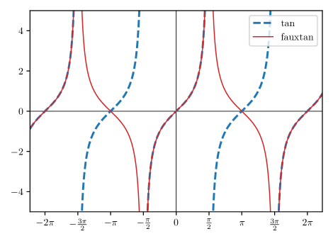
Figure C.1: The modified tangent function $\operatorname{fauxtan}\colon\mathbb{R}\rightarrow\overline{\mathbb{R}}$.

We start with defining the affine function $b_{u}\colon[0,1]\rightarrow\mathbb{R}$ for each $u=(u_{1},u_{2})\in\mathbb{S}$ by the formula

$$b_{u}\colon[0,1]\rightarrow\mathbb{R},\,\begin{cases}0\mapsto\min\,\operatorname{fauxtan}(\{u_{1},u_{2}\})\\ 1\mapsto\max\operatorname{fauxtan}(\{u_{1},u_{2}\}),\end{cases}$$ (C.1)

where ${\operatorname{fauxtan}\colon\mathbb{R}\rightarrow\overline{\mathbb{R}}},$ shown in Fig. C.1, is the unique continous extension of the restricted ordinary tangent function $\tan\colon\left(-\frac{\pi}{2},\frac{\pi}{2}\right)\rightarrow\mathbb{R}$ that is symmetric with respect to translation by $2\pi$ and reflection at $\frac{\pi}{2}$: $\operatorname{fauxtan}(x)=\operatorname{fauxtan}(x+2\pi)=\operatorname{fauxtan}(\pi-x)$ for all $x\in\mathbb{R}$, and $\operatorname{fauxtan}(\pm\frac{\pi}{2})=\pm\infty$. As a side note, for each $u\in R$ we have $\operatorname{Dgm}(b_{u})=\mathbf{1}_{u}$ and hence $b_{u}=f_{u}$.

Next we construct the simplicial complex $X_{u}$ as well as the two simplicial maps $j_{u}\colon[0,1]\rightarrow X_{u}$ and $r_{u}\colon X_{u}\rightarrow[0,1]$ in terms of the corresponding vertex maps for each $u\in\mathbb{I}$. To this end, let $Q:=\uparrow(\frac{\pi}{2},-\frac{\pi}{2})$ be the principal upset of $(\frac{\pi}{2},-\frac{\pi}{2})$. Then $E:=Q\setminus T(Q)$ is a fundamental domain for the $\mathbb{Z}$-action on $\mathbb{M}$, and the map

$$\mathbb{N}_{>0}\times E\rightarrow\mathbb{M}\setminus Q,(n,v)\mapsto T^{-n}(v)$$

is a bijection. Now the intersection

$$E\cap\left(\left(-\frac{\pi}{2},\frac{\pi}{2}\right)^{2}+\pi\mathbb{Z}^{2}\right)$$

has three connected components; namely

$$E_{1} :=E\cap\left(-\frac{3\pi}{2},-\frac{\pi}{2}\right)\times\left(-\frac{\pi}{2},\frac{\pi}{2}\right),$$

$$E_{2} :=E\cap\left(-\frac{\pi}{2},\frac{\pi}{2}\right)\times\left(\frac{\pi}{2},\frac{3\pi}{2}\right),\quad\text{and}$$

$$E_{3} :={\color[rgb]{.828,.828,.828}E}\mathbin{{\color[rgb]{.828,.828,.828}\cap}}\left(-\frac{\pi}{2},\frac{\pi}{2}\right)^{2}$$

as shown in Fig. C.2.

Figure C.2: The three connected components $E_{1}$, $E_{2}$, and $E_{3}$.

Altogether we obtain the bijection

$$\mathbb{N}_{>0}\times(E_{1}\cup E_{2}\cup E_{3})\xrightarrow{~{}\cong~{}}\mathbb{I},~{}(n,v)\mapsto T^{-n}(v).$$

In the following we denote the standard $n$-simplex by $\Delta^{n}$ for $n\in\mathbb{N}_{0}$. Its vertex set is given by the standard basis ${\{e_{0},\dots,e_{n}\}\subset\mathbb{R}^{n+1}}$. Now let ${u\in\mathbb{I}}$ and let ${n\in\mathbb{N}_{>0}}$ such that ${v:=T^{n}(u)\in E}$. We distinguish between three cases depending on which of the three connected components of $E$ contains $v$.

For $v\in E_{1},$

we set

$$X_{u} :=\Lambda^{n+1}_{n+1},$$

$$j_{u} :\,[0,1]\rightarrow X_{u},\,\begin{cases}0\mapsto e_{0}\\ 1\mapsto e_{n+1},\end{cases}$$

$$\text{and}\quad r_{u} :\,X_{u}\rightarrow[0,1],~{}e_{k}\mapsto\begin{cases}0&0\leq k\leq n\\ 1&k=n+1.\end{cases}$$

Here $\Lambda^{n+1}_{n+1}$ is the simplicial complex we obtain from $\partial\Delta^{n+1}$ after removing the facet opposite to the $(n+1)$-st vertex, keeping all other simplices.

For $v\in E_{2},$

we set

$$X_{u} :=\Lambda^{n+1}_{0},$$

$$j_{u} :\,[0,1]\rightarrow X_{u},\,\begin{cases}0\mapsto e_{0}\\ 1\mapsto e_{n+1},\end{cases}$$

$$\text{and}\quad r_{u} :\,X_{u}\rightarrow[0,1],~{}e_{k}\mapsto\begin{cases}0&k=0\\ 1&1\leq k\leq n+1.\end{cases}$$

Here $\Lambda^{n+1}_{0}$ is the simplicial complex we obtain from $\partial\Delta^{n+1}$ after removing the facet opposite to the $0$-th vertex.

For $v\in E_{3}$

the construction is not as direct as in the previous two cases. We start by setting

$$X_{u}:=\left(\partial\Delta^{n+1}\right)\times[0,1]\subset\mathbb{R}^{n+2}\times\mathbb{R}$$

with the following triangulation (which coincides with the triangulation induced by the corresponding simplicial set). The vertex set of $X_{u}$ is $\{e_{0},\dots,e_{n+1}\}\times\{0,1\}$ and a set of pairs in $\{e_{0},\dots,e_{n+1}\}\times\{0,1\}$ spans a simplex in $X_{u}$ iff the index of each basis vector that appears in a pair with $0$ is at most the index of any basis vector that appears in a pair with $1$ and there is one basis vector not appearing in any pair. (The second condition ensures that we are not adding a simplex to $X_{u}$ that is not even contained in the proclaimed underlying space of $X_{u}$.) With this triangulation, we define the simplicial map

$$j_{u} :\,[0,1]\rightarrow X_{u},\,\begin{cases}0\mapsto(e_{0},0)\\ 1\mapsto(e_{n+1},1).\end{cases}$$

To define the retraction $r_{u}\colon X_{u}\rightarrow[0,1]$ we have to distinguish between two cases depending on which of the two coordinates $v_{1}$ and $v_{2}$ of $v=(v_{1},v_{2})$ is larger than or smaller than the other. For $v_{1}\leq v_{2}$ we set

$$r_{u}\colon X_{u}\rightarrow[0,1],~{}(e_{k},l)\mapsto\begin{cases}0&0\leq k\leq n\\ 1&k=n+1\end{cases}$$

and if ${v_{1}>v_{2}}$, then we define $r_{u}$ to be the projection

$$r_{u}:=\operatorname{pr}_{2}\colon\left(\partial\Delta^{n+1}\right)\times[0,1]\rightarrow[0,1],~{}(e_{k},l)\mapsto l$$

onto the second factor. Here the intuition is the following. When $v_{1}=v_{2}$, then $b_{u}\colon[0,1]\rightarrow\mathbb{R}$ is constant, so we can “flip” the retraction $r_{u}\colon X_{u}\rightarrow[0,1]$ without changing the composed map $f_{u}=b_{u}\circ r_{u}$.

Appendix D Sections of Sheaves on Intersections of Open Sets

The sheaf condition essentially says that any compatible family of sections on a cover uniquely glues to a global section. Given a cover by two open subsets, we may conversely ask, which are the sections on the intersection, that can be obtained as the restriction of a section on either of the two open subsets. To this end, let $X$ be a topological space, let $U_{1}\cup U_{2}=X$ be an open cover of $X$, and let $F$ be a sheaf on $X$ with values in the category of abelian groups. We consider the group of sections $F(U_{1}\cap U_{2})$ of $F$ on the intersection of $U_{1}$ and $U_{2}$. Some of these sections can be obtained by restriction from sections of $F$ on $U_{1}$ or $U_{2}$. Thus, there is an induced group homomorphism

$$\nabla_{U_{1},U_{2}}(F)\colon F(U_{1})\oplus F(U_{2})\rightarrow F(U_{1}\cap U_{2}).$$

Now suppose we have open subsets $V_{1},V_{2}\subseteq X$ with $U_{i}\subseteq V_{i}$ for $i=1,2$. Then we have the commutative diagram

(D.1)

as well as the induced map on cokernels $\alpha\colon\mathrm{coker}(\nabla_{V_{1},V_{2}})(F)\rightarrow\operatorname{coker}(\nabla_{U_{1},U_{2}}(F))$.

Lemma D.1.

The map $\alpha\colon\mathrm{coker}(\nabla_{V_{1},V_{2}}(F))\rightarrow\operatorname{coker}(\nabla_{U_{1},U_{2}}(F))$ in the above diagram (D.1) is injective.

Proof.

Identifying $H^{0}(U;F)$ with $F(U)$ for any open subset $U\subseteq X$ and using the Mayer-Vietoris sequence for sheaf cohomology (see for example [KS90, Remark 2.6.10]) we obtain the commutative diagram

with exact columns. By the exactness of these two columns at ${H^{0}(V_{1}\cap V_{2};F)}$ and ${H^{0}(U_{1}\cap U_{2};F)}$ respectively we obtain the commutative diagram

with the two vertical maps monomorphisms of abelian groups as indicated. Thus, the map $\alpha\colon\mathrm{coker}(\nabla_{V_{1},V_{2}}(F))\rightarrow\operatorname{coker}(\nabla_{U_{1},U_{2}}(F))$ is a monomorphism as well. ∎

References

• [BBF21] Ulrich Bauer, Magnus Bakke Botnan, and Benedikt Fluhr. Structure and Interleavings of Relative Interlevel Set Cohomology. arXiv e-prints, 2021.
• [BBF22] Ulrich Bauer, Håvard Bakke Bjerkevik, and Benedikt Fluhr. Quasi-universality of Reeb graph distances. In 38th International Symposium on Computational Geometry (SoCG 2022), volume 224 of LIPIcs. Leibniz Int. Proc. Inform., pages Paper No. 14, 18. Schloss Dagstuhl. Leibniz-Zent. Inform., Wadern, 2022.
• [BdSS15] Peter Bubenik, Vin de Silva, and Jonathan Scott. Metrics for generalized persistence modules. Found. Comput. Math., 15(6):1501–1531, 2015.
• [BdSS17] Peter Bubenik, Vin de Silva, and Jonathan Scott. Interleaving and gromov-hausdorff distance, 2017. Preprint.
• [BEMP13] Paul Bendich, Herbert Edelsbrunner, Dmitriy Morozov, and Amit Patel. Homology and robustness of level and interlevel sets. Homology Homotopy Appl., 15(1):51–72, 2013.
• [BF22] Ulrich Bauer and Benedikt Fluhr. Relative Interlevel Set Cohomology Categorifies Extended Persistence Diagrams. arXiv e-prints, May 2022.
• [BG22] Nicolas Berkouk and Grégory Ginot. A derived isometry theorem for sheaves. Adv. Math., 394:Paper No. 108033, 39, 2022.
• [BGO19] Nicolas Berkouk, Grégory Ginot, and Steve Oudot. Level-sets persistence and sheaf theory. arXiv e-prints, Jul 2019.
• [BLM21] Ulrich Bauer, Claudia Landi, and Facundo Mémoli. The Reeb graph edit distance is universal. Found. Comput. Math., 21(5):1441–1464, 2021.
• [CCF+20] Michael J. Catanzaro, Justin M. Curry, Brittany Terese Fasy, Jānis Lazovskis, Greg Malen, Hans Riess, Bei Wang, and Matthew Zabka. Moduli spaces of Morse functions for persistence. J. Appl. Comput. Topol., 4(3):353–385, 2020.
• [CCLL22] Robert Cardona, Justin Curry, Tung Lam, and Michael Lesnick. The universal $\ell^{p}$-metric on merge trees. In 38th International Symposium on Computational Geometry (SoCG 2022), volume 224 of LIPIcs. Leibniz Int. Proc. Inform., pages Paper No. 24, 20. Schloss Dagstuhl. Leibniz-Zent. Inform., Wadern, 2022.
• [CdM09] Gunnar Carlsson, Vin de Silva, and Dmitriy Morozov. Zigzag persistent homology and real-valued functions. In Proceedings of the Twenty-fifth Annual Symposium on Computational Geometry, SCG ’09, pages 247–256, New York, NY, USA, 2009. ACM.
• [CdSKM19] Gunnar Carlsson, Vin de Silva, Sara Kališnik, and Dmitriy Morozov. Parametrized homology via zigzag persistence. Algebr. Geom. Topol., 19(2):657–700, 2019.
• [CO17] Mathieu Carrière and Steve Oudot. Local equivalence and intrinsic metrics between Reeb graphs. In 33rd International Symposium on Computational Geometry, volume 77 of LIPIcs. Leibniz Int. Proc. Inform., pages Art. No. 25, 15. Schloss Dagstuhl. Leibniz-Zent. Inform., Wadern, 2017.
• [CSEH07] David Cohen-Steiner, Herbert Edelsbrunner, and John Harer. Stability of persistence diagrams. Discrete Comput. Geom., 37(1):103–120, 2007.
• [CSEH09] David Cohen-Steiner, Herbert Edelsbrunner, and John Harer. Extending persistence using Poincaré and Lefschetz duality. Found. Comput. Math., 9(1):79–103, 2009.
• [Cur14] Justin Michael Curry. Sheaves, cosheaves and applications. PhD thesis, University of Pennsylvania, 2014.
• [DeS21] Jordan DeSha. Inverse Problems for Topological Summaries in Topological Data Analysis. PhD thesis, University at Albany, State University of New York, 2021.
• [dSMP16] Vin de Silva, Elizabeth Munch, and Amit Patel. Categorified Reeb graphs. Discrete Comput. Geom., 55(4):854–906, 2016.
• [DW07] Tamal K. Dey and Rephael Wenger. Stability of critical points with interval persistence. Discrete Comput. Geom., 38(3):479–512, 2007.
• [ELZ02] Herbert Edelsbrunner, David Letscher, and Afra Zomorodian. Topological persistence and simplification. Discrete Comput. Geom., 28(4):511–533, 2002.
• [Gab72] Peter Gabriel. Unzerlegbare Darstellungen. I. Manuscripta Math., 6:71–103; correction, ibid. 6 (1972), 309, 1972.
• [Gui16] Stéphane Guillermou. The three cusps conjecture. arXiv e-prints, March 2016.
• [HKLM19] Shaun Harker, Miroslav Kramár, Rachel Levanger, and Konstantin Mischaikow. A comparison framework for interleaved persistence modules. J. Appl. Comput. Topol., 3(1-2):85–118, 2019.
• [KS90] Masaki Kashiwara and Pierre Schapira. Sheaves on manifolds, volume 292 of Grundlehren der mathematischen Wissenschaften [Fundamental Principles of Mathematical Sciences]. Springer-Verlag, Berlin, 1990. With a chapter in French by Christian Houzel.
• [KS18] Masaki Kashiwara and Pierre Schapira. Persistent homology and microlocal sheaf theory. J. Appl. Comput. Topol., 2(1-2):83–113, 2018.
• [Les15] Michael Lesnick. The theory of the interleaving distance on multidimensional persistence modules. Found. Comput. Math., 15(3):613–650, 2015.
• [MP20] Alex McCleary and Amit Patel. Bottleneck stability for generalized persistence diagrams. Proc. Amer. Math. Soc., 148(7):3149–3161, 2020.
• [Sco20] Luis Scoccola. Locally Persistent Categories And Metric Properties Of Interleaving Distances. PhD thesis, Western University, 2020.
• [Spa81] Edwin H. Spanier. Algebraic topology. Springer-Verlag, New York-Berlin, 1981. Corrected reprint.
• [tom08] Tammo tom Dieck. Algebraic topology. EMS Textbooks in Mathematics. European Mathematical Society (EMS), Zürich, 2008.