Near-conformal dynamics in a chirally broken system

Abstract

Composite Higgs models must exhibit very different dynamics from quantum chromodynamics (QCD) regardless whether they describe the Higgs boson as a dilatonlike state or a pseudo-Nambu-Goldstone boson. Large separation of scales and large anomalous dimensions are frequently desired by phenomenological models. Mass-split systems are well-suited for composite Higgs models because they are governed by a conformal fixed point in the ultraviolet but are chirally broken in the infrared. In this work we use lattice field theory calculations with domain wall fermions to investigate a system with four light and six heavy flavors. We demonstrate how a nearby conformal fixed point affects the properties of the four light flavors that exhibit chiral symmetry breaking in the infrared. Specifically we describe hyperscaling of dimensionful physical quantities and determine the corresponding anomalous mass dimension. We obtain $y_{m}=1+\gamma^{*}=1.47(5)$ suggesting that $N_{f}=10$ lies inside the conformal window. Comparing the low energy spectrum to predictions of dilaton chiral perturbation theory, we observe excellent agreement which supports the expectation that the 4+6 mass-split system exhibits near-conformal dynamics with a relatively light $0^{++}$ isosinglet scalar.

I Introduction

Experiments have discovered a $125$ GeV Higgs boson Aad et al. (2012); Chatrchyan et al. (2012); Aad et al. (2015) but so far, up to a few TeV, no direct signs of physics beyond the standard model (BSM) have been seen. The standard model (SM), however, is an effective theory, and new interactions are necessary to UV complete the Higgs sector, explain dark matter, and account for the matter-antimatter asymmetry of the universe. For gauge theories describing the Higgs sector as a composite structure, experimental observations imply that a large separation of scales between the electroweak scale (IR) and new ultraviolet physics (UV) Contino (2011); Luty and Okui (2006); Dietrich and Sannino (2007); Luty (2009); Brower et al. (2016); Csaki et al. (2016); Arkani-Hamed et al. (2016); Witzel (2019) is required. Theories with a large separation of scales part company from QCD, exhibiting a “walking” gauge coupling Yamawaki et al. (1986); Appelquist et al. (1986); Bando et al. (1988), and providing a dynamical mechanism for electroweak (EW) symmetry breaking. They can satisfy stringent constraints from EW precision measurements but avoid unnaturally large tuning of the Higgs mass.

To explore theories with a large scale separation and infrared dynamics different from QCD, we employ the device of mass splitting Brower et al. (2015, 2016); Hasenfratz et al. (2017a, 2018), where the action has two fermion mass parameters: $\widehat{m}_{h}$ and a smaller $\widehat{m}_{\ell}$. The idea is to start with sufficiently many fermions to guarantee that at scales well above the fermion masses the theory exhibits infrared conformality. By assigning the masses $\widehat{m}_{h}$ and $\widehat{m}_{\ell}$ to the fermions, we create a system with $N_{h}$ heavy fermions and $N_{\ell}$ light fermions. The number of light fermions $N_{\ell}$ is chosen such that the light sector alone exhibits spontaneous chiral symmetry breaking. The resulting mass-split theory is governed by the conformal IRFP above the high scale set by $\widehat{m}_{h}$. There the spectrum exhibits conformal hyperscaling, and the mass of the lightest isosinglet scalar $0^{++}$ is expected to be comparable to the corresponding pseudoscalar mass Miransky (1999); Aoki et al. (2013).

In the infrared, the heavy fermions decouple, the gauge coupling runs to larger values, and chiral symmetry for the light flavors breaks spontaneously. The heavy-fermion mass $\widehat{m}_{h}$ controls the separation of scales between the UV and IR Hasenfratz et al. (2018). Even though the low energy theory is chirally broken, its properties are significantly different from a QCD-like theory with $N_{\ell}$ fermions. In particular a light $0^{++}$ state may enter the effective chiral Lagrangian, requiring the extension to dilaton chiral perturbation theory (dChPT) Golterman and Shamir (2016); Appelquist et al. (2018, 2017); Golterman and Shamir (2018); Appelquist et al. (2020); Golterman et al. (2020).

It is favorable to keep the total number of fermions $N_{f}=N_{h}+N_{\ell}$ near the low end of the conformal window to achieve a large anomalous dimension. Specifically we study an $SU(3)$ gauge theory with four light and six heavy fermions in the fundamental representation. Although no consensus has been reached on the precise onset of the conformal window for $SU(3)$ gauge theories with fundamental fermions, there are indications that $N_{f}=10$ is infrared conformal Hayakawa et al. (2011); Appelquist et al. (2012); Chiu (2016, 2017, 2019); Fodor et al. (2018); Hasenfratz et al. (2019, 2020); Baikov et al. (2017); Ryttov and Shrock (2011, 2016a, 2016b, 2017); Antipin et al. (2019); Di Pietro and Serone (2020). By choosing a theory with four fermions in the light, chirally broken sector, our simulations can also directly be related to existing models extending the SM with a new strongly interacting sector Ma and Cacciapaglia (2016); Buarque Franzosi et al. (2020); Marzocca (2018). In these models the Higgs boson is a pseudo-Nambu-Goldstone boson (pNGB) of the new strong sector Vecchi (2017); Ferretti and Karateev (2014); Ferretti (2016); Ma and Cacciapaglia (2016); Buarque Franzosi et al. (2020).

We explore this new, strongly coupled theory by performing large scale numerical lattice-field-theory simulations. The choice $N_{f}=10$ improves over a pilot study using four light and eight heavy flavors Brower et al. (2015, 2016); Hasenfratz et al. (2017a); Brower et al. (2014); Weinberg et al. (2015); Hasenfratz et al. (2017b, 2016, c) by being closer to the bottom of the conformal window. Also, we perform the numerical simulations using chiral domain-wall fermions (DWF) Kaplan (1992); Shamir (1993); Furman and Shamir (1995); Brower et al. (2017) which preserve the flavor structure. While numerically more costly, DWF provide a theoretically clean environment to perform investigations of strongly coupled theories near a conformal IR fixed point.

We briefly introduce the details of the numerical simulations before we demonstrate hyperscaling and determine the mass anomalous dimension. This allows us to explore implications for a possible effective description at low energies. Finally we give an outlook on our future calculations of phenomenologically important quantities. Preliminary results have been reported in Witzel et al. (2018); Witzel and Hasenfratz (2019).

II Numerical simulations

Simulations are performed on hypercubic lattices using $(L/a)^{3}\times T/a$ volumes with $L/a=24$ or 32 and $T/a=64$ where $a$ indicates the lattice spacing. We simulate the $SU(3)$ gauge system with four light and six heavy flavors using the Symanzik gauge action Lüscher and Weisz (1985a, b) with 3-times stout-smeared ($\rho=0.1$) Morningstar and Peardon (2004) Möbius domain wall fermions Brower et al. (2017) ($b_{5}=1.5$, $c_{5}=0.5$). DWF are simulated by adding a fifth dimension of extent $L_{s}$ which separates the physical modes of four dimensional space-time. For practical reasons $L_{s}$ needs to be finite i.e. DWF exhibit a small, residual chiral symmetry breaking, conventionally parametrized as an additive mass term $am_{\text{res}}$. In our simulations we choose $L_{s}=16$ and set the domain wall height $M_{5}=1$. We determine the residual chiral symmetry breaking numerically and find small values of $O({10}^{-3})$. To correctly refer to the dimensionless lattice masses, we introduce the notation

$$\widehat{m}_{x}\equiv a\widetilde{m}_{x}=a(m_{x}+m_{\text{res}})\quad\text{with}\quad x=\ell,\,h.$$ (1)

Based on insight from our accompanying step-scaling investigation Hasenfratz et al. (2019, 2020), we set the bare gauge coupling $\beta=6/g_{0}^{2}=4.03$, close to the IRFP of the underlying conformal theory with ten degenerate flavors. The hybrid Monte Carlo (HMC) update algorithm Duane et al. (1987) with a trajectory length of $\tau=2$ MDTU (molecular dynamics time units) is used to generate ensembles of dynamical gauge field configurations with $1-3$k ($0.3-0.5$k) thermalized trajectories for $am_{\ell}\leq 0.04$ ($am_{\ell}>0.04$). Using input heavy flavor mass $am_{h}=0.200$, 0.175, and 0.150, we explore the 4+6 system choosing five or seven values for the input light flavor mass in the range $0.015\leq am_{\ell}\leq 0.100$. Spectrum measurements are performed every 20 (10) MDTU for $am_{\ell}<0.04$ ($am_{\ell}\geq 0.04$) and we decorrelate subsequent measurements by randomly choosing source positions. Remaining autocorrelations are estimated using the $\Gamma$-method Wolff (2004) and accounted for by correspondingly binning subsequent measurements in our jackknife analysis. For all ensembles we observe frequent changes of the topological charge measured every 10 MDTU (20 MDTU for $m_{\ell}/m_{h}=0.015/0.150$) which typically is a quantity exhibiting the longest autocorrelation times in the system. Examples of the Monte Carlo histories for six high statistics ensembles are shown in Fig. 1.

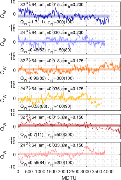
Figure 1: Monte Carlo histories of the topological charge obtained using Wilson gradient flow at flow time $t=L^{2}/32$ for six high statistics ensembles. The integrated autocorrelation time $\tau_{\text{int}}$ of the topological charge $Q_{W}$ is determined using the $\Gamma$-method Wolff (2004) and quoted in units of MDTU.

III Hyperscaling

To understand the properties of mass-split systems, we refer to Wilsonian renormalization group (RG). In the UV both mass parameters are much lighter than the cutoff $\Lambda_{\text{cut}}=1/a$: $\widehat{m}_{l}\ll 1$, $\widehat{m}_{h}\ll 1$. As the energy scale $\mu$ is lowered from the cutoff, the RG flowed lattice action moves in the infinite parameter action space as dictated by the fixed point structure of the $N_{f}$ flavor conformal theory. The masses are increasing according to their scaling dimension $y_{m}$, $\widehat{m}_{\ell,h}\to\widehat{m}_{\ell,h}(a\mu)^{-y_{m}}$, but we assume that they are still small so the system remains close to the conformal critical surface. All other couplings are irrelevant and approach the IRFP as the energy scale is lowered.

If the gauge couplings reach the vicinity of the IRFP, only the two masses change under RG flow. We can use standard hyperscaling arguments DeGrand and Hasenfratz (2009); Del Debbio and Zwicky (2010, 2011) to show that any physical quantity $aM_{H}$ of mass dimension one follows, at leading order, the scaling form Hasenfratz et al. (2017a)

$$aM_{H}=\widehat{m}_{h}^{1/y_{m}}\Phi_{H}(\widehat{m}_{\ell}/\widehat{m}_{h}),$$ (2)

where $y_{m}=1+\gamma_{m}^{\star}$ is the universal scaling dimension of the mass at the IRFP and $\Phi_{H}$ some function of $\widehat{m}_{\ell}/\widehat{m}_{h}$. $\Phi_{H}$ depends on the observable $H$ and could be qualitatively different for different $H$. The scaling relation Eq. (2) is valid as long as the gauge couplings remain at the IRFP and lattice masses are small, i.e. even in the $\widehat{m}_{\ell}=0$ chiral limit. As a consequence, ratios of masses

$$\frac{M_{H1}}{M_{H2}}=\frac{\Phi_{H1}(\widehat{m}_{\ell}/\widehat{m}_{h})}{\Phi_{H2}(\widehat{m}_{\ell}/\widehat{m}_{h})}$$ (3)

depend only on $\widehat{m}_{\ell}/\widehat{m}_{h}$. The heavy flavors decouple when $\widehat{m}_{h}(a\mu)^{-y_{m}}\approx 1$. At that point the light flavors condense and spontaneously break chiral symmetry. This allows us to define the hadronic or chiral symmetry breaking scale

$$\Lambda_{H}=\widehat{m}_{h}^{1/y_{m}}a^{-1}.$$ (4)

As the energy scale $\mu$ is lowered below $\Lambda_{H}$, the gauge coupling starts running again. However, properties of the IRFP are already encoded in hadronic observables.

Figure 2: The inverse Wilson flow scale $a/\sqrt{8t_{0}}$ and interpolating fit according to Eq. (2) as function of $\widehat{m}_{\ell}/\widehat{m}_{h}$. The bottom panel shows “curve collapse” for $\Phi_{\sqrt{8t_{0}}}(\widehat{m}_{\ell}/\widehat{m}_{h})=a/\sqrt{8t_{0}}\cdot\widehat{m}_{h}^{-1/y_{m}}$.

We have established hyperscaling of ratios in the 4+8 flavor system Brower et al. (2016); Hasenfratz et al. (2017a) and preliminary results for the 4+6 system are reported in Witzel et al. (2018); Witzel and Hasenfratz (2019).

In Fig. 2 we illustrate hyperscaling and the determination of $y_{m}$ by considering the inverse Wilson flow scale $a/\sqrt{8t_{0}}$ as the quantity $aM_{H}$ in Eq. (2). The dimensionful quantity $1/\sqrt{8t_{0}}$ is proportional to the energy scale where the renormalized running coupling in the gradient flow scheme equals a reference value ($g^{2}_{GF}\approx 16$) Lüscher (2010). The top panel shows $a/\sqrt{8t_{0}}$ as the function of $\widehat{m}_{\ell}/\widehat{m}_{h}$. While the data corresponding to our three different $am_{h}$ values are different, each set on its own follows a smooth, almost linear curve. This suggests to parametrize the unknown function $\Phi_{\sqrt{8t_{0}}}(\widehat{m}_{\ell}/\widehat{m}_{h})$ using a low-order polynomial and perform a combined fit to all 17 data points in Fig. 2 using the Ansatz given in Eq. (2). A fit with a quadratic polynomial describes our data well. Small deviations of very precise $a/\sqrt{8t_{0}}$ values lead to $\chi^{2}/\text{d.o.f.}\approx 3$ and $y_{m}=1.469(23)$ with likely underestimated statistical uncertainties.

Figure 3: Hyperscaling of the light-light (shaded symbols), heavy-light (open symbols), and heavy-heavy (filled symbols) pseudoscalar decay constant as the function of $\widehat{m}_{\ell}/\widehat{m}_{h}$. A combined fit based on Eq. (2) determines $y_{m}$.

The bottom panel of Fig. 2 shows the data points for $a/\sqrt{8t_{0}}\cdot\widehat{m}_{h}^{-1/y_{m}}$ and the quadratic fit function $\Phi_{\sqrt{8t_{0}}}(\widehat{m}_{\ell}/\widehat{m}_{h})$, exhibiting the expected “curve collapse.” We find similar curve collapse for other observables and show in Fig. 3 the result for a combined, correlated fit to the light-light $(\ell\ell)$, heavy-light $(h\ell)$, and heavy-heavy $(hh)$ pseudoscalar decay constant $aF_{ps}$. Since the determination of $aF_{ps}$ is equally precise for $\ell\ell$, $h\ell$, or $hh$ states, this fit provides a representative determination of $y_{m}$ with a good $p$-value. Subsequently we use

$$y_{m}=1+\gamma_{m}^{\star}=1.470(52),$$ (5)

as our reference value and note it is consistent within uncertainties to determinations from other observables like vector or pseudoscalar masses. Further $y_{m}$ is in agreement to an independent determination based on gradient flow Hasenfratz and Witzel (tion) and comparable to predictions from analytical calculations Ryttov and Shrock (2016c, 2017, 2018). The predicted $\gamma_{m}^{\star}$ is substantially below 1, the value expected for a system close to the sill of the conformal window Yamawaki et al. (1986); Matsuzaki and Yamawaki (2014). Since dChPT analysis of the $N_{f}=8$ data Appelquist et al. (2016, 2019) predicts $\gamma_{m}^{*}$ near 1 Golterman and Shamir (2016); Appelquist et al. (2018, 2017); Golterman and Shamir (2018); Appelquist et al. (2020); Golterman et al. (2020), this indicates the sill of the conformal window lies between $N_{f}=8$ and 10, whereas the 12 flavor system ($\gamma_{m}^{\star}\approx 0.24$ Appelquist et al. (2011); DeGrand (2011); Cheng et al. (2013, 2014); Lombardo et al. (2014); Ryttov and Shrock (2016c, 2017, 2018); Li and Poland (2020)) is even deeper in the conformal regime.

The scaling of $a/\sqrt{8t_{0}}$ is particularly interesting because it shows that the lattice spacing in the $\widehat{m}_{\ell}=0$ chiral limit has a simple dependence on the heavy flavor mass

$$a=(\widehat{m}_{h})^{1/y_{m}}\cdot\Phi_{\sqrt{8t_{0}}}(0)\cdot\sqrt{8t_{0}}|_{m_{\ell}=0},$$ (6)

where $\Phi_{\sqrt{8t_{0}}}(0)$ is a finite number, $\approx 0.48$, in the 4+6 system. This confirms the expectation that the continuum $a=0$ limit is approached as $\widehat{m}_{h}$ decreases. Combined with Eq. (4) it predicts the hadronic scale

$$\Lambda_{H}^{-1}=\Phi_{\sqrt{8t_{0}}}(0)\cdot\sqrt{8t_{0}}|_{m_{\ell}=0}.$$ (7)

IV Low energy effective description

In the low energy infrared limit our system exhibits spontaneous chiral symmetry breaking. It should be described by a chiral effective Lagrangian which smoothly connects to the hyperscaling relation Eq. (2), valid at the hadronic scale $\mu=\Lambda_{H}$. In order to combine data sets with different $\widehat{m}_{h}$, we express the lattice scale $a$ in terms of the hadronic scale $\Lambda_{H}$

$$M_{H}/\Lambda_{H}=(aM_{H})\cdot{\widehat{m}}_{h}^{-1/y_{m}} =\Phi_{H}(\widehat{m}_{\ell}/\widehat{m}_{h}).$$ (8)

Below the hadronic scale $\Lambda_{H}$, the 4+6 system reduces to a chirally broken $N_{f}=4$ system. The low energy effective theory (EFT) expresses the dependence of physical quantities on the running fermion mass $m_{f}$ of the light flavors. At the hadronic energy scale the light flavor mass in lattice units is $\widehat{m}_{\ell}(a\Lambda_{H})^{-y_{m}}$, predicting

$$m_{f}\propto\widehat{m}_{\ell}(a\Lambda_{H})^{-y_{m}}\cdot\Lambda_{H}=(\widehat{m}_{\ell}/\widehat{m}_{h})\cdot\Lambda_{H}.$$ (9)

The continuum limit is taken by tuning $\widehat{m}_{h}\to 0$ while keeping $\widehat{m}_{\ell}/\widehat{m}_{h}$ fixed.

For $\widehat{m}_{\ell}/\widehat{m}_{h}\lesssim 1$, we expect the $0^{++}$ ground state to be dominated by the light fermions. It is confined at scales of order $\Lambda_{H}$ as are the other states, but its mass could well be small, comparable to the $\ell\ell$ pseudoscalar mass. An EFT describing the small mass regime then needs to incorporate the light scalar state together with the pseudoscalars. In the $m_{f}=0$ limit, only the pseudoscalar states are massless. The $0^{++}$ decouples at very low energies and $N_{f}=4$ ChPT should describe the data.

The dChPT Lagrangian incorporates the effect of a light dilaton state Golterman and Shamir (2016); Appelquist et al. (2018, 2017); Golterman and Shamir (2018); Appelquist et al. (2020); Golterman et al. (2020). While derived for a chirally broken system with degenerate fermions just below the conformal window, we explore its application to our near-conformal mass-split system.

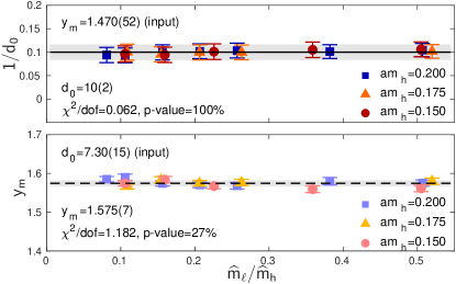
Figure 4: Scaling test of dChPT exploiting Eq. (11). The top panel uses $y_{m}$ (Eq. (5)) as input to fit $1/d_{0}$, the bottom panel shows a fit for $y_{m}$ from a scan over $d_{0}$ values used as input.

dChPT predicts the scaling relation

$$d_{0}\cdot F_{ps}^{2-y_{m}}=M_{ps}^{2}/m_{f},$$ (10)

which is a general result first discussed in Refs. Golterman and Shamir (2016); Appelquist et al. (2017) and independent of the specific form of the dilaton effective potential. The quantity $d_{0}$ is a combination of low energy constants. Using Eq. (8) we express this relation in terms of lattice quantities of the light sector (dropping the superscripts $\ell\ell$)

$$d_{0}\cdot(aF_{ps})^{2-y_{m}}=(aM_{ps})^{2}/\widehat{m}_{\ell}.$$ (11)

From Eq. (2) we can deduce that $d_{0}=(aM_{ps})^{2}\cdot(aF_{ps})^{-2+y_{m}}/\widehat{m}_{\ell}$ may only depend on $\widehat{m}_{\ell}/\widehat{m}_{h}$, whereas Eq. (10) states $d_{0}$ is a constant.

Since our main goal is to study Eq. (10), we simply fix $y_{m}$ from Eq. (5) and determine $d_{0}$ using Eq. (11). As shown in the top panel of Fig. 4, our data form a flat line without dependence on $\widehat{m}_{\ell}/\widehat{m}_{h}$. A direct fit of our data to Eq. (11) to determine $y_{m}$ and $d_{0}$ simultaneously is troublesome because $aF_{ps}$ and $aM_{ps}$ have similar size uncertainties, are highly correlated, and the relation is nonlinear. Instead we perform a second test scanning a range of input values for $d_{0}$ and fit for $y_{m}$. At a minimum $\chi^{2}/\text{d.o.f.}$ we obtain a $y_{m}=1.575(7)$ within $2\sigma$ of our reference value and shown in the lower panel of Fig. 4. In summary, our data are consistent with Eq. (11) and we obtain a rough estimate of $y_{m}$ and $d_{0}$.

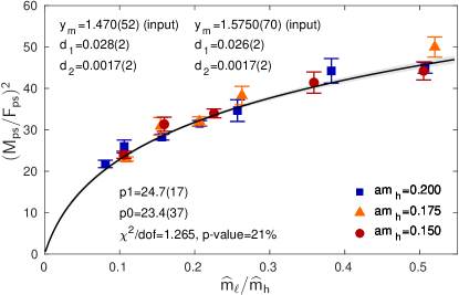
Figure 5: Test of dChPT using Eq. (12). The black line with gray band is fitting our ratios $(M_{ps}/F_{ps})^{2}$ to the function $y=p_{0}W_{0}(p_{1}\cdot\widehat{m}_{\ell}/\widehat{m}_{h})$.

Assuming a specific form of the dilaton potential leads to another dChPT relation Golterman et al. (2020)

$$\frac{M_{ps}^{2}}{F_{ps}^{2}}=\frac{1}{y_{m}d_{1}}W_{0}\left(\frac{y_{m}d_{1}}{d_{2}}m_{f}\right)$$ (12)

where $W_{0}$ is the Lambert W-function and $d_{1}$, $d_{2}$ are mass independent constants. Figure 5 shows a fit of our data to Eq. (12). The fit has an excellent $p$-value and allows us to determine the constants $d_{1}$ and $d_{2}$. Relations of $N_{f}=4$ ChPT at leading and next-to-leading order exhibit a mass dependence different from Eqs. (10) and (12) and do not describe our data.

Finally we comment on the mass dependence of $\sqrt{8t_{0}}/a$. In ChPT this quantity has a linear mass dependence and corrections enter only at NNLO Bär and Golterman (2014). So far dChPT does not provide a useful description for $\sqrt{8t_{0}}/a$ Golterman et al. (2020). Our results in Fig. 2 show however that $a/\sqrt{8t_{0}}$ obeys the usual hyperscaling relation in mass-split systems and $a\sqrt{8t_{0}}\cdot{\widehat{m}_{h}}^{-1/y_{m}}$ is well described by a linear mass dependence.

V Conclusion

In this work we highlight the unique features of the 4+6 mass-split system built on a conformal IRFP. We show that physical masses exhibit hyperscaling and determine the universal mass scaling dimension of the corresponding $N_{f}=10$ system $y_{m}=1+\gamma_{m}^{\star}=1.47(5)$. This value is smaller than expected for a theory near the edge of the conformal window suggesting that $N_{f}=9$ or 8 flavor models could be closer to the sill of the conformal window.

We compare our numerical results to predictions based on dChPT relations and find good agreement. Leading and next-to-leading order standard $N_{f}=4$ ChPT is, however, not consistent with our data. This strongly suggests that the $0^{++}$ isosinglet scalar of the 4+6 mass-split system is a light state for the investigated parameter range.

There are many important questions to be studied in the future. Numerically determining the $0^{++}$ scalar mass has the highest priority. Investigation of the baryonic anomalous dimension, relevant for partial compositeness, is already in progress Hasenfratz and Witzel (tion). Calculations of the $S$ parameter and the Higgs potential are planned as well. Finite temperature studies could identify phase transitions with potentially significant implications for the early universe.

References

- Aad et al. (2012) G. Aad et al. (ATLAS), Phys.Lett. B716, 1 (2012), arXiv:1207.7214 [hep-ex] .
- Chatrchyan et al. (2012) S. Chatrchyan et al. (CMS), Phys.Lett. B716, 30 (2012), arXiv:1207.7235 [hep-ex] .
- Aad et al. (2015) G. Aad et al. (ATLAS, CMS), Phys. Rev. Lett. 114, 191803 (2015), arXiv:1503.07589 [hep-ex] .
- Contino (2011) R. Contino, Proceedings TASI 09, 235 (2011), arXiv:1005.4269 [hep-ph] .
- Luty and Okui (2006) M. A. Luty and T. Okui, JHEP 09, 070 (2006), arXiv:hep-ph/0409274 [hep-ph] .
- Dietrich and Sannino (2007) D. D. Dietrich and F. Sannino, Phys. Rev. D75, 085018 (2007), arXiv:hep-ph/0611341 [hep-ph] .
- Luty (2009) M. A. Luty, JHEP 04, 050 (2009), arXiv:0806.1235 [hep-ph] .
- Brower et al. (2016) R. C. Brower, A. Hasenfratz, C. Rebbi, E. Weinberg, and O. Witzel, Phys. Rev. D93, 075028 (2016), arXiv:1512.02576 [hep-ph] .
- Csaki et al. (2016) C. Csaki, C. Grojean, and J. Terning, Rev. Mod. Phys. 88, 045001 (2016), arXiv:1512.00468 [hep-ph] .
- Arkani-Hamed et al. (2016) N. Arkani-Hamed, R. T. D’Agnolo, M. Low, and D. Pinner, JHEP 11, 082 (2016), arXiv:1608.01675 [hep-ph] .
- Witzel (2019) O. Witzel, PoS LATTICE2018, 006 (2019), arXiv:1901.08216 [hep-lat] .
- Yamawaki et al. (1986) K. Yamawaki, M. Bando, and K.-i. Matumoto, Phys. Rev. Lett. 56, 1335 (1986).
- Appelquist et al. (1986) T. W. Appelquist, D. Karabali, and L. Wijewardhana, Phys. Rev. Lett. 57, 957 (1986).
- Bando et al. (1988) M. Bando, T. Kugo, and K. Yamawaki, Phys. Rept. 164, 217 (1988).
- Brower et al. (2015) R. C. Brower, A. Hasenfratz, C. Rebbi, E. Weinberg, and O. Witzel, J. Exp. Theor. Phys. 120, 423 (2015), arXiv:1410.4091 [hep-lat] .
- Hasenfratz et al. (2017a) A. Hasenfratz, C. Rebbi, and O. Witzel, Phys. Lett. B773, 86 (2017a), arXiv:1609.01401 [hep-ph] .
- Hasenfratz et al. (2018) A. Hasenfratz, C. Rebbi, and O. Witzel, EPJ Web Conf. 175, 08007 (2018), arXiv:1710.08970 [hep-lat] .
- Miransky (1999) V. A. Miransky, Phys. Rev. D59, 105003 (1999), arXiv:hep-ph/9812350 [hep-ph] .
- Aoki et al. (2013) Y. Aoki, T. Aoyama, M. Kurachi, T. Maskawa, K.-i. Nagai, H. Ohki, E. Rinaldi, A. Shibata, K. Yamawaki, and T. Yamazaki (LatKMI), Phys. Rev. Lett. 111, 162001 (2013), arXiv:1305.6006 [hep-lat] .
- Golterman and Shamir (2016) M. Golterman and Y. Shamir, Phys. Rev. D94, 054502 (2016), arXiv:1603.04575 [hep-ph] .
- Appelquist et al. (2018) T. Appelquist, J. Ingoldby, and M. Piai, JHEP 03, 039 (2018), arXiv:1711.00067 [hep-ph] .
- Appelquist et al. (2017) T. Appelquist, J. Ingoldby, and M. Piai, JHEP 07, 035 (2017), arXiv:1702.04410 [hep-ph] .
- Golterman and Shamir (2018) M. Golterman and Y. Shamir, Phys. Rev. D98, 056025 (2018), arXiv:1805.00198 [hep-ph] .
- Appelquist et al. (2020) T. Appelquist, J. Ingoldby, and M. Piai, Phys. Rev. D 101, 075025 (2020), arXiv:1908.00895 [hep-ph] .
- Golterman et al. (2020) M. Golterman, E. T. Neil, and Y. Shamir, Phys. Rev. D 102, 034515 (2020), arXiv:2003.00114 [hep-ph] .
- Hayakawa et al. (2011) M. Hayakawa, K.-I. Ishikawa, Y. Osaki, S. Takeda, S. Uno, and N. Yamada, Phys. Rev. D 83, 074509 (2011), arXiv:1011.2577 [hep-lat] .
- Appelquist et al. (2012) T. Appelquist et al., (2012), arXiv:1204.6000 [hep-ph] .
- Chiu (2016) T.-W. Chiu, (2016), arXiv:1603.08854 [hep-lat] .
- Chiu (2017) T.-W. Chiu, PoS LATTICE2016, 228 (2017).
- Chiu (2019) T.-W. Chiu, Phys. Rev. D99, 014507 (2019), arXiv:1811.01729 [hep-lat] .
- Fodor et al. (2018) Z. Fodor, K. Holland, J. Kuti, D. Nogradi, and C. H. Wong, Phys. Lett. B779, 230 (2018), arXiv:1710.09262 [hep-lat] .
- Hasenfratz et al. (2019) A. Hasenfratz, C. Rebbi, and O. Witzel, Phys. Lett. B798, 134937 (2019), arXiv:1710.11578 [hep-lat] .
- Hasenfratz et al. (2020) A. Hasenfratz, C. Rebbi, and O. Witzel, Phys. Rev. D 101, 114508 (2020), arXiv:2004.00754 [hep-lat] .
- Baikov et al. (2017) P. A. Baikov, K. G. Chetyrkin, and J. H. Kühn, Phys. Rev. Lett. 118, 082002 (2017), arXiv:1606.08659 [hep-ph] .
- Ryttov and Shrock (2011) T. A. Ryttov and R. Shrock, Phys. Rev. D83, 056011 (2011), arXiv:1011.4542 .
- Ryttov and Shrock (2016a) T. A. Ryttov and R. Shrock, Phys. Rev. D94, 105015 (2016a), arXiv:1607.06866 [hep-th] .
- Ryttov and Shrock (2016b) T. A. Ryttov and R. Shrock, Phys. Rev. D94, 125005 (2016b), arXiv:1610.00387 [hep-th] .
- Ryttov and Shrock (2017) T. A. Ryttov and R. Shrock, Phys. Rev. D95, 105004 (2017), arXiv:1703.08558 [hep-th] .
- Antipin et al. (2019) O. Antipin, A. Maiezza, and J. C. Vasquez, Nucl. Phys. B 941, 72 (2019), arXiv:1807.05060 [hep-th] .
- Di Pietro and Serone (2020) L. Di Pietro and M. Serone, JHEP 07, 049 (2020), arXiv:2003.01742 [hep-th] .
- Ma and Cacciapaglia (2016) T. Ma and G. Cacciapaglia, JHEP 03, 211 (2016), arXiv:1508.07014 [hep-ph] .
- Buarque Franzosi et al. (2020) D. Buarque Franzosi, G. Cacciapaglia, and A. Deandrea, Eur. Phys. J. C 80, 28 (2020), arXiv:1809.09146 [hep-ph] .
- Marzocca (2018) D. Marzocca, JHEP 07, 121 (2018), arXiv:1803.10972 [hep-ph] .
- Vecchi (2017) L. Vecchi, JHEP 02, 094 (2017), arXiv:1506.00623 [hep-ph] .
- Ferretti and Karateev (2014) G. Ferretti and D. Karateev, JHEP 03, 077 (2014), arXiv:1312.5330 [hep-ph] .
- Ferretti (2016) G. Ferretti, JHEP 06, 107 (2016), arXiv:1604.06467 [hep-ph] .
- Brower et al. (2014) R. C. Brower, A. Hasenfratz, C. Rebbi, E. Weinberg, and O. Witzel, PoS LATTICE2014, 254 (2014), arXiv:1411.3243 [hep-lat] .
- Weinberg et al. (2015) E. Weinberg, R. C. Brower, A. Hasenfratz, C. Rebbi, and O. Witzel, J. Phys. Conf. Ser. 640, 012055 (2015), arXiv:1412.2148 [hep-lat] .
- Hasenfratz et al. (2017b) A. Hasenfratz, R. Brower, C. Rebbi, E. Weinberg, and O. Witzel, Int. J. Mod. Phys. A 32, 1747003 (2017b), arXiv:1510.04635 [hep-lat] .
- Hasenfratz et al. (2016) A. Hasenfratz, C. Rebbi, and O. Witzel, PoS LATTICE2016, 226 (2016), arXiv:1611.07427 [hep-lat] .
- Hasenfratz et al. (2017c) A. Hasenfratz, C. Rebbi, and O. Witzel, PoS EPS-HEP2017, 356 (2017c), arXiv:1710.02131 [hep-ph] .
- Kaplan (1992) D. B. Kaplan, Phys. Lett. B288, 342 (1992), arXiv:hep-lat/9206013 .
- Shamir (1993) Y. Shamir, Nucl. Phys. B406, 90 (1993), arXiv:hep-lat/9303005 .
- Furman and Shamir (1995) V. Furman and Y. Shamir, Nucl. Phys. B439, 54 (1995), arXiv:hep-lat/9405004 .
- Brower et al. (2017) R. C. Brower, H. Neff, and K. Orginos, Comput. Phys. Commun. 220, 1 (2017), arXiv:1206.5214 [hep-lat] .
- Witzel et al. (2018) O. Witzel, A. Hasenfratz, and C. Rebbi, (2018), arXiv:1810.01850 [hep-ph] .
- Witzel and Hasenfratz (2019) O. Witzel and A. Hasenfratz (Lattice Strong Dynamics), PoS LATTICE2019, 115 (2019), arXiv:1912.12255 [hep-lat] .
- Lüscher and Weisz (1985a) M. Lüscher and P. Weisz, Commun. Math. Phys. 97, 59 (1985a), [Erratum: Commun. Math. Phys.98,433(1985)].
- Lüscher and Weisz (1985b) M. Lüscher and P. Weisz, Phys. Lett. 158B, 250 (1985b).
- Morningstar and Peardon (2004) C. Morningstar and M. J. Peardon, Phys. Rev. D69, 054501 (2004), arXiv:hep-lat/0311018 [hep-lat] .
- Duane et al. (1987) S. Duane, A. Kennedy, B. Pendleton, and D. Roweth, Phys.Lett. B195, 216 (1987).
- Wolff (2004) U. Wolff (ALPHA), Comput.Phys.Commun. 156, 143 (2004), arXiv:hep-lat/0306017 [hep-lat] .
- DeGrand and Hasenfratz (2009) T. DeGrand and A. Hasenfratz, Phys. Rev. D80, 034506 (2009), arXiv:0906.1976 [hep-lat] .
- Del Debbio and Zwicky (2010) L. Del Debbio and R. Zwicky, Phys. Rev. D82, 014502 (2010), arXiv:1005.2371 [hep-ph] .
- Del Debbio and Zwicky (2011) L. Del Debbio and R. Zwicky, Phys. Lett. B 700, 217 (2011), arXiv:1009.2894 [hep-ph] .
- Lüscher (2010) M. Lüscher, JHEP 1008, 071 (2010), arXiv:1006.4518 [hep-lat] .
- Hasenfratz and Witzel (tion) A. Hasenfratz and O. Witzel, “The running anomalous dimension of fermion bi- and trilinear operators in the 10-flavor SU(3) system,” (2020, in preparation), in preparation.
- Ryttov and Shrock (2016c) T. A. Ryttov and R. Shrock, Phys. Rev. D 94, 105014 (2016c), arXiv:1608.00068 [hep-th] .
- Ryttov and Shrock (2018) T. A. Ryttov and R. Shrock, Phys. Rev. D 97, 025004 (2018), arXiv:1710.06944 [hep-th] .
- Matsuzaki and Yamawaki (2014) S. Matsuzaki and K. Yamawaki, Phys. Rev. Lett. 113, 082002 (2014), arXiv:1311.3784 [hep-lat] .
- Appelquist et al. (2016) T. Appelquist, R. Brower, G. Fleming, A. Hasenfratz, X.-Y. Jin, J. Kiskis, E. Neil, J. Osborn, C. Rebbi, E. Rinaldi, D. Schaich, P. Vranas, E. Weinberg, and O. Witzel (Lattice Strong Dynamics), Phys. Rev. D93, 114514 (2016), arXiv:1601.04027 [hep-lat] .
- Appelquist et al. (2019) T. Appelquist, R. Brower, G. Fleming, A. Gasbarro, A. Hasenfratz, X.-Y. Jin, E. Neil, J. Osborn, C. Rebbi, E. Rinaldi, D. Schaich, P. Vranas, E. Weinberg, and O. Witzel (Lattice Strong Dynamics), Phys. Rev. D99, 014509 (2019), arXiv:1807.08411 [hep-lat] .
- Appelquist et al. (2011) T. Appelquist, G. Fleming, M. Lin, E. Neil, and D. Schaich, Phys.Rev. D84, 054501 (2011), arXiv:1106.2148 [hep-lat] .
- DeGrand (2011) T. DeGrand, Phys.Rev. D84, 116901 (2011), arXiv:1109.1237 [hep-lat] .
- Cheng et al. (2013) A. Cheng, A. Hasenfratz, G. Petropoulos, and D. Schaich, JHEP 1307, 061 (2013), arXiv:1301.1355 [hep-lat] .
- Cheng et al. (2014) A. Cheng, A. Hasenfratz, Y. Liu, G. Petropoulos, and D. Schaich, Phys.Rev. D90, 014509 (2014), arXiv:1401.0195 [hep-lat] .
- Lombardo et al. (2014) M. P. Lombardo, K. Miura, T. J. N. da Silva, and E. Pallante, JHEP 12, 183 (2014), arXiv:1410.0298 [hep-lat] .
- Li and Poland (2020) Z. Li and D. Poland, (2020), arXiv:2005.01721 [hep-th] .
- Bär and Golterman (2014) O. Bär and M. Golterman, Phys. Rev. D 89, 034505 (2014), [Erratum: Phys.Rev.D 89, 099905 (2014)], arXiv:1312.4999 [hep-lat] .