Entanglement Hamiltonians for non-critical quantum chains

Abstract

We study the entanglement Hamiltonian for finite intervals in infinite quantum chains for two different free-particle systems: coupled harmonic oscillators and fermionic hopping models with dimerization. Working in the ground state, the entanglement Hamiltonian describes again free bosons or fermions and is obtained from the correlation functions via high-precision numerics for up to several hundred sites. Far away from criticality, the dominant on-site and nearest-neighbour terms have triangular profiles that can be understood from the analytical results for a half-infinite interval. Near criticality, the longer-range couplings, although small, lead to a more complex picture. A comparison between the exact spectra and entanglement entropies and those resulting from the dominant terms in the Hamiltonian is also reported.

1 Introduction

To study the entanglement properties of quantum systems, one divides the full system into two parts and determines how they are coupled in the chosen state [1, 2, 3, 4]. This information is encoded in the reduced density matrix $\rho$ of one of the pieces, and this quantity can always be written in the form $\rho=\exp(-\mathcal{H})/Z$. One therefore is dealing with a kind of statistical mechanics problem, but the operator $\mathcal{H}$, called the entanglement Hamiltonian, depends on the quantum state in question as well as on the type of partition and differs in general from the physical Hamiltonian of the subsystem.

For chains in their ground state, the simplest case is an infinite system divided into two half-infinite ones. Then $\mathcal{H}$ is an operator in which the terms increase linearly as one moves away from the interface. For continuous critical systems, this result is attributed to Bisognano and Wichmann [5, 6] and described by the formula

$$\mathcal{H}=2\pi\int_{0}^{\infty}dx\,x\,\mathcal{T}_{00}(x)$$ (1)

where $\mathcal{T}_{00}(x)$ is the energy density in the physical Hamiltonian. This formula already contains the essence of the situation: the operator $\mathcal{H}$ describes an inhomogeneous system with small terms near the boundary and large ones in the interior of the subsystem. This also holds for the non-critical case, both in the continuum and on a lattice. In the latter case it follows, for integrable chains, from the relation of $\rho$ to corner transfer matrices (CTMs) [7, 8, 2] and the particular structure of these matrices first noted by Baxter [9, 10, 11]. Roughly speaking, the linear increase reflects the geometrical widening of the annular sections in the associated two-dimensional partition functions as the distance from the corner increases.

For other partitions and geometries of continuous critical systems, the form of $\mathcal{H}$ can be obtained from conformal invariance [12, 13, 14, 15]. For example, a subsystem in the form of an interval of length $\ell$ in an infinite chain leads to

$$\mathcal{H}=2\pi\ell\int_{0}^{\ell}dx\,\beta(x)\,\mathcal{T}_{00}(x)$$ (2)

where the parabola $\beta(x)=x/\ell(1-x/\ell)$ increases linearly at both ends of the interval. This has been checked in various numerical calculations. For free fermions on a lattice, one finds that $\mathcal{H}$ contains nearest-neighbour hopping which does not quite vary parabolically and, in addition, hopping to more distant neighbours with smaller amplitudes [2, 16]. However, it has been shown numerically [17] and also analytically [18] that by properly including the longer-range terms in the continuum limit one recovers the conformal result for $\beta(x)$. The same was found for free bosons in the form of coupled harmonic oscillators [19]. Some results also exist for small intervals in interacting fermion systems [20, 21].

The goal of the present work is to characterize $\mathcal{H}$ for an interval in chains away from criticality, and we do this by studying two free-particle models which are generalizations of those just mentioned. For the bosons, the frequency $\omega$ of each single oscillator is kept finite, while for the fermions a dimerization is introduced via alternating hopping matrix elements $t(1\pm\delta)$. This corresponds to the Su-Schrieffer-Heeger model for polyacetylene in the absence of interactions [22, 23]. In both cases, the ground states have Gaussian nature and $\mathcal{H}$ is a free-particle Hamiltonian which can be determined from the correlation functions of the chains [24, 2]. This is done with high-precision numerics which allows to treat large intervals. Both chains can also be related to integrable two-dimensional models which leads to explicit formulae for $\mathcal{H}$ if the interval is half-infinite.

We find that the basic pattern is always similar to the critical case: there are some dominant terms in $\mathcal{H}$ whereas all others are much smaller. In the bosonic case, these are the diagonal matrix elements in the kinetic and in the potential energy and the nearest-neighbour coupling in the latter, while in the fermionic model at half filling, it is the nearest-neighbour hopping. These quantities vanish linearly at the ends of the interval, and the linear behaviour extends more and more into the interior, as one moves away from criticality. In the end, the curves approach a triangular form instead of a parabola. This corresponds to a combination of the effects from the two boundaries, and the slopes are given correctly by the CTM results for the half-infinite subsystem. Defining an approximate entanglement Hamiltonian with these dominant terms, one finds that, except at the upper end, its spectrum is identical to that of the true one. Therefore, it also gives the same entanglement entropy except very close to criticality. These features are completely analogous to those found for critical chains with a parabolic variation of the couplings in $\mathcal{H}$ [25, 26, 27].

In the fermionic case, there is an additional feature due to the dimerization: the dimerization pattern of the physical Hamiltonian is found again in the entanglement Hamiltonian, as already noted in [28]. The even and odd bonds differ, and this is particularly marked in the centre, but both show a trend towards a triangular variation as the dimerization increases. In contrast to the critical case, however, an operator constructed from them commutes only approximately with the entanglement Hamiltonian.

The behaviour of the small matrix elements, which describe longer-range couplings, is more complex. They show spatial oscillations which are absent at criticality and can vanish outside a region around the middle of the interval. A particular subset corresponds to couplings across the centre. The region where they have relatively large values has its maximal extent when the correlation length is comparable to the size of the interval. Because of these features we were not able to obtain a consistent continuum picture near the critical point.

The layout of the paper is as follows. In section 2, we describe the setting and give the basic formulae, in particular for the elements of the correlation functions. Section 3 presents explicit expressions for the entanglement Hamiltonians of half-infinite subsystems, which serve as points of reference for the case of an interval. In section 4, the numerical results for the elements in $\mathcal{H}$ are presented for intervals in strongly non-critical oscillator chains and a simplified version of $\mathcal{H}$ is discussed. In section 5, the same is done for the dimerized hopping chain. Section 6 is devoted to the general features of $\mathcal{H}$ in the non-critical region, including long-range couplings across the middle of the interval, while section 7 sums up our findings and also addresses the question of a continuum limit. Finally, in appendices A and B, the entanglement entropy and the continuum form of $\mathcal{H}$ are derived for a half-infinite subsystem of the oscillator chain, while appendix C discusses a fermionic operator which almost commutes with $\mathcal{H}$.

2 Setting

In this section, we describe the two chains we shall study and give the formulae from which the entanglement Hamiltonian $\mathcal{H}$ follows. For a subsystem of $N$ sites, its diagonal form reads

$$\mathcal{H}=\sum_{l=1}^{N}\varepsilon_{l}\,f_{l}^{{\dagger}}f^{\phantom{{\dagger}}}_{l}$$ (3)

where $f_{l}^{{\dagger}}$ and $f_{l}$ are either bosonic or fermionic creation and annihilation operators and $\varepsilon_{l}$ denote the single-particle eigenvalues. They are determined via elementary correlation matrices restricted to the given segment in the quantum chain at hand, with the relation depending on the particle statistics. In order to obtain the entanglement Hamiltonian in real space, the operators $f_{l}^{{\dagger}}$ and $f_{l}$ have to be transformed back into the original variables, which is again model dependent. In the following we present the two cases separately.

2.1 Harmonic chain

The harmonic chain is a set of coupled oscillators defined by the Hamiltonian

$$\hat{H}=\sum_{n=-\infty}^{+\infty}\left(\frac{1}{2m}\,p_{n}^{2}+\frac{m\omega^{2}}{2}\,q_{n}^{2}+\frac{K}{2}(q_{n+1}-q_{n})^{2}\right)$$ (4)

where $m$ is the mass of the oscillators, $K$ is the nearest-neighbour coupling, while the frequency $\omega$ characterizes the confining potential at each site. The position and momentum operators satisfy the commutation relations $\left[q_{n},p_{m}\right]=i\delta_{n,m}$. The Hamiltonian can be simplified by the canonical transformation $p_{n}\to(mK)^{1/4}\,\hat{p}_{n}$ and $q_{n}\to(mK)^{-1/4}\,\hat{q}_{n}$, which brings (4) into

$$\hat{H}=\sqrt{K/m}\,\sum_{n=-\infty}^{+\infty}\frac{1}{2}\left(\hat{p}_{n}^{2}+\frac{\omega^{2}}{K/m}\,\hat{q}_{n}^{2}+(\hat{q}_{n+1}-\hat{q}_{n})^{2}\right).$$ (5)

Note that, working in units of $\hbar=1$, the overall prefactor $\sqrt{K/m}$ has the dimension of energy, thus the transformation corresponds to working with dimensionless positions, momenta and frequency measured in units of $\sqrt{K/m}$. For simplicity, in our numerical calculations we shall set $K=m=1$, which fixes the energy scale and leaves us with a single parameter $\omega$ to be varied.

The ground state of the harmonic chain can be fully characterized by the correlation functions of positions and momenta. They can be obtained by standard procedure, via introducing bosonic creation/annihilation operators and their Fourier modes, which bring the Hamiltonian into a diagonal form. The calculation of the correlations is then straightforward and yields

$$\langle\hat{q}_{n}\hat{q}_{m}\rangle = \int_{-\pi}^{\pi}\frac{dq}{4\pi}\frac{\cos[q(n-m)]}{\sqrt{\omega^{2}+4\big{[}\sin(q/2)\big{]}^{2}}}$$ (6)

$$\rule{0.0pt}{25.6073pt}\langle\hat{p}_{n}\hat{p}_{m}\rangle = \int_{-\pi}^{\pi}\frac{dq}{4\pi}\sqrt{\omega^{2}+4\big{[}\sin(q/2)\big{]}^{2}}\;\cos[q(n-m)]\,.$$ (7)

The correlation matrices are symmetric and translational invariant, thus their elements depend only on the distance $r=|m-n|$ between the sites. Since in our numerical calculations the matrix elements will be needed to a very high precision, it is useful to have a closed form analytical expression which was reported in [29]

$$\langle\hat{q}_{n}\hat{q}_{n+r}\rangle\,=\,\frac{\kappa^{r+1/2}}{2}\,\frac{\Gamma(r+1/2)}{\Gamma(1/2)\,\Gamma(r+1)}\,_{2}F_{1}\big{(}1/2\,,r+1/2\,,r+1\,,\kappa^{2}\,\big{)}$$ (8)

$$\langle\hat{p}_{n}\hat{p}_{n+r}\rangle\,=\,\frac{\kappa^{r-1/2}}{2}\,\frac{\Gamma(r-1/2)}{\Gamma(-1/2)\,\Gamma(r+1)}\,_{2}F_{1}\big{(}-1/2\,,r-1/2\,,r+1\,,\kappa^{2}\,\big{)}\,.$$ (9)

Here ${}_{2}F_{1}$ is the ordinary hypergeometric function and the parameter $\kappa$ is defined as

$$\kappa\equiv\frac{1}{4}\big{(}\sqrt{\omega^{2}+4}-\omega\,\big{)}^{2}.$$ (10)

Note that $0<\kappa<1$, and thus the correlations in (8) and (9) decay exponentially, with the inverse correlation length given by $\xi^{-1}=-\ln\kappa$. In particular, $\kappa\to 1$ yields the critical point corresponding to the choice $\omega\to 0$, where the matrix elements in (8) become divergent due to the zero mode.

In order to construct the entanglement Hamiltonian, one first introduces the reduced correlation matrices $Q$ and $P$ by restricting the indices in (6) and (7) to the segment $[1,N]$, where the notation $i,j$ will be used. The single-particle spectrum in (3) is then obtained via the Williamson decomposition of the block-diagonal matrix $Q\oplus P$, which tells us that

$$(2Q)\,\phi_{l}=\coth\left(\frac{\varepsilon_{l}}{2}\right)\psi_{l}\;,\;\;\qquad\;\;(2P)\,\psi_{l}=\coth\left(\frac{\varepsilon_{l}}{2}\right)\phi_{l}$$ (11)

where the vectors $\phi_{l}$ and $\psi_{l}$ must satisfy the orthonormality conditions

$$\sum_{i=1}^{N}\phi_{l}(i)\,\psi_{k}(i)=\delta_{l,k}\,,\qquad\sum_{l=1}^{N}\phi_{l}(i)\,\psi_{l}(j)=\delta_{i,j}\,.$$ (12)

The equations (11) imply the following pair of eigenvalue equations

$$(4PQ)\,\phi_{l}=\coth^{2}\left(\frac{\varepsilon_{l}}{2}\right)\phi_{l}\;,\;\;\qquad\;\;(4QP)\,\psi_{l}=\coth^{2}\left(\frac{\varepsilon_{l}}{2}\right)\psi_{l}$$ (13)

meaning that $\phi_{l}$ and $\psi_{l}$ are the right and left eigenvectors of the nonsymmetric matrix $PQ$.

Finally, the entanglement Hamiltonian can be transformed back to the original position and momentum basis

$$\mathcal{H}=\frac{1}{2}\sum_{i,j=1}^{N}\!\Big{(}T_{i,j}\,\hat{p}_{i}\,\hat{p}_{j}+V_{i,j}\,\hat{q}_{i}\,\hat{q}_{j}\Big{)}$$ (14)

where the matrices $T$ and $V$ correspond to the kinetic and potential energy parts. These matrices can be written respectively as [3, 17, 30, 31, 32]

$$T_{i,j}=\sum_{l=1}^{N}\,\psi_{l}(i)\;\varepsilon_{l}\;\psi_{l}(j)\;,\;\;\qquad\;\;V_{i,j}=\sum_{l=1}^{N}\,\phi_{l}(i)\;\varepsilon_{l}\;\phi_{l}(j)$$ (15)

in terms of the eigenvectors introduced in (13).

2.2 Dimerized hopping model

Our second model is a fermionic chain with dimerized hopping, given by the Hamiltonian

$$\hat{H}=-t\sum_{m=-\infty}^{\infty}\left(\frac{1-\delta}{2}\,c_{2m-1}^{\dagger}c_{2m}^{\phantom{{\dagger}}}+\frac{1+\delta}{2}\,c_{2m}^{\dagger}c_{2m+1}^{\phantom{{\dagger}}}+\mathrm{h.c.}\right)$$ (16)

where $c^{{\dagger}}_{m}$ and $c_{m}$ are now fermionic creation and annihilation operators, satisfying canonical anticommutation relations $\{c_{m},c_{n}^{{\dagger}}\}=\delta_{m,n}$. The dimerization is governed by the parameter $\delta$, where $\delta=0$ corresponds to the homogeneous chain while $\delta=\pm 1$ is the fully dimerized limit, with every second hopping being zero. We set the overall hopping amplitude to $t=1$. The Hamiltonian is two-site shift invariant and can be diagonalized after introducing Fourier modes on the two sublattices. This leads to a two-band structure of the dispersion $\omega_{q}=\pm\sqrt{\cos^{2}q+\delta^{2}\sin^{2}q}$ within a reduced Brillouin zone $q\in\left[-\pi/2,\pi/2\right]$, with the excitation gap given by $2|\delta|$.

The half-filled ground state can be fully characterized in terms of the fermionic correlation matrix $\braket{c_{m}^{\dagger}c_{n}^{\phantom{{\dagger}}}}$ which has a checkerboard structure. In particular, the only nonvanishing matrix elements beyond the diagonal $\braket{c_{m}^{\dagger}c_{m}}=1/2$ are given by

$$\braket{c_{2m-1}^{\dagger}c_{2n}}=\mathcal{C}_{r}-\delta\,\mathcal{S}_{r},\qquad\braket{c_{2m}^{\dagger}c_{2n+1}}=\mathcal{C}_{r}+\delta\,\mathcal{S}_{r}$$ (17)

where $r=2n+1-2m$ and we defined the integrals

$$\mathcal{C}_{r}=\int_{-\pi/2}^{\pi/2}\frac{dq}{2\pi}\frac{\cos qr\cos q}{\sqrt{\cos^{2}q+\delta^{2}\sin^{2}q}}\,,\qquad\mathcal{S}_{r}=\int_{-\pi/2}^{\pi/2}\frac{dq}{2\pi}\frac{\sin qr\sin q}{\sqrt{\cos^{2}q+\delta^{2}\sin^{2}q}}\,.$$ (18)

One can notice that the integrals in (18) have a similar structure as that in (6) giving the position correlations for the harmonic chain. Indeed, a closed form expression can also be found for the dimerized chain and reads for $n\geq m$ [33]

$$\braket{c_{2m-1}^{\dagger}c_{2n}^{\phantom{{\dagger}}}}=k^{1/2}\mathcal{J}_{n-m}(k)+k^{-1/2}\mathcal{J}_{n-m+1}(k)$$ (19)

$$\braket{c_{2m}^{\dagger}c_{2n+1}^{\phantom{{\dagger}}}}=k^{-1/2}\mathcal{J}_{n-m}(k)+k^{1/2}\mathcal{J}_{n-m+1}(k)$$ (20)

where we assumed $\delta>0$ and introduced

$$\mathcal{J}_{r}(k)=(-1)^{r}\frac{k^{r+1/2}}{2}\,\frac{\Gamma(r+1/2)}{\Gamma(1/2)\,\Gamma(r+1)}\,_{2}F_{1}\big{(}1/2\,,r+1/2\,,r+1\,,k^{2}\,\big{)}$$ (21)

and the parameter $k$ is now given by

$$k\equiv\frac{1-\delta}{1+\delta}\,.$$ (22)

Note that the expression in (21) is, up to the alternating factor $(-1)^{r}$, exactly the same as the one in (8) for the harmonic chain. The correlations thus depend on the dimerization only via the parameter $0<k<1$, which is again related to the correlation length as $\xi^{-1}=-\ln k$.

The single-particle spectrum in (3) follows from the eigenvalues of the reduced correlation matrix $C$ as [24]

$$(1-2C)\,\phi_{l}=\tanh\left(\frac{\varepsilon_{l}}{2}\right)\phi_{l}$$ (23)

which is the expression analogous to the bosonic case (13). Writing the entanglement Hamiltonian in the local fermionic basis

$$\mathcal{H}=\sum_{i,j=1}^{N}\,H_{i,j}\,c^{{\dagger}}_{i}c_{j}\,$$ (24)

the matrix $H$ follows as

$$H_{i,j}=\sum_{l=1}^{N}\,\phi_{l}(i)\;\varepsilon_{l}\;\phi_{l}(j)$$ (25)

where $\phi_{l}$ is the eigenvector corresponding to $\varepsilon_{l}$ from (23).

3 Half-infinite subsystem

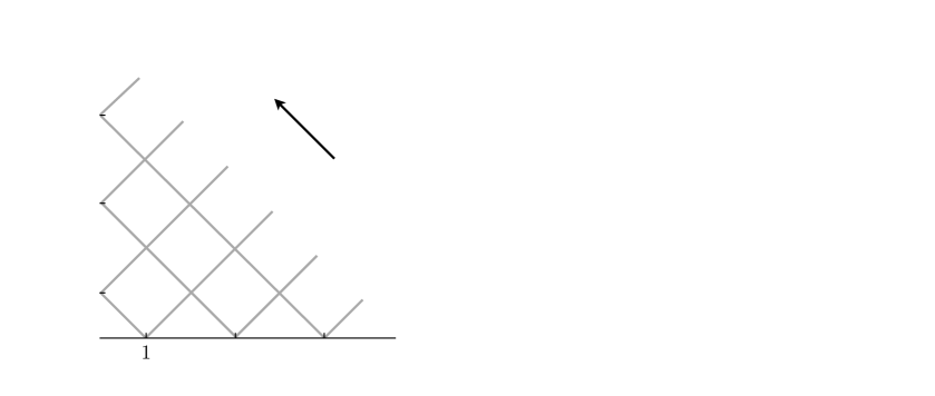
Figure 1: Corner transfer matrix geometries. Left: Gaussian model related to the oscillator chain. Right: Interpenetrating Ising models related to the dimerized hopping chain. Full circles show the location of the dual variables. The arrows indicate the direction of transfer.

In this case, there are explicit expressions for the entanglement Hamiltonians which result from the relation of the chain problem to an integrable two-dimensional lattice model and the use of (infinite-size) corner transfer matrices in the latter. This provides a point of reference for the later treatment of finite subsystems and will therefore be discussed first.

3.1 Harmonic chain

The harmonic chain can be related to a Gaussian model on a square lattice as described in [35]. The necessary CTM was studied before in [34] and is shown in Fig. 1 on the left. This leads to the following expression for the entanglement Hamiltonian of the half chain with sites $i\geq 1$ if one chooses $m=1$, $K=\kappa$ and $\omega=1-\kappa$ in (4)

$$\mathcal{H}_{\textrm{\tiny half}}\,=\,2I(\kappa^{\prime})\sum_{i=1}^{\infty}\frac{1}{2}\Big{[}\,(2i-1)\,p_{i}^{2}+(2i-1)(1-\kappa)^{2}\,q_{i}^{2}+2i\,\kappa\,\big{(}q_{i+1}-q_{i}\big{)}^{2}\,\Big{]}$$ (26)

where $\kappa^{\prime}=\sqrt{1-\kappa^{2}}$ and $I(\kappa)$ is the complete elliptic integral of the first kind which arises from the elliptic parametrisation of the couplings in the Gaussian model.

To get the result in the parametrisation $K=1$ with $\omega$ being independent, one needs to carry out the same canonical transformation employed already for the physical Hamiltonian. In terms of the rescaled variables used in (5) one has

$$\mathcal{H}_{\textrm{\tiny half}}\,=\,2I(\kappa^{\prime})\,\sqrt{\kappa}\sum_{i=1}^{\infty}\frac{1}{2}\Big{[}\,(2i-1)\,\hat{p}_{i}^{2}+(2i-1)\,\omega^{2}\,\hat{q}_{i}^{2}+2i\,\big{(}\hat{q}_{i+1}-\hat{q}_{i}\big{)}^{2}\,\Big{]}$$ (27)

where the rescaled frequency reads

$$\omega^{2}=(1-\kappa)^{2}/\kappa\,.$$ (28)

Note that since $\omega$ is now the free parameter of the Hamiltonian, the relation (28) must be inverted to get the elliptic parameter $\kappa(\omega)$. It is easy to see that the solution is given by (10), such that the elliptic parameter $\kappa$ is identical to the one defining the correlation length.

The operator (27) has thus the same structure as the physical Hamiltonian, but the coefficients of the terms increase linearly as one moves into the subsystem. The matrices $T_{i,j}$ and $V_{i,j}$ introduced in (14) can be read off the expression, and the only non-zero elements are

$$T_{i,i}=b(\kappa)\,(2i-1)\,,\quad V_{i,i}=b(\kappa)\,(2i-1)\,(\omega^{2}+2)\,,\quad V_{i,i+1}=-b(\kappa)\,2i$$ (29)

with $b(\kappa)=2I(\kappa^{\prime})\sqrt{\kappa}$ and $\kappa$ given by (10) in terms of $\omega$.

Finally, the bosonic single-particle eigenvalues $\varepsilon_{l}$ are given by [35]

$$\varepsilon_{l}=\varepsilon\,(2l-1)\,,\quad\quad\varepsilon=\pi\frac{I(\kappa^{\prime})}{I(\kappa)}\,,\quad l=1,2,3,\dots\,.$$ (30)

This result can be checked in the limit $\kappa\rightarrow 0$, where the last term in (26) vanishes and $\mathcal{H}_{\textrm{\tiny half}}$ becomes the sum of independent oscillators multiplied by factors $(2i-1)$.

3.2 Dimerized hopping chain

The entanglement Hamiltonian for this case has not been given before, but it can be obtained from known results for the transverse Ising (TI) chain. The reason is that the dimerized chain is an XX model in spin language which corresponds to two interlacing transverse Ising chains [36, 37, 38, 39]. Consider the two TI Hamiltonians defined on odd resp. even lattice sites

$$\hat{H}_{1} = -\sum_{m}\left(h_{2m-1}\,\sigma^{x}_{2m-1}+\lambda_{2m-1}\sigma^{z}_{2m-1}\sigma^{z}_{2m+1}\right)$$ (31)

$$\hat{H}_{2} = -\sum_{m}\left(h_{2m}\,\sigma^{x}_{2m}+\lambda_{2m}\,\sigma^{z}_{2m}\sigma^{z}_{2m+2}\right)$$ (32)

where $\sigma^{x}_{n},\sigma^{z}_{n}$ are Pauli matrices. Then, going over to dual variables via

$$\sigma^{z}_{m}\sigma^{z}_{m+1}=\tau^{z}_{m}\,,\quad\sigma^{x}_{m}=\tau^{x}_{m-1}\tau^{x}_{m}$$ (33)

the total Hamiltonian $\hat{H}=\hat{H}_{1}+\hat{H}_{2}$ becomes

$$\hat{H}=-\sum_{m}\Big{[}(h_{2m}\tau^{x}_{2m-1}\tau^{x}_{2m}+\lambda_{2m-1}\tau^{z}_{2m-1}\tau^{z}_{2m})+(h_{2m+1}\tau^{x}_{2m}\tau^{x}_{2m+1}+\lambda_{2m}\tau^{z}_{2m}\tau^{z}_{2m+1})\Big{]}.$$ (34)

Therefore one can make the interaction isotropic by choosing

$$h_{2m}=\lambda_{2m-1},\quad h_{2m+1}=\lambda_{2m}$$ (35)

which means that the fields in one chain are the couplings in the other one and vice versa. With a rotation $\tau^{z}\rightarrow\tau^{y}$, the Hamiltonian assumes the form

$$\hat{H}=-\sum_{m}\Big{[}\lambda_{2m-1}(\tau^{x}_{2m-1}\tau^{x}_{2m}+\tau^{y}_{2m-1}\tau^{y}_{2m})+\lambda_{2m}(\tau^{x}_{2m}\tau^{x}_{2m+1}+\tau^{y}_{2m}\tau^{y}_{2m+1})\Big{]}$$ (36)

and describes an inhomogeneous XX chain. The special choice

$$\lambda_{2m-1}=1-\delta\,,\qquad\lambda_{2m}=1+\delta$$ (37)

then leads to the operator (16) if one writes (36) in terms of fermions. The two TI chains involved are homogeneous but with interchanged parameters.

Now, a single TI chain with field $h$ and coupling $\lambda$, is related to an isotropic two-dimensional Ising model on a square lattice with coupling $K$ if $\lambda/h=\mathrm{sh}^{2}(2K)$, and the entanglement Hamiltonian follows from the appropriate CTM as in the bosonic case [8]. The operator $\mathcal{H}_{\textrm{\tiny half}}$ describes again a TI chain and differs somewhat for $\lambda/h<1$ (disordered region) and $\lambda/h>1$ (ordered region), see [40]. In the disordered region, it is

$$\mathcal{H}_{\textrm{\tiny half}}=-\,2I(k^{\prime})\,\frac{1}{2}\,\sum_{i\geq 1}\Big{[}(2i-1)\,\sigma^{x}_{i}+k\,2i\,\sigma^{z}_{i}\sigma^{z}_{i+1}\Big{]}$$ (38)

where $k=\lambda/h$, $k^{\prime}=\sqrt{1-k^{2}}$ and $I(k)$ is the same quantity as before. In the ordered region, $k=h/\lambda$, and $k$ appears in front of the first term in the brackets.

In the present case, one has two interpenetrating Ising lattices, one in the ordered and one in the disordered region. This leads to two interpenetrating CTMs, one with a tip and one without a tip, as shown in Fig. 1 on the right, see also [41]. As a result, the two operators in the exponent satisfy the condition (35) and after the dual transformation one has

$$\mathcal{H}_{\textrm{\tiny half}}=-\,2I(k^{\prime})\,\frac{1}{2}\,\sum_{i\geq 1}\Big{[}\,k\,(2i-1)\,(\tau^{x}_{2i-1}\tau^{x}_{2i}+\tau^{y}_{2i-1}\tau^{y}_{2i})+2i\,(\tau^{x}_{2i}\tau^{x}_{2i+1}+\tau^{y}_{2i}\tau^{y}_{2i+1})\Big{]}$$ (39)

where now, using (37), the parameter $k$ is given by $k=(1-\delta)/(1+\delta)$ as in (22). Writing this in terms of fermions, one arrives at the final result for a half-chain with sites $i\geq 1$

$$\mathcal{H}_{\textrm{\tiny half}}=-\,2I(k^{\prime})\sum_{i\geq 1}\Big{[}\,k\,(2i-1)\,(c_{2i-1}^{\dagger}c_{2i}^{\phantom{{\dagger}}}+\mathrm{h.c.})+2i\,(c_{2i}^{\dagger}c_{2i+1}^{\phantom{{\dagger}}}+\mathrm{h.c.})\Big{]}.$$ (40)

This is a hopping model with hopping amplitudes which increase linearly and, in addition, alternate between 1 and $k$ in exactly the same way as in the physical Hamiltonian (16) (if one divides $\hat{H}$ by $(1+\delta)$). Thus the pattern of strong and weak bonds reappears in the entanglement Hamiltonian, as found in earlier numerical calculations [28]. Note that $\mathcal{H}_{\textrm{\tiny half}}$ in (40) starts with a weak bond between $i=1$ and $i=2$, i.e. the chain is divided at a strong bond. If one wants to consider the opposite situation, the factor $k$ has to be moved to the other term in the bracket.

The fermionic single-particle eigenvalues $\varepsilon_{l}$ of $\mathcal{H}_{\textrm{\tiny half}}$ are given by an expression as for a single TI chain and analogous to the bosonic case

$$\varepsilon_{l}=\varepsilon\,2l\,,\quad\quad\varepsilon=\pi\frac{I(k^{\prime})}{I(k)}\,,\quad l=0,\pm 1,\pm 2,\pm 3,\dots$$ (41)

where the factor $2l$ can be checked by taking the limit $k\rightarrow 0$ in (39) or (40). The pairs $(\varepsilon_{l},\varepsilon_{-l})$ arise from the two TI operators in the original representation and the state with $l=0$ is the analogue of the surface state one finds in the Hamiltonian $\hat{H}$ if the chain is actually cut at the strong bond. For a chain divided at a weak bond, one has to move the factor $k$ as mentioned above, and this changes $2l$ into $2l-1$ in the formula.

4 Interval in the harmonic chain

In this section we consider a finite block made by $N$ consecutive sites in the harmonic chain and calculate the entanglement Hamiltonian numerically from the correlation matrices via (15). As mentioned earlier, we set $m=1$ and $K=1$ in (4) so that only the oscillator frequency $\omega$ remains, from which $\kappa$, related to the correlation length, can be obtained via (10). The numerical data shown in Fig. 2, where $N=200$ and $\omega=1$, have been obtained through a numerical precision given by 800 digits, while for Fig. 3, where $N=100$ and $\omega=10$, we have employed 1000 digits. In general, we have observed that higher precision is required as $N$ or $\omega$ increase.

In Fig. 2 the elements in and near the diagonals of the matrices $T$ and $V$ are shown for $\omega=1$, which corresponds to $\kappa=0.383$ and a correlation length $\xi=1.04$. From previous investigations [19] one expects $\mathcal{H}$ to be extensive, therefore the matrix elements are divided by $N$. Dividing also the site indices by $N$, one finds a perfect collapse of the data for $N=100$ and $N=200$ and thus a well-defined limiting behaviour.

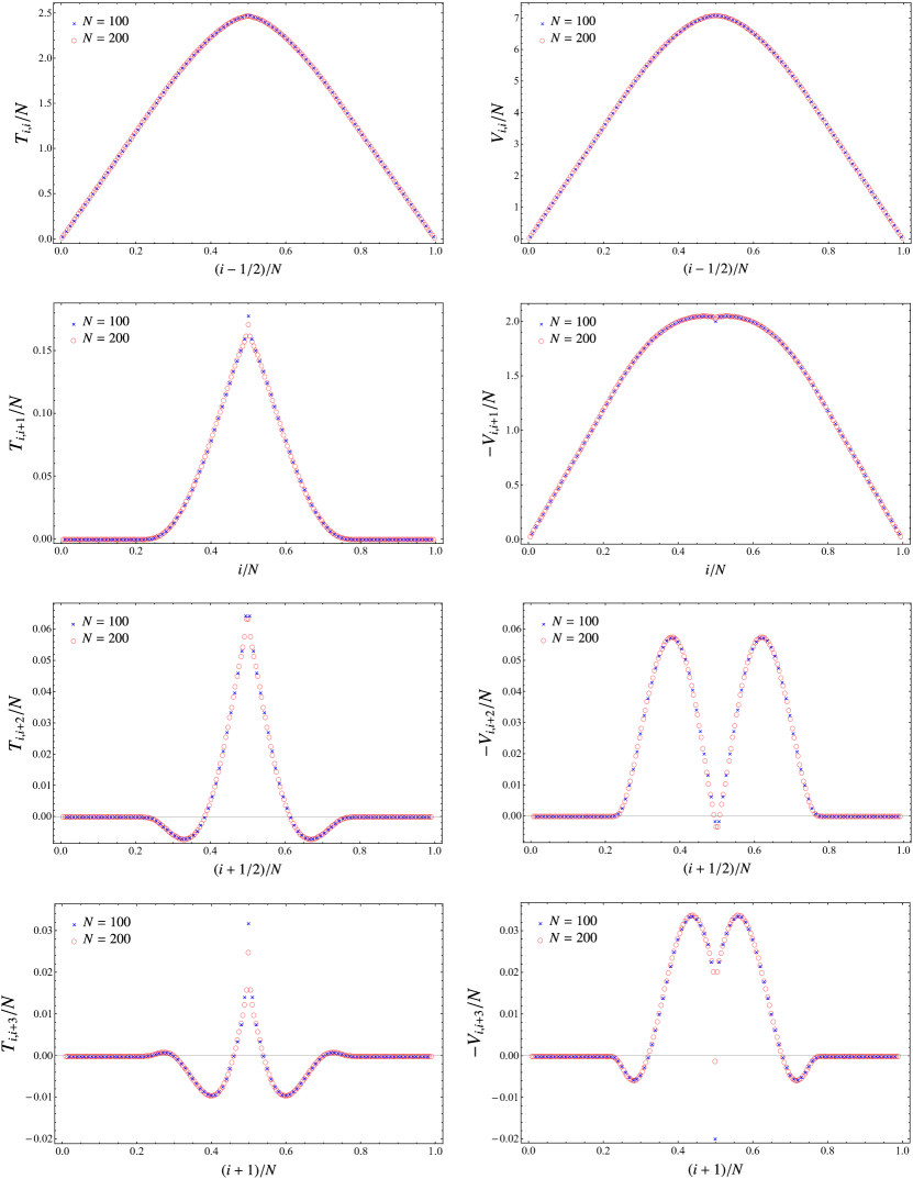
Figure 2: Short-range couplings in the matrices $T$ (left panels) and $V$ (right panels) for $\omega=1$ and two segment sizes. Note the different vertical scales.

In the kinetic energy, only the diagonal elements $T_{i,i}$ are large and show a variation with $i$ which lies somewhere between a parabola and a triangular form. The next elements $T_{i,i+1}$ have a sharp cusp in the middle of the interval and are already an order of magnitude smaller. This cusp remains in the following elements which are still smaller and, in addition, develop more and more structures, including zeros which do not occur in the case of a critical chain [19].

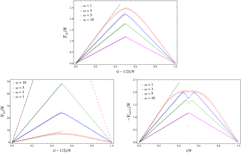
Figure 3: Dominant matrix elements of $T$ and $V$ for $N=100$ and various values of $\omega$. The black dashed lines correspond to the three-diagonals approximation (42) and (43).

In the potential energy, the diagonal elements $V_{i,i}$ are again the largest ones, with a shape similar to that of $T_{i,i}$. However, here the nearest-neighbour terms $V_{i,i+1}$ are also large, negative and show a kind of plateau in the centre. Only the terms describing the interactions with more distant neighbours are much smaller and show structures resembling those in the kinetic terms. Note that we have plotted $-V_{i,i+r}$ for $r>0$. These are the spring constants if one rewrites the potential energy properly and therefore typically positive.

A particular feature is that the structures in the small matrix elements only appear in a certain region in the centre of the subsystem, while the quantities are zero in the rest of the interval. This region is the same for all quantities and its width becomes smaller and approaches zero as $\omega$ increases, i.e. as the coupling between the oscillators in the chain becomes less important (see also Fig. 10).

In Fig. 3 we look at the three dominant matrix elements $T_{i,i}$, $V_{i,i}$ and $V_{i,i+1}$ in more detail. They are shown there for relatively large values of $\omega$, ranging from $\omega=1$ ($\kappa=0.38$, $\xi=1$) to $\omega=10$ ($\kappa=0.01$, $\xi=0.2$) and one sees that all approach a triangular shape as $\omega$ increases. The dashed lines are the slopes found in (29) for the half-infinite subsystem and describe the results very well. This suggests an approximation which consists in keeping only these elements and setting

$$\frac{T_{i,i}}{N}=2\,b(\kappa)\,\Delta((i-1/2)/N)$$ (42)

and

$$\frac{V_{i,i}}{N}=2\big{(}\omega^{2}+2\big{)}\,b(\kappa)\,\Delta((i-1/2)/N)\,,\;\qquad\;\frac{V_{i,i+1}}{N}=-\,2\,b(\kappa)\,\Delta(i/N)$$ (43)

with the “triangular” function

$$\Delta(x)\equiv\frac{1}{2}-\left|\,x-\frac{1}{2}\,\right|=\Bigg{\{}\begin{array}[]{ll}x&0\leq x\leq 1/2\\ 1-x&1/2\leq x\leq 1\\ \end{array}$$ (44)

replacing the simple linear behaviour in (29). In physical terms, this three-diagonals approximation models the entanglement Hamiltonian $\mathcal{H}$ of the interval by glueing the half-infinite ones attached to the endpoints together. This should be good for small correlation lengths and the analytical expressions allow to predict how the slopes vary with $\omega$. Since $\kappa$ decreases as $\omega$ becomes larger, $b(\kappa)$ also decreases while $\omega^{2}\,b(\kappa)$ increases.

While this approximation describes $\mathcal{H}$ quite well, it neglects the structure in the nearest-neighbour coupling $V_{i,i+1}$ in the middle of the subsystem. This probably has to be seen together with the features in the small longer-distance couplings.

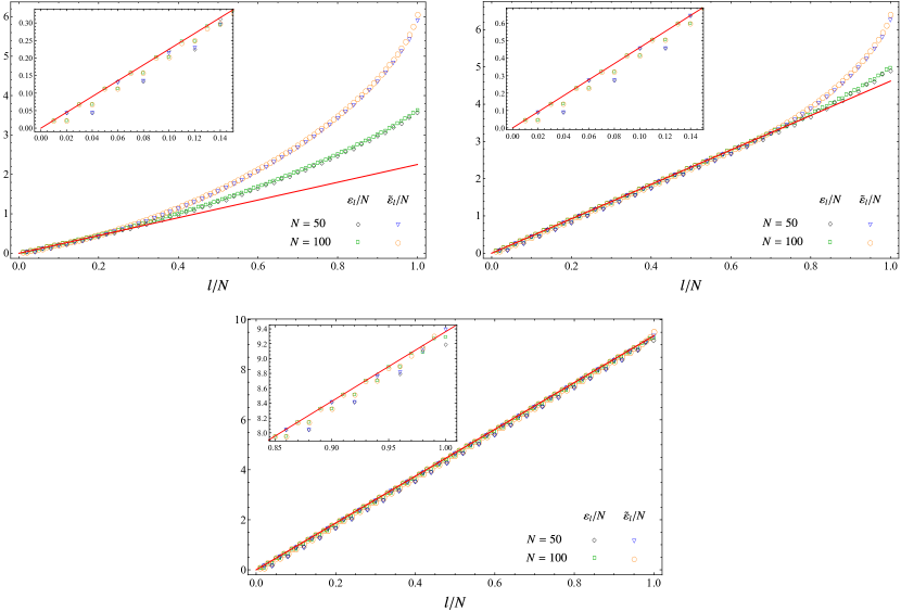
Figure 4: Exact and approximate single-particle entanglement eigenvalues $\varepsilon_{l}$ and $\tilde{\varepsilon}_{l}$ for $\omega=0.1$ (top left), $\omega=1$ (top right) and $\omega=5$ (bottom). The slope of the red solid line is given by $\varepsilon$ in (30).

Finally, we turn to the single-particle spectra $\varepsilon_{l}$ which follow from the eigenvalues of the matrix $PQ$ according to (13). They are shown in Fig. 4 for three typical values of $\omega$. As $\mathcal{H}$ scales with $N$, so do the $\varepsilon_{l}$, and a plot $\varepsilon_{l}/N$ vs. $l/N$ gives a universal curve for large $N$. Basically, the $\varepsilon_{l}$ increase at first linearly with $l$, but for large $l$ there is an upward bend. This sets in early for small $\omega$ and late for larger $\omega$. Already for $\omega=5$ the behaviour is just linear. The full lines are the results of (30) and are seen to describe the (initial) slope very well. A closer look at the smaller eigenvalues for $\omega=0.1$ and $\omega=1$ is provided by the insets and shows that they are doubly degenerate, as one would expect if one associates them with the two boundaries. The degenerate levels are described by the half-chain formula (30). As the dispersion bends, the degeneracy is also lost.

In Fig. 4 the eigenvalues $\tilde{\varepsilon}_{l}$ result from the entanglement Hamiltonian based on the three-diagonals approximation (42) and (43). For large $\omega$, a perfect agreement between the two sets is observed up to the largest few eigenvalues, as shown in the inset for $\omega=5$. In contrast, for smaller values of $\omega$ the $\tilde{\varepsilon}_{l}$ lie above the $\varepsilon_{l}$ at the upper end of the spectrum. This is quite reasonable since the triangular form in (42) and (43) overestimates the largest matrix elements in the middle of the interval which mainly determine the largest eigenvalues, since the eigenfunctions are concentrated there. By contrast, there is always agreement between $\tilde{\varepsilon}_{l}$ and $\varepsilon_{l}$ at the lower end.

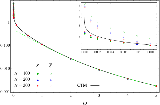
Figure 5: Entanglement entropy as function of $\omega$: $S$ is obtained through the exact formula (45), $\widetilde{S}$ through the three-diagonals approximation and the solid black curve corresponds to (46). The green dashed line shows the approximation (60) for $\omega\gg 1$, while the inset shows the behaviour for $\omega\ll 1$.

With the eigenvalues $\varepsilon_{l}$, the entanglement entropy is given by

$$S=\sum_{l=1}^{N}\left(\frac{\varepsilon_{l}}{e^{\varepsilon_{l}}-1}-\ln\,(1-e^{-\varepsilon_{l}})\right)$$ (45)

and the result of the numerical calculation is shown in Fig. 5 where $S$ is plotted as a function of $\omega$. For $\omega>1$ one can safely use the spectrum of the half-infinite subsystem given in (30) plus the two-fold degeneracy. Following the steps sketched in appendix A, a closed formula for the entropy can be found as

$$S=-\frac{1}{12}\left[\ln\left(\frac{16\kappa^{\prime 4}}{\kappa^{2}}\right)-(1+\kappa^{2})\frac{4I(\kappa)I(\kappa^{\prime})}{\pi}\right].$$ (46)

It differs by a factor $2$ from the one reported in [2] for the half-infinite chain, reflecting the contributions from the two endpoints of the interval. The result (46) is shown by the solid black line in Fig. 5, which perfectly agrees with the numerical data.

This agreement actually extends to much smaller $\omega$ as shown in the inset, where deviations occur only below $\omega=0.01$ (corresponding to correlation length $\xi=100$). The same holds for the entropy $\widetilde{S}$ calculated with the eigenvalues $\tilde{\varepsilon}_{l}$, because $S$ is determined essentially by the low end of the spectrum.

5 Interval in the dimerized chain

The study of the dimerized hopping chain is somewhat simpler as one has only the matrix $H$ to consider. The corresponding matrix elements are given by (25) via the eigenvalue equation (23) of the reduced correlation matrix. Similarly to the bosonic case, this requires the matrix elements of $C$ to be calculated with a high precision via the analytic expressions in (19)-(21). Due to the particle-hole symmetry, the nonvanishing entries $H_{i,j}$ are hopping terms over an odd distance $|j-i|=2p+1$ and it is useful to define their density as

$$h_{i,j}=-\frac{H_{i,j}}{N}\,.$$ (47)

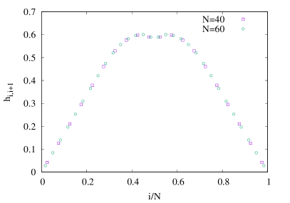
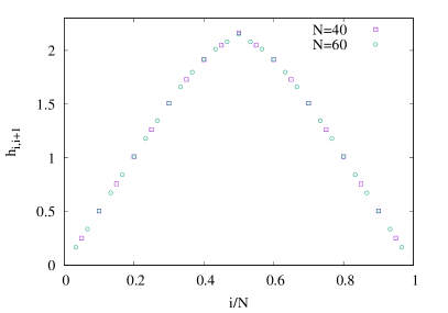
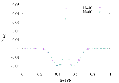
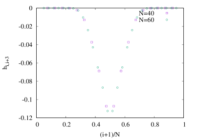
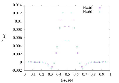
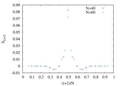
Figure 6: First-, third- and fifth-neighbour hopping in $H$ for odd (left) and even (right) bonds, with dimerization $\delta=0.5$ and for two segment sizes. Note the different vertical scales.

To get an overall impression on the structure of the entanglement Hamiltonian, in Fig. 6 we plot the scaled hopping amplitudes in (47) along the diagonals up to the fifth-neighbour terms, for a dimerization parameter $\delta=0.5$. The hopping amplitudes $h_{i,i+2p+1}$ depend on the scaling variable $(i+p)/N$ as is clear from the data collapse for two different segment sizes. The hopping matrix is dominated by the nearest-neighbour terms ($p=0$), similarly to the homogeneous chain $(\delta=0)$. However, the dimerization induces a strong variation of the hopping across even and odd bonds, shown by the left and right columns in Fig. 6. The third- and fifth-neighbour hopping ($p=1,2$) is an order of magnitude smaller and has a nontrivial structure, developing sharp peaks in the center, which is reminiscent of the behaviour seen for the oscillator chain in Fig. 2. Note also that, in contrast to the homogeneous case where $h_{i,i+2p+1}>0$ for all $p$, the amplitudes $h_{i,i+3}$ are dominantly negative for the dimerized case. We checked numerically that this sign change occurs gradually as one moves towards $\delta\to 0$.

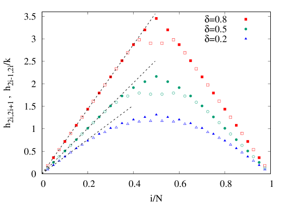
Figure 7: Nearest-neighbour hopping in the entanglement Hamiltonian of the dimerized chain for various $\delta$ and $N=40$. The hopping across odd bonds (empty symbols) is divided by a factor of $k$. The dashed lines have slopes $2I(k^{\prime})$ corresponding to the result for the half-infinite subsystem in (40).

We shall now focus on the nearest-neighbour hopping and use the exact results for the half-infinite chain in Sec. 3 to obtain an approximate understanding for the segment. Our main physical argument is that in a non-critical system with correlation length $\xi\ll N$, the segment should effectively behave like a half-infinite system around both of its boundaries. Hence, the result in Eq. (40) predicts a linear increase of the hopping with a slope $2I(k^{\prime})$, multiplied by a factor of $1$ or $k$ for the strong (even) and weak (odd) bonds. To check this prediction, we have plotted in Fig. 7 the hopping profiles $h_{2i,2i+1}$ and $h_{2i-1,2i}/k$, and compared them to the half-infinite result shown by the dashed lines. The linear approximation works perfectly around the boundary of the segment, with the agreement improving towards the center for larger $\delta$. One should remark that all the $\delta$ values in Fig. 7 correspond to very short correlation lengths, in particular one has $\xi\approx 2.5$ for $\delta=0.2$. Nevertheless, the deviation from the wedge profile for this value is more pronounced. Clearly, in the limit $\delta\to 0$ one has to recover the result for the critical case [16], which is roughly parabolic with a slope $2I(0)=\pi$ at the boundaries. Note also that the odd hopping profile develops a dip around the center, in contrast to the even profile which has a marked peak.

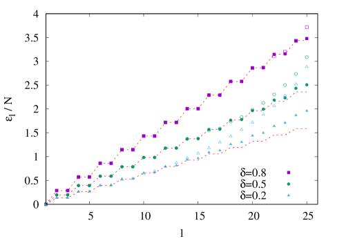
Figure 8: Comparison of the scaled single-particle entanglement spectra $\varepsilon_{l}/N$ (full symbols) to those $\tilde{\varepsilon}_{l}/N$ (empty symbols) calculated from $\tilde{h}$ for $N=50$ and various $\delta$. The dashed red lines show the half-infinite result in Eq. (41) with double degeneracy. Only positive eigenvalues are shown.

Despite the systematic deviations, one expects that a simple nearest-neighbour entanglement Hamiltonian $\tilde{h}_{i,j}$ with wedge-like hopping amplitudes would give a very good approximation $\tilde{\rho}$ of the actual reduced density matrix $\rho$. In fact, in the critical case $\delta=0$, it has recently been shown that such an approximation with a parabolic hopping profile yields a vanishing distance between $\tilde{\rho}$ and $\rho$ as $N\to\infty$ [27]. For the dimerized chain we assume, analogously to the oscillator chain in (42) and (43), a triangular profile for the nearest-neighbour hopping

$$\tilde{h}_{2i-1,2i}=2I(k^{\prime})\,k\,\Delta((2i-1)/N)\,,\;\;\qquad\;\;\tilde{h}_{2i,2i+1}=2I(k^{\prime})\,\Delta(2i/N)$$ (48)

where the function $\Delta(x)$ was defined in (44), and we set $\tilde{h}_{i,i+2p+1}=0$ for all $i$ and $p>0$. To check the feasibility of such an approximation, in Fig. 8 we compare the spectra $\tilde{\varepsilon}_{l}$ calculated from $\tilde{h}$ to the actual spectrum $\varepsilon_{l}$, studied previously in Ref. [42]. Note that due to particle-hole symmetry, the eigenvalues come in pairs with opposite signs, and we show only the positive part of the spectra for better visibility. Clearly, the low-lying part of the spectrum is perfectly reproduced, while the larger eigenvalues $\varepsilon_{l}$ tend to be overestimated by $\tilde{\varepsilon}_{l}$. The agreement of the high-energy spectrum improves for larger dimerizations, and for $\delta=0.8$ it already becomes perfect up to the last few eigenvalues. Note also that the low-lying spectra are doubly degenerate, corresponding to contributions from the two boundaries, and the levels are given by the CTM result (41) for the half-infinite chain, shown by the dashed lines in Fig. 8. The observed features are completely analogous to those shown in Fig. 4 for the oscillator chain.

It is instructive to have a look also at the entanglement entropy, given by

$$S=\sum_{l=1}^{N}\left(\frac{\varepsilon_{l}}{e^{\varepsilon_{l}}+1}+\ln\,(1+e^{-\varepsilon_{l}})\right).$$ (49)

The quantity $\tilde{S}$ calculated via $\tilde{\varepsilon}_{l}$ is defined analogously. As only the low-lying $\varepsilon_{l}$ have a significant contribution, it is already clear from Fig. 8 that $\tilde{S}$ would give a perfect approximation of the entropy for the $\delta$ values shown. Therefore we now focus on smaller dimerizations $|\delta|<0.1$, corresponding to larger correlation lengths, with the results for $N=50$ shown in Fig. 9. Remarkably, the agreement between $S$ and $\tilde{S}$ remains very good down to $|\delta|\approx 0.025$ corresponding to $\xi\approx 20$. For even smaller $|\delta|$ the correlation length exceeds the half-length of the segment, and the ansatz (48) built from the contributions of two independent boundaries gradually breaks down. The same is true for the doubled CTM result which, using the formulas for the TI chain [43, 2], can be written as

$$S=\begin{cases}\displaystyle\;\frac{1}{3}\left[\ln\Big{(}\frac{k^{2}}{16k^{\prime}}\Big{)}+\Big{(}1-\frac{k^{2}}{2}\Big{)}\frac{4I(k)I(k^{\prime})}{\pi}\right]+2\ln 2\;\;\;&\delta>0\\ \rule{0.0pt}{28.45274pt}\displaystyle\;\frac{1}{6}\left[\ln\Big{(}\frac{16}{k^{2}k^{\prime 2}}\Big{)}+(k^{2}-k^{\prime 2})\frac{4I(k)I(k^{\prime})}{\pi}\right]&\delta<0\end{cases}$$ (50)

where for $\delta<0$ one has to use $|\delta|$ in the definition (22) such that $k<1$. In particular, for $\delta\to 0$ ($k\to 1$) the CTM result diverges logarithmically. In contrast, the entropy $\tilde{S}$ was found to scale as $\tilde{S}=1/3\ln N+\mathrm{const}$, reproducing the correct prefactor but not the proper constant in $S$. Although the correct ansatz for the hopping is a parabola for $\delta=0$, the triangular profile has the same slope at the boundaries and thus reproduces the proper logarithmic scaling of the entropy.

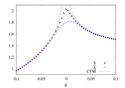
Figure 9: Entanglement entropy $S$ and its approximation $\tilde{S}$ as a function of the dimerization strength for $N=50$. The red dashed lines show the CTM result in Eq. (50).

6 General features of the non-critical regime

Figure 10: Contour plots of $T_{i,j}/N$ (top) and $V_{i,j}/N$ (bottom) for $N=400$ and six values of $\omega$.

In the last two sections, we focussed on strongly non-critical systems with a correlation length of the order of the lattice constant and thus much smaller than the length of the interval. Here we want to outline the situation in the whole non-critical region.

For the dominant matrix elements, this was done to some extent already in Figs. 2 and 3 (see Figs. 6 and 7 for the fermionic chain), where a transition from parabolic to triangular profiles could be observed as $\xi$ became smaller. The properties of all others are collected in the form of contour plots in Fig. 10 for the case of the oscillator chain, where the elements $T_{i,j}/N$ and $V_{i,j}/N$ for $N=400$ and six different values of $\omega$ are shown. The size of the elements is given by a colour code where white represents values smaller than $10^{-5}$. The case $\omega=10^{-30}$ corresponds to a system which is essentially critical and this was studied in detail in [19]. The finite value of $\omega$ only serves to avoid a zero mode in the chain. The cases $\omega=1$ and $\omega=3$ correspond to the situation considered in section 4. One sees that in both limits the matrices have somewhat larger elements only near the main diagonal. Physically, these are short-range couplings. As one moves away from criticality, larger regions of the squares become filled (in particular for $T_{i,j}$), a cross-shaped structure develops in the middle and then shrinks again. Calculations for larger $\omega$ show that it vanishes around $\omega=100$. Its finite extent in the direction of the main diagonal was already encountered in Fig. 2, where the matrix elements $V_{i,i+r}$ for small $r$ were seen to vanish beyond a certain distance from the centre. The elements in the other arm of the cross correspond to longer-range couplings near and across the centre, and a particular case is the sharp “antidiagonal” in the matrix of the potential energy, formed by the elements $V_{i,N+1-i}$ which connect points symmetric with respect to the middle of the interval. In particular $i=1$ corresponds to a coupling across the whole subsystem. This structure was already observed in [17].

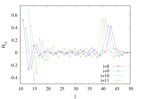
Figure 11: Hopping amplitudes $H_{i,j}$ along a fixed row $i$ in the dimerized chain. The data are shown for $N=50$ as a function of $j>i+1$, omitting the dominant nearest-neighbour term.

For the dimerized hopping model, an analogous plot of $H_{i,j}/N$ shows similar features and resembles the picture for $\omega=10^{-2}$ in Fig. 10. The structure is always cross-like and a sharp antidiagonal exists. In Fig. 11 we present this feature in more detail by showing horizontal cuts through the matrix, plotting the elements $H_{i,j}$ for fixed $i$ as function of the column index $j$. One sees not only a sharp spike right at $j=N+1-i$, but already an increase of the values as the antidiagonal is approached while they are initially decreasing with $j$. This behaviour can also be inferred from the contour plots, but is clearer in the direct plot. As to the values along the antidiagonal, these are shown in Fig. 12 for several dimerizations $\delta$. While close to criticality, they are small and decrease only slowly with $i$, they become larger in the centre for stronger dimerization but also decrease faster, approaching zero at some finite point. Remarkably, plotted against $i/N$ and away from the centre, the amplitudes $H_{i,N+1-i}$ along the antidiagonal collapse on the same curve for various $N$ and are thus nonextensive, in sharp contrast to the short-range hopping in Fig. 6. This is similar to the situation for the central structure in the oscillator chain. In that case, one finds a similar profile along the antidiagonals, but the alternations of the dimerized chain are absent.

The phenomenon of the antidiagonals is somewhat intriguing but does not seem to have a simple interpretation. In [17] it was shown to arise in a perturbative calculation around the critical point, where it comes from the logarithmic oscillations of the critical eigenfunctions, but this is more a formal argument.

Altogether these results show that the structure of the matrices, as far as the small entries are concerned, is most complex in the transition region where $\xi\sim N$. This is not unexpected, since there the effects from both ends of the interval start to mix, but it will be seen below to cause problems in a continuum limit.

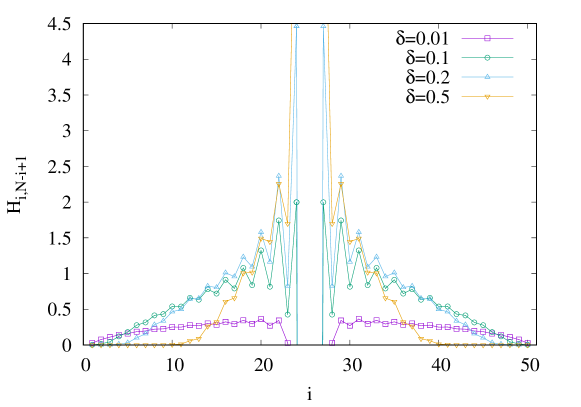
Figure 12: Hopping amplitudes $H_{i,N-i+1}$ along the antidiagonal for $N=50$ and various $\delta$, omitting the dominant nearest-neighbour terms in the middle.

7 Summary and discussion

We have determined the entanglement Hamiltonian of an interval in a non-critical chain for two systems which allow for an explicit calculation, one bosonic and one fermionic. In both cases, one had to resort to numerics, but the analytical results for the infinite interval provided a strong guidance. Quite generally, the matrices describing the quadratic Hamiltonian $\mathcal{H}$ in real space contain couplings over arbitrary distances. However, as in the critical cases studied before, only those with short range are large, whereas all others are significantly smaller. In this sense, the situation is simple, and an obvious approximate treatment consists in keeping only the large elements. Using in addition the analytical results for them then leads to a Hamiltonian with a triangular variation of the terms along the interval. This was seen to reproduce the low-lying single-particle eigenvalues very accurately over most of the parameter space. As a consequence, also the resulting entanglement entropies are correct except in a small region around the critical point. This is a variant of the “corner Hamiltonian” approach [44, 45] in which one replaces the true entanglement Hamiltonian by one with linearly varying couplings.

All our considerations were for lattice systems, but one can ask about a possible continuum limit in the vicinity of the critical point, by introducing a lattice spacing $a$ and taking $a\to 0$. In fact, for the half-infinite interval this limit can easily be taken and leads to the Bisognano-Wichmann result (1). This is outlined in Appendix B for the oscillator chain. For the finite interval, one knows that the small longer-range couplings on the lattice should be included properly. This leads to sums along horizontal cuts of the corresponding matrices. For example, the mass parameter $m(x)$ in the continuum description, with $x=ia$, is given in the oscillator chain by

$$m(x)=\sum_{r}V_{i,i+r}$$ (51)

whereas the local velocity is

$$v(x)=\sum_{r}r^{2}\,V_{i,i+r}$$ (52)

and a similar expression holds for the local Fermi velocity $v_{F}(x)$ in the dimerized chain. It turns out that, in contrast to the situation at criticality, one may need a large number of terms in order to obtain convergence of the sums, for example 30 terms for $v_{F}(x)$ if $\delta=0.05$ and $N=100$. Then $v_{F}(x)$ shows a triangular profile, but the better converging $m(x)$ looks roughly parabolic with an additional structure in the centre. However, further increasing the cutoff in the sums, the numerical results for the velocity and mass parameter become unstable, and even more severe irregularities tend to occur also for the oscillators. Here, the particular features of the matrices including the antidiagonals enter. Altogether, we were not able to obtain well-defined general results in the massive regime by fixing $N/\xi$ and increasing $N$. This hints toward the possibility that the naive continuum limit, that perfectly reproduces the CFT results in the massless case [18, 19], might not be valid away from criticality and that $\mathcal{H}$ remains non-local also in the continuum [17].

A closely related question is, whether a commuting operator with short-range couplings exists in these non-critical chains. The simple ansatz in Appendix C was not totally successful, but it could be that more general forms like in [46] do work. That would be an important step and would shed additional light on the problem considered here.

Appendix A Half-infinite subsystem: bosonic entanglement entropy

In this appendix we indicate the steps for obtaining a closed formula for the entanglement entropy if the single-particle eigenvalues $\varepsilon_{l}$ of $\mathcal{H}$ are given by the CTM result (30) in section 3. The expression (45) follows from the general formula

$$S=\ln Z+U$$ (53)

with the partition function $Z$ and the internal energy $U$. These are given by

$$1/Z=\prod_{l}(1-e^{-\varepsilon_{l}})=\prod_{{l}=1}^{\infty}(1-q^{2{l}-1})$$ (54)

$$U=\sum_{l}\frac{\varepsilon_{l}}{e^{\varepsilon_{l}}-1}=\varepsilon\sum_{{l}=1}^{\infty}(2{l}-1)\frac{q^{2{l}-1}}{1-q^{2{l}-1}}$$ (55)

where $q=\exp(-\pi I(\kappa^{\prime})/I(\kappa))$.

The product in (54) can be obtained from formula (16.37.4) in [47] for the Jacobi theta function $\vartheta_{n}(u)$ by putting $m=\kappa^{2},m_{1}=\kappa^{\prime 2},u=0$ and using $\vartheta_{n}(0)=1$. This gives

$$\prod_{{l}=1}^{\infty}(1-q^{2{l}-1})=\left(\frac{16q\kappa^{\prime 4}}{\kappa^{2}}\right)^{1/24}.$$ (56)

The sum in (55) can be obtained from from formula (16.23.10) in [47] for the function ns(u) which reads, correcting a sign,

$$\mathrm{ns}(u)=\frac{\pi}{2I}\mathrm{csc}(v)+\frac{2\pi}{I}\sum_{{l}=1}^{\infty}\frac{q^{2{l}-1}}{1-q^{2{l}-1}}\sin((2l-1)v)\,,\quad v=\frac{\pi u}{2I}\,,\quad I=I(\kappa)\,.$$ (57)

Expanding the functions $\mathrm{ns}(u)=1/\mathrm{sn}(u)$ and $\mathrm{csc}(v)=1/\sin(v)$ for small $u$ and small $v$ respectively, the leading terms proportional to $1/u$ cancel and the coefficients of $u$ give the result

$$\sum_{l=1}^{\infty}(2{l}-1)\frac{q^{2{l}-1}}{1-q^{2{l}-1}}=-\frac{1}{24}\left[1-(1+\kappa^{2})\left(\frac{2I}{\pi}\right)^{2}\right].$$ (58)

Taking these results together, one finds for the entropy the formula reported in [2].

For a comparison with the case of an interval, $S$ should be multiplied by $2$ due to degeneracy of the eigenvalues $\varepsilon_{l}$, which leads to the result (46). For $\kappa\rightarrow 1$, i.e. near criticality, the entropy (46) diverges and, using $I(\kappa)\simeq\ln(4/\kappa^{\prime})$, one has for the interval

$$S\simeq\frac{1}{3}\ln\left(\frac{1}{1-\kappa}\right)$$ (59)

while for $\kappa\rightarrow 0$ it goes to zero as

$$S\simeq\frac{1}{4}\,\kappa^{2}(-\ln\kappa+1/2+\ln 4)$$ (60)

because the coupling of the oscillators vanishes. The expression (60) in the regime $\omega\gg 1$, that corresponds to $\kappa\to 0$ from (10), is shown by the green dashed line in Fig. 5.

Appendix B Half-infinite subsystem: continuum limit

For a half-infinite interval, the entanglement Hamiltonians in both models have the same structure as the corresponding chain Hamiltonians. Taking a continuum limit therefore involves the same steps in both quantities and is rather straightforward. We sketch it here for the oscillator chain.

In place of the discrete variables $\hat{q}_{n}$ and $\hat{p}_{n}$, fields $\Phi(x)$ and $\Pi(x)$ are introduced via

$$\hat{q}_{n}\,\longrightarrow\,\Phi(x)\,,\;\;\qquad\;\;\hat{p}_{n}\,\longrightarrow\,a\,\Pi(x)$$ (61)

where $x=n\,a$ and $a\to 0$ denotes the lattice constant. Correspondingly, $\Pi(x)$ is a momentum per length. Replacing also sums by integrals according to $a\sum_{n}\to\int dx$ and differences of $\hat{q}_{n}$ by first derivatives, the Hamiltonian (5) becomes

$$\hat{H}=a\,\sqrt{K/m}\int_{-\infty}^{\infty}dx\;\frac{1}{2}\left[\,\Pi(x)^{2}+\big{(}\Phi^{\prime}(x)\big{)}^{2}+\Omega^{2}\,\Phi(x)^{2}\,\right]\,.$$ (62)

Here $\Omega$, which is the mass parameter in the field theory, is given by

$$\Omega\equiv\frac{\omega}{a\,\sqrt{K/m}}$$ (63)

and we recall that $K=m=1$ in our numerical calculations. One sees that, if $\Omega$ has to remain finite for $a\to 0$, also $\omega$ has to vanish in this limit. The Hamiltonian (62) provides the following expression for the energy density in the continuum theory

$$\mathcal{T}_{00}(x)\,\equiv\,\frac{1}{2}\left[\,\Pi(x)^{2}+\big{(}\Phi^{\prime}(x)\big{)}^{2}+\Omega^{2}\,\Phi(x)^{2}\,\right].$$ (64)

In the same way, the entanglement Hamiltonian (27) becomes

$$\mathcal{H}_{\textrm{\tiny half}}\,=\,2I(\kappa^{\prime})\,\sqrt{\kappa}\int_{0}^{\infty}dx\;\frac{1}{2}\Big{[}\,2x\,\Pi^{2}+2x\,\Omega^{2}\,\Phi^{2}+2x\,(\Phi^{\prime})^{2}\,\Big{]}$$ (65)

where the factors of $2x$ arise from $(2i-1)a$ and $2ia$, respectively. This can be written in terms of the energy density (64) as

$$\mathcal{H}_{\textrm{\tiny half}}\,=\,2b(\kappa)\int_{0}^{\infty}dx\,x\,\mathcal{T}_{00}(x)\,,\;\;\qquad\;\;b(\kappa)\equiv 2I(\kappa^{\prime})\,\sqrt{\kappa}\,.$$ (66)

Here the coefficient $b(\kappa)$ depends on $\omega$ if one uses $\kappa(\omega)$ from (10). According to the remark above, $\omega\to 0$ in the continuum limit, which gives $\kappa\to 1$ and $\kappa^{\prime}\to 0$, thus $I(\kappa^{\prime})\to\pi/2$ and one ends up with $2b(\kappa)\to 2\pi$, which is the value predicted by the Bisognano-Wichmann theorem [5, 6].

Appendix C Quasi-commuting tridiagonal matrix

A remarkable feature of the homogeneous hopping chain is the existence of a tridiagonal matrix that exactly commutes with the matrix $H$ in the entanglement Hamiltonian [48, 49]. For an infinite chain the hopping profile is exactly parabolic, but generalizations to a finite ring [50] or an open chain [51] also exist. Some nontrivial examples of inhomogeneous hopping chains were recently also uncovered using the theory of bispectrality [52, 53]. Motivated by these examples and the results in section 5, a natural guess of a commuting tridiagonal matrix for the dimerized chain could be given by

$$T=\left(\begin{array}[]{ccccc}0&t_{1}&&&\\ t_{1}&0&t_{2}&&\\ &t_{2}&0&t_{3}&\\ &&\ddots&\ddots&\\ &&&t_{N-1}&0\end{array}\right)$$ (67)

with triangular hopping

$$t_{2i-1}=(1-\delta)\,\Delta\Big{(}\frac{2i-1}{N}\Big{)},\qquad t_{2i}=(1+\delta)\,\Delta\Big{(}\frac{2i}{N}\Big{)}$$ (68)

where the function $\Delta(x)$ was defined in (44).

In the following we shall show that, although the matrix $T$ does not exactly commute with $C$ (and hence with $H$), the matrix elements of the commutator $\left[C,T\right]_{i,j}$ are identically zero for $i,j\leq N/2$ and $i,j>N/2$. Indeed, one has

$$\left[C,T\right]_{i,j}=C_{i,j-1}t_{j-1}-C_{i+1,j}t_{i}+C_{i,j+1}t_{j}-C_{i-1,j}t_{i-1}$$ (69)

with the boundary conditions $t_{0}=t_{N}=0$. Due to the checkerboard structure of $C$, we only have to consider the cases $i=2m$ and $j=2n$ or $i=2m-1$ and $j=2n-1$. Setting $r=2m-2n-1$ and using the definitions (18), one has for $i,j\leq N/2$

$$-N\left[C,T\right]_{2m,2n}=\, \left[(r+2)\,\mathcal{C}_{r+2}+r\,\mathcal{C}_{r}\right]+\delta^{2}\left[(r+2)\,\mathcal{S}_{r+2}-r\,\mathcal{S}_{r}\right]$$

$$+(2m+2n-1)\,\delta\left[\mathcal{C}_{r+2}-\mathcal{C}_{r}+\mathcal{S}_{r+2}+\mathcal{S}_{r}\right].$$ (70)

Let us first prove that the second line gives zero, i.e. the expression in the brackets vanishes. This can be proved easily by using only trigonometric identities. For the piece $\mathcal{C}_{r+2}-\mathcal{C}_{r}$ the trigonometric expression in the numerator of the integrand becomes

$$(-2\sin^{2}q\cos qr-\sin qr\sin 2q)\cos q$$ (71)

whereas for $\mathcal{S}_{r+2}+\mathcal{S}_{r}$ one has

$$(2\cos^{2}q\sin qr+\sin 2q\cos qr)\sin q\,.$$ (72)

One can trivially show that the sum of the two pieces gives zero.

It is more complicated to prove that the first line of (70) also vanishes. Let us rewrite

$$(r+2)\,\mathcal{C}_{r+2}+r\,\mathcal{C}_{r}=\int_{-\pi/2}^{\pi/2}\frac{dq}{2\pi}\frac{\cos q}{\sqrt{\cos^{2}q+\delta^{2}\sin^{2}q}}\frac{d}{dq}(\sin q(r+2)+\sin qr)$$ (73)

$$(r+2)\,\mathcal{S}_{r+2}-r\,\mathcal{S}_{r}=\int_{-\pi/2}^{\pi/2}\frac{dq}{2\pi}\frac{\sin q}{\sqrt{\cos^{2}q+\delta^{2}\sin^{2}q}}\frac{d}{dq}(-\cos q(r+2)+\cos qr)$$ (74)

and integrate by parts. Using

$$\frac{d}{dq}\frac{\cos q}{\sqrt{\cos^{2}q+\delta^{2}\sin^{2}q}}=\frac{-\delta^{2}\sin q}{(\cos^{2}q+\delta^{2}\sin^{2}q)^{3/2}}$$ (75)

$$\frac{d}{dq}\frac{\sin q}{\sqrt{\cos^{2}q+\delta^{2}\sin^{2}q}}=\frac{\cos q}{(\cos^{2}q+\delta^{2}\sin^{2}q)^{3/2}}$$ (76)

one can rewrite the term in the first line of (70) as

$$\delta^{2}\int_{-\pi/2}^{\pi/2}\frac{dq}{2\pi}\frac{(\sin q(r+2)+\sin qr)\sin q+(\cos q(r+2)-\cos qr)\cos q}{(\cos^{2}q+\delta^{2}\sin^{2}q)^{3/2}}\,.$$ (77)

Note that the numerator in this integrand is now exactly the same trigonometric expression that has been shown to vanish above. Finally, it is also easy to check that the boundary terms from the integration by parts vanish as well for arbitrary odd $r$.

The calculations for $i=2m-1$ and $j=2n-1$ as well as for the case $i,j>N/2$ follow similarly. Unfortunately, however, the absolute value in the expression of the triangular function $\Delta(x)$ spoils the commutation property if the indices $i$ and $j$ are taken in different halves of the segment. Nevertheless, for large dimerizations the nonvanishing matrix elements of the commutator in (69) are very small, as the elements of $C$ decay exponentially with the distance from the diagonal.

References

References

- [1] Calabrese P, Cardy J and Doyon B 2009 Entanglement entropy in extended quantum systems J. Phys. A: Math. Theor. 42 500301
- [2] Peschel I and Eisler V 2009 Reduced density matrices and entanglement entropy in free lattice models J. Phys. A: Math. Theor. 42 504003
- [3] Casini H and Huerta M 2009 Entanglement entropy in free quantum field theory J. Phys. A: Math. Theor. 42 504007
- [4] Eisert J, Cramer M and Plenio M B 2009 Colloquium: Area laws for the entanglement entropy Rev. Mod. Phys. 82 277
- [5] Bisognano J and Wichmann E 1975 On the duality condition for a hermitian scalar field, J. Math. Phys. 16 985
- [6] Bisognano J and Wichmann E 1976 On the duality condition for quantum fields J. Math. Phys. 17 303.
- [7] Nishino T and Okunishi K 1997 Corner Transfer Matrix Algorithm for Classical Renormalization Group J. Phys. Soc. Japan 66 3040
- [8] Peschel I, Kaulke M and Legeza Ö 1999 Density-matrix spectra for integrable models Ann. Physik (Leipzig) 8 153
- [9] Baxter R J 1976 Corner Transfer Matrices of the Eight-Vertex Model.I. Low-Temperature Expansions and Conjectured Properties J. Stat. Phys. 15 485
- [10] Baxter R J 1977 Corner transfer matrices of the eight-vertex model.II. The Ising Model Case J. Stat. Phys. 17 1
- [11] Baxter R J 1982 Exactly Solved Models in Statistical Mechanics (London: Academic Press)
- [12] Hislop P D and Longo R 1982 Modular structure of the local algebras associated with the free massless scalar field theory Commun. Math. Phys. 84 71
- [13] Casini H, Huerta M and Myers R C 2011 Towards a derivation of holographic entanglement entropy JHEP 05 036
- [14] Wong G, Klich I, Zayas L A P and Vaman D 2013 Entanglement temperature and entanglement entropy of excited states JHEP 12 020
- [15] Cardy J and Tonni E 2016 Entanglement Hamiltonians in two-dimensional conformal field theory J. Stat. Mech. P123103
- [16] Eisler V and Peschel I 2017 Analytical results for the entanglement Hamiltonian of a free-fermion chain J. Phys. A: Math. Theor. 50 284003
- [17] Arias R E, Blanco D D, Casini H and Huerta M 2017 Local temperatures and local terms in modular Hamiltonians Phys. Rev. D 95 065005
- [18] Eisler V, Tonni E and Peschel I 2019 On the continuum limit of the entanglement Hamiltonian J. Stat. Mech. P073101
- [19] Di Giulio G and Tonni E 2020 On entanglement Hamiltonians of an interval in massless harmonic chains J. Stat. Mech. P033102
- [20] Nienhuis B, Campostrini M and Calabrese P 2009 Entanglement, combinatorics and finite-size effects in spin-chains J. Stat. Mech. P02063
- [21] Parisen Toldin F and Assaad F F 2018 Entanglement Hamiltonian of interacting fermionic models, Phys. Rev. Lett. 121 200602
- [22] Su W P, Schrieffer J R and Heeger A J 1979 Solitons in Polyacetylene Phys. Rev. Lett. 42 1698
- [23] Heeger A J, Kivelson S and Schrieffer J R 1988 Solitons in conducting polymers Rev. Mod. Phys. 60 781
- [24] Peschel I 2003 Calculation of reduced density matrices from correlation functions J. Phys. A: Math. Gen. 36 L205
- [25] Giudici G, Mendes-Santos T, Calabrese P and Dalmonte M 2018 Entanglement Hamiltonians of lattice models via the Bisognano-Wichmann theorem Phys. Rev. B 98 134403
- [26] Mendes-Santos T, Giudici G, Dalmonte M and Rajabpour M A 2019 Entanglement Hamiltonian of quantum critical chains and conformal field theories Phys. Rev. B 100 155122
- [27] Zhang J, Calabrese P, Dalmonte M and Rajabpour M A 2020 Lattice Bisognano-Wichmann modular Hamiltonian in critical quantum spin chains SciPost Phys. Core 2 007
- [28] Eisler V, Chung M-C and Peschel I 2015 Entaglement in composite free-fermion systems J. Stat. Mech. P07011
- [29] Botero A and Reznik B 2004 Spatial structures and localization of vacuum entanglement in the linear harmonic chain Phys. Rev. A 70 052329
- [30] Arias R E, Casini H, Huerta M and Pontello D 2017 Anisotropic Unruh temperatures Phys. Rev. D 96 105019
- [31] Banchi L, Braunstein S L and Pirandola S 2015 Quantum fidelity for arbitrary Gaussian states Phys. Rev. Lett. 115 260501
- [32] Di Giulio G, Arias R and Tonni E 2019 Entanglement hamiltonians in 1D free lattice models after a global quantum quench J. Stat. Mech. P123103
- [33] Okamoto K 1988 Longitudinal Spin Correlation in Spin-1/2 Dimerized XY Chain J. Phys. Soc. Japan 57 2947
- [34] Peschel I and Truong T T 1991 Corner transfer matrices for the Gaussian model Ann. Physik (Leipzig) 48 185
- [35] Peschel I and Chung M-C 1999 Density matrices for a chain of oscillators J. Phys. A: Math. Gen. 32 8419
- [36] Perk J H H and Capel H W 1977 Time-dependent xx-correlation functions in the one-dimensional XY-model, Physica A 89 265
- [37] Peschel I and Schotte K D 1984 Time correlations in quantum spin chains and the X-ray absorption problem Z. Phys. B 54 305
- [38] Turban L 1984 Exactly solvable spin-1/2 quantum chains with multispin interactions Phys. Lett. A 104 435
- [39] Iglói F and Juhász R 2008 Exact relationship between the entanglement entropies of XY and quantum Ising chains Europhys.Lett. 81 57003
- [40] Davies B 1988 Corner transfer matrices for the Ising model Physica A 154 1
- [41] Truong T T and Peschel I 1989 Diagonalization of finite-size corner transfer matrices and related spin chains Z.Physik B 75 119
- [42] Sirker J, Maiti M, Konstantinidis N P and Sedlmayr N 2014 Boundary fidelity and entanglement in the symmetry protected topological phase of the SSH model J. Stat. Mech. P10032
- [43] Peschel I 2004 On the entanglement entropy for an XY spin chain J. Stat. Mech. P12005
- [44] Kim P, Katsura H, Trivedi N and Han J H 2016 Entanglement and corner Hamiltonian spectra of integrable open spin chains Phys. Rev. B 94 195110
- [45] Dalmonte M, Vermersch B and Zoller P 2018 Quantum Simulation and Spectroscopy of Entanglement Hamiltonians Nature Physics 14 827
- [46] Grünbaum F A, Pacharoni I and Zurrián I N 2020 Bispectrality and Time-Band-Limiting: Matrix valued polynomials International Mathematics Research Notices 2020 4016 (arXiv:1801.10261)
- [47] Abramowitz M and Stegun I A 1964 Handbook of Mathematical Functions (New York: Dover)
- [48] Slepian D 1978 Prolate Spheroidal Wave Functions, Fourier Analysis and Uncertainty - V: The Discrete Case Bell Syst. Techn. J. 57 1371
- [49] Peschel I 2004 On the reduced density matrix for a chain of free electrons J. Stat. Mech. P06004
- [50] Grünbaum F A 1981 Eigenvectors of a Toeplitz matrix: discrete version of the prolate spheroidal wave functions SIAM J. Alg. Disc. Meth. 2 136
- [51] Eisler V and Peschel I 2018 Properties of the entanglement Hamiltonian for finite free-fermion chains J. Stat. Mech. 104001
- [52] Crampé N, Nepomechie R I, and Vinet L 2019 Free-Fermion entanglement and orthogonal polynomials J. Stat. Mech. 093101
- [53] Crampé N, Nepomechie R I, and Vinet L 2020 Entanglement in Fermionic Chains and Bispectrality arXiv:2001.10576