Disentangled Graph Collaborative Filtering

Abstract.

Learning informative representations of users and items from the interaction data is of crucial importance to collaborative filtering (CF). Present embedding functions exploit user-item relationships to enrich the representations, evolving from a single user-item instance to the holistic interaction graph. Nevertheless, they largely model the relationships in a uniform manner, while neglecting the diversity of user intents on adopting the items, which could be to pass time, for interest, or shopping for others like families. Such uniform approach to model user interests easily results in suboptimal representations, failing to model diverse relationships and disentangle user intents in representations.

In this work, we pay special attention to user-item relationships at the finer granularity of user intents. We hence devise a new model, Disentangled Graph Collaborative Filtering (DGCF), to disentangle these factors and yield disentangled representations. Specifically, by modeling a distribution over intents for each user-item interaction, we iteratively refine the intent-aware interaction graphs and representations. Meanwhile, we encourage independence of different intents. This leads to disentangled representations, effectively distilling information pertinent to each intent. We conduct extensive experiments on three benchmark datasets, and DGCF achieves significant improvements over several state-of-the-art models like NGCF (Wang et al., 2019b), DisenGCN (Ma et al., 2019a), and MacridVAE (Ma et al., 2019b). Further analyses offer insights into the advantages of DGCF on the disentanglement of user intents and interpretability of representations. Our codes are available in https://github.com/xiangwang1223/disentangled_graph_collaborative_filtering.

1. Introduction

Personalized recommendation has become increasingly prevalent in real-world applications, to help users in discovering items of interest. Hence, the ability to accurately capture user preference is the core. As an effective solution, collaborative filtering (CF), which focuses on historical user-item interactions (e.g., purchases, clicks), presumes that behaviorally similar users are likely to have similar preference on items. Extensive studies on CF-based recommenders have been conducted and achieved great success.

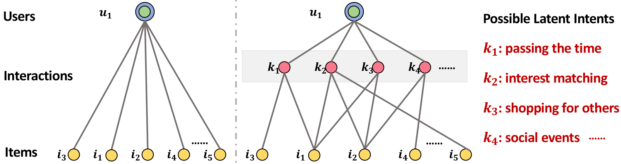
Figure 1. An illustration of diverse user-item relationships at the granularity of latent intents.

Learning informative representations of users and items is of crucial importance to improving CF. To this end, the potentials of deepening user-item relationships become more apparent. Early models like matrix factorization (MF) (Rendle et al., 2009) forgo user-item relationships in the embedding function by individually projecting each user/item ID into a vectorized representation (aka. embedding). Some follow-on studies (Koren, 2008; He et al., 2018; Liang et al., 2018; Kabbur et al., 2013) introduce personal history as the pre-existing feature of a user, and integrate embeddings of historical items to enrich her representation. More recent works (Wang et al., 2019b; van den Berg et al., 2017; He et al., 2020) further organize all historical interactions as a bipartite user-item graph to integrate the multi-hop neighbors into the representations and achieved the state-of-the-art performance. We attribute such remarkable improvements to the modeling of user-item relationships, evolving from using only a single ID, to personal history, and then holistic interaction graph.

Despite effectiveness, we argue that prior manner of modeling user-item relationships is insufficient to discover disentangled user intents. The key reason is that existing embedding functions fail to differentiate user intents on different items — they either treat a user-item interaction as an isolated data instance (Rendle et al., 2009; He et al., 2017) or uniformly organize it as an edge in the interaction graph (Wang et al., 2019b; van den Berg et al., 2017; He et al., 2020) (as shown in the left of Figure 1) to train the neural networks. An underlying fact is omitted that: a user generally has multiple intents to adopt certain items; moreover, different intents could motivate different user behaviors (Ma et al., 2019a, b; Ying et al., 2019; Chen et al., 2019). Taking the right of Figure 1 as an example, user $u$ watches movie $i_{1}$ to pass time, while cares less about whether $i_{1}$’s attributes (e.g., director) match with her interests; on the other hand, $u$’s interaction with $i_{2}$ may be mainly driven by her special interests on its director. Leaving this fact untouched, previous modeling of user-item relationships is coarse-grained, which has several limitations: 1) Without considering the actual user intents could easily lead to suboptimal representations; 2) As noisy behaviors (e.g., random clicks) commonly exist in a user’s interaction history, confounding her intents makes the representations less robust to noisy interactions; and 3) User intents will be obscure and highly entangled in representations, which results in poor interpretability.

Having realized the vital role of user-item relationships and the limitations of prior embedding functions, we focus on exploring the relationships at a more granular level of user intents, to disentangle these factors in the representations. Intuitively, there are multiple intents affecting a user’s behavior, such as to pass time, interest matching, or shopping for others like families. We need to learn a distribution over user intents for each user behavior, summarizing the confidence of each intent being the reason why a user adopts an item. Jointly analyzing such distributions of all historical interactions, we can obtain a set of intent-aware interaction graphs, which further distill the signals of user intents. However, this is not trivial due to the following challenges:

• How to explicitly present signals pertinent to each intent in a representation is unclear and remains unexplored;

• The quality of disentanglement is influenced by the independence among intents, which requires a tailored modeling.

In this work, we develop a new model, Disentangled Graph Collaborative Filtering (DGCF), to disentangle representations of users and items at the granularity of user intents. In particular, we first slice each user/item embedding into chunks, coupling each chunk with a latent intent. We then apply an graph disentangling module equipped with neighbor routing (Sabour et al., 2017; Ma et al., 2019a) and embedding propagation (Kipf and Welling, 2017; Hamilton et al., 2017; Wang et al., 2019b, a) mechanisms. More formally, neighbor routing exploits a node-neighbor affinity to refine the intent-aware graphs, highlighting the importance of influential relationships between users and items. In turn, embedding propagation on such graphs updates a node’s intent-aware embedding. By iteratively performing such disentangling operations, we establish a set of intent-aware graphs and chunked representations. Simultaneously, an independence modeling module is introduced to encourage independence of different intents. Specifically, a statistic measure, distance correlation (Székely et al., 2007; Székely et al., 2009), is employed on intent-aware representations. As the end of these steps, we obtain the disentangled representations, as well as explanatory graphs for intents. Empirically, DGCF is able to achieve better performance than the state-of-the-art methods such as NGCF (Wang et al., 2019b), MacridVAE (Ma et al., 2019b), and DisenGCN (Ma et al., 2019a) on three benchmark datasets.

We further make in-depth analyses on DGCF’s disentangled representations w.r.t. disentanglement and interpretability. To be more specific, we find that the discovered intents serve as vitamin to representations — that is, even in small quantities could achieve comparable performance, while the deficiency of any intent would hinder the results severely. Moreover, we use side information (i.e., user reviews) to help interpret what information are being captured in the intent-aware graphs, trying to understand the semantics of intents.

In a nutshell, this work makes the following main contributions:

• We emphasize the importance of diverse user-item relationships in collaborative filtering, and modeling of such relationships could lead to better representations and interpretability.

• We propose a new model DGCF, which considers user-item relationships at the finer granularity of user intents and generates disentangled representations.

• We conduct extensive experiments on three benchmark datasets, to demonstrate the advantages of our DGCF on the effectiveness of recommendation, disentanglement of latent user intents, and interpretability of representations.

2. Preliminary and Related Work

We first introduce the representation learning of CF, emphasizing the limitations of existing works w.r.t. the modeling of user-item relationships. In what follows, we present the task formulation of disentangling graph representations for CF.

2.1. Learning for Collaborative Filtering

Discovering user preference on items, based solely on user behavior data, lies in the core of CF modeling. Typically, the behavior data involves a set of users $\mathcal{U}=\{u\}$, items $\mathcal{I}=\{i\}$, and their interactions $\mathcal{O}^{+}=\{y_{ui}\}$, where $y_{ui}=1$ is an observed interaction indicating that user $u$ adopted item $i$ before, otherwise $0$. Hence, the prime task of CF is to predict how likely user $u$ would adopt item $i$, or more formally, the likelihood of their interaction $\hat{y}_{ui}$.

2.1.1. Learning Paradigm of CF

There exists a semantic gap between user and item IDs — no overlapping between such superficial features — hindering the interaction modeling. Towards closing this gap, extensive studies have been conducted to learn informative representations of users and items. Here we summarize the representation learning as follows:

(1) $$\mathbf{e}_{u}=f(u),\quad\mathbf{e}_{i}=f(i),$$

where $u$ and $i$ separately denote the user and item IDs; $\mathbf{e}_{u}\in\mathbb{R}^{d}$ and $\mathbf{e}_{i}\in\mathbb{R}^{d}$ are the vectorized representations (aka. embeddings) of user $u$ and item $i$, respectively; $f(\cdot)$ is the embedding function and $d$ is the embedding size. Such embeddings are expected to memorize underlying characteristics of items and users.

Thereafter, interaction modeling is performed to reconstruct the historical interactions. Inner product is a widely-used interaction function (Rendle et al., 2009; Wang et al., 2019b; Koren et al., 2009; Yang et al., 2018), which is employed on user and item representations to perform the prediction, as:

(2) $$\hat{y}_{ui}={\mathbf{e}}^{\top}_{u}\mathbf{e}_{i},$$

which casts the predictive task as the similarity estimation between $u$ and $i$ in the same latent space. Here we focus on the representation learning of CF, thereby using inner product as the predictive model and leaving the exploration of interaction modeling in future work.

2.1.2. Representation Learning of CF

Existing works leverage user-item relationships to enrich CF representations, evolving from single user-item pairs, personal history to the holistic interaction graph. Early, MF (Rendle et al., 2009; Koren et al., 2009; Salakhutdinov et al., 2007) projects each user/item ID into an embedding vector. Many recommenders, such as NCF (He et al., 2017), CMN (Ebesu et al., 2018), and LRML (Tay et al., 2018) resort to this paradigm. However, such paradigm treats every user-item pair as an isolated data instance, without considering their relationships in the embedding function. Towards that, later studies like SVD++ (Koren, 2008), FISM (Kabbur et al., 2013), NAIS (He et al., 2018), and ACF (Chen et al., 2017) view personal history of a user as her features, and integrate embeddings of historical items via the average (Koren, 2008; Kabbur et al., 2013) or attention network (He et al., 2018; Chen et al., 2017) as user embeddings, showing promise in representation learning. Another similar line applies autoencoders on interaction histories to estimate the generative process of user behaviors, such as Mult-VAE (Liang et al., 2018), AutoRec (Sedhain et al., 2015), and CDAE (Wu et al., 2016). One step further, the holistic interaction graph is used to smooth or enrich representations. Prior efforts like HOP-Rec (Yang et al., 2018) and GRMF (Rao et al., 2015) apply idea of unsupervised representation learning — that is, connected nodes have similar representations — to smooth user and item representations. More recently, inspired by the great success of graph neural networks (GNNs) (Kipf and Welling, 2017; Velickovic et al., 2018; Hamilton et al., 2017; Wu et al., 2019), some works, such as GC-MC (van den Berg et al., 2017), NGCF (Wang et al., 2019b), PinSage (Ying et al., 2018), and LightGCN (He et al., 2020), further reorganize personal histories in a graph, and distill useful information from multi-hop neighbors to refine the embeddings.

In the view of interaction graph, we can revisit such user-item relationships as the connectivity between user and item nodes. In particular, bipartite user-item graph is denoted as $\mathcal{G}=\{(u,i,y_{ui})\}$, where the edge between user $u$ and item $i$ nodes is the observed interaction $y_{ui}$. When exploring $\mathcal{G}$, connectivity is derived from a path starting from a user (or item) node, which carries rich semantic representing user-item relationships. Examining paths rooted at $u_{1}$, we have the first-order connectivity $u_{1}\rightarrow\{i_{1},i_{2}\}$ showing her interaction history, which intuitively profiles her interests; moreover, the second-order connectivity $u_{1}\rightarrow i_{1}\rightarrow u_{2}$ indicates behavioral similarity between $u_{1}$ and $u_{2}$, as both adopted $i_{1}$ before; furthermore, we exhibit collaborative signals via the third-order connectivity $u_{1}\rightarrow i_{1}\rightarrow u_{2}\rightarrow i_{3}$, which suggests that $u_{1}$ is likely to consume $i_{3}$ since her similar user $u_{2}$ has adopted $i_{3}$.

As such, user-item relationships can be explicitly represented as the connectivity: single ID (i.e., no connectivity) (Rendle et al., 2009), personal history (i.e., the first-order connectivity) (Koren, 2008), to holistic interaction graph (i.e., higher-order connectivity) (Wang et al., 2019b; Du et al., 2018; Yang et al., 2018).

2.1.3. Limitations

Despite of their success, we argue that such uniform modeling of user-item relationships is insufficient to reflect users’ latent intents. This limiting the interpretability and understanding of CF representations. To be more specific, present embedding functions largely employ a black-box neural network on the relationships (e.g., interaction graph $\mathcal{G}$), and output representations. They fail to differentiate user intents on different items by just presuming a uniform motivation behind behaviors. However, it violates the fact that a user generally has multiple intents when purchasing items. For example, user $u$ interacts with items $i_{1}$ and $i_{2}$ with intent to pass time and match personal taste, respectively. However, such latent intents are less explored, and could easily lead to suboptimal representation ability.

Without modeling such user intents, existing works hardly offer interpretable embeddings, so as to understand semantics or what information are encoded in particular dimensions. Specifically, the contributions of each interaction $(u,i)$ to all dimensions of $\mathbf{e}_{u}$ are indistinguishable. As a result, the latent intents behind each behavior are highly entangled in the embeddings, obscuring the mapping between intents and particular dimensions.

Study on disentangling representations for recommendation is less conducted until recent MacridVAE (Ma et al., 2019b). It employs $\beta$-VAE (Higgins et al., 2017) on interaction data and achieves disentangled representations of users. Owing to the limitations of $\beta$-VAE, only distributions over historical items (i.e., the first-order connectivity between users and items) are used to couple the discovered factors with user intents, while ignoring the complex user-item relationships (i.e., higher-order connectivity reflecting collaborative signals). We hence argue that the user-item relationships might be not fully explored in MacridVAE.

2.2. Task Formulation

We formulate our task that consists of two subtasks — 1) exploring user-item relationships at a granular level of user intents and 2) generating disentangled CF representations.

2.2.1. Exploring User-Item Relationships.

Intuitively, one user behavior is influenced by multiple intents, such as passing time, matching particular interests, and shopping for others like family. Taking movie recommendation as an example, user $u$ passed time with movie $i_{1}$, hence might care less about whether $i_{1}$’s director matches her interests well; whereas, $u$ watched $i_{2}$ since its director is an important factor of $u$’s interest. Clearly, different intents have varying contributions to motivate user behaviors.

To model such finer-grained relationships between users and items, we aim to learn a distribution $A(u,i)$ over user intents for each behavior, as follows:

(3) $$\mathbf{A}(u,i)=\Big{(}A_{1}(u,i),\cdots,A_{K}(u,i)\Big{)},$$

where $A_{k}(u,i)$ reflects the confidence of the $k$-th intent being the reason why user $u$ adopts item $i$; $K$ is the hyperparameter controlling the number of latent user intents. Jointly examining the scores relevant to particular intent $k$, we can construct an intent-aware graph $\mathcal{G}_{k}$, which is defined as $\mathcal{G}_{k}=\{(u,i,A_{k}(u,i))\}$, where each historical interaction $(u,i)$ represents one edge and is assigned with $A_{k}(u,i)$. Moreover, a weighted adjacency matrix $\mathbf{A}_{k}$ is built for $\mathcal{G}_{k}$. As such, we establish a set of intent-aware graphs $\mathcal{G}=\{\mathcal{G}_{1},\cdots,\mathcal{G}_{K}\}$ to present diverse user-item relationships, instead of a uniform one adopted in prior works (Wang et al., 2019b; He et al., 2020; van den Berg et al., 2017).

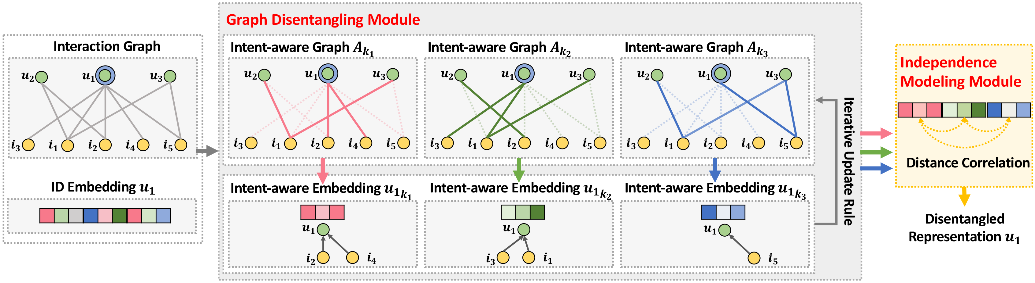
Figure 2. Illustration of the proposed disentangled graph collaborative filtering framework. Best viewed in color.

2.2.2. Generating Disentangled Representations.

We further target at exploiting the discovered intents to generate disentangled representations for users and items — that is, extract information that are pertinent to individual intents as independent parts of representations. More formally, we aim to devise an embedding function $f(\cdot)$, so as to output a disentangled representation $\mathbf{e}_{u}$ for user $u$, which is composed of $K$ independent components:

(4) $$\mathbf{e}_{u}=(\mathbf{e}_{1u},\mathbf{e}_{2u},\cdots,\mathbf{e}_{Ku}),$$

where $\mathbf{e}_{ku}$ is the $k$-th latent intent influence for user $u$; for simplicity, we make these component the same dimension, $\mathbf{e}_{ku}\in\mathbb{R}^{\frac{d}{K}}$. It is worth highlighting that $e_{ku}$ should be independent of $\mathbf{e}_{k^{\prime}u}$ for $k^{\prime}\neq k$, so as to reduce semantic redundancy and encourage that signals are maximally compressed about individual intents. Towards that, each chunked representation $\mathbf{e}_{ku}$ is built upon the intent-aware graph $\mathcal{G}_{k}$ and synthesizes the relevant connectivities. Analogously, we can establish the representation $\mathbf{e}_{i}$ for item $i$.

3. Methodology

We now present disentangled graph collaborative filtering, termed DGCF, which is illustrated in Figure 2. It is composed of two key components to achieve disentanglement: 1) graph disentangling module, which first slices each user/item embedding into chunks, coupling each chunk with an intent, and then incorporates a new neighbor routing mechanism into graph neural network, so as to disentangle interaction graphs and refine intent-aware representations; and 2) independence modeling module, which hires distance correlation as a regularizer to encourage independence of intents. DGCF ultimately yields disentangled representations with intent-aware explanatory graphs.

3.1. Graph Disentangling Module

Studies on GNNs (Kipf and Welling, 2017; Velickovic et al., 2018; Hamilton et al., 2017) have shown that applying embedding-propagation mechanism on graph structure can extract useful information from multi-hop neighbors and enrich representation of the ego node. To be more specific, a node aggregates information from its neighbors and updates its representations. Clearly, the connectivities among nodes provide an explicit channel to guide the information flow. We hence develop a GNN model, termed graph disentangling layer, which incorporates a new neighbor routing mechanism into the embedding propagation, so as to update weights of these graphs. This allows us to differentiate varying importance scores of each user-item connection to refine the interaction graphs, and in turn propagate signals to the intent-aware chunks.

3.1.1. Intent-Aware Embedding Initialization

Distinct from mainstream CF models (Rendle et al., 2009; Wang et al., 2019b; Koren, 2008; He et al., 2017) that parameterize user/item ID as a holistic representation only, we additionally separate the ID embeddings into $K$ chunks, associating each chunk with a latent intent. More formally, such user embedding is initialized as:

(5) $$\mathbf{u}=(\mathbf{u}_{1},\mathbf{u}_{2},\cdots,\mathbf{u}_{K}),$$

where $\mathbf{u}\in\mathbb{R}^{d}$ is ID embedding to capture intrinsic characteristics of $u$; $\mathbf{u}_{k}\in\mathbb{R}^{\frac{d}{K}}$ is $u$’s chunked representation of the $k$-th intent. Analogously, $\mathbf{i}=(\mathbf{i}_{1},\mathbf{i}_{2},\cdots,\mathbf{i}_{K})$ is established for item $i$. Hereafter, we separately adopt random initialization to initialize each chunk representation, to ensure the difference among intents in the beginning of training. It is worth highlighting that, we set the same embedding size (say $d=64$) with the mainstream CF baselines, instead of doubling model parameters (cf. Section 3.4.1).

3.1.2. Intent-Aware Graph Initialization

We argue that prior works are insufficient to profile rich user intents behind behaviors, since they only utilize one user-item interaction graph (Wang et al., 2019b) or homogeneous rating graphs (van den Berg et al., 2017) to exhibit user-item relationships. Hence, we define a set of score matrices $\{\mathbf{S}_{k}|\forall k\in\{1,\cdots,K\}\}$ for $K$ latent intents. Focusing on an intent-aware matrix $\mathbf{S}_{k}$, each entry $S_{k}(u,i)$ denotes the interaction between user $u$ and item $i$. Furthermore, for each interaction, we can construct a score vector $\mathbf{S}(u,i)=(S_{1}(u,i),\cdots,S_{K}(u,i))\in\mathbb{R}^{K}$ over $K$ latent intents. We uniformly initialize each score vectors as follows:

(6) $$\mathbf{S}(u,i)=(1,\cdots,1),$$

which presumes the equal contributions of intents at the start of modeling. Hence, such score matrix $\mathbf{S}_{k}$ can be seen as the adjacency matrix of intent-aware graph.

3.1.3. Graph Disentangling Layer

Each intent $k$ now includes a set of chunked representations, $\{\mathbf{u}_{k},\mathbf{i}_{k}|u\in\mathcal{U},i\in\mathcal{I}\}$, which specialize its feature space, as well as a specific interaction graph represented by $\mathbf{S}_{k}$. Within individual intent channels, we aim to distill useful information from high-order connectivity between users and items, going beyond ID embeddings. Towards this end, we devise a new graph disentangling layer, which is equipped with the neighbor routing and embedding propagation mechanisms, with the target of differentiating adaptive roles of each user-item connection when propagating information along it. We define such layer $g(\cdot)$ as follows:

(7) $$\mathbf{e}^{(1)}_{ku}=g(\mathbf{u}_{k},\{\mathbf{i}_{k}|i\in\mathcal{N}_{u}\}),$$

where $\mathbf{e}^{(1)}_{ku}$ is to collect information that are pertinent to intent $k$ from $u$’s neighbors; $\mathcal{N}_{u}$ is the first-hop neighbors of $u$ (i.e., the historical items adopted by $u$); and the super-index $(1)$ denotes the first-order neighbors.

Iterative Update Rule. Thereafter, as Figure 3 shows, the neighbor routing mechanism is adopted: first, we employ the embedding propagation mechanism to update the intent-aware embeddings, based on the intent-aware graphs; then, we in turn utilize the updated embeddings to refine the graphs and output the distributions over intents. In particular, we set $T$ iterations to achieve such iterative update. In each iteration $t$, $\mathbf{S}^{t}_{k}$ and $\mathbf{u}^{t}_{k}$ separately memorize the updated values of adjacency matrix and embeddings, where $t\in\{1,2,\cdots,T\}$ and $T$ is the terminal iteration. It starts by initializing $\mathbf{S}^{0}_{k}=\mathbf{S}_{k}$ and $\mathbf{u}^{0}_{k}=\mathbf{u}_{k}$ via Equations (6) and (5).

Cross-Intent Embedding Propagation. At iteration $t$, for the target interaction $(u,i)$, we have the score vector, say $\{\mathbf{S}_{k}(u,i)|\forall k\in\{1,\cdots,K\}\}$. To obtain its distribution over all intents, we then normalize these coefficients via the softmax function:

(8) $$\tilde{S}^{t}_{k}(u,i)=\frac{\exp{S^{t}_{k}(u,i)}}{\sum_{k^{\prime}=1}^{K}\exp{S^{t}_{k^{\prime}}(u,i)}},$$

which is capable of illustrating which intents should get more attention to explain each user behavior $(u,i)$. As a result, we can get the normalized adjacency matrix $\tilde{\mathbf{S}}^{t}_{k}$ for each intent $k$. We then perform embedding propagation (Kipf and Welling, 2017; Velickovic et al., 2018; Hamilton et al., 2017) over individual graphs, such that the information, which are influential to the user intent $k$, are encoded into the representations. More formally, the weighted sum aggregator is defined as:

(9) $$\mathbf{u}^{t}_{k}=\sum_{i\in\mathcal{N}_{u}}\mathcal{L}^{t}_{k}(u,i)\cdot\mathbf{i}^{0}_{k},$$

where $\mathbf{u}^{t}_{k}$ is $u$’s temporary representation to memorize signals refined from her neighbors $\mathcal{N}_{u}=\{i|(u,i)\in\mathcal{G}\}$, after $t$ iterations; $\mathbf{i}^{0}_{k}$ is the input representation for historical item $i$; and and $\mathcal{L}^{t}_{k}(u,i)$ is the Laplacian matrix of $\tilde{\mathbf{S}}^{t}_{k}$, formulated as:

(10) $$\mathcal{L}^{t}_{k}(u,i)=\frac{\tilde{S}^{t}_{k}(u,i)}{\sqrt{D^{t}_{k}(u)\cdot D^{t}_{k}(i)}},$$

where $D^{t}_{k}(u)=\sum_{i^{\prime}\in\mathcal{N}_{u}}\tilde{S}^{t}_{k}(u,i^{\prime})$ and $D^{t}_{k}(i)=\sum_{u^{\prime}\in\mathcal{N}_{i}}\tilde{S}^{t}_{k}(u^{\prime},i)$ are the degrees of user $u$ and item $i$, respectively; $N_{u}$ and $N_{i}$ are the one-hop neighbors of $u$ and $i$, respectively. Obviously, when iteration $t=1$, $D^{1}_{k}(u)$ and $D^{1}_{k}(i)$ separately degrade as $|\mathcal{N}_{u}|$ and $|\mathcal{N}_{i}|$, which is the fixed decay term widely adopted in prior studies (Kipf and Welling, 2017; Wu et al., 2019). Such normalization can handle the varying neighbor numbers of nodes, making the training process more stable.

It is worth emphasizing that, we aggregate the initial chunked representations $\{\mathbf{i}^{0}_{k}\}$ as the distilled information for user $u$. This contains the signal from the first-order connectivities only, while excluding that from user $u$ herself and her higher-hop neighbors. Moreover, inspired by recent SGC (Wu et al., 2019) and LightGCN (He et al., 2020), we argue that nonlinear transformation adopted by prior works (Wang et al., 2019b; van den Berg et al., 2017) is burdensome for CF and its black-box nature hinders the disentanglement process, thereby omitting the transformation and using ID embeddings only.

Intent-Aware Graph Update. We iteratively adjust the edge strengths based on neighbors of a user (or an item) node. Examining the subgraph structure rooted at user node $u$ with Equation (9), $\mathbf{u}^{t}_{k}$ can be seen as the centroid within the local pool $\mathcal{N}_{u}=\{(u,i)\}$, which contains items $u$ has interacted with before. Intuitively, historical items driven by the same intent tend to have similar chunked representations, further encouraging their relationships to be stronger. We hence iteratively update $S^{t}_{k}(u,i)$ — more precisely, adjusting the strength between the centroid $u$ and its neighbor $i$, as follows:

(11) $$S^{t+1}_{k}(u,i)=S^{t}_{k}(u,i)+{\mathbf{u}^{t}_{k}}^{\top}\text{tanh}(\mathbf{i}^{0}_{i}),$$

where ${\mathbf{u}^{t}_{k}}^{\top}\text{tanh}(\mathbf{i}^{0}_{k})$ considers the affinity between $\mathbf{u}^{t}_{k}$ and $\mathbf{i}^{0}_{k}$; and tanh (Vaswani et al., 2017) is a nonlinear activation function to increase the representation ability of model.

After $T$ iterations, we ultimately obtain the output of one graph disentangling layer, which consists of disentangled representation i.e., $\mathbf{e}^{(1)}_{ku}=\mathbf{u}^{T}_{k}$, as well as its intent-aware graph i.e., $\mathbf{A}^{(1)}_{k}=\tilde{\mathbf{S}}^{T}_{k}$, $\forall k\in\{1,\cdots,K\}$. When performing such propagation forward, our model aggregates information pertinent to each intent and generates an attention flow, which can be viewed as explanations behind the disentanglement.

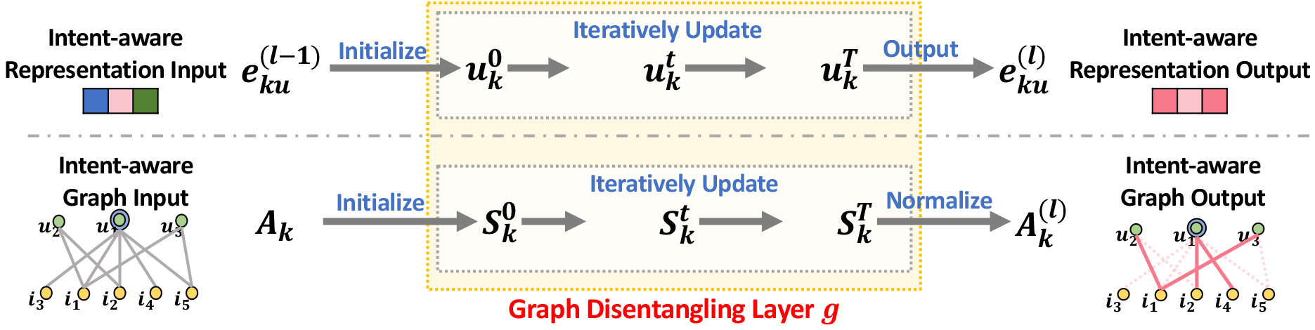
Figure 3. Illustration of iterative update rule.

3.1.4. Layer Combination

Having used the first-hop neighbors, we further stack more graph disentangling layers to gather the influential signals from higher-order neighbors. In particular, such connectivities carry rich semantics. For instance, the second-order connectivity like $u_{1}\rightarrow i_{2}\rightarrow u_{3}$ suggests the intent similarity between $u_{1}$ and $u_{3}$ when consuming $i_{2}$; meanwhile, the longer path $u_{1}\rightarrow i_{2}\rightarrow u_{2}\rightarrow i_{4}$ deepens their intents via the collaborative signal. To capture user intents from such higher-order connectivity, we recursively formulate the representation after $l$ layers as:

(12) $$\mathbf{e}^{(l)}_{ku}=g\Big{(}\mathbf{e}^{(l-1)}_{ku},\{\mathbf{e}^{(l-1)}_{ki}|i\in\mathcal{N}_{u}\}\Big{)},$$

where $\mathbf{e}^{(l-1)}_{ku}$ and $\mathbf{e}^{(l-1)}_{ki}$ are the representations of user $u$ and item $i$ conditioned on the $k$-th factor, memorizing the information being propagated from their $(l-1)$-hop neighbors. Moreover, each disentangled representation is also associated with its explanatory graphs to explicitly present the intents, i.e., the weighted adjacency matrix $\mathbf{A}^{(l)}_{k}$. Such explanatory graphs are able to show reasonable evidences of what information construct the disentangled representations.

After $L$ layers, we sum the intent-aware representations at different layers up as the final representations, as follows:

(13) $$\mathbf{e}_{ku}=\mathbf{e}^{(0)}_{ku}+\cdots+\mathbf{e}^{(L)}_{ku},\quad\quad\mathbf{e}_{ki}=\mathbf{e}^{(0)}_{ki}+\cdots+\mathbf{e}^{(L)}_{ki}.$$

By doing so, we not only disentangle the CF representations, but also have the explanations for each part of representations. It is worthwhile to emphasize that the trainable parameters are only the embeddings at the $0$-th layer, i.e., $\mathbf{u}$ and $\mathbf{i}$ for all users and items (cf. Equation (5)).

3.2. Independence Modeling Module

As suggested in (Sabour et al., 2017; Ma et al., 2019a), dynamic routing mechanism encourages the chunked representations conditioned on different intents to be different from each others. However, the difference constraint enforced by dynamic routing is insufficient: there might be redundancy among factor-aware representations. For example, if one intent-aware representation $\mathbf{u}_{k}$ can be inferred by the others $\{\mathbf{u}_{k^{\prime}}|k^{\prime}\neq k\}$, the factor $k$ is highly likely to be redundant and could be confounding.

We hence introduce another module, which can hire statistical measures like mutual information (Belghazi et al., 2018) and distance correlation (Székely et al., 2007; Székely et al., 2009) as a regularizer, with the target of encouraging the factor-aware representations to be independent. We here apply distance correlation, leaving the exploration of mutual information in future work. In particular, distance correlation is able to characterize independence of any two paired vectors, from their both linear and nonlinear relationships; its coefficient is zero if and only if these vectors are independent (Székely et al., 2007). We formulate this as:

(14) $$loss_{\text{ind}}=\sum^{K}_{k=1}\sum^{K}_{k^{\prime}=k+1}dCor(\mathbf{E}_{k},\mathbf{E}_{k^{\prime}}),$$

where $\mathbf{E}_{k}=[\mathbf{e}_{u_{1}k},\cdots,\mathbf{e}_{u_{N}k},\mathbf{e}_{i_{1}k},\cdots,\mathbf{e}_{i_{M}k}]\in\mathbb{R}^{(M+N)\times\frac{d}{K}}$ is the embedding look-up table with $N=|\mathcal{U}|$ and $M=|\mathcal{I}|$, which is built upon the intent-aware representations of all users and items; and, $dCor(\cdot)$ is the function of distance correlation defined as:

(15) $$dCor(\mathbf{E}_{k},\mathbf{E}_{k^{\prime}})=\frac{dCov(\mathbf{E}_{k},\mathbf{E}_{k^{\prime}})}{\sqrt{dVar(\mathbf{E}_{k})\cdot dVar(\mathbf{E}_{k^{\prime}})}}$$

where $dCov(\cdot)$ represents the distance covariance between two matrices; $dVar(\cdot)$ is the distance variance of each matrix. For a more detailed calculation, refer to prior works (Székely et al., 2007).

3.3. Model Optimization

Having obtained the final representations for user $u$ and item $i$, we use inner product (cf. Equation (2)) as the predictive function to estimate the likelihood of their interaction, $\hat{y}_{ui}$. Thereafter, we use the pairwise BPR loss (Rendle et al., 2009) to optimize the model parameters $\Theta=\{\mathbf{u},\mathbf{i}|u\in\mathcal{U},i\in\mathcal{I}\}$. Specifically, it encourages the prediction of a user’s historical items to be higher than that of unobserved items:

(16) $$loss_{\text{BPR}}=\sum_{(u,i,j)\in\mathcal{O}}-\ln{\sigma(\hat{y}_{ui}-\hat{y}_{uj})}+\lambda\left\lVert\Theta\right\rVert^{2}_{2},$$

where $\mathcal{O}=\{(u,i,j)|(u,i)\in\mathcal{O}^{+},(u,j)\in\mathcal{O}^{-}\}$ denotes the training dataset involving the observed interactions $\mathcal{O}^{+}$ and unobserved counterparts $\mathcal{O}^{-}$; $\sigma(\cdot)$ is the sigmoid function; $\lambda$ is the coefficient controlling $L_{2}$ regularization. During the training, we alternatively optimize the independence loss (cf. Equation (14)) and BPR loss (cf. Equation (16)).

3.4. Model Analysis

In this subsection, we conduct model analysis, including the complexity analysis and DGCF’s relations with existing models.

3.4.1. Model Size

While we slice the embeddings into $K$ chunks, the total embedding size remains the same as that set in MF and NGCF (i.e., $d=64$). That is, our DGCF involves no additional model parameters to learn, whole trainable parameters are $\{\mathbf{u},\mathbf{i}|u\in\mathcal{U},i\in\mathcal{I}\}$. The model size of DGCF is identical to MF and lighter than NGCF that introduces additional transformation matrices.

3.4.2. Relation with LightGCN

LightGCN (He et al., 2020) can be viewed as a special case of DGCF with only-one intent representation and no independence modeling. As the same datasets and experimental settings are used in these two models, we can directly compare DGCF with the empirical results reported in the LightGCN paper. In terms of the recommendation accuracy, DGCF and LightGCN are in the same level. However, benefiting from the disentangled representations, our DGCF has better interpretability since it can disentangle the latent intents in user representations (evidence from Table 4), and further exhibit the semantics of user intents (evidence from Section 4.4.2), while LightGCN fails to offer explainable representations.

3.4.3. Relation with Capsule Network

From the perspective of capsule networks (Sabour et al., 2017; Hinton et al., 2011), we can view the chunked representations as the capsules and the iterative update rule as the dynamic routing. However, distinct from typical capsule networks that adopt the routing across different layers, DGCF further incorporate the routing with the embedding propagation of GNNs, such that not only can the information be passed across layers, but also be propagated within the neighbors within the same layer. As a result, our DGCF is able to distill useful information, that are relevant to intents, from multi-hop neighbors.

3.4.4. Relation with Multi-head Attetion Network

Although the intent-aware graphs can been seen as channels used in multi-head attention mechanism (Vaswani et al., 2017; Velickovic et al., 2018), they have different utilities. Specifically, multi-head attention is mainly used to stabilize the learning of attention network (Velickovic et al., 2018) and encourage the consistence among different channels; whereas, DGCF aims to collect different signals and leverage the independence module (cf. Section 3.2) to enforce independence of intent-aware graphs. Moreover, there is no information interchange between attention networks, while DGCF allows the intent-aware graphs to influence each other.

3.4.5. Relation with DisenGCN

DisenGCN (Ma et al., 2019a) is proposed to disentangle latent factors for graph representations, where the neighbor routing is also coupled with GNN models. Our DGCF distinguishes from DisenGCN from several aspects: 1) DisenGCN fails to model the independence between factors, easily leading to redundant representations, while DGCF applies the distance correlation to achieve independence; 2) the embedding propagation in DisenGCN mixes the information from the ego node self and neighbors together; whereas, DGCF can purely distill information from neighbors; and 3) DGCF’s neighbor routing (cf. Section 3.1.3) is more effective than that of DisenGCN (cf. Section 4.2).

4. Experiments

Table 1. Statistics of the datasets.

Dataset	#Users	#Items	#Interactions	Density
Gowalla	$29,858$	$40,981$	$1,027,370$	$0.00084$
Yelp2018∗	$31,668$	$38,048$	$1,561,406$	$0.00130$
Amazon-Book	$52,643$	$91,599$	$2,984,108$	$0.00062$

To answer the following research questions, we conduct extensive experiments on three public datasets:

• RQ1: Compared with present models, how does DGCF perform?

• RQ2: How different components (e.g., layer number, intent number, independence modeling) affect the results of DGCF?

• RQ3: Can DGCF provide in-depth analyses of disentangled representations w.r.t. disentanglement of latent user intents and interpretability of representations?

4.1. Experimental Settings

4.1.1. Dataset Description

We use three publicly available datasets: Gowalla, Yelp2018^∗, and Amazon-Book, released by NGCF (Wang et al., 2019b). Note that we revise Yelp2018 dataset, as well as the updated results of baselines, instead of the original reported in the NGCF paper (Wang et al., 2019b). We denote the revised as Yelp2018^∗. The statistics of datasets are summarized in Table 1. We closely follow NGCF and use the same data split as NGCF. In the training phase, each observed user-item interaction is treated as a positive instance, while we use negative sampling to randomly sample an unobserved item and pair it with the user as a negative instance.

4.1.2. Baselines

We compare DGCF with the state-of-the-art methods, covering the CF-based (MF), GNN-based (GC-MC and NGCF), disentangled GNN-based (DisenGCN), and disentangled VAE-based (MacridVAE):

• MF (Rendle et al., 2009): Such model treats user-item interactions as isolated data instances, and only uses ID embeddings as representations of users and items.

• GC-MC (van den Berg et al., 2017): The method organizes historical user behaviors as a holistic interaction graph, and employs one GCN (Kipf and Welling, 2017) encoder to generate representations. Note that only one-hop neighbors are involved.

• NGCF (Wang et al., 2019b): This adopts three GNN layers on the user-item interaction graph, aiming to refine user and item representations via at most three-hop neighbors’ information.

• DisenGCN (Ma et al., 2019a): This is a state-of-the-art disentangled GNN model, which exploits the neighbor routing and embedding propagation to disentangle latent factors behind graph edges.

• MacridVAE (Ma et al., 2019b): Such model is tailored to disentangle user intents behind user behaviors. In particular, it adopts $\beta$-VAE to estimate the generative process of a user’s personal history, assuming that there are several latent factors affecting user behaviors, to achieved disentangled user representations.

4.1.3. Evaluation Metrics.

To evaluate top-$N$ recommendation, we use the same protocols as NGCF (Wang et al., 2019b): recall@$N$ and ndcg@$N$, where $N$ is set as $20$ by default. In the inference phase, we view historical items of a user in the test set as the positive, and evaluate how well these items are ranked higher than all unobserved ones. The average results w.r.t. the metrics over all users are reported.

4.1.4. Parameter Settings.

We implement the DGCF model in Tensorflow. For a fair comparison, we tune the parameter settings of each model. In particular, we directly copy the best performance of MF, GC-MC, and NGCF reported in the original paper (Wang et al., 2019b). As for DisenGCN and DGCF, we fix the embedding size $d$ as $64$ (which is identical to MF, GC-MC, and NGCF), use Adam (Kingma and Ba, 2015) as the optimizer, initialize model parameters with Xarvier (Glorot and Bengio, 2010), and fix the iteration number $T$ as $2$. Moreover, a grid search is conducted to confirm the optimal settings — that is, the learning rate is searched in $\{0.001,0.005,0.0005,0.0001\}$, and the coefficients $\lambda$ of $L_{2}$ regularization term is tuned in $\{10^{-3},10^{-4},10^{-5}\}$. For MacridVAE (Ma et al., 2019b), we search the number of latent factors being disentangled in $\{2,4,8,16\}$, and tune the factor size in $\{50,55,60,65,70\}$.

Without specification, unique hyperparameters of DGCF are set as: $L=1$ and $K=4$. We study the number of graph disentangling layer $L$ in $\{0,1,2,3\}$ and the number of latent intents $K$ in $\{2,4,8,16\}$, and report their influences in Sections 4.3.1 and 4.3.2, respectively.

Table 2. Overall Performance Comparison.

	Gowalla		Yelp2018∗		Amazon-Book
	recall	ndcg	recall	ndcg	recall	ndcg
MF	0.1291	0.1109	0.0433	0.0354	0.0250	0.0196
GC-MC	0.1395	0.1204	0.0462	0.0379	0.0288	0.0224
NGCF	0.1569	0.1327	0.0579	0.0477	0.0337	0.0266
DisenGCN	0.1356	0.1174	0.0558	0.0454	0.0329	0.0254
MacridVAE	0.1618	0.1202	0.0612	0.0495	0.0383	0.0295
DGCF-1	$\mathbf{0.1794}^{*}$	$\mathbf{0.1521}^{*}$	$\mathbf{0.0640}^{*}$	$\mathbf{0.0522}^{*}$	$\mathbf{0.0399}^{*}$	$\mathbf{0.0308}^{*}$
%improv.	10.88%	14.62%	4.58%	5.45%	4.17%	4.41%
$p$-value	6.63e-8	3.10e-7	1.75e-8	4.45e-9	8.26e-5	7.15e-5

4.2. Performance Comparison (RQ1)

We report the empirical results of all methods in Table 2. The improvements and statistical significance test are performed between DGCF-1 with the strongest baselines (highlighted with underline). Analyzing such performance comparison, we have the following observations:

• Our proposed DGCF achieves significant improvements over all baselines across three datasets. In particular, its relative improvements over the strongest baselines w.r.t. recall@$20$ are $10.88\%$, $4.58\%$, and $4.17\%$ in Gowalla, Yelp2018^∗, and Amazon-Book, respectively. This demonstrates the high effectiveness of DGCF. We attribute such improvements to the following aspects — 1) by exploiting diverse user-item relationships, DGCF is able to better characterize user preferences, than prior GNN-based models that treat the relationships as uniform edges; 2) the disentangling module models the representations at a more granular level of user intents, endowing the recommender better expressiveness; and 3) embedding propagation mechanism can more effectively distill helpful information from one-hop neighbors, than one-layer GC-MC and three-layer NGCF.

• Jointly analyzing the results across three datasets, we find that the improvements on Amazon-Book is much less than that on the others. This might suggest that, purchasing books is a simper scenario than visiting location-based business. Hence, the user intents on purchasing books are less diverse.

• MF performs poor on three datasets. This indicates that, modeling user-item interactions as isolated data instance could ignore underlying relationships among users and items, and easily lead to unsatisfactory representations.

• Compared with MF, GC-MC and NGCF consistently achieve better performance on three datasets, verifying the importance of user-item relationships. They take the one-hop neighbors (i.e., reflecting behavioral similarity of users) and third-hop neighbors (i.e., carrying collaborative signals) into representations.

• DisenGCN substantially outperforms GC-MC in most cases. It is reasonable since user intents are explicitly modeled as factors being disentangled in DisenGCN, which offer better guide to distill information from one-hop neighbors. However, its results are worse than that of DGCF. Possible reasons are that 1) its routing mechanism only uses node affinity to adjust the graph structure, without any priors to guide; and 2) many operations (e.g., nonlinear transformation) are heavy to CF (Wu et al., 2019). This suggests its suboptimal disentanglement.

• MacridVAE serves as the strongest baseline in most cases. This justifies the effectiveness of estimating personal history via a generative process, and highlights the importance of the disentangled representations.

4.3. Study of DGCF (RQ2)

Ablation studies on DGCF are also conducted to investigate the rationality and effectiveness of some designs — to be more specific, how the number of graph disentangling layers, the number of latent user intents, and independence modeling influence the model.

Table 3. Impact of Layer Number ($L$).

	Gowalla		Yelp2018∗		Amazon-Book
	recall	ndcg	recall	ndcg	recall	ndcg
DGCF-1	0.1794	0.1521	0.0640	0.0522	0.0399	0.0308
DGCF-2	0.1834	0.1560	0.0653	0.0532	0.0422	$\mathbf{0.0324}^{*}$
DGCF-3	$\mathbf{0.1842}^{*}$	$\mathbf{0.1561}^{*}$	$\mathbf{0.0654}^{*}$	$\mathbf{0.0534}^{*}$	$\mathbf{0.0422}^{*}$	0.0322

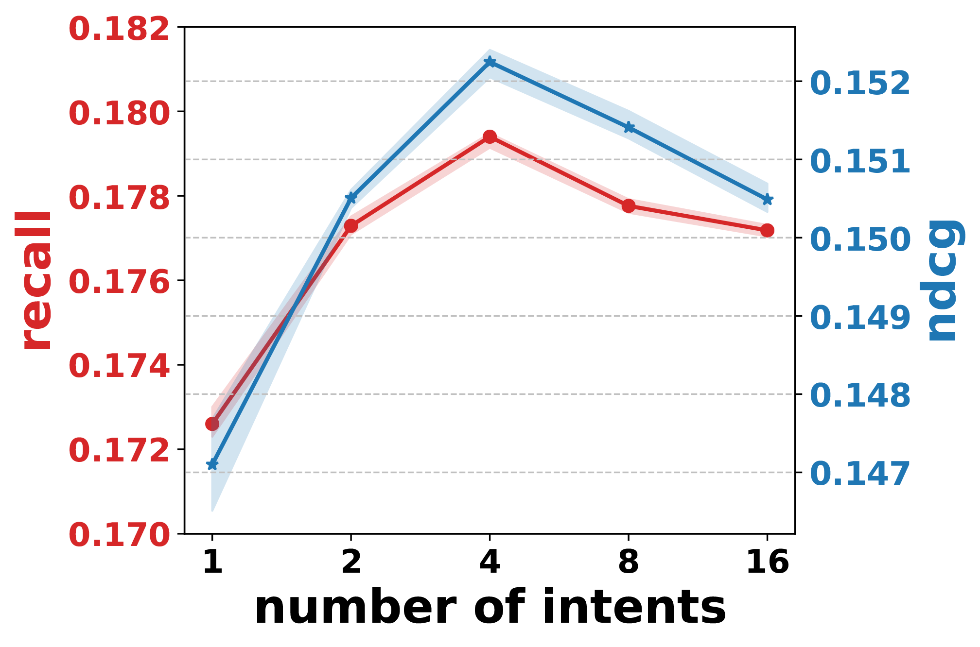
(a) Intent Impact in Gowalla

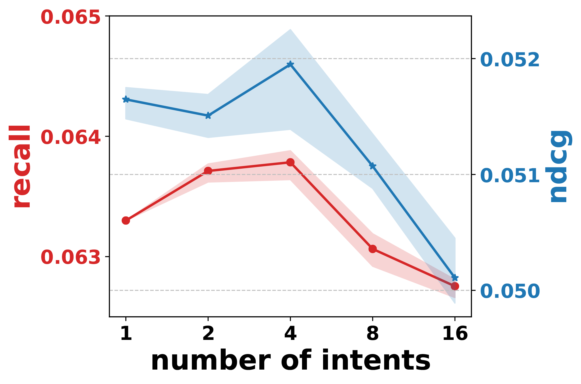
(b) Intent Impact in Yelp208^∗

Figure 4. Impact of Intent Number ($K$). Best Viewed in Color.

4.3.1. Impact of Model Depth.

The graph disentangling layer is at the core of DGCF, which not only disentangles user intents, but also collects information pertinent to individual intents into intent-aware representations. Furthermore, stacking more layers is able to distill the information from multi-hop neighbors. Here we investigate how the number of such layers, $L$, affects the performance. Towards that, we search $L$ in the range of $\{1,2,3\}$ and summarize the empirical results in Table 3. Here we use DGCF-1 to denote the recommender with one disentangling layer, and similar notations for others. We have several findings:

• Clearly, increasing the model depth is capable of endowing the recommender with better representation ability. In particular, DGCF-2 outperforms DGCF-1 by a large margin. This makes sense since DGCF-1 just gathers the signals from one-hop neighbors, while DGCF-2 considers multi-hop neighbors.

• While continuing stacking more layer beyond DGCF-2 gradually improves the performance of DGCF-3, the improvements are not that obvious. This suggests that the second-order connectivity might be sufficient to distill intent-relevant information. Such observation is consistent to NGCF (Wang et al., 2019b).

• We compare the results across Tables 2 and 3 and find that DGCF with varying depths is consistently superior to other baselines. This again verifies the effectiveness of embedding propagation with neighbor routing.

4.3.2. Impact of Intent Number.

To study the influence of intent number, we vary $K$ in range of $\{1,2,4,8,16\}$ and demonstrate the performance comparison on Gowalla and Yelp^∗ datasets in Figure 4. There are several observations:

• Increasing the intent number from $1$ to $4$ significantly enhances the performance. In particular, DGCF performs the worst when $K=1$, indicating that only uniform relationship is not sufficient to profile behavioral patterns of users. This again justifies the rationality of disentangling user intents.

• Interestingly, the recommendation performance drops when then intent number reaches $8$ and $16$. This suggests that, although benefiting from the proper intent chunks, the disentanglement suffers from too fine-grained intents. One possible reason is that the chunked representations only with the embedding size of $4$ (e.g., $\frac{d}{K}=4$ when $K=16$) have limited expressiveness, hardly describing a complete pattern behind user behaviors.

• Separately analyzing the performance in Gowalla and Yelp208^∗, we find that the influences of intent number are varying. We attribute this to the differences between scenarios. To be more specific, Gowalla is a location-based social networking service which provides more information, such as social marketing, as the intents than Yelp2018^∗. This indicates that user behaviors are driven by different intents for difference scenarios.

Table 4. Distance correlation of different methods (the lower the better).

	Gowalla	Yelp∗	Amazon-Book
MF	0.2332	0.2701	0.2364
NGCF	0.2151	0.2560	0.1170
DGCF-1	0.1389	0.1713	0.1039
DGCF-2	$\mathbf{0.0920}^{*}$	$\mathbf{0.1217}^{*}$	$\mathbf{0.0751}^{*}$

Table 5. Impact of Independence w.r.t. recall in Yelp2018^∗.

	DGCF-1	DGCF-2	DGCF-3
w/o ind	0.0637	0.0649	0.0650
w/ ind	0.0640	0.0653	0.0654

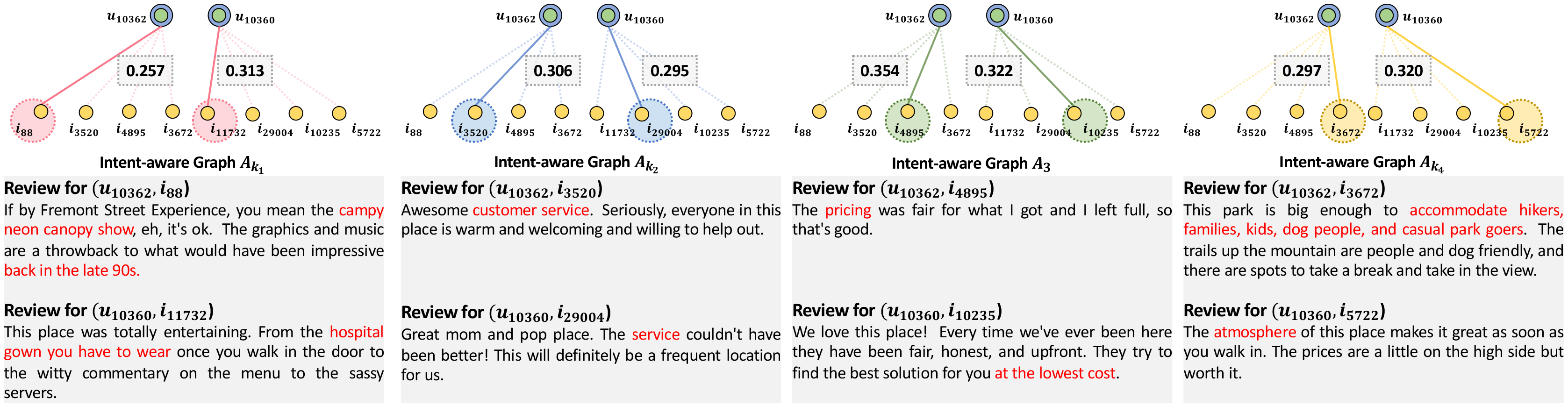
Figure 5. Illustration of the proposed disentangled graph collaborative filtering framework. Best viewed in color.

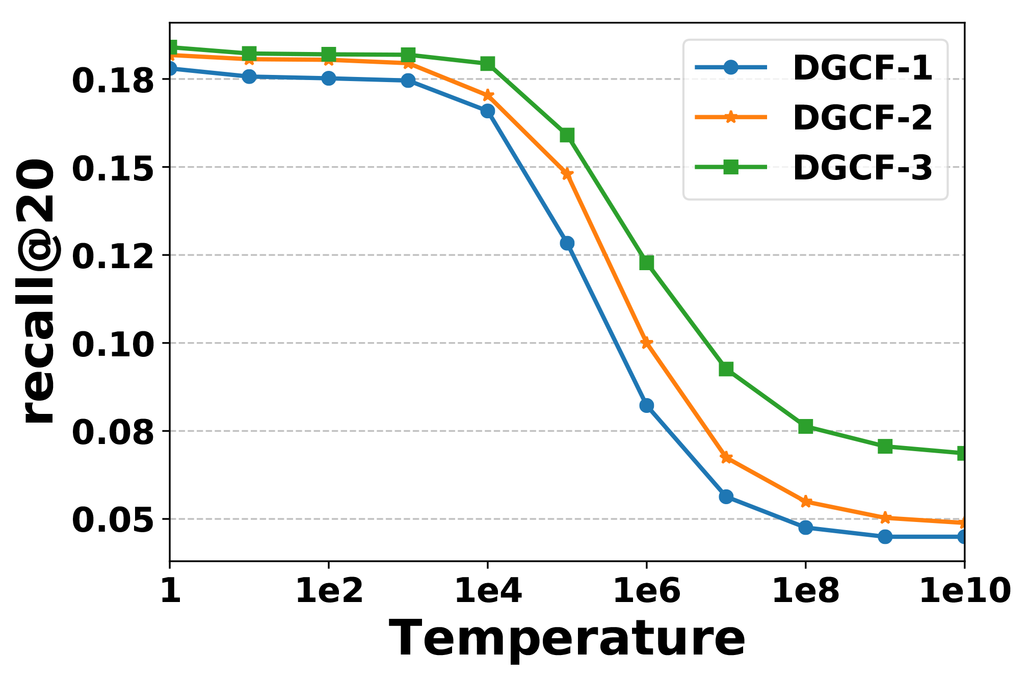
(a) Disentanglement w.r.t. recall.

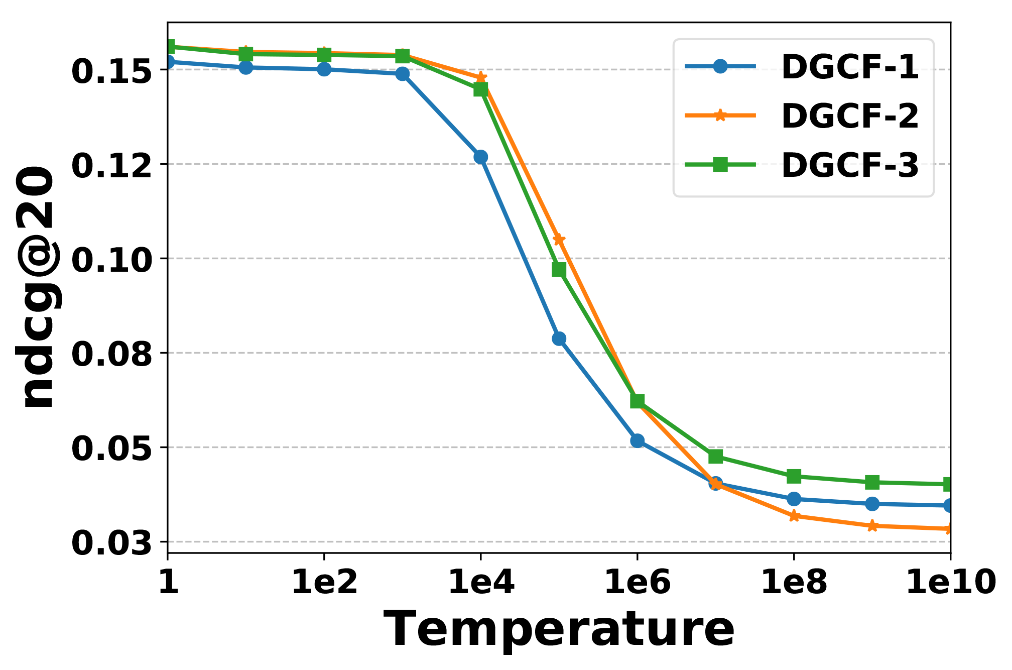
(b) Disentanglement w.r.t. ndcg.

Figure 6. Disentanglement of Intents. Best Viewed in Color.

4.3.3. Impact of Independence Modeling.

As introduced in Equation (14) distance correlation is a statistic measure to quantify the level of independence, we hence select MF, NGCF, and DGCF to separately represent three fashions to model user-item relationships — isolated data instance, holistic interaction graph, and intent-aware interaction graphs, respectively. We report the result comparison w.r.t. distance correlation in Table 4. Furthermore, conduct another ablation study to verify the influence of independence modeling. To be more specific, we disable this module in DGCF-1, DGCF-2, and DGCF-3 to separately build the variants DGCF-1${}_{\text{ind}}$, DGCF-2${}_{\text{ind}}$, and DGCF-3${}_{\text{ind}}$. We show the results in Table 5. There are some observations:

• A better performance is substantially coupled with a higher level of independence across the board. In particular, focusing on one model group, the intents of DGCF${}_{\text{ind}}$ are more highly entangled than that of DGCF; meanwhile, DGCF is superior to its variants w.r.t. recall in Gowalla and Yelp2018 datasets. This reflects the correlation between the performance and disentanglement, which is consistent to the observation in (Ma et al., 2019b).

• When analyzing the comparison across model groups, we find that the performance drop caused by removing the independence modeling from DGCF-2 is more obvious in DGCF-1. This suggests that the independence regularizer is more beneficial to the deeper models, leading to better intent-aware representations.

4.4. In-depth Analysis (RQ3)

In what follows, we conduct experiments to get deep insights into the disentangled representations w.r.t. the disentanglement of intents and interpretability of representations.

4.4.1. Disentanglement of Intents.

Disentangled representation learning aims to generate factorial representations, where a change in one factor is relatively invariant to changes in other factors (Bengio et al., 2013). We hence investigate whether the intent-aware representations of DGCF match this requirement well, and get deep insights into the disentanglement. Towards this end, we introduce a temperature factor, $\tau$, into the graph disentangling module. Specifically, for each user/item factorial representation, we first select a particular intent $k$, whose $A_{k}(u,i)$ is the smallest in $K$ intents, and then use $\tau$ to reassign it with a smaller weight $\frac{A_{k}(u,i)}{\tau}$, while remaining the other intents unchanged. Wherein, $\tau$ is searched in the range of $\{10^{0},10^{1},10^{2},\cdots,10^{10}\}$. Through this way, we study its influence on recommendation performance. The results in Gowalla dataset is shown in Figure 6. We have several interesting observations:

• The discovered intents serve as vitamin to the disentangled representations. That is, even the intents in small quantities (i.e., when $\tau$ ranges from $10^{0}$ to $10^{3}$) are beneficial to the representation learning. This also verifies the independence of intents: the changes on the specific intent almost have no influence on the others, still leading to comparable performances to the optimal one.

• The vitamin also means that the deficiency of any intent hinders the results severely. When $\tau$ is larger than $10^{4}$, the performance drops quickly, which indicates that lack of intents (whose influences is close to zero) negatively affects the model. Moreover, this verifies that one intent cannot be inferred by the others.

4.4.2. Interpretability of Representations.

We now explore the semantics of the explored intents. Towards this end, in Yelp2018^∗ datasets, we use side information (i.e., user reviews) which possibly contain some cues for why users visit the local business (i.e., self-generated explanations on their behaviors). In particular, we randomly selected two users $u_{10362}$ and $u_{10360}$, and disentangled the explored intents behind each historical user-item interactions, based on the learned intent-aware graphs. Thereafter, for each interaction, we coupled its review with the intent with the highest confidence score. For example, conditioned on the intent $k_{1}$, interaction $(u_{10360},i_{11732})$ has the hightest score $0.313$ among $u_{10362}$’s history. Figure 5 shows the post-hoc explanations of intents, and we have the following findings:

• Jointly analyzing reviews for the same intent, we find that, while showing different fine-grained preferences, they are consistent with some high-level concepts. For example, intent $k_{1}$ contributes the most to interactions $(u_{10362},i_{88})$ and $(u_{10360},i_{11732})$, which suggests its high confidence of being the intents behind these behaviors. We hence analyze the reviews of interactions, and find that they are about users’ special interests: the late 90s for $u_{10362}$, and hospital gown for $u_{10360}$.

• DGCF is able to discover user intents inherent in historical behaviors. Examining the corresponding reviews, we summarize the semantics (high-level concept) of these four intents $k_{1}$, $k_{2}$, $k_{3}$, and $k_{4}$ as interesting matching, service, price&promotion, and passing the time, respectively. This verifies the rationality of our assumptions: user behaviors are driven by multiple intents with varying contributions.

• This inspires us to go beyond user-item interactions and consider extra information to model user intents in an explicit fashion. We plan to incorporate psychology knowledge in future work.

5. Conclusion And Future Work

In this work, we exhibited user-item relationships at the granularity of user intents and disentangled these intents in the representations of users and items. We devised a new framework, DGCF, which utilizes the graph disentangling module to iteratively refine the intent-aware interaction graphs and factorial representations. We further introduce the independence modeling module to encourage the disentanglement. We offer deep insights into the DGCF w.r.t. effectiveness of recommendation, disentanglement of user intents, and interpretability of factorial representations.

Learning disentangled user intents is an effective solution to exploit diverse relationships among users and items, and also helps greatly to interpret their representations. This work shows initial attempts towards interpretable recommender models. In future work, we will involve side information, such as conversation history with users (Lei et al., 2020), item knowledge (Wang et al., 2019c, a, 2020; Sun et al., 2020; Hong et al., 2017), and user reviews (Li et al., 2019; Cheng et al., 2018), or conduct psychology experiments (Lu et al., 2019) to establish the ground truth on user intents and further interpret disentangled representations better. Furthermore, we would like to explore the privacy and robustness of the factorial representations, with the target of avoiding the leakage of sensitive information.

- (1)
- Belghazi et al. (2018) Mohamed Ishmael Belghazi, Aristide Baratin, Sai Rajeswar, Sherjil Ozair, Yoshua Bengio, R. Devon Hjelm, and Aaron C. Courville. 2018. Mutual Information Neural Estimation. In ICML. 530–539.
- Bengio et al. (2013) Yoshua Bengio, Aaron C. Courville, and Pascal Vincent. 2013. Representation Learning: A Review and New Perspectives. PAMI 35, 8 (2013), 1798–1828.
- Chen et al. (2017) Jingyuan Chen, Hanwang Zhang, Xiangnan He, Liqiang Nie, Wei Liu, and Tat-Seng Chua. 2017. Attentive Collaborative Filtering: Multimedia Recommendation with Item- and Component-Level Attention. In SIGIR. 335–344.
- Chen et al. (2019) Tong Chen, Hongzhi Yin, Hongxu Chen, Rui Yan, Quoc Viet Hung Nguyen, and Xue Li. 2019. AIR: Attentional Intention-Aware Recommender Systems. In ICDE. 304–315.
- Cheng et al. (2018) Zhiyong Cheng, Ying Ding, Lei Zhu, and Mohan S. Kankanhalli. 2018. Aspect-Aware Latent Factor Model: Rating Prediction with Ratings and Reviews. In WWW. 639–648.
- Du et al. (2018) Chao Du, Chongxuan Li, Yin Zheng, Jun Zhu, and Bo Zhang. 2018. Collaborative Filtering With User-Item Co-Autoregressive Models. In AAAI. 2175–2182.
- Ebesu et al. (2018) Travis Ebesu, Bin Shen, and Yi Fang. 2018. Collaborative Memory Network for Recommendation Systems. In SIGIR. 515–524.
- Glorot and Bengio (2010) Xavier Glorot and Yoshua Bengio. 2010. Understanding the difficulty of training deep feedforward neural networks. In AISTATS. 249–256.
- Hamilton et al. (2017) William L. Hamilton, Zhitao Ying, and Jure Leskovec. 2017. Inductive Representation Learning on Large Graphs. In NeurIPS. 1025–1035.
- He et al. (2020) Xiangnan He, Kuan Deng, Xiang Wang, Yan Li, Yongdong Zhang, and Meng Wang. 2020. LightGCN: Simplifying and Powering Graph Convolution Network for Recommendation. In SIGIR.
- He et al. (2018) Xiangnan He, Zhankui He, Jingkuan Song, Zhenguang Liu, Yu-Gang Jiang, and Tat-Seng Chua. 2018. NAIS: Neural Attentive Item Similarity Model for Recommendation. TKDE 30, 12 (2018), 2354–2366.
- He et al. (2017) Xiangnan He, Lizi Liao, Hanwang Zhang, Liqiang Nie, Xia Hu, and Tat-Seng Chua. 2017. Neural Collaborative Filtering. In WWW. 173–182.
- Higgins et al. (2017) Irina Higgins, Loïc Matthey, Arka Pal, Christopher Burgess, Xavier Glorot, Matthew Botvinick, Shakir Mohamed, and Alexander Lerchner. 2017. beta-VAE: Learning Basic Visual Concepts with a Constrained Variational Framework. In ICLR.
- Hinton et al. (2011) Geoffrey E. Hinton, Alex Krizhevsky, and Sida D. Wang. 2011. Transforming Auto-Encoders. In ICANN. 44–51.
- Hong et al. (2017) Richang Hong, Lei Li, Junjie Cai, Dapeng Tao, Meng Wang, and Qi Tian. 2017. Coherent Semantic-Visual Indexing for Large-Scale Image Retrieval in the Cloud. TIP 26, 9 (2017), 4128–4138.
- Kabbur et al. (2013) Santosh Kabbur, Xia Ning, and George Karypis. 2013. FISM: factored item similarity models for top-N recommender systems. In KDD. 659–667.
- Kingma and Ba (2015) Diederik P. Kingma and Jimmy Ba. 2015. Adam: A Method for Stochastic Optimization. In ICLR.
- Kipf and Welling (2017) Thomas N. Kipf and Max Welling. 2017. Semi-Supervised Classification with Graph Convolutional Networks. In ICLR.
- Koren (2008) Yehuda Koren. 2008. Factorization meets the neighborhood: a multifaceted collaborative filtering model. In KDD. 426–434.
- Koren et al. (2009) Yehuda Koren, Robert M. Bell, and Chris Volinsky. 2009. Matrix Factorization Techniques for Recommender Systems. IEEE Computer 42, 8 (2009), 30–37.
- Lei et al. (2020) Wenqiang Lei, Xiangnan He, Yisong Miao, Qingyun Wu, Richang Hong, Min-Yen Kan, and Tat-Seng Chua. 2020. Estimation-Action-Reflection: Towards Deep Interaction Between Conversational and Recommender Systems. In WSDM. 304–312.
- Li et al. (2019) Chenliang Li, Cong Quan, Li Peng, Yunwei Qi, Yuming Deng, and Libing Wu. 2019. A Capsule Network for Recommendation and Explaining What You Like and Dislike. In SIGIR. 275–284.
- Liang et al. (2018) Dawen Liang, Rahul G. Krishnan, Matthew D. Hoffman, and Tony Jebara. 2018. Variational Autoencoders for Collaborative Filtering. In WWW. 689–698.
- Lu et al. (2019) Hongyu Lu, Min Zhang, Weizhi Ma, Yunqiu Shao, Yiqun Liu, and Shaoping Ma. 2019. Quality effects on user preferences and behaviorsin mobile news streaming. In WWW. 1187–1197.
- Ma et al. (2019a) Jianxin Ma, Peng Cui, Kun Kuang, Xin Wang, and Wenwu Zhu. 2019a. Disentangled Graph Convolutional Networks. In ICML. 4212–4221.
- Ma et al. (2019b) Jianxin Ma, Chang Zhou, Peng Cui, Hongxia Yang, and Wenwu Zhu. 2019b. Learning Disentangled Representations for Recommendation. In NeurIPS. 5712–5723.
- Rao et al. (2015) Nikhil Rao, Hsiang-Fu Yu, Pradeep Ravikumar, and Inderjit S. Dhillon. 2015. Collaborative Filtering with Graph Information: Consistency and Scalable Methods. In NeurIPS. 2107–2115.
- Rendle et al. (2009) Steffen Rendle, Christoph Freudenthaler, Zeno Gantner, and Lars Schmidt-Thieme. 2009. BPR: Bayesian Personalized Ranking from Implicit Feedback. In UAI. 452–461.
- Sabour et al. (2017) Sara Sabour, Nicholas Frosst, and Geoffrey E. Hinton. 2017. Dynamic Routing Between Capsules. In NeurIPS. 3856–3866.
- Salakhutdinov et al. (2007) Ruslan Salakhutdinov, Andriy Mnih, and Geoffrey E. Hinton. 2007. Restricted Boltzmann machines for collaborative filtering. In ICML. 791–798.
- Sedhain et al. (2015) Suvash Sedhain, Aditya Krishna Menon, Scott Sanner, and Lexing Xie. 2015. AutoRec: Autoencoders Meet Collaborative Filtering. In WWW. 111–112.
- Sun et al. (2020) Changfeng Sun, Han Liu, Meng Liu, Zhaochun Ren, Tian Gan, and Liqiang Nie. 2020. LARA: Attribute-to-Feature Adversarial Learning for New-Item Recommendation. In WSDM. 582–590.
- Székely et al. (2009) Gábor J Székely, Maria L Rizzo, et al. 2009. Brownian distance covariance. The annals of applied statistics 3, 4 (2009), 1236–1265.
- Székely et al. (2007) Gábor J Székely, Maria L Rizzo, Nail K Bakirov, et al. 2007. Measuring and testing dependence by correlation of distances. The annals of statistics 35, 6 (2007), 2769–2794.
- Tay et al. (2018) Yi Tay, Luu Anh Tuan, and Siu Cheung Hui. 2018. Latent Relational Metric Learning via Memory-based Attention for Collaborative Ranking. In WWW. 729–739.
- van den Berg et al. (2017) Rianne van den Berg, Thomas N. Kipf, and Max Welling. 2017. Graph Convolutional Matrix Completion. In KDD.
- Vaswani et al. (2017) Ashish Vaswani, Noam Shazeer, Niki Parmar, Jakob Uszkoreit, Llion Jones, Aidan N. Gomez, Lukasz Kaiser, and Illia Polosukhin. 2017. Attention is All you Need. In NeurIPS. 5998–6008.
- Velickovic et al. (2018) Petar Velickovic, Guillem Cucurull, Arantxa Casanova, Adriana Romero, Pietro Liò, and Yoshua Bengio. 2018. Graph Attention Networks. In ICLR.
- Wang et al. (2019a) Xiang Wang, Xiangnan He, Yixin Cao, Meng Liu, and Tat-Seng Chua. 2019a. KGAT: Knowledge Graph Attention Network for Recommendation. In KDD. 950–958.
- Wang et al. (2019b) Xiang Wang, Xiangnan He, Meng Wang, Fuli Feng, and Tat-Seng Chua. 2019b. Neural Graph Collaborative Filtering. In SIGIR.
- Wang et al. (2019c) Xiang Wang, Dingxian Wang, Canran Xu, Xiangnan He, Yixin Cao, and Tat-Seng Chua. 2019c. Explainable Reasoning over Knowledge Graphs for Recommendation. In AAAI.
- Wang et al. (2020) Xiang Wang, Yaokun Xu, Xiangnan He, Yixin Cao, Meng Wang, and Tat-Seng Chua. 2020. Reinforced Negative Sampling over Knowledge Graph for Recommendation. In WWW. 99–109.
- Wu et al. (2019) Felix Wu, Amauri H. Souza Jr., Tianyi Zhang, Christopher Fifty, Tao Yu, and Kilian Q. Weinberger. 2019. Simplifying Graph Convolutional Networks. In ICML. 6861–6871.
- Wu et al. (2016) Yao Wu, Christopher DuBois, Alice X. Zheng, and Martin Ester. 2016. Collaborative Denoising Auto-Encoders for Top-N Recommender Systems. In WSDM. 153–162.
- Yang et al. (2018) Jheng-Hong Yang, Chih-Ming Chen, Chuan-Ju Wang, and Ming-Feng Tsai. 2018. HOP-rec: high-order proximity for implicit recommendation. In RecSys. 140–144.
- Ying et al. (2018) Rex Ying, Ruining He, Kaifeng Chen, Pong Eksombatchai, William L. Hamilton, and Jure Leskovec. 2018. Graph Convolutional Neural Networks for Web-Scale Recommender Systems. In KDD. 974–983.
- Ying et al. (2019) Zhitao Ying, Dylan Bourgeois, Jiaxuan You, Marinka Zitnik, and Jure Leskovec. 2019. Gnnexplainer: Generating explanations for graph neural networks. In NeurIPS. 9240–9251.