Topology Optimization of Two Fluid Heat Exchangers

Abstract

A method for density-based topology optimization of heat exchangers with two fluids is proposed. The goal of the optimization process is to maximize the heat transfer from one fluid to the other, under maximum pressure drop constraints for each of the fluid flows. A single design variable is used to describe the physical fields. The solid interface and the fluid domains are generated using an erosion-dilation based identification technique, which guarantees well-separated fluids, as well as a minimum wall thickness between them. Under the assumption of laminar steady flow, the two fluids are modelled separately, but in the entire computational domain using the Brinkman penalization technique for ensuring negligible velocities outside of the respective fluid subdomains. The heat transfer is modelled using the convection-diffusion equation, where the convection is driven by both fluid flows. A stabilized finite element discretization is used to solve the governing equations. Results are presented for two different problems: a two-dimensional example illustrating and verifying the methodology; and a three-dimensional example inspired by shell-and-tube heat exchangers. The optimized designs for both cases show an improved heat transfer compared to the baseline designs. For the shell-and-tube case, the full freedom topology optimization approach is shown to yield performance improvements of up to 113% under the same pressure drop.

1 Introduction

Heat exchangers are devices that serve to transfer thermal energy between two or more fluids, usually separated by solid walls to avoid mixing. They can be used for both cooling and heating applications, with some of the most well-known being in combustion engine cooling, air conditioning, power production and refrigeration.

Heat exchangers are widely used and their analysis is covered in most basic heat transfer courses and any good book on heat transfer, e.g. [1]. They are typically dimensioned and designed based on classical heat transfer theory under certain assumptions for predefined geometric layouts [2] . In recent time, the use of computational fluid dynamics (CFD) and conjugate heat transfer (CHT) simulations has become an indispensable tool for the analysis and design of complex heat exchangers [3]. However, their designs are still mainly restricted to the classical, and rather simple, geometries, such as parallel flow, counter-flow and cross-flow heat exchangers, as illustrated in Figure 1. These can be assembled from standard components and manufacturing processes, e.g. punching and brazing, ensuring easy mass production at low cost.

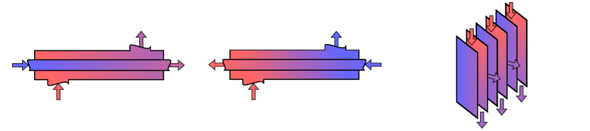
Figure 1: Illustration of common heat exchanger configurations. From left: Parallel flow, counter-flow and cross-flow heat exchangers.

Recent advances within additive manufacturing of conductive metals have spurred an increase in the internal geometric complexity of new heat exchanger designs [4, 5]. However, emphasis is put on maximizing the internal interacting surface area, using for instance Triply Periodic Minimal Surfaces (TPMS) [5]. This relies on a critical assumption based on Newton’s law of cooling for the heat flux due to convection $q_{\text{conv}}=h\,A_{s}(T_{s}-T_{\infty})$, where $h$ is the convection heat transfer coefficient, $A_{s}$ is the area of the heat transfer surface, $T_{s}$ is the temperature of the surface and $T_{\infty}$ is the fluid reference temperature. It seems obvious to increase the surface area, $A_{s}$, to increase the heat flux. But an increase in the surface area due to increasing geometric complexity almost certainly leads to a decrease in the convection coefficient, $h$, since the fluids will flow slower due to a higher flow resistance. Of course, one can always use a more powerful pump to circumvent this, but the increased energy input must be weighted by the overall efficiency of the heat exchanger. Therefore, this paper proposes a novel approach for the simulation-driven design optimization of pressure-drop-constrained two-fluid heat exchangers with a separating solid conductive wall using topology optimization. The approach optimizes the heat exchanger by a direct measure of the heat exchanger efficiency, based on simulations, rather than an implicit geometric quantity such as the surface area.

Topology optimization is a computational design methodology for optimizing structures. It originated in the field of solid mechanics [6] and has seen widespread use there [7] over the past three decades. As detailed in the recent review paper by Alexandersen and Andreasen [8], topology optimization has been applied to a wide range of flow-based problems since the first application to Stokes flow by Borrvall and Petersson [9] in 2003. In order to apply topology optimization to heat exchanger design, it is necessary to be able to treat three-dimensional problems with high mesh resolutions. The three-dimensionality is necessary to model the complex interactions of most heat exchangers and the high mesh resolution is mainly necessary to provide a high design freedom for topology optimization by resolving small features (e.g. thin solid walls). For large scale three-dimensional flow-based problems, previous works have treated pure fluid flow [10, 11, 12, 13, 14, 15, 16] and conjugate heat transfer problems for forced convection [17, 18, 19, 20, 21, 22] and natural convection [23, 24, 25].

In the context of topology optimization, literature on the design of heat exchangers is very sparse. Two papers have treated guiding channels or winglets for fin-and-tube heat exchangers [26, 27]. However, they only consider additional flow guiding features for existing heat exchanger geometries. Only a few works consider the design of the actual heat exchanger solid surface geometry using topology optimization. The first is the M.Sc. thesis by Papazoglou [28] investigating both a fluid tracking model and a multi-fluid model for a density-based approach. The second is the Ph.D. thesis by Haertel [29] coupling two-dimensional in-plane and out-of-plane flow models using an interface model similar to our approach. The third is the paper by Tawk et al. [30] proposing a density-based multi-fluid approach for optimizing heat exchangers with two separate fluids and a solid. The fourth is the conference paper by Saviers et al. [31] which, however, provides very little technical details on the applied methodology. Finally, very recently, after the completion of the present work, a preprint was uploaded to arXiv.org by Kobayashi et al. [32]. The authors also use a single design variable to parametrize two fluids and a solid. The solid is represented by intermediate design variable values, whose existence is guaranteed due to filtering of the design field. However, the approach does not appear to have thickness control of the solid and is only applied to smaller computational problems.

Interface identification techniques are used to capture the transition from one physical phase to another. Such a technique was introduced by Clausen et al. [33, 34] for topology optimization of coated structures. The method uses the spatial gradient of the design variable to identify where coating should be applied. More recently, a modified formulation was introduced by Luo et al. [35], where the design field is eroded and dilated, with the intersection of these fields identifying the interface.

The paper is organized as follows: Section 2 introduces the parametrization and states the goal and constraint of the optimization problem; Section 3 details the physics of the problem and the assumptions made; Section 4 provides an brief description of the finite element formulation; Section 5 presents the proposed topology optimization methodology; Section 6 show optimized heat exchangers for two numerical examples; and Section 7 provides a discussion and conclusions.

2 Parametrization

The goal of the optimization problem is to maximize the heat transferred in a heat exchanger at a given operational power, which is proportional to the pressure drop across the heat exchanger.

The problem concerns the arrangement of a solid interface, which separates the two fluids, as illustrated in Figure 2. The fluid domains are denoted $\Omega^{\gamma}$, where superscript $\gamma$ is the fluid index, and are separated by a solid domain $\Omega^{s}$. The total computational domain is given as the union of all subdomains, $\Omega=\Omega^{1}\cup\Omega^{2}\cup\Omega^{s}$. In order to introduce the design representation the non-overlapping domain representation is relaxed, such that both fluids may be present in the entire domain. However, by the use of an identification technique, every point in the domain is sought to be exclusively assigned either as one of the two fluids or as solid. This means that the velocity of a fluid should be zero outside of its domain $\Omega^{\gamma}$.

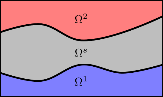
Figure 2: Sketch of the subdomains in the domain of interest. The $\Omega^{1}$ (blue) and $\Omega^{2}$ (red) domains are the domains of fluids 1 and 2, respectively. The solid domain, $\Omega^{s}$ (grey), separates the two fluids.

3 Governing equations

A two fluid heat exchanger contains two mass transfer problems (one for each fluid) and one global heat transfer problem. The governing equations are derived under the assumption of steady state, constant fluid properties and incompressibility. Furthermore, heat generated by viscous dissipation is neglected. The stated assumptions result in a weak coupling between the mass and heat transfer, as only the mass transfer affects the heat transfer, but not the other way around.

In the following, the governing equations are presented in their dimensionless form.

3.1 Mass transfer

The mass transfer for each of the fluid domains is obtained by solving the dimensionless Navier-Stokes equations. The equations for each mass transfer are posed in the entire domain $\Omega$ to permit topology optimization. A Brinkman friction term is used to penalize fluid flow outside the fluid subdomain [9, 36, 37].

For each fluid, denoted by index $\gamma$ the non-dimensional equations yield:

$$u_{i}^{\gamma}\frac{\partial u_{j}^{\gamma}}{\partial x_{i}}-\frac{1}{\mathit{Re}^{\gamma}}\frac{\partial}{\partial x_{i}}\left(\frac{\partial u_{i}^{\gamma}}{\partial x_{j}}+\frac{\partial u_{j}^{\gamma}}{\partial x_{i}}\right)+\frac{\partial P^{\gamma}}{\partial x_{i}} =-\alpha^{\gamma}(\mathbf{x})u_{i}^{\gamma}$$ (1)

$$\frac{\partial u_{i}^{\gamma}}{\partial x_{i}} =0$$ (2)

where $u$ is velocity, $P$ the dynamic pressure and $\alpha$ the impermeability. The Reynolds number, $\mathit{Re}$, is a dimensionless parameter indicating the ratio between the inertial and the viscous forces in the flow. It is expressed as a function of a reference velocity, $U$, a length scale $L$, the fluid mass density $\rho$ and dynamic viscosity $\mu$:

$$\mathit{Re}=\frac{UL\rho}{\mu}$$ (3)

The impermeability, $\alpha(\mathbf{x})$, is defined for each point in the domain:

$$\alpha^{\gamma}(\mathbf{x})=\left\{\begin{array}[]{ll}0&{\rm if}\;\mathbf{x}\in\Omega^{\gamma}\\ \infty&{\rm if}\;\mathbf{x}\notin\Omega^{\gamma}\end{array}\right.$$ (4)

where it is seen that the impermeability is always $\alpha^{\gamma}=\infty$ outside of fluid $\gamma$. In practice, the impermeability can not be set to $\alpha=\infty$ for numerical reasons. Instead, a large value is used. For consistency, the impermeability outside of the fluid region is related to the Darcy number [38] and is given as:

$$\overline{\alpha}^{\gamma}=\frac{1}{\mathit{Re}^{\gamma}}\frac{1}{\mathit{Da}}$$ (5)

The mass transfer problems are subject to homogeneous Dirichlet boundary conditions on the velocity at the domain boundaries, not being in- or outlets. A homogeneous Dirichlet boundary condition is placed on the pressure at the outlet.

3.2 Heat transfer

The heat transfer is described by the convection-diffusion equation. The equation is non-dimensionalised using the solid conductivity, $k^{s}$. As the velocities are assumed to be $u_{i}^{\gamma}=0$ outside of their respective corresponding domain $\Omega^{\gamma}$, the heat transfer in the entire computational domain $\Omega$ can be expressed as:

$$\sum_{\gamma=1}^{\mathit{NF}}\left(\mathit{Pe}_{s}^{\gamma}u_{i}^{\gamma}\right)\frac{\partial T}{\partial x_{i}}-\frac{\partial}{\partial x_{i}}\left(C_{k}(\mathbf{x})\frac{\partial T}{\partial x_{i}}\right)=0$$ (6)

where $\mathit{Pe}_{s}^{\gamma}$ is the solid Peclet number, which relates the convective heat transfer in a fluid to the diffusive heat transfer in the solid. The conductivity ratio, $C_{k}^{\gamma}$, is the fluid conductivity normalized by the solid conductivity. These parameters can be linked to the conventional Peclet number of each fluid:

$$\mathit{Pe}_{s}^{\gamma} =\frac{\rho^{\gamma}c_{p}^{\gamma}UL}{k^{s}} C_{k}^{\gamma} =\frac{k^{\gamma}}{k^{s}} \mathit{Pe}^{\gamma} =\frac{\mathit{Pe}_{s}^{\gamma}}{C_{k}^{\gamma}}$$ , , (7)

The heat transfer problem is modelled by one equation for the entire domain $\Omega$, with a spatially varying coefficient $C_{k}$ defined by:

$$C_{k}(\mathbf{x})=\left\{\begin{array}[]{ll}C_{k}^{\gamma}&{\rm if}\;\mathbf{x}\in\Omega^{\gamma}\\ 1&{\rm if}\;\mathbf{x}\in\Omega^{s}\end{array}\right.$$ (8)

The boundary conditions for the heat transfer problem consist of Dirichlet boundary conditions at the respective fluid inlets. On the rest of the domain boundary, a homogeneous Neumann boundary condition is imposed, resulting in the design domain being externally insulated.

4 Finite element formulation

The equation system is discretized and solved using the Finite Element Method (FEM), using structured meshes with regular trilinear hexahedral elements. PSPG stabilization is employed to facilitate the use of equal-order elements. SUPG stabilization is applied to both mass transfer problems and the heat transfer problem to alleviate problems with steep gradients due to convection. The implementation from [23] is reused here without the Boussinesq approximation terms. As the coupling between the mass and heat transfer considered here is weak, the problems are solved sequentially.

The two mass transfer problems are solved by finding the solution to the vector of residual equations given by:

$$\mathbf{R}_{\mathit{F\gamma}}=\mathbf{M}\left(\mathbf{u}_{\mathit{F\gamma}},\bm{\alpha}_{\gamma}\right)\mathbf{u}_{\mathit{F\gamma}}-\mathbf{b}_{\mathit{F\gamma}}=\mathbf{0}$$ (9)

The solution vector $\mathbf{u}_{\mathit{F\gamma}}$ contains all three velocity components and the pressure for every node. The system matrix $\mathbf{M}\left(\mathbf{u}_{\mathit{F\gamma}},\bm{\alpha}_{\gamma}\right)$ contains the viscosity, convection, Brinkman penalization, pressure coupling and velocity divergence contributions, as well as all the corresponding SUPG and PSPG stabilization terms. The weak form and stabilization parameters are detailed in A.1.

Similarly, the residual equations for the heat transfer problem are defined as:

$$\mathbf{R}_{T}=\mathbf{M}_{T}\left(\mathbf{C_{k}},\,\mathbf{u}_{\mathit{Pe}}\right)\mathbf{T}-\mathbf{b}_{T}=\mathbf{0}$$ (10)

where the system is built based on the global velocity field combining both fluid flows:

$$\mathbf{u}_{\mathit{Pe}}=\mathit{Pe}_{s}^{1}\mathbf{u}_{\mathit{F1}}+\mathit{Pe}_{s}^{2}\mathbf{u}_{\mathit{F2}}$$ (11)

which is possible due to the assumption of the fluid domains being well-separated at the final design. The solution vector $\mathbf{T}$ contains the temperature in every node and the system matrix $\mathbf{M}_{T}\left(\mathbf{C_{k}},\,\mathbf{u}_{\mathit{Pe}}\right)$, is assembled from the thermal diffusion, convection and SUPG stabilization contributions. The weak form of these contributions, as well as the stabilization parameter, are detailed in A.2.

5 Topology optimization

5.1 Optimization problem

The generic optimization problem is given as the minimization of the objective function $\Phi$, subject to $m$ constraints $g_{i}$. Furthermore, a nested formulation is used where the residuals of the mass- and heat transfer problems from (9) and (10), are assumed zero in each iteration. The design variable $\xi$ is relaxed from discrete $\xi\in\{0,\;1\}$ to continuous $\xi\in[0,\;1]$ and represented by $n$ elementwise constant scalars.

$$\begin{split}\min_{\xi\in\left[0,\;1\right]^{n}}\;&\Phi(\xi,\;u^{1},\;u^{2},\;T)\\ \mathrm{s.t.}\;&\mathbf{R}_{F\gamma}=0,\;\gamma=\{1;\,2\}\\ &\mathbf{R}_{T}=0\\ &g_{i}\leq 0,\;i=1\dots m\end{split}$$ (12)

The objective function for a heat exchanger is to maximize the thermal energy transferred from the hot to the cold fluid. This can be expressed as minimizing the difference between the enthalpy flowing out at the cooled and coolant fluid outlets:

$$\Phi=\frac{1}{\int_{\Gamma_{F2}}dA}\left(\mathit{Pe}_{s}^{1}\int_{\Gamma_{F1}}n_{i}u^{1}_{i}TdA-\mathit{Pe}_{s}^{2}\int_{\Gamma_{F2}}n_{i}u^{2}_{i}TdA\right)$$ (13)

This objective function has the advantage of being defined on both fluid outlets, which it is beneficial for the computation of the sensitivities, as both mass transfer adjoint problems will have a source term on their respective outlets. However, it can be difficult to associate physical meaning to it. Therefore, for comparison purposes, we introduce $\Phi_{\mathit{coolant}}$, which is an expression of the heat transferred to the coolant, normalized by the outlet area:

$$\Phi_{\mathit{coolant}}=\frac{\mathit{Pe}_{s}^{2}}{\int_{\Gamma_{F2}}dA}\int_{\Gamma_{F2}}n_{i}u^{2}_{i}TdA$$ (14)

where a higher value is preferred since it reflect the amount of heat transferred to the coolant from the other fluid.

In order to regularize the geometry, and impose restrictions on the pumping power, the pressure drop on each fluid phase is controlled. This is done by placing a pressure drop constraint on each of the fluids:

$$g_{\gamma}=\frac{1}{\Delta P_{max}^{\gamma}\int_{\Gamma_{in,\;F\gamma}}dA}\int_{\Gamma_{in,\;F\gamma}}P^{\gamma}dA-1$$ (15)

where $\Delta P_{\mathit{max}}^{\gamma}$ is the maximal admissible pressure drop on fluid $\gamma$.

The optimization problem is solved using the Method of Moving Asymptotes (MMA) [39], implemented in PETSc [40] using external move limits of $0.2$.

5.2 Filtering and projecting

In topology optimization, filtering techniques are used to prevent checkerboards and other unwanted effects from appearing in the obtained designs [41]. The PDE filter [42, 40] is here used to obtain a filtered design field $\hat{\xi}$:

$$-R^{2}\nabla^{2}\hat{\xi}+\hat{\xi} =\xi$$ (16)

$$R =\frac{r}{2\sqrt{3}}$$ (17)

where $r$ is the physical filter radius.

A smooth Heaviside projection [43] with threshold $\eta$ and sharpness $\beta$ is applied to the filtered variable, which leads to the projected field $\tilde{\xi}$:

$$\tilde{\xi}(\hat{\xi},\beta,\eta)=\frac{\tanh(\beta\eta)+\tanh(\beta(\hat{\xi}-\eta))}{\tanh(\beta\eta)+\tanh(\beta(1-\eta))}$$ (18)

In combination with the filter, the Heaviside projection, can be used to enforce a minimum length scale on the obtained structures [43] if multiple design realizations are considered.

5.3 Modelling solid interfaces

A single design variable, $\xi$, is used to model three physical phases: two fluids and one solid. In order to ensure strict separation between the two fluid phases, it is important that there always exists a solid wall between them. A method for the introduction of a third phase between two already existing ones, has been introduced for minimization of elastic compliance of coated structures [33, 34, 35]. In its original application, the purpose of this method is to introduce a coating of a specific thickness between the void and the solid. In the present case, solid is placed between two fluids and allows for rigorous control of the interface thickness.

As seen in Figure 3, the process consists of a filtering operation with filter radius $r_{\mathit{min}}$ and a projection using the threshold $\eta=0.5$. This is done to ensure a well-defined interface. The obtained variable $\tilde{\xi}$ is refiltered using the erosion radius $r_{e}$, leading to the re-filtered variable $\hat{\tilde{\xi}}$. Finally, the re-filtered variable $\hat{\tilde{\xi}}$ is projected at a low and a high threshold, $\left\{\underline{\eta},\;\overline{\eta}\right\}=0.5\pm\Delta\eta$, yielding intermediate variables $\hat{\tilde{\xi}}_{1}$ and $\hat{\tilde{\xi}}_{2}$, respectively. The eroded and dilated variables, indicate which physical phase is applicable in each element (where the dilated variable, $\hat{\tilde{\xi}}_{1}$ is mapped for consistency):

$$\left\{\begin{array}[]{ll}\text{Fluid 1:}&\;\xi_{1}=1-\hat{\tilde{\xi}}_{1}=1\\ \text{Fluid 2:}&\;\xi_{2}=\hat{\tilde{\xi}}_{2}=1\\ \text{Solid:}&\;\xi_{1}=\xi_{2}=0\end{array}\right.$$ (19)

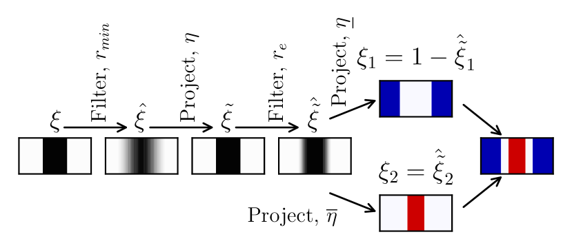
Figure 3: Overview of the different variables used in the erosion-dilation process. The resulting variables $\xi_{1}$ and $\xi_{2}$ are used to define the domains of the two fluids (red and blue) and of the solid interfaces (white).

Two advantages of the erosion-dilation technique should be mentioned here, one is that a separating solid phase is guaranteed between the two fluids and the other is that the thickness of this solid phase can be controlled. As shown by [35], a wall thickness $w_{e}$ is obtained by using the high and low threshold values and erosion filter radius:

$$\Delta\eta=0.45\qquad r_{e}\approx 0.75w_{e}$$ (20)

It is noted that the first filtering operation should have a filter radius larger than the wall thickness:

$$r_{\mathit{min}}>w_{e}$$ (21)

5.4 Interpolation functions

The relaxation of the optimization problem introduces the need for interpolation functions. Two parameters, the impermeabilities of both fluids $\alpha^{\gamma}$ and the conductivity ratio $C_{k}$ are interpolated from the variables obtained by the erosion-dilation process seen in Figure 3.

The impermeabilities $\alpha^{\gamma}$ are interpolated from the corresponding variable from the erosion-dilation process $\xi_{\gamma}$. The interpolation is done using RAMP [9, 44, 45]:

$$\alpha^{\gamma}(\xi_{\gamma})=\overline{\alpha}^{\gamma}\frac{1-\xi_{\gamma}}{1+\xi_{\gamma}q_{\alpha}}$$ (22)

where the upper limit $\overline{\alpha}^{\gamma}$ is the impermeability to be applied where the fluid $\gamma$ is not present, as discussed in Section 3.1. The parameter $q_{\alpha}$ indicates the curvature of the function, which is linear when $q_{\alpha}=0$.

The conductivity ratio $C_{k}$ for the heat transfer problem is interpolated from both $\xi_{1}$ and $\xi_{2}$. The interpolation has three bounds, such that Equation (8) is fulfilled. This is done by introducing the following interpolation function inspired by SIMP [46]:

$$C_{k}(\xi_{1},\;\xi_{2})=\left(1-\xi_{1}-\xi_{2}\right)^{p_{k}}+C_{k}^{1}\xi_{1}+C_{k}^{2}\xi_{2}$$ (23)

It is seen that the introduced interpolation function for $C_{k}$ has a penalization power $p_{k}$ on the solid phase, but not on the two terms corresponding to the fluid phases. Numerical studies concluded that this formulation circumvents high relative conductivities, when both $\xi_{1}$ and $\xi_{2}$ have intermediate values. In Figure 4, the interpolation function is shown for different penalization powers $p_{k}$.

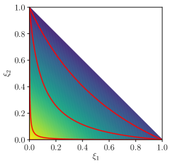
(a) $p_{k}=1$

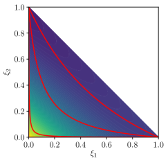
(b) $p_{k}=2$

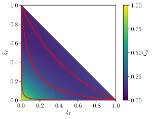
(c) $p_{k}=3$

Figure 4: Interpolation function for the relative conductivity, with $C_{k}^{1}=0.2$ and $C_{k}^{2}=0.1$. The red lines show the $\xi_{1}$ and $\xi_{2}$ combinations obtained with the identification method for $\beta=\left\{1,\;2,\;4\right\}$. Note that the northeastern part is white, as the corresponding combinations between $\xi_{1}$ and $\xi_{2}$ are not feasible.

5.5 Sensitivity analysis

The sensitivities of the objective and constraint functions are determined using the adjoint method. The method consists of setting up a Lagrangian function, where the residuals of the FEM problems are multiplied with the Lagrangian multipliers $\bm{\lambda}_{i}$ (also known as the adjoint variables):

$$\mathcal{L}=\Phi+\bm{\lambda}_{F1}^{\intercal}\mathbf{R}_{F1}+\bm{\lambda}_{F2}^{\intercal}\mathbf{R}_{F2}+\bm{\lambda}_{T}^{\intercal}\mathbf{R}_{T}$$ (24)

The derivative of the Lagrangian function is derived and rewritten using the chainrule, as seen in B.1, which results in the following sensitivity expression:

$$\frac{\mathrm{d}\Phi}{\mathrm{d}\xi}=\frac{\partial\Phi}{\partial\xi}+\bm{\lambda}_{T}^{\intercal}\frac{\partial\mathbf{R}_{T}}{\partial\xi}+\bm{\lambda}_{F1}^{\intercal}\frac{\partial\mathbf{R}_{F1}}{\partial\xi}+\bm{\lambda}_{F2}^{\intercal}\frac{\partial\mathbf{R}_{F2}}{\partial\xi}$$ (25)

where the Lagrangian multipliers are found by solving the three weakly coupled adjoint problems:

$$\left(\frac{\partial\mathbf{R}_{T}}{\partial T}\right)^{\intercal}\bm{\lambda}_{T} =\left(-\frac{\partial\Phi}{\partial T}\right)^{\intercal}$$ (26)

$$\left(\frac{\partial\mathbf{R}_{F1}}{\partial\mathbf{u_{1}}}\right)^{\intercal}\bm{\lambda}_{F1} =-\left[\left(\frac{\partial\Phi}{\partial\mathbf{u_{1}}}\right)^{\intercal}+\left(\frac{\partial\mathbf{R}_{T}}{\partial\mathbf{u_{1}}}\right)^{\intercal}\bm{\lambda}_{T}\right]$$ (27)

$$\left(\frac{\partial\mathbf{R}_{F2}}{\partial\mathbf{u_{2}}}\right)^{\intercal}\bm{\lambda}_{F2} =-\left[\left(\frac{\partial\Phi}{\partial\mathbf{u_{2}}}\right)^{\intercal}+\left(\frac{\partial\mathbf{R}_{T}}{\partial\mathbf{u_{2}}}\right)^{\intercal}\bm{\lambda}_{T}\right]$$ (28)

The transposed tangential system matrices used in the adjoint problem are, as in the physical problem, adjusted for the imposed Dirichlet boundary conditions on the physical problem. However, it should be noted, that all Dirichlet boundary conditions in the adjoint problems are homogeneous.

5.6 Continuation of parameters

The values of the projection sharpness, $\beta$, as well as the parameters of the interpolation functions, $q_{\alpha}$ and $p_{k}$ in (22) and (23), respectively, are to be set in order to obtain physical interpolation schemes. The initial parameters are chosen to give the optimizer a lot of freedom in the beginning, and modified to obtain sharper interfaces and a more accurate physical modelling as optimization progresses.

For two- and three-dimensional problems, a continuation step is applied every $40^{\text{th}}$ and $20^{\text{th}}$ design iteration, respectively, if the constraints have been met in the previous 3 iterations. Numerical studies showed that taking a single relaxation step on $q_{\alpha}$ performed well. When increasing the projection sharpens, the $\beta$ value is doubled. Finally, the penalization power for the relative conductivity interpolation, $p_{k}$, is increased simultaneously with the projection sharpness. The continuation scheme is shown in detail in Table 1.

Table 1: Projection sharpness and interpolation parameters as function of continuation step. Step 1 is the initial setting.

Step	$1$	$2$	$3$	$4$	$5$	$6$	$7$
$\beta$	$1$	$2$	$2$	$4$	$8$	$16$	$32$
$q_{\alpha}$	$10^{4}$	$10^{4}$	$10^{3}$	$10^{3}$	$10^{3}$	$10^{3}$	$10^{3}$
$p_{k}$	$1$	$1$	$1$	$2$	$2$	$3$	$3$

When starting with a higher projection sharpness than $\beta=1$, the scheme seen in Table 1 is used, replacing the $\beta$ value in step 1 and omitting the obsolete continuation steps.

6 Results

First, a simple optimization problem in two dimensions is considered. This relatively simple problem allows for a demonstration and verification of the methodology and the design representation by one design variable. Thereafter, a more complex three-dimensional problem is considered, where the full potential of the method is demonstrated.

6.1 Two-dimensional counter-flow heat exchanger

6.1.1 Problem definition

The first case considered is a two-dimensional counter-flow heat exchanger. The setup is seen in Figure 5 and consists of a hot fluid inlet in the lower-left part of the domain, with the corresponding outlet on the opposite lower-right side of the domain. A cold fluid inlet is located at the upper-right side of the domain, with the corresponding outlet at the opposite upper-left side. The inlets have parabolic velocity profiles assuming fully-developed laminar flow. Homogeneous Dirichlet boundary conditions are applied on the pressures at the respective outlets. Furthermore, a straight out velocity boundary condition is placed on the velocities at the outlets. The areas near the in- and outlets are excluded from the optimization to ensure undisturbed in- and outflow.

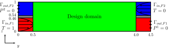
Figure 5: Sketch of the design domain for the two dimensional counter-flow heat exchanger. Green indicates the actual design domain, passive domains of the coolant- and cooled fluids are shown in blue and red, respectively. Grey indicates passive solid domains. The reference length is the height of the domain, $L=1$ and the reference velocity, the velocity at the inlet center, $U^{\gamma}=1$.

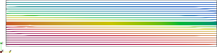
Figure 6: Baseline design of the two-dimensional counter-flow example. The two fluid phases consist of straight channels separated by a wall. Structure and streamlines are colored by temperature.

The problem presented here is optimized for computational Reynolds number $\mathit{Re}_{\mathit{comp}}^{\gamma}=100$, which leads to an actual Reynolds number $\mathit{Re}^{\gamma}=46$, for both fluids, when adjusted for their respective inlet sizes [23]. The reference velocity, $U$, is the maximum velocity, located at the center of the intlets. The computational Peclet number is $\mathit{Pe}_{\mathit{comp}}^{\gamma}=100$, as for the Reynolds numbers, this leads to the actual Peclet number $\mathit{Pe}^{\gamma}=46$.

Table 2: Computational parameters of heat exchanger

Property	Cooled	Coolant
Reynolds number $\scriptstyle\mathit{Re}[-]$	$100$	$100$
Solid Peclet number $\scriptstyle\mathit{Pe}_{s}[-]$	$4$	$4$
Conductivity ratio $\scriptstyle C_{k}[-]$	$0.04$	$0.04$
Impermeability $\scriptstyle\overline{\alpha}[-]$	$10^{4}$	$10^{4}$

The computational non-dimensional parameters are seen in Table 2. The optimization process is cut-off after a maximum of 500 design iterations.

The optimization problem is run with different maximum pressure drop constraints, which are obtained from the empty straight-channel design, as seen in Figure 6. The objective function is compared to the one from the same baseline design:

$$\Delta P^{\gamma}_{\mathit{base}}=1.57\qquad\Phi_{\mathit{coolant,\,base}}=0.856$$ (29)

6.1.2 Results

The problem is optimized for a range of values of admissible pressure drops $\Delta P_{\mathit{max}}$. It should be noted that the pressure drop in the channels cannot be smaller than the one from the baseline design, where the two channels are straight and parallel in the entire domain. The domain consists of $324\times 72\times 1$ cubic elements. The filter radii are set, such that the wall is $w_{e}=0.075$ thick, corresponding to $\approx 5$ elements. Furthermore, the filter radius has been set to $r_{\mathit{min}}=0.08$, as discussed in Section 5.3.

Two initial designs are considered in this example. The first one consists of the two parallel channels. In the second initial design, the entire design domain has been set to an intermediate design variable value, $\xi=0.5$, violating the strict separation of fluids.

A selection of the optimized structures, obtained at different admissible pressure drops and using the two initial designs are seen in Figure 7.

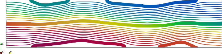
(a) $\Delta P_{\mathit{max}}=2.0\Delta P_{\mathit{base}}$, $\Phi_{\mathit{coolant}}=1.024$

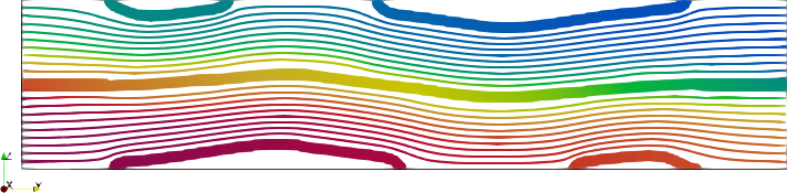
(b) $\Delta P_{\mathit{max}}=2.0\Delta P_{\mathit{base}}$, $\Phi_{\mathit{coolant}}=1.025$

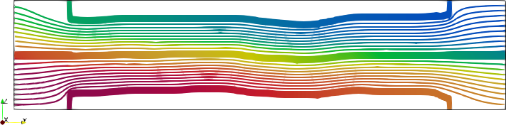
(c) $\Delta P_{\mathit{max}}=5.0\Delta P_{\mathit{base}}$, $\Phi_{\mathit{coolant}}=1.212$

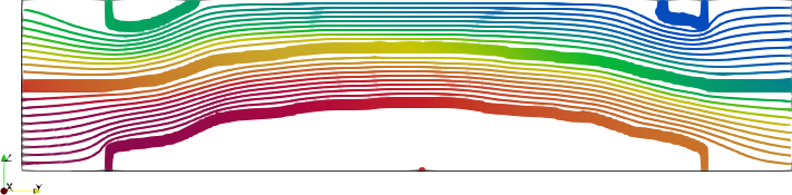
(d) $\Delta P_{\mathit{max}}=5.0\Delta P_{\mathit{base}}$, $\Phi_{\mathit{coolant}}=1.224$

(e) $\Delta P_{\mathit{max}}=10.0\Delta P_{\mathit{base}}$, $\Phi_{\mathit{coolant}}=1.395$

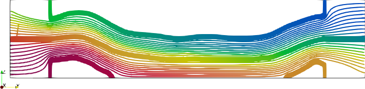
(f) $\Delta P_{\mathit{max}}=10.0\Delta P_{\mathit{base}}$, $\Phi_{\mathit{coolant}}=1.390$

Figure 7: Optimized structures and corresponding streamlines, colored by temperature. The structures are optimized with two different initial designs being, (a, c, e) the parallel channels and (b, d, f) $\xi=0.5$. The designs are optimized for different admissible pressure drops, (a, b) $\Delta P_{\mathit{max}}=2.0\Delta P_{\mathit{base}}$, (c, d) $\Delta P_{\mathit{max}}=5.0\Delta P_{\mathit{base}}$ and (e, f) $\Delta P_{\mathit{max}}=10.0\Delta P_{\mathit{base}}$. Structures are thresholded at $\alpha^{1}>0.1\overline{\alpha}^{1}\land\alpha^{2}>0.1\overline{\alpha}^{2}$.

With both initial designs, the channels get narrower, as the admissible pressure drop is increased. The narrower channels increase the flow speed of both fluids, which increases the heat transfer coefficient. Furthermore, in some cases, it is seen that the channels bend towards the domain boundary. A reason for this might be that a solid wall, with a high conductivity, can be avoided along the fluid. This wall might otherwise act as an unwanted regenerator.

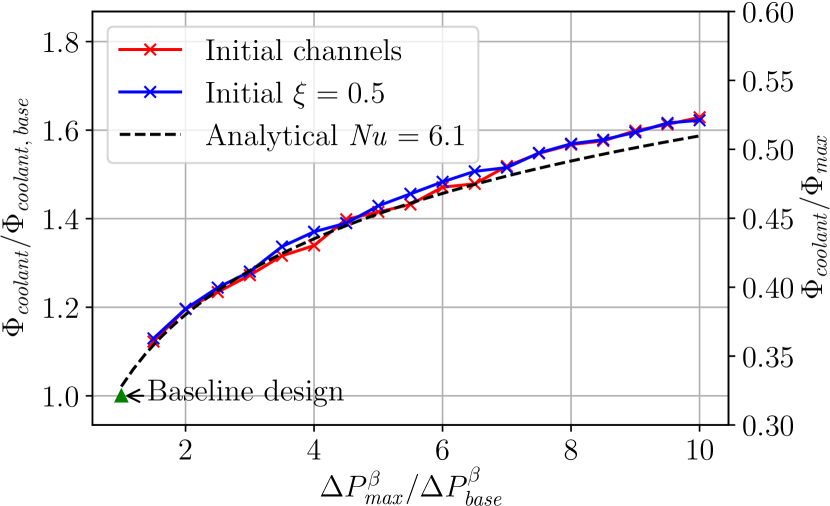
Figure 8: Improvement and fit of the transferred heat as a function of the admissible pressure drop in the fluids.

In Figure 7, a higher heat transfer is also observed for the designs optimized with a higher admissible pressure loss. In Figure 8, the heat transfer improvements (relative to the baseline design and to a theoretical limit) are compared for different admissible pressure drops (relative to the baseline design). The monitored improvement can be compared to a function of the admissible pressure drop $\Delta P_{\mathit{max}}$. This is done by noting the efficiency $\epsilon$ as a function of the Number of Transfer Units ($\mathit{NTU}$) [47]:

$$\epsilon =\frac{\Phi_{\mathit{coolant}}}{\Phi_{\mathit{max}}}=\frac{\mathit{NTU}}{1+\mathit{NTU}}$$ (30)

$$\mathit{NTU} =\frac{\mathit{UA}}{c_{p}\dot{m}}$$ (31)

where $\mathit{UA}$ is the overall heat transfer coefficient, which is dependent of the heat transfer coefficients $h_{F\gamma}$ of the two fluids:

$$\mathit{UA} =\left(\frac{L_{w}}{k_{w}A}+\frac{1}{h_{\mathit{F1}}A}+\frac{1}{h_{\mathit{F2}}A}\right)^{-1}$$ (32)

$$h_{F\gamma} =\frac{\mathit{Nu}_{\gamma}k_{F\gamma}}{D_{h}}$$ (33)

where $\mathit{Nu}_{\gamma}$ is the Nusselt number and $k_{\mathit{F\gamma}}$ the conductivity of the respective fluid. The Nusselt number for both fluids is found to be $\mathit{Nu}=6.1$ for this counter-flow heat exchanger problem. This was done by performing a numerical analysis of the baseline model in COMSOL. The hydraulic diameter is twice the height of the infinitely wide channel, $D_{h}=2w$, where $w$ is the channel height. Assuming all the pressure loss goes to making the channels narrower and that the flow is always fully developed, the width of the channel can be computed from integrating the volume flux of the Poiseuille flow:

$$\begin{split}V&=\int_{0}^{w}-\frac{1}{2\mu}\frac{dP}{dx}\left(yw-y^{2}\right)dz\\ \Rightarrow w&=w_{\mathit{base}}\sqrt[3]{\frac{\Delta P_{\mathit{base}}}{\Delta P}}\end{split}$$ (34)

Combining Equations (30-34), an analytical heat transfer enhancement for straight pipes with varying channel width $w$ can be computed and compared to the optimized designs. This is done assuming that the two fluids behave equally and that the allowable pressure drop is used exclusively to make the channels thinner on the entire length of the domain.

From Figure 8, it is seen that there is a very nice correspondence between the performance of the optimized designs and the theoretical prediction. At larger admissible pressure drops, the optimized designs outperform the theoretical prediction marginally. This confirms that, at least for this example, it is possible to obtain close to optimal designs using the presented methodology. The higher heat transfer by the designs obtained using the present methodology is due to the larger design freedom, which, for instance, makes the channels slightly curved. The slight advantage of these features can be seen from the two designs optimized for $\Delta P_{\mathit{max}}=5\Delta P_{\mathit{base}}$, where the design with the curved feature, Figure 7(d), slightly outperforms ($\sim 1\%$) the designs, where the channels have been narrowed, but stayed parallel, Figure 7(c).

Figure 9 shows the design field $\xi$ and the intermediate fields, obtained by optimizing with an admissible pressure drop $\Delta P_{\mathit{max}}=5\Delta P_{\mathit{base}}$ with the parallel channel initial design. From the eroded and dilated design fields, $\xi_{1}$ and $\xi_{2}$, seen in Figures 9(c) and 9(d), it is seen that the fields have the same features, but that they are eroded and dilated versions of Figure 9(b), which results in the wall. It is observed that the islands at the top and bottom of the computational domain are of the opposite fluid. This is also seen in Figure 10, where the fluid domains are shown for the optimized heat exchanger design. In Figure 9(g), the relative conductivity, $C_{k}$, in the design domain is shown. The walls are clearly identified with the higher conductivity. At the transition between the solid and the fluid, some few elements of intermediate conductivities are observed. However, this has very small influence on the final design, as very few elements are concerned.

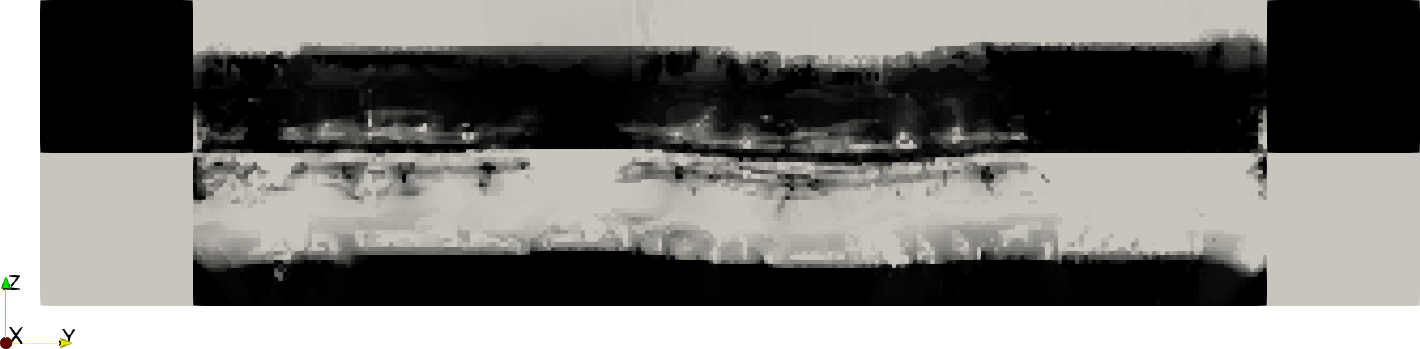
(a) $\xi$

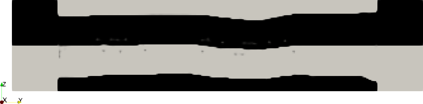
(b) $\hat{\tilde{\xi}}$

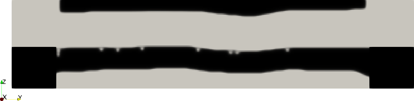
(c) $\xi_{1}$

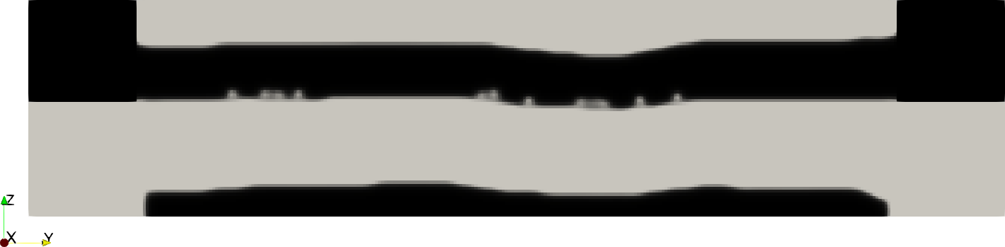
(d) $\xi_{2}$

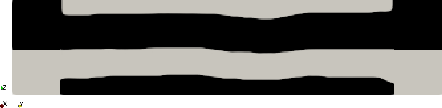
(e) $\alpha^{1}$

(f) $\alpha^{2}$

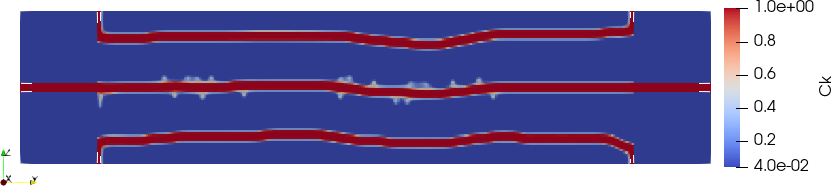
(g) $C_{k}$

Figure 9: Optimized fields, obtained by optimizing the parallel channels initial design, with a $\Delta P_{\mathit{max}}=5.0\Delta P_{\mathit{base}}$ pressure drop constraint. The design field $\xi$ (a) is filtered and projected to the filtered and projected field $\hat{\xi}$ (b). The erosion-dilation process, discussed in Section 5.3, is then used to generate $\xi_{1}$ (c) and $\xi_{2}$ (d), where the black region indicates the presence of the respective fluid. These fields lead to the physical fields (e-g), interpolated as discussed in Section 5.4.

Figure 10: Overview of the fluid domains in the design optimized for $\Delta P_{\mathit{max}}=5.0\Delta P_{\mathit{base}}$, with the parallel channels initial design. Red color denotes fluid 1, blue color fluid 2, and white the solid interface separating the two fluids.

In order to illustrate the distribution of the physical fields $\alpha^{\gamma}$ and $C_{k}$ along with their effect on the velocities and temperature, these quantities are probed along the vertical centerline in the baseline design seen in Figure 6 and in the design optimized with the baseline used as initial design and $\Delta P_{\mathit{max}}=5\Delta P_{\mathit{base}}$, seen in Figure 7(c). The probes are seen in Figure 11. In both cases, the wall is identified by the high relative conductivity and impermeabilities, as well as the low temperature gradient, caused by the high conductivities in the wall. In the probe of the optimized design, Figure 11(b), the islands of fluid are again highlighted. They seem to act as heat reservoirs. The flow of both fluids is seen to be present in the corresponding main fluid domain (no flow in the islands).

(a)

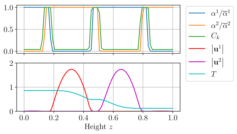
(b)

Figure 11: Probes showing physical quantities, velocity magnitudes and temperatures along the vertical centerline in the (a) baseline design and (b) design optimized with the initial channels and $\Delta P_{\mathit{max}}=5\Delta P_{\mathit{base}}$.

The optimization history of the design with $\Delta P_{\mathit{max}}=5\Delta P_{\mathit{base}}$ and starting with $\xi=0.5$, is seen in Figure 12. Here it is seen that the objective function is very low, near the theoretical maximum, in the early design iterations. The continuation steps are clearly identified, where spikes appear in the constraint function values and where the objective function value rises. The three shown preliminary designs from just prior to the continuation steps clearly illustrate that the two fluids are able to mix, when the projection value is low. This is due to the combination of the identification method discussed in Section 5.3 and the porous formulation.

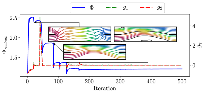
Figure 12: Objective- and constraint function, $\Phi_{\mathit{coolant}}$ and $g_{\gamma}$, respectively, history over design iterations for the optimization with the initial channel design and $\Delta P_{\mathit{max}}=5\Delta P_{\mathit{base}}$. Early design iterations, with low projection sharpness, show that no interface is formed and fluids are not well separated. As the continuation progresses, fluids get more separated, and finally, an interface is formed.

It is hence seen (from the first history state, where the streamlines mix) that the pressure constraint does not really have an influence before the continuation step to $\beta=4$, as the flow is mostly porous prior to this point.

6.2 Three-dimensional shell-and-tube heat exchanger

6.2.1 Problem definition

The second considered case is inspired by a shell-and-tube heat exchanger design. Figure 13 shows the design problem. The heat exchanger has circular in- and outlets of the coolant on one face and circular in- and outlets of the cooled fluid on an adjacent face. Both inlet velocity profiles are assumed to be parabolic with respect to radial distance.

Figure 13: Design domain of the considered heat exchanger. The in- and outlets of the coolant, water, are located on the $y$-min plane (in blue) and the in- and outlets of the cooled fluid, oil, are located on the $x$-max plane (in red). The grey plane is the symmetry plane located at $z=0.5$. The reference length is the height of the heat exchanger, $L=146\cdot 10^{-3}\;\mathrm{[m]}$.

Based on the information, presented in Table 3, the Reynolds- and Peclet numbers of both the cooled and coolant phase can be computed. The solid material is set to be stainless steel, the hot fluid to be oil and the coolant to be water.

Table 3: Parameters of heat exchanger

Property	Cooled side	Coolant side
	Oil, 1	Water, 2
Mass flow $\scriptstyle\dot{m}\;\mathrm{[kg\cdot s^{-1}]}$	$4.57\cdot 10^{-3}$	$9.64\cdot 10^{-4}$
Inlet temperature $\scriptstyle T\;\mathrm{[C]}$	$90$	$65$
Density $\scriptstyle\rho\;\mathrm{[kg\cdot m^{-3}]}$	$866.4$	$980$
Dynamic viscosity $\scriptstyle\mu\;\mathrm{[N\cdot s\cdot m^{2}]}$	$0.0215$	$4.32\cdot 10^{-4}$
Heat capacity $\scriptstyle c_{p}\;\mathrm{[J\cdot kg^{-1}\cdot K^{-1}]}$	$2088$	$4188$
Conductivity $\scriptstyle k\;\mathrm{[W\cdot m^{-1}\cdot K^{-1}]}$	$0.1233$	$0.6$
Solid conductivity $\scriptstyle k\;\mathrm{[W\cdot m^{-1}\cdot K^{-1}]}$	$30$
Pressure drop $\scriptstyle\Delta p\;\mathrm{[Pa]}$	$16402$	$3080$
Reynolds number $\scriptstyle[-]$	$10.9$	$150$
Peclet number $\scriptstyle[-]$	$3973$	$453$

The Reynolds and solid Peclet numbers seen in Table 3 are both converted to their computational equivalents, adjusting for the non-dimensional inlet diameters [23]. The Darcy number is set to $\mathit{Da}=10^{8}$ to limit the porous flow. The final computational parameters are shown in Table 4.

Table 4: Computational parameters of the three dimensional heat exchanger optimization problem.

Property	Cooled	Coolant
Reynolds number $\scriptstyle\mathit{Re}[-]$	$31.32$	$578$
Solid Peclet number $\scriptstyle\mathit{Pe}_{s}[-]$	$46.92$	$34.8$
Conductivity ratio $\scriptstyle C_{k}[-]$	$4.11\cdot 10^{-3}$	$0.02$
Impermeability $\scriptstyle\overline{\alpha}[-]$	$3.19\cdot 10^{6}$	$1.73\cdot 10^{5}$

The optimization is carried out on the half domain, as depicted by the $z=0.5$ plane in Figure 13. The boundary conditions on this plane are of symmetric type, with no-through flux of mass and heat. This symmetric boundary condition constrains the obtained designs to be symmetric. Two baseline designs are considered, both inspired by shell-and-tube heat exchangers. In both cases, the coolant fluid is the tube side. The coolant fluid flows through one or four tubes (respectively half and two tubes in the half domain), in the two baseline designs seen in Figure 14, respectively. Near the plane with the coolant inlet and outlet, a manifold is located which redirects the coolant fluid and a small wall separates the coolant in- and outlet manifolds.

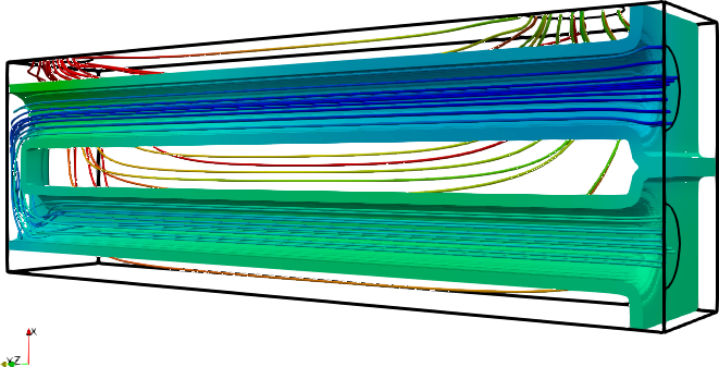
(a) One tube

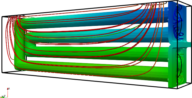
(b) Four tubes

Figure 14: Half baseline designs, with the symmetry plane depicted in Figure 13. Structures and streamlines are colored by temperature, in- and outlets highlighted with black contours, and structure thresholded at $\alpha^{1}>0.1\overline{\alpha}^{1}\land\alpha^{2}>0.1\overline{\alpha}^{2}$.

The baseline designs have different pressure drops and heat transfers, seen in Table 5.

Table 5: Comparison of performance of the two baseline designs.

Design	$\Delta P^{1}_{\mathit{base}}$	$\Delta P^{2}_{\mathit{base}}$	$\Phi_{\mathit{coolant,\,base}}$
1 tube	$11.9$	$3.56$	$4.68$
4 tubes	$57.4$	$3.08$	$7.27$

The baseline designs are optimized with their corresponding pressure drops, i.e. $\Delta P_{\mathit{max}}^{\gamma}=\Delta P_{\mathit{base}}^{\gamma}$. For each baseline pressure drop, four initial designs are considered: One where the design variable is uniform $\xi=0.5$ in the design domain, and three where the respective baseline design is utilized, but subjected to different projection sharpness, $\beta_{\mathit{initial}}=\{1,\;4,\;8\}$. In all cases, the optimization is cut-off after 350 design iterations. The higher initial $\beta$ values ensures more well-defined and impermeable walls. This enables the the coolant flow to travel through the initial tubes, reaching deeper into the domain in the early design iterations. However, for lower $\beta$ values and the uniform distribution of $\xi=0.5$, the walls are either fairly porous or non-existent. This means that the coolant will take the path of least resistance, which is directly from inlet to outlet and not reaching deep into the computational domain. Having the flow fields reaching far into the design domain yields a wider range of spatial sensitivity information. Hence, the flow field in the initial design, and the early design iterations, has a very high impact on the final design and will vary depending on the given problem and boundary conditions.

6.2.2 Results

With both baseline designs, seen in Figure 14, the heat exchanger is optimized using the respective initial baseline designs and $\beta$ values, as previously discussed. All designs are optimized with the maximum pressure drop being equal to the pressure drop in its respective baseline design. In total, eight optimized designs are obtained and the solid structures with streamlines of the designs are seen in Figure 15. For the designs optimized from a loosely-defined initial design ($\beta_{\mathit{initial}}=1$), seen in Figures 15(a)-15(d), the coolant channels do not reach the end of the design domain. However, as seen in Figures 15(e)-15(h), when starting from more well-defined initial designs (higher $\beta_{\mathit{initial}}$), the coolant channels reach further into the design domain,

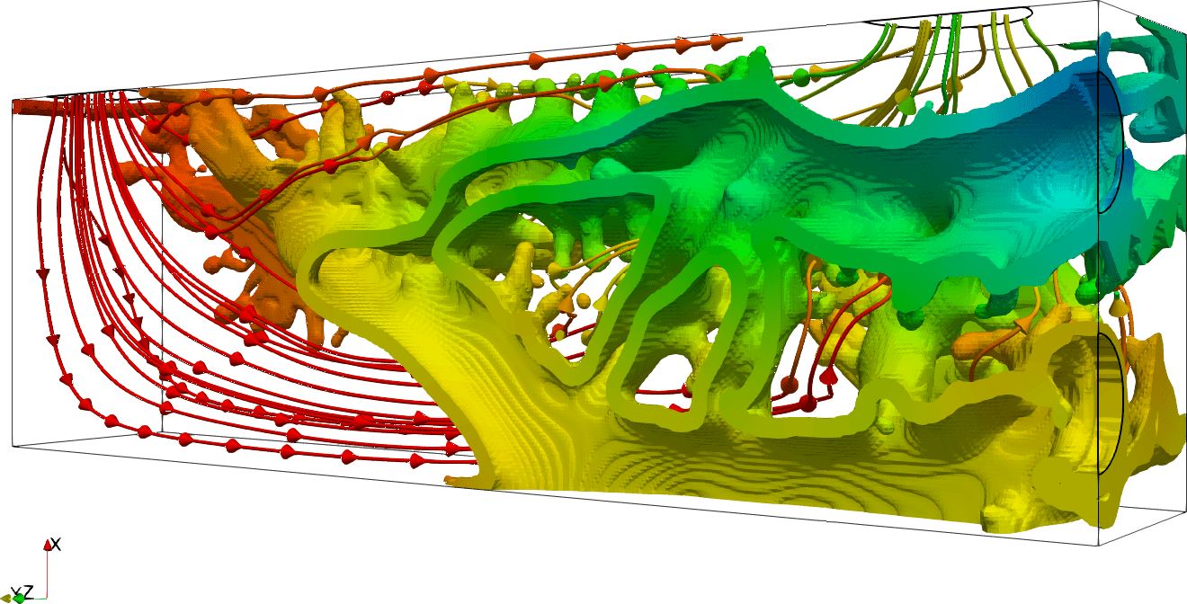
(a) One channel baseline, starting with $\xi=0.5$ and $\beta_{\mathit{initial}}=1$, $\Phi_{\mathit{coolant}}=12.71$

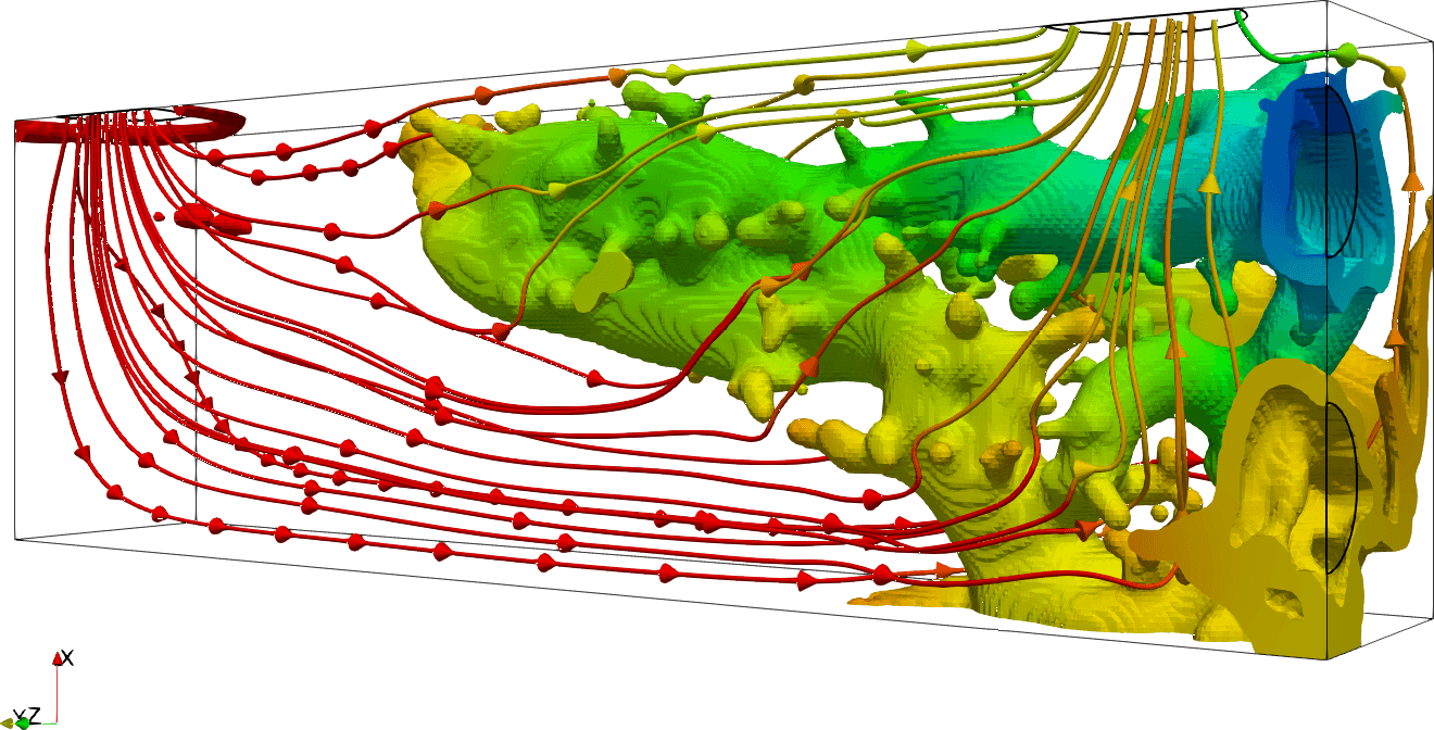
(b) Four channel baseline, starting with $\xi=0.5$ and $\beta_{\mathit{initial}}=1$, $\Phi_{\mathit{coolant}}=13.69$

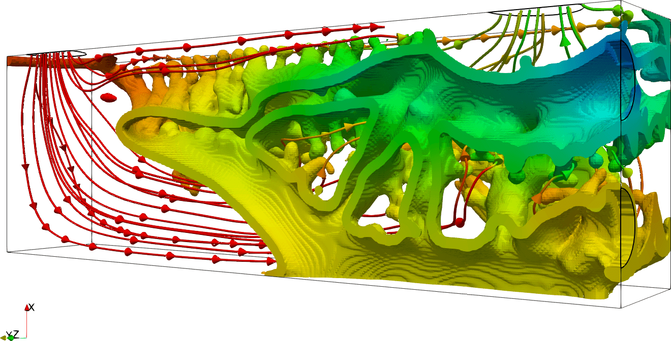
(c) One channel baseline, starting from baseline with $\beta_{\mathit{initial}}=1$, $\Phi_{\mathit{coolant}}=13.31$

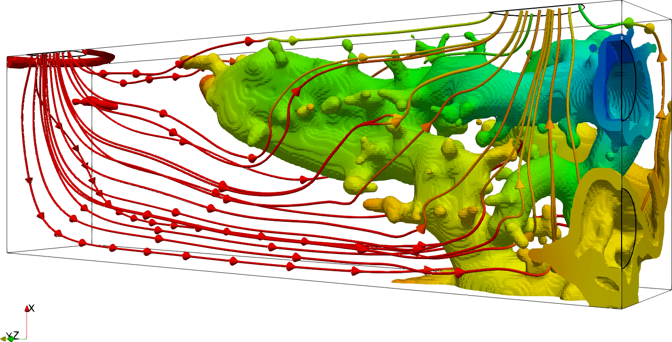
(d) Four channel baseline, starting from baseline with $\beta_{\mathit{initial}}=1$, $\Phi_{\mathit{coolant}}=13.80$

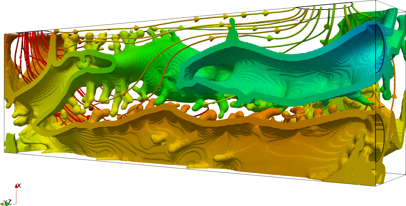
(e) One channel baseline, starting from baseline with $\beta_{\mathit{initial}}=4$, $\Phi_{\mathit{coolant}}=13.44$

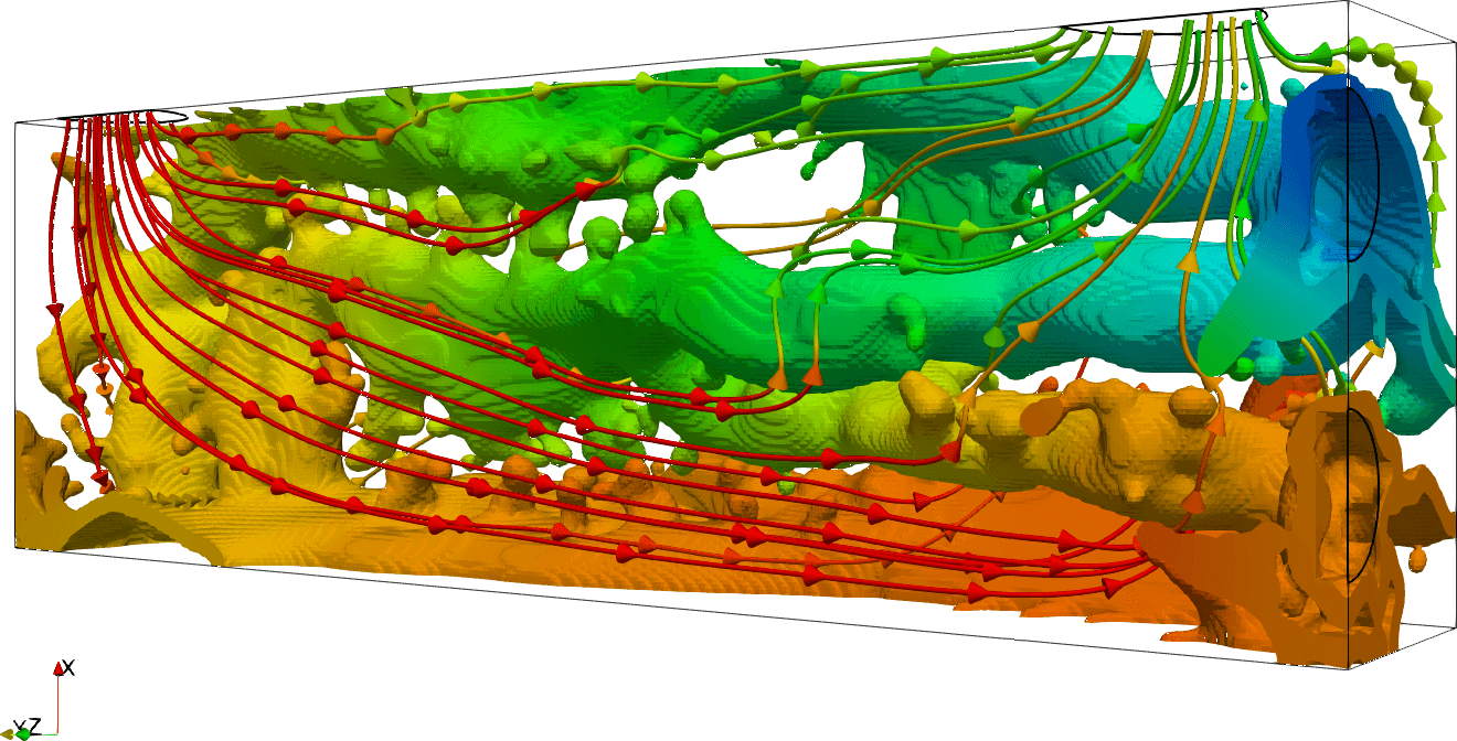
(f) Four channel baseline, starting from baseline with $\beta_{\mathit{initial}}=4$, $\Phi_{\mathit{coolant}}=15.49$

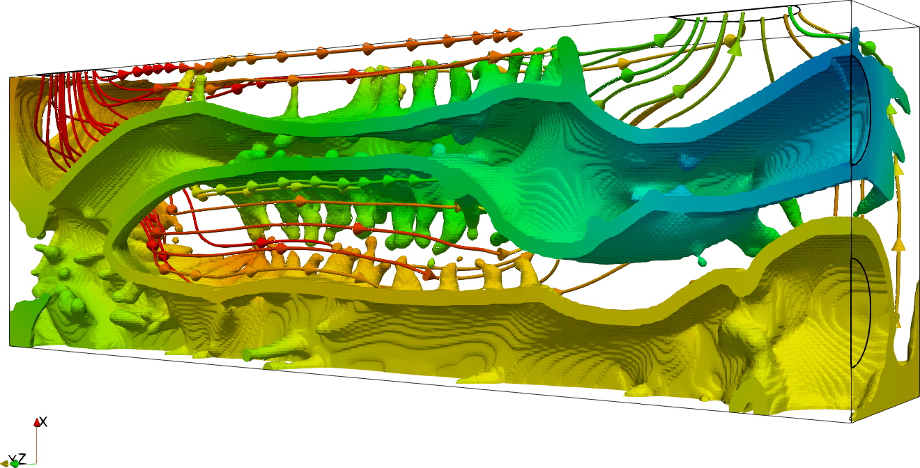
(g) One channel baseline, starting from baseline with $\beta_{\mathit{initial}}=8$, $\Phi_{\mathit{coolant}}=13.34$

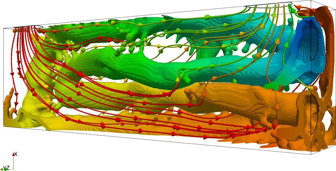
(h) Four channel baseline, starting from baseline with $\beta_{\mathit{initial}}=8$, $\Phi_{\mathit{coolant}}=15.16$

Figure 15: Optimized structures, and corresponding streamlines of the cooled fluid, both colored by temperature. The structures are thresholded at $\alpha^{1}>0.1\overline{\alpha}^{1}\land\alpha^{2}>0.1\overline{\alpha}^{2}$.

On the obtained solid structures, microvilli-like extended features are observed, going into the cooled fluid domain seemingly normal from the coolant tube surface. Microvilli are biological features, which are a part of the cellular membrane, increasing the surface area for absorption and other processes, but holding the volume increase to a minimum. The microvilli-like features from the different tubes are shifted in positions, as seen in the closeup from Figure 16 (from the design seen in Figure 15(f), optimized with $\beta_{\mathit{initial}}=4$ and the four channel baseline initial design field). It is seen that the microvilli-like features are placed in shifted positions relative to each other, such that the flow passes them in a curved manner, which increases the surface area, with flow next to it.

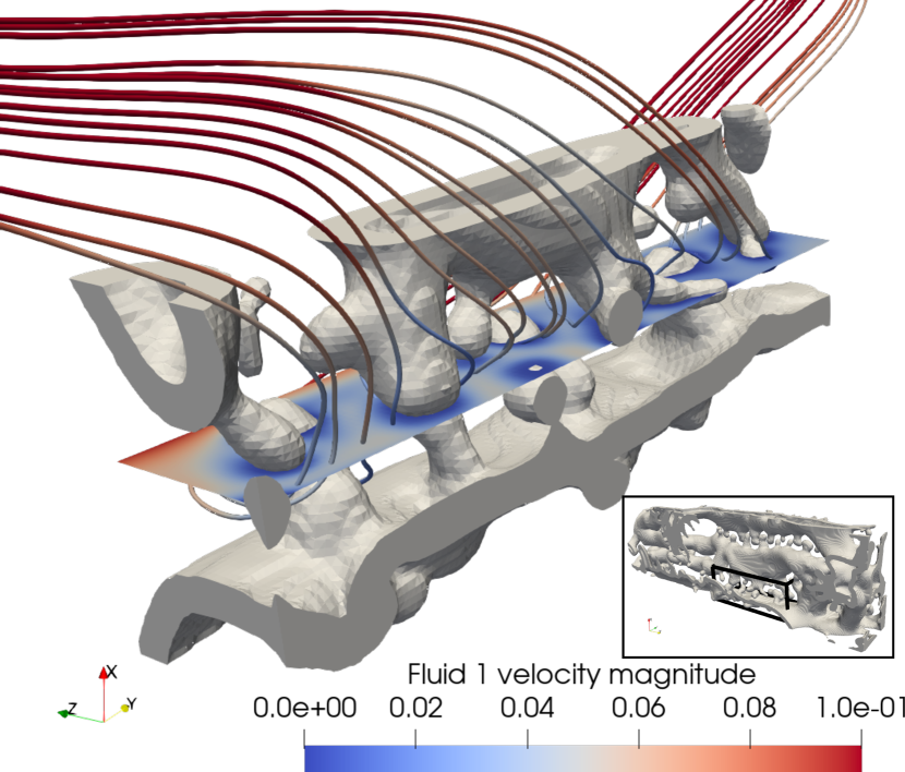
Figure 16: Cut of the solid structure of the design optimized with the four channel baseline, with the initial projection sharpness $\beta_{\mathit{initial}}=4$.The velocity magnitude of the cooled fluid 2 is seen on the plane.

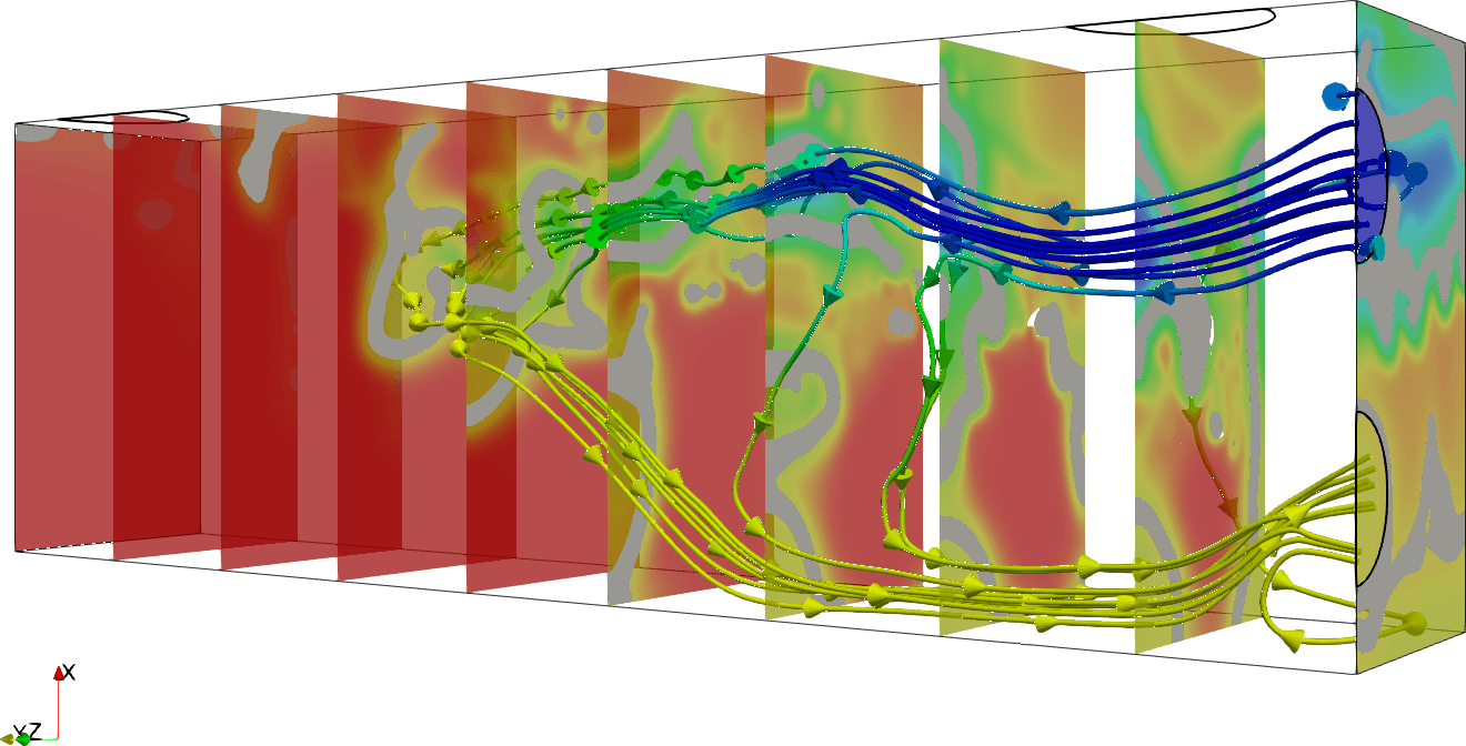
(a) One channel baseline, starting with $\xi=0.5$ and $\beta_{\mathit{initial}}=1$, $\Phi_{\mathit{coolant}}=12.71$

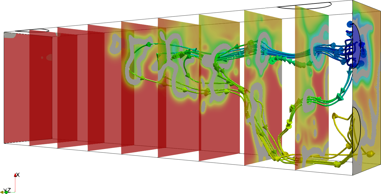
(b) Four channel baseline, starting with $\xi=0.5$ and $\beta_{\mathit{initial}}=1$, $\Phi_{\mathit{coolant}}=13.69$

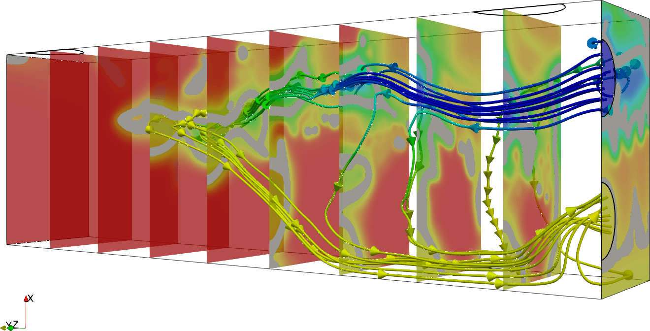
(c) One channel baseline, starting from baseline with $\beta_{\mathit{initial}}=1$, $\Phi_{\mathit{coolant}}=13.31$

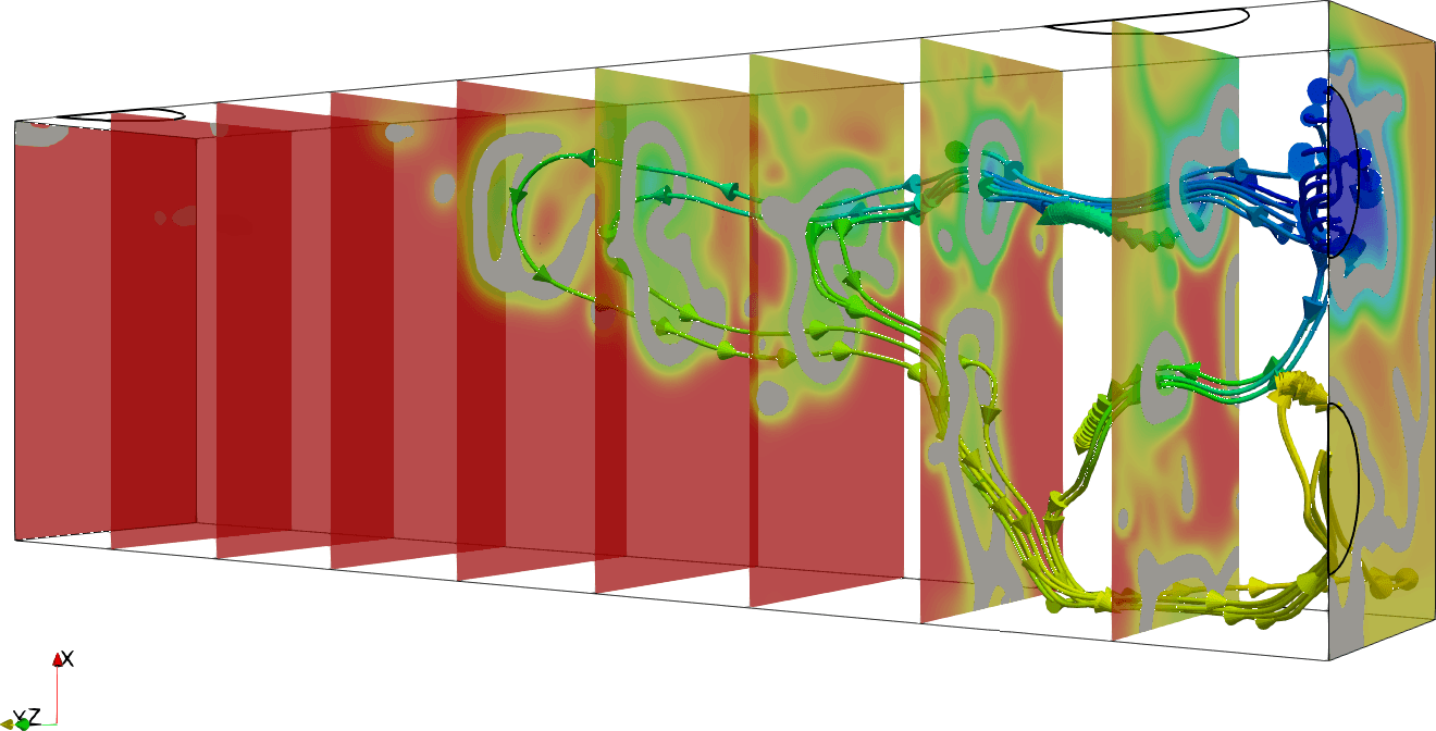
(d) Four channel baseline, starting from baseline with $\beta_{\mathit{initial}}=1$, $\Phi_{\mathit{coolant}}=13.80$

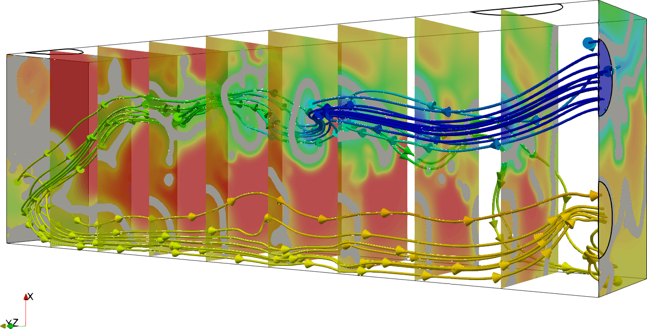
(e) One channel baseline, starting from baseline with $\beta_{\mathit{initial}}=4$$\Phi_{\mathit{coolant}}=13.44$

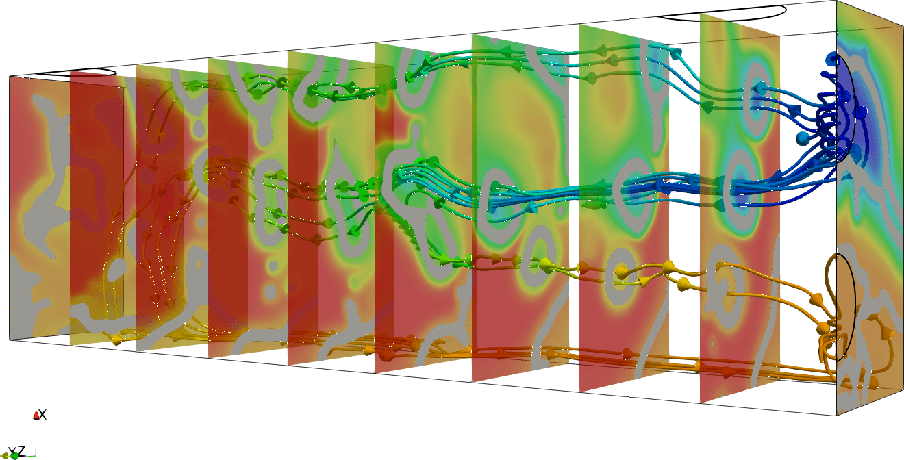
(f) Four channel baseline, starting from baseline with $\beta_{\mathit{initial}}=4$, $\Phi_{\mathit{coolant}}=15.49$

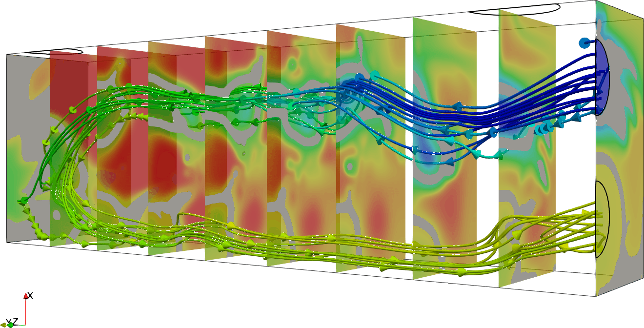
(g) One channel baseline, starting from baseline with $\beta_{\mathit{initial}}=8$, $\Phi_{\mathit{coolant}}=13.34$

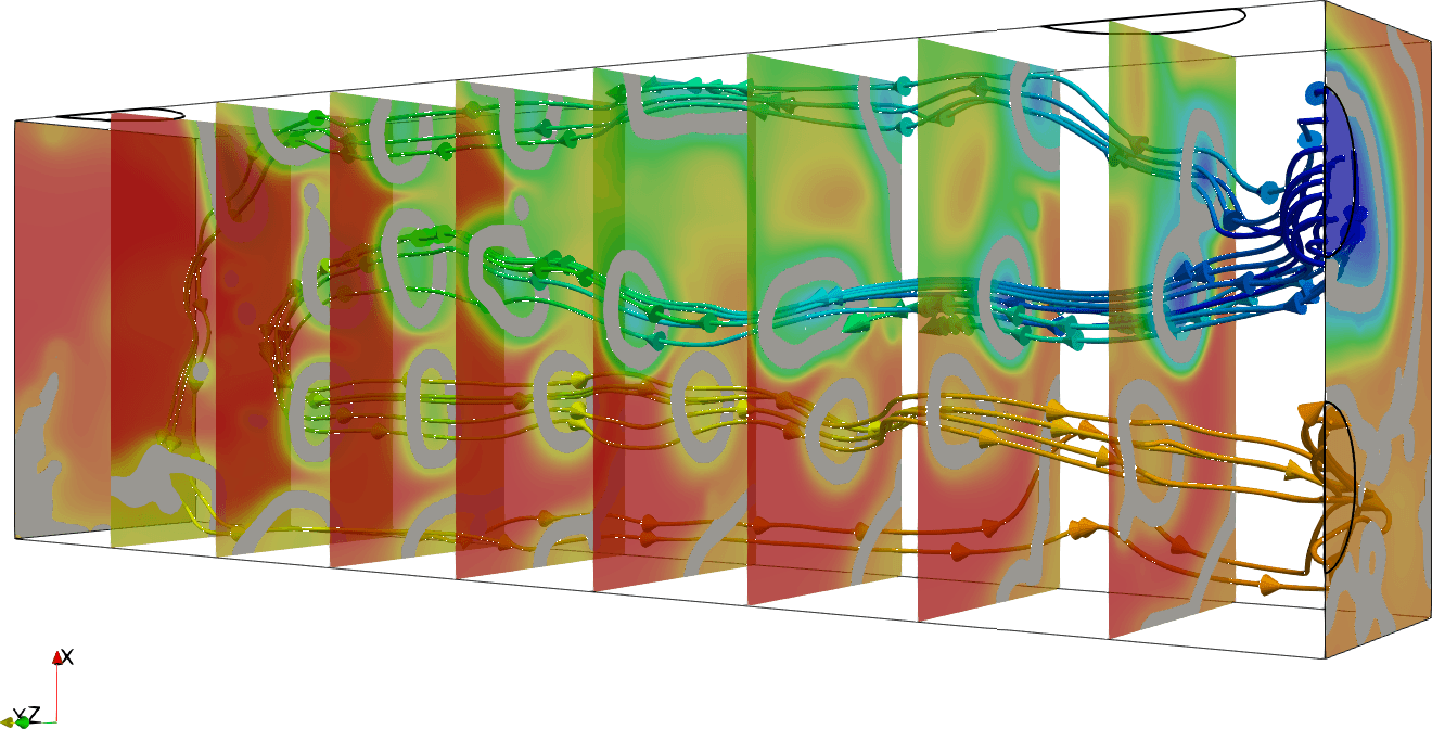
(h) Four channel baseline, starting from baseline with $\beta_{\mathit{initial}}=8$, $\Phi_{\mathit{coolant}}=15.16$

Figure 17: Streamlines of the coolant fluid and slices through the design domain. Slices and streamlines are colored by temperature. The structures (thresholded at $\alpha^{1}>0.1\overline{\alpha}^{1}\land\alpha^{2}>0.1\overline{\alpha}^{2}$) on the slices are colored in grey.

Figure 17 shows the flow of the tube side coolant. It is again observed that starting with an initial design, where the coolant flow reaches the back of the domain, results in designs, where the coolant channels are present in the entirety of the domain. However, for the designs where the coolant flow did not reach far into the computational domain, Figures 17(a)-17(d), it is seen that the back of the domain is almost unused, as neither structures nor visible temperature variations are present in these areas. The entirety of the design domain is hence not fully exploited when starting with a too poorly-defined and permeable initial design. On the other hand, when a higher initial projection sharpness is used, the topology of the initial design of the coolant fluid is preserved to a certain extent, as shown in Figures 17(e)-17(h). The designs obtained with $\beta_{\mathit{initial}}>1$ and the one channel baseline design, seen in Figures 15(e), 15(g), 17(e) and 17(g), have a topology similar to the one seen in the baseline, Figure 14(a). The coolant channels are, for the most part, attached to the symmetry plane. The upper channel of the design optimized with $\beta_{\mathit{initial}}=4$ is detached from the symmetry plane for a little distance. This increases the contact surface between the fluids and the solid, but probably also has an influence on the heat transfer coefficient.

When using the baseline design with four channels, Figure 14(b), and $\beta_{\mathit{initial}}>1$, the optimized designs seen in Figures 15(f), 15(h), 17(f) and 17(h), have coolant fluid domain topologies, that also are preserved to a certain extent. The coolant fluid channel paths are, however, modified significantly in comparison to the baseline design. This also affects the flow of the cooled fluid, which the optimized structure disturbs more than what is observed in the baseline design. This higher disturbance of the cooled flow probably also is of benefit to the heat transfer.

Table 6 shows the obtained heat transfer in the different optimized designs. All optimized designs perform better, than both baselines, whose heat transfers also are seen in Table 6. The relative improvements, compared to the better 4 channel baseline, range from $74.8\%$ (starting from $\beta_{\mathit{initial}}=1$, $\xi=0.5$ and using one channel design pressure drops) to $113\%$ (starting from $\beta_{\mathit{initial}}=4$ with the four channel baseline). Furthermore, with both baseline designs, it is seen that the designs optimized with the initial projection sharpness $\beta_{\mathit{initial}}=4$ are the ones performing best.

Table 6: Comparison of the thermal energy flux out of the cold fluid. It is seen that there, in all cases, is a considerable improvement of the baseline design. The designs optimized with the 4 channels baseline design always perform better. Furthermore, with both baseline designs, starting with $\beta=4$ yields the best design.

		1 channel	4 channels
Baseline design		$4.68$	$7.27$
Optimized	$\xi_{\mathit{initial}}=0.5$, $\beta_{\mathit{initial}}=1$	$12.71$	$13.69$
	$\beta_{\mathit{initial}}=1$	$13.31$	$13.80$
	$\beta_{\mathit{initial}}=4$	$13.44$	$15.49$
	$\beta_{\mathit{initial}}=8$	$13.34$	$15.16$

Redimensionalizing the best optimized design, the transferred thermal power is obtained, to be $P=89.9\;\mathrm{W}$. Likewise, the best baseline (4 channels), has a transferred thermal power of $P=42.2\;\mathrm{W}$.

7 Discussion and conclusion

In this paper, a new approach for topology optimization of two fluid heat exchangers is presented. The formulation, based on a single design variable field, guarantees the presence of a solid interface between the two fluid phases based on an erosion-dilation identification method. The two mass transfer and one heat transfer problems are solved sequentially in the entirety of the design domain. The optimization maximizes the amount of transferred heat with maximum pressure drop constraints on both fluids. The methodology is applied to two numerical examples.

In the two-dimensional counter-flow example where the design freedom is limited, it is seen that the channels are made narrower, as the allowable pressure drop is increased. This provides an excellent agreement between the amount of transferred heat and the maximum allowable pressure drop obtained using Poiseuille flow and the $\epsilon-\mathit{NTU}$ method. This indicates that the improvement in heat transfer, obtained with the topology optimization process introduced here, can be related to a theoretically derived optimum (for a ”one-dimensional” optimization) - at least for this simple case.

In the three-dimensional example, simple shell-and-tube-like baseline designs were significantly enhanced, with up to a $113\%$ improvement compared to the best-performing baseline. In the obtained results, the importance of the flow field in the initial design was highlighted. This relates to the computation of the sensitivities in the early design iterations, which are crucial to the later optimization process. In the optimized designs, microvilli-like features are observed, which enhance both the surface area, but also perturb the flow near them.

The novel and intricate designs appearing when utilizing the presented methodology have been challenging to export to a CAD-based engineering analysis environment. More research into the transformation from density-based representations to CAD/spline basis are needed. In order to evaluate the performance of the obtained designs, a post-evaluation in a commercial software using a segregated approach would indeed be relevant. However, we have so far not been successful in developing a methodology able to transfer the complex optimized designs for further processing. Thus, the obtained designs may at present remain inspirational for future heat exchanger designs.

In this first work on systematic heat-exchanger design with well-defined wall-thickness using topology optimization, we have focused on method development and providing examples with ultimate design freedom, which amongst others resulted in the interesting appearance of microvillies. Such intricate geometrical details will probably not be relevant for practical systems, but give valuable insight. As discussed above, such details may also be difficult to handle geometrically - also manufacturing-wise, even with advance additive manufacturing techniques. To hinder such complexity and ensure manufacturability, we may in future work include more restrictive geometry constraints like larger length-scale, overhang or extrusion constraints, keeping in mind that every constraint imposed will decrease the achievable heat exchanger efficiencies.

Appendix A Weak formulations and stabilization parameters

A.1 Mass transfer

The weak form of the Navier-Stokes equations (1,2) is to be found in the follwing. For this purpose, the finite dimensional trial- and test function spaces for the velocity, $\mathcal{S}_{u}$ and $\mathcal{V}_{u}$, and for the pressure, $\mathcal{S}_{p}$ and $\mathcal{V}_{p}$, respectively, are introduced. The trial functions $u_{i}\in\mathcal{S}_{u}$ and $p\in\mathcal{S}_{p}$ shall be found such that the test functions $\forall w_{i}\in\mathcal{V}_{u}$ and $\forall q\in\mathcal{V}_{p}$. After multiplication by the test functions, the expressions are integrated over the volume $\Omega$.

After integration by parts with the assumption of no outward surface traction, the weak form yields:

$$\begin{split}\mathscr{R}^{u}&=\int_{\Omega}w_{i}u_{i}\frac{\partial u_{j}}{\partial x_{i}}dV+\int_{\Omega}\frac{1}{Re}\frac{\partial w_{i}}{\partial x_{j}}\left(\frac{\partial u_{i}}{\partial x_{j}}+\frac{\partial u_{j}}{\partial x_{i}}\right)dV\\ &\qquad-\int_{\Omega}\frac{\partial w_{i}}{\partial x_{i}}PdV+\int_{\Omega}w_{i}\alpha u_{i}dV=0\\ \mathscr{R}^{p}&=\int_{\Omega}q\frac{\partial u_{i}}{\partial x_{i}}dV=0\end{split}$$ (35)

As discussed in Section 4, the residual functionals are stabilised, by adding both SUPG and PSPG stabilisations, $\mathscr{F}^{\delta}$ and $\mathscr{F}^{\epsilon}$, respectively:

$$\begin{split}\tilde{\mathscr{R}^{u}}&=\mathscr{R}^{u}+\mathscr{F}^{\delta}=0\\ \tilde{\mathscr{R}^{p}}&=\mathscr{R}^{p}+\mathscr{F}^{\epsilon}=0\end{split}$$ (36)

The weak SUPG- and PSPG stabilisation terms are given as a function of $R^{u}_{i}$, the residual from the strong form Navier-Stokes formulation [48]:

$$\mathscr{F}^{\delta} =\sum_{e=1}^{N_{e}}\int_{\Omega_{e}}\tau_{SU}u_{i}\frac{\partial w_{j}}{\partial x_{i}}R_{j}^{u}dV$$ (37)

$$\mathscr{F}^{\epsilon} =\sum_{e=1}^{N_{e}}\int_{\Omega_{e}}\tau_{PS}\frac{\partial q}{\partial x_{j}}R_{j}^{u}dV$$ (38)

The stabilization factors, $\tau_{\mathit{SU}}$ and $\tau_{\mathit{PS}}$, used for the mass transfer problems SUPG and PSPG stabilization, respectively, are the same. It is almost identical to the one used by [23]:

$$\tau_{\mathit{SU}}=\tau_{\mathit{PS}}=\tau=\left(\frac{1}{\tau_{1}^{r}}+\frac{1}{\tau_{3}^{r}}+\alpha^{r}\right)^{-\frac{1}{r}}$$ (39)

where the power in the minimum function is set to $r=2$. The factors are given as:

$$\tau_{1} =\frac{4h_{e}}{\left|\left|\mathbf{u}_{e}\right|\right|_{2}}$$ (40)

$$\tau_{3} =\frac{h_{e}^{2}\mathit{Re}}{4}$$ (41)

The derivatives of the stabilization parameter with respect the velocity state and to the design variable, used for the computation of the Jacobian matrix and of the sensitivities, are given as:

$$\frac{\partial\tau}{\partial\mathbf{u}_{e}} =\frac{1}{\tau_{1}^{3}}\left(\frac{1}{\tau_{1}^{2}}+\frac{1}{\tau_{3}^{2}}+\alpha^{2}\right)^{-\frac{3}{2}}\left(-\tau_{1}\left(\mathbf{u}_{e}^{\intercal}\mathbf{u}_{e}\right)^{-1}\mathbf{u}_{e}^{\intercal}\right)$$ (42)

$$\frac{\partial\tau}{\partial\xi} =-\alpha\left(\frac{1}{\tau_{1}^{2}}+\frac{1}{\tau_{3}^{2}}+\alpha^{2}\right)^{-\frac{3}{2}}\frac{\partial\alpha}{\partial\xi}$$ (43)

A.2 Heat transfer

The weak form of the heat transfer problem from (6) is obtained by introducing the trial- and test function spaces, $\mathcal{S}_{T}$ and $\mathcal{V}_{T}$, respectively. The finite element problem hence translates to finding a temperature field (trial function) $T\in\mathcal{S}_{T}$, such that the test function $\forall v\in\mathcal{V}_{T}$. After integration by part, and assuming no outward surface heat flux (i.e. the domain is insulated), the variational formulation yields.

$$\mathscr{R}^{T}=\int_{\Omega}v\sum_{\gamma=1}^{\mathit{NF}}\left(\mathit{Pe}_{s}^{\gamma}u_{i}^{\gamma}\right)\frac{\partial T}{\partial x_{i}}dV+\int_{\Omega}C_{k}\frac{\partial v}{\partial x_{i}}\frac{\partial T}{\partial x_{i}}dV=0$$ (44)

The residual is stabilised with a SUPG stabilisation scheme, $\mathscr{F}^{\zeta}$:

$$\tilde{\mathscr{R}^{T}}=\mathscr{R}^{T}+\mathscr{F}^{\zeta}=0$$ (45)

As in the mass transfer, the weak stabilization term is given as a function of the strong for residual $R_{i}^{T}$, obtained from (6), as well as the convection term, $\sum_{\gamma=1}^{\mathit{NF}}\left(\mathit{Pe}_{s}^{\gamma}u_{i}^{\gamma}\right)$:

$$\mathscr{F}^{\zeta}=\sum_{e}^{N_{e}}\int_{\Omega_{e}}\tau_{SU_{T}}\sum_{\gamma=1}^{\mathit{NF}}\left(\mathit{Pe}_{s}^{\gamma}u_{i}^{\gamma}\right)\frac{\partial v}{\partial x_{i}}R^{T}_{i}dV$$ (46)

The factor for the SUPG stabilization of the heat transfer, $\tau_{\mathit{SU}_{T}}$, is given as used by [23]:

$$\tau_{\mathit{SU}_{T}}=\left(\frac{1}{\tau_{\mathit{1,T}}^{r}}+\frac{1}{\tau_{\mathit{3,T}}^{r}}\right)^{-\frac{1}{r}}$$ (47)

where the power in the min function is set to $r=2$. The factors are given as:

$$\tau_{\mathit{1,T}} =\frac{4h_{e}}{\left|\left|\left(\mathbf{u}_{e}^{1}\mathit{Pe}^{1}+\mathbf{u}_{e}^{2}\mathit{Pe}^{2}\right)\right|\right|_{2}}$$ (48)

$$\tau_{\mathit{3,T}} =\frac{h_{e}^{2}}{4C_{k}}$$ (49)

The velocity and design variable derivatives of the stabilization parameters are:

$$\frac{\partial\tau_{\mathit{SU}_{T}}}{\partial\mathbf{u}_{e}^{\gamma}} =-\tau_{\mathit{SU}_{T}}^{3}\frac{\mathit{Pe}^{\gamma}}{16h_{e}^{2}}\left(\mathbf{u}_{e}^{1}\mathit{Pe}^{1}+\mathbf{u}_{e}^{2}\mathit{Pe}^{2}\right)$$ (50)

$$\frac{\partial\tau_{\mathit{SU}_{T}}}{\partial\xi} =\frac{1}{\tau_{\mathit{3,T}}^{3}}\left(\frac{1}{\tau_{\mathit{1,T}}^{2}}+\frac{1}{\tau_{\mathit{3,T}}^{2}}\right)^{-\frac{3}{2}}\left(-\frac{h_{e}^{2}}{4C_{k}^{2}}\right)\frac{\partial C_{k}}{\partial\xi}$$ (51)

Appendix B Notes on sensitivity analysis

B.1 Adjoint sensitivity analysis

In order to find the sensitivities of a function, the Lagrangian function, with the arbitrary Lagrangian multipliers, as seen in Equation (24), is set up. Differentiating this function with respect to the design variable, and invoking the chain rule on all terms gives:

$$\begin{split}\frac{\mathrm{d}\mathcal{L}}{\mathrm{d}\xi}=\frac{\partial\Phi}{\partial\xi}+&\sum_{s=\{\mathit{F1},\;\mathit{F2},\;\mathit{T}\}}\left(\frac{\partial\Phi}{\partial\mathbf{s}}\frac{\mathrm{d}\mathbf{s}}{\mathrm{d}\xi}+\right.\\ &\bm{\lambda}_{s}^{\intercal}\frac{\partial\mathbf{R}_{s}}{\partial\xi}+\bm{\lambda}_{s}^{\intercal}\frac{\partial\mathbf{R}_{s}}{\partial\mathbf{u_{1}}}\frac{\mathrm{d}\mathbf{u_{1}}}{\mathrm{d}\xi}+\\ &\left.\bm{\lambda}_{s}^{\intercal}\frac{\partial\mathbf{R}_{s}}{\partial\mathbf{u_{2}}}\frac{\mathrm{d}\mathbf{u_{2}}}{\mathrm{d}\xi}+\bm{\lambda}_{s}^{\intercal}\frac{\partial\mathbf{R}_{s}}{\partial T}\frac{\mathrm{d}T}{\mathrm{d}\xi}\right)\end{split}$$ (52)

where the summation over $s$ signifies, that the operation is repeated for both mass transfer- and the heat transfer state. As the two mass transfer states are mutually independent, and the coupling between the two mass transfers is weak, the corresponding terms in (52) can be left out. The Lagrangian multipliers, being arbitrary allows to set certain terms to zero:

$$\begin{split}\frac{\mathrm{d}\mathcal{L}}{\mathrm{d}\xi}=\frac{\partial\Phi}{\partial\xi}+&\bm{\lambda}_{F1}^{\intercal}\frac{\partial\mathbf{R}_{F1}}{\partial\xi}+\bm{\lambda}_{F2}^{\intercal}\frac{\partial\mathbf{R}_{F2}}{\partial\xi}+\bm{\lambda}_{T}^{\intercal}\frac{\partial\mathbf{R}_{T}}{\partial\xi}\\ +&\underbrace{\left(\frac{\partial\Phi}{\partial\mathbf{u_{1}}}+\bm{\lambda}_{F1}^{\intercal}\frac{\partial\mathbf{R}_{F1}}{\partial\mathbf{u_{1}}}+\bm{\lambda}_{T}^{\intercal}\frac{\partial\mathbf{R}_{T}}{\partial\mathbf{u_{1}}}\right)}_{=0}\frac{\mathrm{d}\mathbf{u_{1}}}{\mathrm{d}\xi}\\ +&\underbrace{\left(\frac{\partial\Phi}{\partial\mathbf{u_{2}}}+\bm{\lambda}_{F2}^{\intercal}\frac{\partial\mathbf{R}_{F2}}{\partial\mathbf{u_{2}}}+\bm{\lambda}_{T}^{\intercal}\frac{\partial\mathbf{R}_{T}}{\partial\mathbf{u_{2}}}\right)}_{=0}\frac{\mathrm{d}\mathbf{u_{2}}}{\mathrm{d}\xi}\\ +&\underbrace{\left(\frac{\partial\Phi}{\partial T}+\bm{\lambda}_{T}^{\intercal}\frac{\partial\mathbf{R}_{T}}{\partial T}\right)}_{=0}\frac{\mathrm{d}T}{\mathrm{d}\xi}\end{split}$$ (53)

which hence allows for the elimination of the difficult terms $\frac{\mathrm{d}\mathbf{u_{1}}}{\mathrm{d}\xi}$, $\frac{\mathrm{d}\mathbf{u_{2}}}{\mathrm{d}\xi}$ and $\frac{\mathrm{d}T}{\mathrm{d}\xi}$, by solving the adjoint problems, outlined in Equations (26-28). The sensitivities are then found using the Lagrangian multipliers computed by solving the adjoint problems, as seen in Equation (25).

B.2 Chain rule projection of sensitivities

The sensitivities of the objective function, and of the constraints, are found with respect to $\xi_{1}$ and $\xi_{2}$ , as described in Section 5.5 and B.1. These sensitivities $\frac{\partial\Phi}{\partial\xi_{1}}$ and $\frac{\partial\Phi}{\partial\xi_{2}}$, are projected back to $\frac{\partial\Phi}{\partial\xi}$ using the chain rule:

$$\frac{\partial\Phi}{\partial\xi}=\frac{\partial\Phi}{\partial\xi}+\frac{\mathrm{d}\Phi}{\mathrm{d}\xi_{1}}\frac{\partial\xi_{1}}{\partial\xi}+\frac{\mathrm{d}\Phi}{\mathrm{d}\xi_{2}}\frac{\partial\xi_{2}}{\partial\xi}$$ (54)

The sensitivities with respect to the eroded and dilated variables are projected back to the design variable $\xi$ with steps corresponding to the one of the erosion dilation process from Section 5.3. Keeping in mind that $\frac{\partial\xi_{1}}{\partial\hat{\tilde{\xi}}_{1}}=-1$, the chain-rule terms are given as:

$$\frac{\partial\xi_{1}}{\partial\xi} =-\frac{\partial\hat{\tilde{\xi}}_{1}}{\partial\hat{\tilde{\xi}}}\frac{\partial\hat{\tilde{\xi}}}{\partial\hat{\xi}}\frac{\partial\hat{\xi}}{\partial\tilde{\xi}}\frac{\partial\tilde{\xi}}{\partial\xi}$$ (55)

$$\frac{\partial\xi_{2}}{\partial\xi} =\frac{\partial\hat{\tilde{\xi}}_{2}}{\partial\hat{\tilde{\xi}}}\frac{\partial\hat{\tilde{\xi}}}{\partial\hat{\xi}}\frac{\partial\hat{\xi}}{\partial\tilde{\xi}}\frac{\partial\tilde{\xi}}{\partial\xi}$$ (56)

The chain rule terms $\frac{\partial\hat{\tilde{\xi}}_{\gamma}}{\partial\xi}$ and $\frac{\partial\hat{\xi}}{\partial\xi}$ are found by differentiation of the smooth Heaviside projection from Equation (18):

$$\frac{\partial\hat{\xi}}{\partial\tilde{\xi}}=\beta\frac{1-\tanh^{2}(\beta(\tilde{\xi}-\eta))}{\tanh(\beta\eta)+\tanh(\beta(1-\eta))}$$ (57)

The filtering operation terms from the chain rule, $\frac{\partial\hat{\tilde{\xi}}}{\partial\hat{\xi}}$ and $\frac{\partial\tilde{\xi}}{\partial\xi}$, are equivalent to filtering the sensitivities through the PDE filter, as was done with $\xi$ to obtain $\tilde{\xi}$ and with $\hat{\xi}$ to obtain $\hat{\tilde{\xi}}$ [42].

References

- Incropera [2013] F. P. Incropera, Foundations of heat transfer, 6., international student version ed., John Wiley, Singapore, 2013.
- Awais and Bhuiyan [2018] M. Awais, A. A. Bhuiyan, Heat and mass transfer for compact heat exchanger (chxs) design: A state-of-the-art review, International Journal of Heat and Mass Transfer 127 (2018) 359 – 380. doi:https://doi.org/10.1016/j.ijheatmasstransfer.2018.08.026.
- Bhutta et al. [2012] M. M. A. Bhutta, N. Hayat, M. H. Bashir, A. R. Khan, K. N. Ahmad, S. Khan, Cfd applications in various heat exchangers design: A review, Applied Thermal Engineering 32 (2012) 1 – 12. doi:https://doi.org/10.1016/j.applthermaleng.2011.09.001.
- Conflux [2020] Conflux, Conflux technology website, https://www.confluxtechnology.com/, 2020. Accessed: 02-05-2020.
- nTopology [2019] nTopology, Taking Heat Exchanger Design to the Next Level with High-Performance Geometry - nTopology blog entry, https://ntopology.com/blog/2019/12/16/taking-heat-exchanger-design-to-the-next-level-with-high-performance-geometry/, 2019. Accessed: 02-05-2020.
- Bendsøe and Kikuchi [1988] M. P. Bendsøe, N. Kikuchi, Generating optimal topologies in structural design using a homogenization method, Computer Methods in Applied Mechanics and Engineering 71 (1988) 197–224. doi:10.1016/0045-7825(88)90086-2.
- Sigmund and Maute [2013] O. Sigmund, K. Maute, Topology optimization approaches: A comparative review, Structural and Multidisciplinary Optimization 48 (2013) 1031–1055. doi:10.1007/s00158-013-0978-6.
- Alexandersen and Andreasen [2020] J. Alexandersen, C. S. Andreasen, A review of topology optimisation for fluid-based problems, Fluids 5 (2020) 1–32. doi:10.3390/fluids5010029.
- Borrvall and Petersson [2003] T. Borrvall, J. Petersson, Topology optimization of fluids in stokes flow, International Journal for Numerical Methods in Fluids 41 (2003) 77–107. doi:10.1002/fld.426.
- Aage et al. [2008] N. Aage, T. H. Poulsen, A. Gersborg-Hansen, O. Sigmund, Topology optimization of large scale stokes flow problems, Structural and Multidisciplinary Optimization 35 (2008) 175–180. doi:10.1007/s00158-007-0128-0.
- Challis and Guest [2009] V. J. Challis, J. K. Guest, Level set topology optimization of fluids in stokes flow, International Journal for Numerical Methods in Engineering 79 (2009) 1284–1308. doi:10.1002/nme.2616.
- Evgrafov [2014] A. Evgrafov, State space newton’s method for topology optimization, Computer Methods in Applied Mechanics and Engineering 278 (2014) 272–290. doi:10.1016/j.cma.2014.06.005.
- Yonekura and Kanno [2017] K. Yonekura, Y. Kanno, Topology optimization method for interior flow based on transient information of the lattice boltzmann method with a level-set function, Japan Journal of Industrial and Applied Mathematics 34 (2017) 611–632. doi:10.1007/s13160-017-0257-9.
- Villanueva and Maute [2017] C. H. Villanueva, K. Maute, Cutfem topology optimization of 3d laminar incompressible flow problems, Computer Methods in Applied Mechanics and Engineering 320 (2017) 444–473. doi:10.1016/j.cma.2017.03.007.
- Chen et al. [2017] C. Chen, K. Yaji, T. Yamada, K. Izui, S. Nishiwaki, Local-in-time adjoint-based topology optimization of unsteady fluid flows using the lattice boltzmann method, Mechanical Engineering Journal 4 (2017) 17–00120–17–00120. doi:10.1299/mej.17-00120.
- Dilgen et al. [2018] C. B. Dilgen, S. B. Dilgen, D. R. Fuhrman, O. Sigmund, B. S. Lazarov, Topology optimization of turbulent flows, Computer Methods in Applied Mechanics and Engineering 331 (2018) 363–393. doi:10.1016/j.cma.2017.11.029.
- Łaniewski Wołłk and Rokicki [2016] L. Łaniewski Wołłk, J. Rokicki, Adjoint lattice boltzmann for topology optimization on multi-gpu architecture, Computers & Mathematics with Applications 71 (2016) 833–848. doi:10.1016/j.camwa.2015.12.043.
- Haertel and Nellis [2017] J. H. Haertel, G. F. Nellis, A fully developed flow thermofluid model for topology optimization of 3d-printed air-cooled heat exchangers, Applied Thermal Engineering 119 (2017) 10–24. doi:10.1016/j.applthermaleng.2017.03.030.
- Haertel et al. [2018] J. H. Haertel, K. Engelbrecht, B. S. Lazarov, O. Sigmund, Topology optimization of a pseudo 3d thermofluid heat sink model, International Journal of Heat and Mass Transfer 121 (2018) 1073–1088. doi:10.1016/j.ijheatmasstransfer.2018.01.078.
- Yaji et al. [2018] K. Yaji, M. Ogino, C. Chen, K. Fujita, Large-scale topology optimization incorporating local-in-time adjoint-based method for unsteady thermal-fluid problem, Structural and Multidisciplinary Optimization 58 (2018) 817–822. doi:10.1007/s00158-018-1922-6.
- Dilgen et al. [2018] S. B. Dilgen, C. B. Dilgen, D. R. Fuhrman, O. Sigmund, B. S. Lazarov, Density based topology optimization of turbulent flow heat transfer systems, Structural and Multidisciplinary Optimization 57 (2018) 1905–1918. doi:10.1007/s00158-018-1967-6.
- Pietropaoli et al. [2019] M. Pietropaoli, F. Montomoli, A. Gaymann, Three-dimensional fluid topology optimization for heat transfer, Structural and Multidisciplinary Optimization 59 (2019) 801–812. doi:10.1007/s00158-018-2102-4.
- Alexandersen et al. [2016] J. Alexandersen, O. Sigmund, N. Aage, Large scale three-dimensional topology optimisation of heat sinks cooled by natural convection, International Journal of Heat and Mass Transfer 100 (2016) 876–891. doi:10.1016/j.ijheatmasstransfer.2016.05.013.
- Alexandersen et al. [2018] J. Alexandersen, O. Sigmund, K. E. Meyer, B. S. Lazarov, Design of passive coolers for light-emitting diode lamps using topology optimisation, International Journal of Heat and Mass Transfer 122 (2018) 138–149. doi:10.1016/j.ijheatmasstransfer.2018.01.103.
- Pollini et al. [2020] N. Pollini, O. Sigmund, C. S. Andreasen, J. Alexandersen, A “poor man’s” approach for high-resolution three-dimensional topology design for natural convection problems, Advances in Engineering Software 140 (2020) 102736. doi:https://doi.org/10.1016/j.advengsoft.2019.102736.
- Sun et al. [2018] C. Sun, N. Lewpiriyawong, K. L. Khoo, S. Zeng, P. S. Lee, Thermal enhancement of fin and tube heat exchanger with guiding channels and topology optimisation, International Journal of Heat and Mass Transfer 127 (2018) 1001–1013. doi:10.1016/j.ijheatmasstransfer.2018.08.093.
- Kobayashi et al. [2019] H. Kobayashi, K. Yaji, S. Yamasaki, K. Fujita, Freeform winglet design of fin-and-tube heat exchangers guided by topology optimization, Applied Thermal Engineering 161 (2019). doi:10.1016/j.applthermaleng.2019.114020.
- Papazoglou [2015] P. Papazoglou, Topology Optimization of Heat Exchangers, Master’s thesis, Delft University of Technology, 2015. URL: http://resolver.tudelft.nl/uuid:08481ec6-d6df-4162-b254-8b99eeccc6d1.
- Haertel [2018] J. Haertel, Design of Thermal Systems Using Topology Optimization, Ph.D. thesis, Technical University of Denmark, 2018. URL: https://orbit.dtu.dk/en/publications/design-of-thermal-systems-using-topology-optimization.
- Tawk et al. [2019] R. Tawk, B. Ghannam, M. Nemer, Topology optimization of heat and mass transfer problems in two fluids—one solid domains, Numerical Heat Transfer, Part B: Fundamentals 76 (2019) 1–22. doi:10.1080/10407790.2019.1644919.
- Saviers et al. [2019] K. R. Saviers, R. Ranjan, R. Mahmoudi, Design and validation of topology optimized heat exchangers, in: AIAA Scitech 2019 Forum, American Institute of Aeronautics and Astronautics, Reston, Virginia, 2019, p. 7 pp. doi:10.2514/6.2019-1465.
- Kobayashi et al. [2020] H. Kobayashi, K. Yaji, S. Yamasaki, K. Fujita, Topology design of two-fluid heat exchange (2020). URL: https://arxiv.org/abs/2005.08870. arXiv:2005.08870.
- Clausen et al. [2015] A. Clausen, N. Aage, O. Sigmund, Topology optimization of coated structures and material interface problems, Computer Methods in Applied Mechanics and Engineering 290 (2015) 524–541. doi:10.1016/j.cma.2015.02.011.
- Clausen et al. [2017] A. Clausen, E. Andreassen, O. Sigmund, Topology optimization of 3d shell structures with porous infill, Acta Mechanica Sinica 33 (2017) 778–791. doi:10.1007/s10409-017-0679-2.
- Luo et al. [2019] Y. Luo, Q. Li, S. Liu, Topology optimization of shell–infill structures using an erosion-based interface identification method, Computer Methods in Applied Mechanics and Engineering 355 (2019) 94–112. doi:10.1016/j.cma.2019.05.017.
- Gersborg-Hansen et al. [2005] A. Gersborg-Hansen, O. Sigmund, R. Haber, Topology optimization of channel flow problems, Structural and Multidisciplinary Optimization 30 (2005) 181–192. doi:10.1007/s00158-004-0508-7.
- Evgrafov [2005] A. Evgrafov, The limits of porous materials in the topology optimization of stokes flows, Applied Mathematics and Optimization 52 (2005) 263–277. doi:10.1007/s00245-005-0828-z.
- Olesen et al. [2006] L. H. Olesen, F. Okkels, H. Bruus, A high-level programming-language implementation of topology optimization applied to steady-state navier-stokes flow, International Journal for Numerical Methods in Engineering 65 (2006) 975–1001. doi:10.1002/nme.1468.
- Svanberg [1987] K. Svanberg, The method of moving asymptotes - a new method for structural optimization, International Journal for Numerical Methods in Engineering 24 (1987).
- Aage et al. [2015] N. Aage, E. Andreassen, B. S. Lazarov, Topology optimization using petsc: An easy-to-use, fully parallel, open source topology optimization framework, Structural and Multidisciplinary Optimization 51 (2015) 565–572. doi:10.1007/s00158-014-1157-0.
- Sigmund and Petersson [1998] O. Sigmund, J. Petersson, Numerical instabilities in topology optimization: A survey on procedures dealing with checkerboards, mesh-dependencies and local minima, Structural Optimization 16 (1998) 68–75. doi:10.1007/BF01214002.
- Lazarov and Sigmund [2011] B. S. Lazarov, O. Sigmund, Filters in topology optimization based on helmholtz-type differential equations, International Journal for Numerical Methods in Engineering 86 (2011) 765–781. doi:10.1002/nme.3072.
- Wang et al. [2011] F. Wang, B. S. Lazarov, O. Sigmund, On projection methods, convergence and robust formulations in topology optimization, Structural and Multidisciplinary Optimization 43 (2011) 767–784. doi:10.1007/s00158-010-0602-y.
- Stolpe and Svanberg [2001] M. Stolpe, K. Svanberg, An alternative interpolation scheme for minimum compliance topology optimization, Structural and Multidisciplinary Optimization 22 (2001) 116–124. doi:10.1007/s001580100129.
- Alexandersen [2013] J. Alexandersen, Topology Optimisation for Coupled Convection Problems, Ph.D. thesis, Technical University of Denmark, 2013.
- Bendsøe and Sigmund [1999] M. P. Bendsøe, O. Sigmund, Material interpolation schemes in topology optimization, Archive of Applied Mechanics 69 (1999) 635–654. doi:10.1007/s004190050248.
- Thulukkanam [2013] K. Thulukkanam, Heat Exchanger Design Handbook, CRC Press, 2013. doi:10.1201/b14877.
- Alexandersen et al. [2014] J. Alexandersen, N. Aage, C. S. Andreasen, O. Sigmund, Topology optimisation for natural convection problems, International Journal for Numerical Methods in Fluids 76 (2014) 699–721. doi:10.1002/fld.3954.