Monotonicity preservation properties of kernel regression estimators

Abstract

Three common classes of kernel regression estimators are considered: the Nadaraya–Watson (NW) estimator, the Priestley–Chao (PC) estimator, and the Gasser–Müller (GM) estimator. It is shown that (i) the GM estimator has a certain monotonicity preservation property for any kernel $K$, (ii) the NW estimator has this property if and only the kernel $K$ is log concave, and (iii) the PC estimator does not have this property for any kernel $K$. Other related properties of these regression estimators are discussed.

1 Introduction, summary, and discussion

We are given points $(x_{1},y_{1}),\dots,(x_{n},y_{n})$ in $\mathbb{R}^{2}$. These points may be thought of as particular realizations of random pairs $(X_{1},Y_{1}),\dots,(X_{n},Y_{n})$. In particular, this includes nonlinear regression models of the form

$$Y_{i}=f(X_{i})+\varepsilon_{i}$$ (1.1)

for $i\in[n]:=\{1,\dots,n\}$, where $f$ is a somewhat smooth unknown function from $\mathbb{R}$ to $\mathbb{R}$ and the $\varepsilon_{i}$’s are random variables such that $\operatorname{\mathsf{E}}(\varepsilon_{i}|X_{1},\dots,X_{n})=0$ for all $i$.

One then wants to obtain an estimator $\hat{f}$ of the unknown function $f$. A way to do that is to smooth the data $(x_{1},y_{1}),\dots,(x_{n},y_{n})$ using a kernel $K$, which is understood as a probability density function (pdf) on $\mathbb{R}$ – that is, a nonnegative measurable function from $\mathbb{R}$ to $\mathbb{R}$ such that $\int_{\mathbb{R}}K(u)\,du=1$. The resulting kernel smoothers $\hat{f}$ of the data are called kernel regression estimators.

The kernel $K$ is usually taken according to the formula

$$K(u)=K_{\kappa,h}(u):=\frac{1}{h}\,\kappa\Big{(}\frac{u}{h}\Big{)}$$ (1.2)

for real $u$, where $\kappa$ can be thought of as a fixed kernel, and then $h$ is a positive real number referred to as the bandwidth, whose choice may depend on the model, the estimator used, the sample size $n$, and possibly on the data as well; the choice of the “mother” kernel $\kappa$ may depend on the model and the estimator. See e.g. [4].

Let

$${\mathbf{x}}:=(x_{1},\dots,x_{n})\quad\text{and}\quad{\mathbf{y}}:=(y_{1},\dots,y_{n}).$$

The three most common kernel regression estimators are as follows.

The Nadaraya–Watson (NW) estimator [16, 20] is defined by the formula

$$\hat{f}^{\mathsf{\,NW}}_{K}(x):=\hat{f}^{\mathsf{\,NW}}_{K;{\mathbf{x}},{\mathbf{y}}}(x):=\frac{\sum_{i=1}^{n}{y_{i}\,K(x-x_{i})}}{\sum_{i=1}^{n}{K(x-x_{i})}}$$ (1.3)

for all real $x$ such that the denominator $\sum_{i=1}^{n}{K(x-x_{i})}$ of the ratio in (1.3) is nonzero; let us denote the set of all such $x$ by $D^{\mathsf{\,NW}}_{K;{\mathbf{x}},{\mathbf{y}}}$:

$$D^{\mathsf{\,NW}}_{K;{\mathbf{x}},{\mathbf{y}}}:=\Big{\{}x\in\mathbb{R}\colon\sum_{i=1}^{n}{K(x-x_{i})}>0\Big{\}}.$$

For $x\notin D^{\mathsf{\,NW}}_{K;{\mathbf{x}},{\mathbf{y}}}$, the value of $\hat{f}^{\mathsf{\,NW}}_{K;{\mathbf{x}},{\mathbf{y}}}(x)$ is left undefined. So, $D^{\mathsf{\,NW}}_{K;{\mathbf{x}},{\mathbf{y}}}$ is the domain (of definition) of the NW estimator $\hat{f}^{\mathsf{\,NW}}_{K;{\mathbf{x}},{\mathbf{y}}}$.

The Priestley–Chao (PC) estimator [17] is defined by the formula

$$\hat{f}^{\mathsf{\,PC}}_{K}(x):=\hat{f}^{\mathsf{\,PC}}_{K;{\mathbf{x}},{\mathbf{y}}}(x):=\sum_{i=1}^{n}y_{i}\,(x_{i}-x_{i-1})K(x-x_{i})$$ (1.4)

for all real $x$. Here, it is assumed that the $x_{i}$’s are in the order of their indices, so that

$$x_{1}\leqslant\cdots\leqslant x_{n}$$ (1.5)

and that $x_{0}$ is a real number such that $x_{0}\leqslant x_{1}$.

The Gasser–Müller (GM) estimator [5] is defined by the formula

$$\hat{f}^{\mathsf{\,GM}}_{K}(x):=\hat{f}^{\mathsf{\,GM}}_{K;{\mathbf{x}},{\mathbf{y}}}(x):=\sum_{i=1}^{n}y_{i}\int_{s_{i-1}}^{s_{i}}K(x-t)\,dt$$ (1.6)

for all real $x$, where

$$s_{i}:=(x_{i}+x_{i+1})/2.$$

Here, (1.5) is assumed again, with the additional assumptions $x_{0}:=-\infty$ and $x_{n+1}:=\infty$, so that

$$s_{0}=-\infty s_{n}=\infty$$ and .

Note that $x_{0}$ here is not the same as $x_{0}$ for the PC estimator.

The PC and GM estimators are defined on the entire real line $\mathbb{R}$, which is thus the domain of these two estimators.

The question considered in the present note is this:

• Under what conditions on the kernel $K$ do the NW, PC, and GM kernel estimators preserve the monotonicity?

More specifically, assume that condition (1.5) holds, as well as the condition

$$y_{1}\leqslant\cdots\leqslant y_{n},$$ (1.7)

so that, if $x_{i}<x_{j}$ for some $i$ and $j$ in $[n]$, then $y_{i}\leqslant y_{j}$. One can also say that ${\mathbf{x}}=(x_{1},\dots,x_{n})$ and ${\mathbf{y}}=(y_{1},\dots,y_{n})$ are co-monotone. The co-monotonicity condition will be discussed in Section 2.

Let us say that the NW kernel estimator preserves the monotonicity for a given kernel $K$ if the function $\hat{f}^{\mathsf{\,NW}}_{K}=\hat{f}^{\mathsf{\,NW}}_{K;{\mathbf{x}},{\mathbf{y}}}$ is nondecreasing (on its domain $D^{\mathsf{\,NW}}_{K;{\mathbf{x}},{\mathbf{y}}}$) for any natural $n$ and any co-monotone ${\mathbf{x}}$ and ${\mathbf{y}}$ in $\mathbb{R}^{n}$. Similarly defined are the monotonicity preservation properties for the PC and GM kernel estimators, with the domain $D^{\mathsf{\,NW}}_{K;{\mathbf{x}},{\mathbf{y}}}$ of course replaced by $\mathbb{R}$ for the latter two estimators.

The main results of this note, which will be proved in Section 3, are Theorems 1, 2, and 3, which characterize the kernels $K$ for which the NW, PC, and GM kernel estimators preserve the monotonicity.

Theorem 1.

The NW kernel estimator preserves the monotonicity for a given kernel $K$ if and only if $K$ is log concave.

Recall here that a nonnegative function $g$ is log concave if $\ln g$ is concave, with $\ln 0:=-\infty$. An important example of a log-concave kernel is any normal pdf. Also, if $K=K_{\kappa,h}$ is as in (1.2) with $\kappa(u)=c_{p}\,e^{-|u|^{p}}$ for some real $p\geqslant 1$ and all real $u$ (with $c_{p}:=1/\int_{-\infty}^{\infty}e^{-|u|^{p}}\,du$) or with $\kappa(u)=b\,e^{-1/(1-u^{2})}\operatorname{\mathsf{I}}\{|u|<1\}$ for all real $u$ (with $b:=1/\int_{-1}^{1}e^{-1/(1-u^{2})}\,du$ and $\operatorname{\mathsf{I}}\{\cdot\}$ denoting the indicator), then $K$ is log concave. Also, the arbitrarily shifted and rescaled pdf’s of the gamma distribution with shape parameter $\geqslant 1$ and of the beta distribution with both parameters $\geqslant 1$ are log concave. It is easy to see that the tails of any log-concave kernel $K$ necessarily decrease at least exponentially fast. Also, clearly the kernel $K_{\kappa,h}$ defined by (1.2) is log concave for each real $h>0$ if the corresponding mother kernel $\kappa$ is log concave.

In a somewhat more specific setting, the “if” part of Theorem 1 was essentially presented in [15, Remark 2.1], based on a monotone likelihood ratio property of a posterior distribution, with a reference to [12, Lemma 2, page 74]. However, the latter lemma does not explicitly mention a posterior distribution. Therefore, we shall give a short, direct, and self-contained proof of the “if” part of Theorem 1, which will also be used to prove the “only if” part of Theorem 1.

Theorem 2.

The PC kernel estimator does not preserve the monotonicity for any given kernel $K$. More specifically, for any kernel $K$, any natural $n$, and any co-monotone ${\mathbf{x}}$ and ${\mathbf{y}}$ in $\mathbb{R}^{n}$, the function $\hat{f}^{\mathsf{\,PC}}_{K;{\mathbf{x}},{\mathbf{y}}}$ is not nondecreasing – unless ${\mathbf{x}}$ and ${\mathbf{y}}$ are trivial in the sense that

$$y_{i}\,(x_{i}-x_{i-1})=0 i\in[n]$$ for all (1.8)

(in which case $\hat{f}^{\mathsf{\,PC}}_{K;{\mathbf{x}},{\mathbf{y}}}$ is identically $0$).

Theorem 3.

The GM kernel estimator preserves the monotonicity for any given kernel $K$.

Remark 4.

It immediately follows from the definitions (1.3), (1.4), and (1.6) that the NW, PC, and GM kernel estimators are linear in ${\mathbf{y}}$. In particular, if ${\mathbf{y}}$ is replaced by $-{\mathbf{y}}$, then the values of these estimators change to their opposites. Therefore, the monotonicity preservation property of any one of these three estimators implies the corresponding constancy preservation property, by which we mean the following: if $y_{1}=\dots=y_{n}$, then the corresponding values of the estimators do not depend on $x$.

In fact, it is obvious that, for any kernel $K$, the NW and GM kernel estimators have the constancy preservation property; moreover, they have the constant preservation property: if $y_{1}=\dots=y_{n}=c$, then the NW and GM kernel estimators have the constant value $c$. On the other hand, in view of Theorem 2, for any kernel $K$, the function $\hat{f}^{\mathsf{\,PC}}_{K;{\mathbf{x}},{\mathbf{y}}}$ for $y_{1}=\dots=y_{n}$ is constant if and only if at least one of the following two trivial cases takes place: (i) $y_{1}=\dots=y_{n}=0$ or (ii) $x_{1}=\dots=x_{n}$.

The NW and GM kernel estimators also have the shift preservation property (which actually follows from the constant preservation property and the linearity): If $y_{1},\dots,y_{n}$ are replaced by $y_{1}+c,\dots,y_{n}+c$ for some real $c$, then $\hat{f}^{\mathsf{\,NW}}_{K;{\mathbf{x}},{\mathbf{y}}}$ and $\hat{f}^{\mathsf{\,GM}}_{K;{\mathbf{x}},{\mathbf{y}}}$ are replaced by $\hat{f}^{\mathsf{\,NW}}_{K;{\mathbf{x}},{\mathbf{y}}}+c$ and $\hat{f}^{\mathsf{\,GM}}_{K;{\mathbf{x}},{\mathbf{y}}}+c$, respectively. On the other hand, for any kernel $K$, if $y_{1},\dots,y_{n}$ are replaced by $y_{1}+c,\dots,y_{n}+c$ for some real $c$, then $\hat{f}^{\mathsf{\,PC}}_{K;{\mathbf{x}},{\mathbf{y}}}$ is replaced by $\hat{f}^{\mathsf{\,PC}}_{K;{\mathbf{x}},{\mathbf{y}}}+c$ if and only if at least one of the following two trivial cases takes place: (i) $c=0$ or (ii) $x_{1}=\dots=x_{n}$.

Summarizing this remark, we may say that the NW and GM kernel estimators always have the constancy and shift preservation properties, whereas the PC estimator practically never has these nice properties.

The presence – or, in the case of the PC estimator, absence – of the monotonicity and shift preservation properties is illustrated in Figure 1.

The upper row in Figure 1 shows graphs of $\hat{f}^{\mathsf{\,NW}}_{K;{\mathbf{x}},{\mathbf{y}}}$, $\hat{f}^{\mathsf{\,PC}}_{K;{\mathbf{x}},{\mathbf{y}}}$, and $\hat{f}^{\mathsf{\,GM}}_{K;{\mathbf{x}},{\mathbf{y}}}$ for the (randomly generated) $20$-tuples

$${\mathbf{x}}=(-8.8,-8,-6.8,-6.3,-4.3,-3.9,-3.9,-3.7,-2.8,\\ -2,-1.8,-1,-1,1.9,2.3,2.9,5.2,6.5,9.3,10)$$ (1.9)

and

$${\mathbf{y}}=(-7.1,-6.1,-5.8,-5.3,-4.9,-1.2,-0.6,-0.4,0.8,\\ 2,2.1,2.3,2.4,4.4,5.9,6,6.9,7.4,8.1,9.3),$$ (1.10)

with $K$ of the form $K_{h}:=K_{\kappa,h}$ as in (1.2) with $\kappa$ being the standard normal density.

For each of the three graphs in the upper row of Figure 1, the bandwidth $h$ of the kernel $K_{h}$ is determined by cross-validation (see e.g. [19]) – that is, as an approximate minimizer (obtained numerically) of

$$\mathsf{\,CW}(h):=\sum_{j=1}^{20}\big{(}y_{j}-\hat{f}_{K_{h};{\mathbf{x}}^{(j)},{\mathbf{y}}^{(j)}}(x_{j})\big{)}^{2}$$

in real $h>0$, where $\hat{f}\in\{\hat{f}^{\mathsf{\,NW}},\hat{f}^{\mathsf{\,PC}},\hat{f}^{\mathsf{\,GM}}\}$, ${\mathbf{x}}^{(j)}:=(x_{1},\dots,x_{j-1},x_{j+1},\dots,x_{20})$, and ${\mathbf{y}}^{(j)}:=(y_{1},\dots,y_{j-1},y_{j+1},\dots,y_{20})$.

The lower row in Figure 1 shows graphs of $\hat{f}^{\mathsf{\,NW}}_{K;{\mathbf{x}},{\mathbf{y}}+\mathbf{10}}$, $\hat{f}^{\mathsf{\,PC}}_{K;{\mathbf{x}},{\mathbf{y}}+\mathbf{10}}$, and $\hat{f}^{\mathsf{\,GM}}_{K;{\mathbf{x}},{\mathbf{y}}+\mathbf{10}}$ for ${\mathbf{x}}$ and ${\mathbf{y}}$ as in (1.9) and (1.10), with ${\mathbf{y}}$ replaced by its shifted version ${\mathbf{y}}+\mathbf{10}:=(y_{1}+10,\dots,y_{n}+10)$. Here the kernel $K$ is of the same form as the one used for the upper row of Figure 1, with the bandwidth $h$ still determined by cross-validation.

For the graphs of $\hat{f}^{\mathsf{\,PC}}_{K;{\mathbf{x}},{\mathbf{y}}}$ and $\hat{f}^{\mathsf{\,PC}}_{K;{\mathbf{x}},{\mathbf{y}}+\mathbf{10}}$ in Figure 1, it is assumed that $x_{0}:=x_{1}-h$.

The corresponding data points are also shown in Figure 1.

Figure 1 illustrates the monotonicity and shift preservation properties of the NW and GM estimators and the lack of these properties for the PC estimator.

One may also note that the GM graphs in Figure 1 look very similar to the corresponding NW graphs. However, other choices of ${\mathbf{x}}$ and ${\mathbf{y}}$ suggest that the GM graphs are usually a bit smoother than the NW ones.

A possible reason for this is that the cross-validation quality $\mathsf{\,CW}(h)$ for the NW estimator is usually rather flat (that is, almost constant) in a large neighborhood of a minimizer $h$ of $\mathsf{\,CW}(h)$, and hence the choice of a numerical minimizer $h$ of $\mathsf{\,CW}(h)$ for the NW estimator may be rather unstable, which can then affect the smoothness of the resulting NW estimator. Moreover, $\mathsf{\,CW}$ is usually rather flat for the GM estimator as well. This observation is illustrated in Figure 2.

On the other hand, as clearly seen from the definition (1.6), the GM estimator is always continuous, for any, however discontinuous, kernel $K$. Of course, this cannot be said concerning the NW and PC estimators.

Figures 1 and 2 also suggest that, at least for the co-monotone ${\mathbf{x}}$ and ${\mathbf{y}}$, the NW and GM curves fit the data $({\mathbf{x}},{\mathbf{y}})$ significantly better than the PC estimator does. In particular, for ${\mathbf{x}}$ and ${\mathbf{y}}$ as in (1.9) and (1.10) the smallest values of the cross-validation quality $\mathsf{\,CW}$ are about $27.1$, $71.7$, and $20.7$ for the NW, PC, and GM estimators, respectively; here, of course, the lower values of $\mathsf{\,CW}$ correspond to the higher quality of the fit.

Figure 3 is quite similar to Figure 1 except that in Figure 3 for the mother kernel $\kappa$ we use the “rectangular” uniform density on the interval $(-1/2,1/2)$, instead of the standard normal density.

We see that the graphs of the GM estimator in Figure 3 are much smoother than the corresponding graphs of the NW estimator; actually, in this setting the GM estimator is a piecewise affine continuous function.

Concerning the values of the cross-validation quality $\mathsf{\,CW}$ for the “rectangular” kernel $K$, they were about $105.8$ for each of the two instances of the NW estimator and $23.4$ for each of the two instances of the GM estimator, whereas for first and second instances of the PC estimator the respective $\mathsf{\,CW}$ values were about $99.2$ and $2257.1$. Thus, for such a discontinuous “rectangular” kernel $K$, the GM estimator appears to perform much better than the NW and PC ones. The performance of the PC estimator was especially poor in the second instance.

Figure 4 is quite similar to Figures 1 and 3 except that in Figure 4 the mother kernel $\kappa$ is the infinitely smooth pdf defined by the formula $\kappa(u)=b\,e^{-1/(1-u^{2})}\operatorname{\mathsf{I}}\{|u|<1\}$ for all real $u$ with $b:=1/\int_{-1}^{1}e^{-1/(1-u^{2})}\,du$.

We see that the graphs of the GM estimator in Figure 4 look again smoother than the corresponding graphs of the NW estimator; however, in this case all the curves are infinitely smooth.

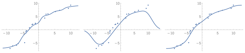
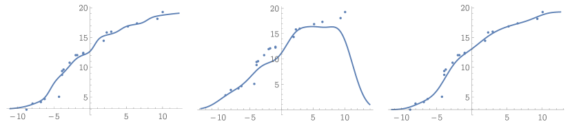
Figure 1: Upper row: graphs of $\hat{f}^{\mathsf{\,NW}}_{K;{\mathbf{x}},{\mathbf{y}}}$ (left), $\hat{f}^{\mathsf{\,PC}}_{K;{\mathbf{x}},{\mathbf{y}}}$ (middle), and $\hat{f}^{\mathsf{\,GM}}_{K;{\mathbf{x}},{\mathbf{y}}}$ (right) for ${\mathbf{x}}$ and ${\mathbf{y}}$ as in (1.9) and (1.10). Lower row: graphs of $\hat{f}^{\mathsf{\,NW}}_{K;{\mathbf{x}},{\mathbf{y}}+\mathbf{10}}$ (left), $\hat{f}^{\mathsf{\,PC}}_{K;{\mathbf{x}},{\mathbf{y}}+\mathbf{10}}$ (middle), and $\hat{f}^{\mathsf{\,GM}}_{K;{\mathbf{x}},{\mathbf{y}}+\mathbf{10}}$ (right) for ${\mathbf{x}}$ and ${\mathbf{y}}$ as in (1.9) and (1.10). Here $K$ is of the form (1.2) with $\kappa$ being the standard normal density.

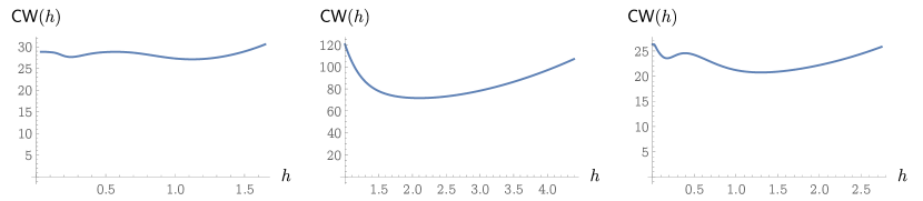
Figure 2: Graphs of $\mathsf{\,CW}$ for the NW estimator (left), the PC estimator (middle), and the GM estimator (right) for ${\mathbf{x}}$ and ${\mathbf{y}}$ as in (1.9) and (1.10). Here $K$ is of the form (1.2) with $\kappa$ being the standard normal density.

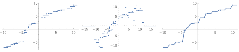
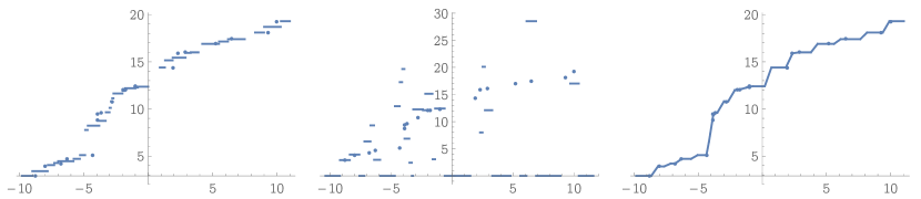
Figure 3: Upper row: graphs of $\hat{f}^{\mathsf{\,NW}}_{K;{\mathbf{x}},{\mathbf{y}}}$ (left), $\hat{f}^{\mathsf{\,PC}}_{K;{\mathbf{x}},{\mathbf{y}}}$ (middle), and $\hat{f}^{\mathsf{\,GM}}_{K;{\mathbf{x}},{\mathbf{y}}}$ (right) for ${\mathbf{x}}$ and ${\mathbf{y}}$ as in (1.9) and (1.10). Lower row: graphs of $\hat{f}^{\mathsf{\,NW}}_{K;{\mathbf{x}},{\mathbf{y}}+\mathbf{10}}$ (left), $\hat{f}^{\mathsf{\,PC}}_{K;{\mathbf{x}},{\mathbf{y}}+\mathbf{10}}$ (middle), and $\hat{f}^{\mathsf{\,GM}}_{K;{\mathbf{x}},{\mathbf{y}}+\mathbf{10}}$ (right) for ${\mathbf{x}}$ and ${\mathbf{y}}$ as in (1.9) and (1.10). Here $K$ is of the form (1.2) with $\kappa$ being the uniform density on $(-1/2,1/2)$.

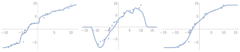
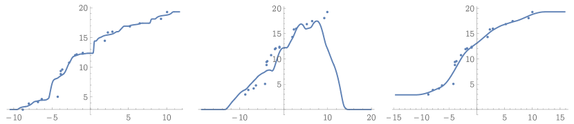
Figure 4: Upper row: graphs of $\hat{f}^{\mathsf{\,NW}}_{K;{\mathbf{x}},{\mathbf{y}}}$ (left), $\hat{f}^{\mathsf{\,PC}}_{K;{\mathbf{x}},{\mathbf{y}}}$ (middle), and $\hat{f}^{\mathsf{\,GM}}_{K;{\mathbf{x}},{\mathbf{y}}}$ (right) for ${\mathbf{x}}$ and ${\mathbf{y}}$ as in (1.9) and (1.10). Lower row: graphs of $\hat{f}^{\mathsf{\,NW}}_{K;{\mathbf{x}},{\mathbf{y}}+\mathbf{10}}$ (left), $\hat{f}^{\mathsf{\,PC}}_{K;{\mathbf{x}},{\mathbf{y}}+\mathbf{10}}$ (middle), and $\hat{f}^{\mathsf{\,GM}}_{K;{\mathbf{x}},{\mathbf{y}}+\mathbf{10}}$ (right) for ${\mathbf{x}}$ and ${\mathbf{y}}$ as in (1.9) and (1.10). Here $K$ is of the form (1.2) with $\kappa(u)=b\,e^{-1/(1-u^{2})}\operatorname{\mathsf{I}}\{|u|<1\}$ for all real $u$, where $b=1/\int_{-1}^{1}e^{-1/(1-u^{2})}\,du$.

2 Discussion

The monotonicity preservation property appears to be natural and desirable for a curve estimator. This is a consequence of the general principle that it is desirable for the values of a statistical estimator to be in the set of all values of the estimated function of the unknown distribution. E.g., it is natural to want the values of an estimator of a nonnegative parameter to be nonnegative; the values of an estimator of a pdf to be pdf’s; etc.

In the rest of the section, we discuss settings where the co-monotonicity condition either holds naturally or is customarily created, and where therefore the monotonicity preservation property is of value.

2.1 Regression settings

In regression settings, where, for each $i\in[n]$, the pair of numbers $(x_{i},y_{i})$ represents the observed/measured values of certain two characteristics of the $i$th individual/sample item, the co-monotonicity condition will hardly ever hold, especially when the sample size $n$ is not too small. Yet, as pointed out by Hall and Huang [9], even in such settings, “Monotone estimates are of course required in many practical applications, where physical considerations suggest that a response should be monotone in the dosage or the explanatory variable.”

There are two kinds of methods to obtain a smooth monotone curve estimator in regression settings:

1. the IS methods: first isotonizing/monotonizing the raw regression data $\big{(}(x_{1},y_{1}),\dots,(x_{n},y_{n})\big{)}$ to satisfy the co-monotonicity condition and then smoothing the monotonized data via (say) a kernel estimator;

2. the SI methods: first smoothing the raw, non-monotonized regression data via (say) a kernel estimator and then isotonizing/monotonizing the output of the smoothing step.

Mammen [14] showed that, under general and rather common conditions, the IS and SI estimators are first-order equivalent to each other in terms of certain estimation errors, with the PC estimator used for the smoothing step. Somewhat similar results, in a more general setting and for a different kind of estimation errors were obtained by Lopuhaä and Musta [13], also with a PC-type smoothing estimator.

However, for the IS estimator to output a monotone curve, the kernel estimator used for the second, smoothing step of the IS procedure must have the monotonicity preservation property. As shown in Theorem 2, the PC estimator never preserves the monotonicity. This calls for results similar to those in [14, 13], but for the NW and GM estimators in place of the PC one; a near-commutativity, IS$\,\approx\,$SI, of the I- and S-operators can be expected for the NW and GM estimators as well. In fact, the first-order asymptotics of an estimation error for the IS estimator using, for the smoothing step, the NW estimator with the symmetric rectangular kernel was obtained already by Mukerjee [15, Theorem 4.2]. Related results for a current status model were given by Groeneboom, Jongbloed, and Witte [8].

One can also note that the IS methods appear to be computationally easier, because in an IS procedure, in contrast with an SI one, the I step is applied to a finite data set; in particular, compare formulas (2.5) and (2.6) in [14] for the I-steps in the IS and and SI procedures, respectively.

Isotonization of raw data $\big{(}(x_{1},y_{1}),\dots,(x_{n},y_{n})\big{)}$ goes back at least to Brunk (see e.g. [2]) and Grenander [7]. A general framework for Grenander-type estimators, including rates of convergence, has been given recently by Westling and Carone [21].

2.2 Matchings

The co-monotonicty condition holds naturally e.g. in the following kind of settings: We have two groups – labeled, say, as an $x$-group and a $y$-group, each consisting of $n$ individuals/items. The items in the $x$-group are ordered according to the values of a certain numerical characteristic, say the $x$-characteristic. Similarly, the items in the $y$-group are ordered according to the values of a certain numerical $y$-characteristic, possibly different from the $x$-characteristic. Then the item in the $x$-group with the $i$th smallest value $x_{i}$ of the $x$-characteristic is matched with the $i$th smallest value $y_{i}$ of the $y$-characteristic in the $y$-group. Then, of course, the co-monotonicity conditions (1.5) and (1.7) will hold. (On the other hand, regression models such as (1.1) are not applicable in “matching” settings.)

For instance, let, as usual, $x_{n:i}$ denote the $i$th smallest value among the values $x_{1},\dots,x_{n}$ of an iid sample from the distribution over $\mathbb{R}$ with a cdf $F$; that is, $x_{n:i}$ is the value of the $i$th order statistic. Matching then the $x_{n:i}$’s with the corresponding $i/n$’s, we obtain the representation $\big{(}(x_{n:1},1/n),\dots,(x_{n:n},n/n)\big{)}$ of the corresponding empirical distribution function. Clearly, the co-monotonicity condition then holds: $x_{n:1}\leqslant\dots\leqslant x_{n:n}$ and $1/n\leqslant\dots\leqslant n/n$. So, smoothing the discrete graph $\big{(}(x_{n:1},1/n),\dots,(x_{n:n},n/n)\big{)}$ by means of a monotonicity-preserving kernel estimator, we obtain a smooth nondecreasing estimate of the cdf $F$.

One can similarly use the inverse discrete graph $\big{(}(1/n,x_{n:1}),\dots,(n/n,x_{n:n})\big{)}$ to obtain a smooth nondecreasing estimate of the quantile function $F^{-1}$ given, say, by the formula $F^{-1}(u):=\min\{x\in\mathbb{R}\colon F(x)\geqslant u\}$ for $u\in(0,1)$. Examples of data of a form similar to that of $\big{(}(1/n,x_{n:1}),\dots,(n/n,x_{n:n})\big{)}$ are, say, household income percentiles data; see e.g. such data for the UK [6] and the US [10].

Let now $y_{n:i}$ denote the $i$th smallest value among the values $y_{1},\dots,y_{n}$ of an iid sample from the distribution over $\mathbb{R}$ with a cdf $G$, possibly different from the cdf $F$. Matching then the order statistics values $x_{n:1},\dots,x_{n:n}$ with the corresponding values $y_{n:1},\dots,y_{n:n}$, we obtain the (automatically co-monotonic) representation $\big{(}(x_{n:1},y_{n:1}),\dots,(x_{n:n},y_{n:n})\big{)}$ of a Q-Q (quantile-quantile) plot for the cdf’s $F$ and $G$. So, applying a monotonicity-preserving smoothing kernel estimator to this Q-Q plot, we obtain a smooth nondecreasing estimate of the “theoretical quantile-quantile function” $G^{-1}\circ F$. In particular, this way we can obtain a smooth monotonic plot of the US household income percentiles against the corresponding percentiles for the UK; similar graphical comparisons can of course be made between, say, different strata/categories of a population.

Yet another example in this vein concerns point processes; see e.g. [11]. For a real $T>0$, let $\xi$ be a point process on the interval $[0,T]$, that is, an integer-valued (nonnegative) random measure on the Borel $\sigma$-algebra over $[0,T]$, so that $\xi=\sum_{i=1}^{N}\delta_{X_{i}}$ for some nonnegative integer-valued r.v. $N$ and some r.v.’s $X_{i}$ with values in $[0,T]$, where $\delta_{a}$ denotes the Dirac probability measure at a point $a$. Let $n,x_{1},\dots,x_{n}$ be sample values/realizations of $N,X_{1},\dots,X_{n}$, respectively. Then $x_{n:1},\dots,x_{n:n}$ can be interpreted as the consecutive times of the occurrences of the “events” of the point process, and the co-monotonicity condition will obviously hold for the data $\big{(}(x_{n:1},1),\dots,(x_{n:n},n)\big{)}$. Smoothing such data by means of a monotonicity-preserving kernel estimator, we obtain a smooth nondecreasing function $\hat{f}$ that is an estimate of the cumulative intensity function $\Lambda_{\xi}$ of the point process $\xi$, given by the formula $\Lambda_{\xi}(t):=\operatorname{\mathsf{E}}\xi([0,t])$ for $t\in[0,T]$; then the derivative $\hat{f}^{\prime}$ of $\hat{f}$ may serve as an estimate of the intensity function $\lambda_{\xi}:=\Lambda^{\prime}_{\xi}$ of the point process $\xi$. Of course, to improve the quality of such estimation, instead of just one realization of the point process one can use a number of such realizations if they are available.

3 Proofs

The proofs of Theorems 1, 2, and 3 given below are each based on quite different ideas.

Proof of Theorem 1.

Consider first the “if” part. Here we suppose that $K$ is log concave. Take any $x$ and $z$ in $D^{\mathsf{\,NW}}_{K;{\mathbf{x}},{\mathbf{y}}}$ such that $x<z$. We have to show that $\hat{f}^{\mathsf{\,NW}}_{K}(z)\geqslant\hat{f}^{\mathsf{\,NW}}_{K}(x)$. Letting for brevity

$$k_{i}:=K(x-x_{i})\quad\text{and}\quad l_{i}:=K(z-x_{i}),$$

$\sum_{i}:=\sum_{i\in[n]}$, and $\sum_{i,j}:=\sum_{i\in[n],j\in[n]}$, we see that

$$2\big{(}\hat{f}^{\mathsf{\,NW}}_{K}(z)-\hat{f}^{\mathsf{\,NW}}_{K}(x)\big{)}\sum_{i}k_{i}\sum_{j}l_{j}$$ (3.1)

$$=2\Big{(}\frac{\sum_{j}y_{j}l_{j}}{\sum_{j}l_{j}}-\frac{\sum_{i}y_{i}k_{i}}{\sum_{i}k_{i}}\Big{)}\sum_{i}k_{i}\sum_{j}l_{j}$$

$$=2\sum_{j}y_{j}l_{j}\sum_{i}k_{i}-2\sum_{i}y_{i}k_{i}\sum_{j}l_{j}$$

$$=\sum_{j}y_{j}l_{j}\sum_{i}k_{i}+\sum_{i}y_{i}l_{i}\sum_{j}k_{j}-\sum_{i}y_{i}k_{i}\sum_{j}l_{j}-\sum_{j}y_{j}k_{j}\sum_{i}l_{i}$$

$$=\sum_{i,j}(y_{j}l_{j}k_{i}+y_{i}l_{i}k_{j}-y_{i}k_{i}l_{j}-y_{j}k_{j}l_{i})$$

$$=\sum_{i,j}(y_{j}-y_{i})(l_{j}k_{i}-k_{j}l_{i}).$$

For any $i$ and $j$ in $[n]$ such that $i\leqslant j$ we have $x_{i}\leqslant x_{j}$ and hence, by the log-concavity of $K$, $k_{i}\geqslant l_{i}^{1-t}k_{j}^{t}$ and $l_{j}\geqslant l_{i}^{t}k_{j}^{1-t}$, where $t:=t_{i,j}:=(z-x)/(x_{j}-x_{i}+z-x)\in[0,1)$ and $0^{0}:=0$, so that $l_{j}k_{i}\geqslant k_{j}l_{i}$ and hence $(y_{j}-y_{i})(l_{j}k_{i}-k_{j}l_{i})\geqslant 0$. The latter inequality similarly holds for any $i$ and $j$ in $[n]$ such that $i\geqslant j$. So, by (3.1), we have $\hat{f}^{\mathsf{\,NW}}_{K}(z)\geqslant\hat{f}^{\mathsf{\,NW}}_{K}(x)$, which completes the proof of the “if” part of Theorem 1.

Consider now the “only if” part of Theorem 1. Here we are assuming that the NW kernel estimator preserves the monotonicity for $K$, and we have to show that $K$ is then log concave. It is enough to show that $K$ is log concave on the set $s(K):=\{x\in\mathbb{R}\colon K(x)>0\}$.

Take $n=2$, $y_{1}=0$, $y_{2}=1$, $x_{1}=0$, $x_{2}=(v-u)/2$, $x=(v+u)/2$, and $z=v$ for any $u$ and $v$ in $s(K)$ such that $u<v$. Then, by (3.1), $l_{2}k_{1}\geqslant k_{2}l_{1}$, that is, $K((v+u)/2)^{2}\geqslant K(u)K(v)$, which means that $\ln K$ is midpoint concave. Also, $\ln K$ is Lebesgue measurable, since $K$ is a pdf. By Sierpiński’s theorem [18], any Lebesgue measurable midpoint concave function is concave. So, $\ln K$ is concave and thus $K$ is log concave. Now the “only if” part of Theorem 1 is proved as well. ∎

Proof of Theorem 2.

Take any kernel $K$, any natural $n$, and any co-monotone ${\mathbf{x}}$ and ${\mathbf{y}}$ in $\mathbb{R}^{n}$ such that the function $\hat{f}^{\mathsf{\,PC}}_{K;{\mathbf{x}},{\mathbf{y}}}$ is nondecreasing. We have to show that then ${\mathbf{x}}$ and ${\mathbf{y}}$ are trivial in the sense that (1.8) holds.

Since $K$ is a pdf, (1.4) implies

$$\int_{\mathbb{R}}\hat{f}^{\mathsf{\,PC}}_{K}(x)\,dx:=\sum_{i=1}^{n}y_{i}\,(x_{i}-x_{i-1})\in\mathbb{R},$$

so that $\int_{\mathbb{R}}\hat{f}^{\mathsf{\,PC}}_{K}\in L^{1}(\mathbb{R})$.

However, the only nondecreasing function $f\in L^{1}(\mathbb{R})$ is the zero function. Indeed, if $f(a)>0$ for some $a\in\mathbb{R}$, then $f\geqslant f(a)>0$ on the interval $[a,\infty)$ and hence $\int_{[a,\infty)}f(x)\,dx=\infty$, which contradicts the assumption $f\in L^{1}(\mathbb{R})$. Similarly, if $f(a)<0$ for some $a\in\mathbb{R}$, then $f\leqslant f(a)<0$ on the interval $(-\infty,a]$ and hence $\int_{(-\infty,a]}f(x)\,dx=-\infty$, which again contradicts the assumption $f\in L^{1}(\mathbb{R})$.

Therefore and because the function $\hat{f}^{\mathsf{\,PC}}_{K;{\mathbf{x}},{\mathbf{y}}}$ was assumed to be nondecreasing, we conclude that $\hat{f}^{\mathsf{\,PC}}_{K;{\mathbf{x}},{\mathbf{y}}}$ must be the zero function. Recalling (1.4) again and applying the Fourier transform, we see that

$$\sum_{j=1}^{n}y_{j}\,(x_{j}-x_{j-1})e^{itx_{j}}\hat{K}(t)=0$$ (3.2)

for all real $t$, where $\hat{K}$ is the Fourier transform/characteristic function of the pdf $K$ given by the formula

$$\hat{K}(t):=\int_{\mathbb{R}}e^{itx}K(x)\,dx$$

and $i$ is the imaginary unit. Since $\hat{K}(0)=1$ and the function $\hat{K}$ is continuous, there exists some real $t_{0}>0$ such that for all $t\in(-t_{0},t_{0})$ we have $\hat{K}(t)\neq 0$ and hence, by (3.2), $\sum_{j=1}^{n}y_{j}\,(x_{j}-x_{j-1})e^{itx_{j}}=0$ or, equivalently,

$$\sum_{j\in J}y_{j}\,(x_{j}-x_{j-1})e^{itx_{j}}=0,$$

where

$$J:=\big{\{}j\in\{1,\dots,n\}\colon x_{j}-x_{j-1}\neq 0\big{\}}.$$

Note that the $x_{j}$’s for $j\in J$ are pairwise distinct – because for any $j$ and $k$ in $J$ such that $j<k$ we have $x_{j}\leqslant x_{k-1}<x_{k}$. Using now the textbook fact that exponential functions are linearly independent on any nonempty open interval (cf. e.g. Lemma 3.2 on page 92 in [3] or a more general version for group characters [1, Theorem 12, page 38]), we conclude that $y_{j}\,(x_{j}-x_{j-1})=0$ for all $j\in J$ and hence for all $j\in\{1,\dots,n\}$, which completes the proof of Theorem 2. ∎

Proof of Theorem 3.

Let $F$ be the cdf corresponding to the pdf $K$, so that

$$F(x)=\int_{-\infty}^{x}K(u)\,du$$

for $x\in[-\infty,\infty]$. Also introduce

$$(\Delta_{i}F)(x):=F(x-s_{i-1})-F(x-s_{i})$$

for all $x\in[-\infty,\infty]$ and all $i=1,\dots,n$ and

$$\Delta y_{i}:=y_{i}-y_{i-1}$$

for all $i=2,\dots,n$, so that

$$y_{i}=y_{1}+\sum_{j=2}^{i}\Delta y_{j}$$

for all $i=1,\dots,n$; as usual, $\sum_{j=2}^{1}\dots:=0$. Then, recalling the definition (1.6) of the GM kernel estimator, for all real $x$ we have

$$\hat{f}^{\mathsf{\,GM}}_{K}(x) =\sum_{i=1}^{n}y_{i}\,(\Delta_{i}F)(x)$$

$$=\sum_{i=1}^{n}\Big{(}y_{1}+\sum_{j=2}^{i}\Delta y_{j}\Big{)}(\Delta_{i}F)(x)$$

$$=y_{1}\sum_{i=1}^{n}(\Delta_{i}F)(x)+\sum_{i=1}^{n}\sum_{j=2}^{i}\Delta y_{j}\,(\Delta_{i}F)(x)$$

$$=y_{1}+\sum_{j=2}^{n}\Delta y_{j}\,\sum_{i=j}^{n}(\Delta_{i}F)(x)$$

$$=y_{1}+\sum_{j=2}^{n}\Delta y_{j}\,F(x-s_{j-1}),$$

taking into account that $s_{0}=-\infty$ and $s_{n}=\infty$, whereas $F(-\infty)=0$ and $F(\infty)=1$. Also, by (1.7), $\Delta y_{j}\geqslant 0$ for all $j=2,\dots,n$. Now it is obvious that the function $\hat{f}^{\mathsf{\,GM}}_{K}$ is nondecreasing. This completes the proof of Theorem 3. ∎

References

- [1] Emil Artin, Galois theory, Edited and supplemented with a section on applications by Arthur N. Milgram. Second edition, with additions and revisions. Fifth reprinting. Notre Dame Mathematical Lectures, No. 2, University of Notre Dame Press, South Bend, Ind., 1959. MR 0265324
- [2] Miriam Ayer, H. D. Brunk, G. M. Ewing, W. T. Reid, and Edward Silverman, An empirical distribution function for sampling with incomplete information, Ann. Math. Statist. 26 (1955), 641–647. MR 73895
- [3] Viorel Barbu, Differential equations, Springer, Cham, 2016. MR 3585801
- [4] C.-K. Chu and J. S. Marron, Choosing a kernel regression estimator, Statist. Sci. 6 (1991), no. 4, 404–436, With comments and a rejoinder by the authors. MR 1146907
- [5] Theo Gasser and Hans-Georg Müller, Kernel estimation of regression functions, Smoothing techniques for curve estimation (Proc. Workshop, Heidelberg, 1979), Lecture Notes in Math., vol. 757, Springer, Berlin, 1979, pp. 23–68. MR 564251
- [6] UK Government, Percentile points from 1 to 99 for total income before and after tax, https://www.gov.uk/government/statistics/percentile-points-from-1-to-99-for-total-income-before-and-after-tax, 2020, [Online; accessed 21-January-2021].
- [7] Ulf Grenander, On the theory of mortality measurement. II, Skand. Aktuarietidskr. 39 (1956), 125–153 (1957). MR 93415
- [8] Piet Groeneboom, Geurt Jongbloed, and Birgit I. Witte, Maximum smoothed likelihood estimation and smoothed maximum likelihood estimation in the current status model, Ann. Statist. 38 (2010), no. 1, 352–387. MR 2589325
- [9] Peter Hall and Li-Shan Huang, Nonparametric kernel regression subject to monotonicity constraints, Ann. Statist. 29 (2001), no. 3, 624–647. MR 1865334
- [10] Don’t Quit Your Day Job, Average, Median, Top 1%, and all United States Household Income Percentiles in 2020, https://dqydj.com/average-median-top-household-income-percentiles/, 2020, [Online; accessed 21-January-2021].
- [11] Olav Kallenberg, Random measures, third ed., Akademie-Verlag, Berlin; Academic Press, Inc. [Harcourt Brace Jovanovich, Publishers], London, 1983. MR 818219
- [12] E. L. Lehmann, Testing statistical hypotheses, John Wiley & Sons, Inc., New York; Chapman & Hall, Ltd., London, 1959. MR 0107933
- [13] Hendrik P. Lopuhaä and Eni Musta, Central limit theorems for the -error of smooth isotonic estimators, Electron. J. Stat. 13 (2019), no. 1, 1031–1098. MR 3935844
- [14] Enno Mammen, Estimating a smooth monotone regression function, Ann. Statist. 19 (1991), no. 2, 724–740. MR 1105841
- [15] Hari Mukerjee, Monotone nonparameteric regression, Ann. Statist. 16 (1988), no. 2, 741–750. MR 947574
- [16] E. A. Nadaraya, On nonparametric estimates of density functions and regression curves, Theory Probab. Appl. 10 (1965), 186–190.
- [17] M. B. Priestley and M. T. Chao, Non-parametric function fitting, J. Roy. Statist. Soc. Ser. B 34 (1972), 385–392. MR 331616
- [18] Waclaw Sierpinski, Sur les fonctions convexes mesurables, Fundamenta Mathematicae 1 (1920), no. 1, 125–128.
- [19] M. Stone, Cross-validatory choice and assessment of statistical predictions, Journal of the Royal Statistical Society. Series B (Methodological) 36 (1974), no. 2, 111–147.
- [20] Geoffrey S. Watson, Smooth regression analysis, Sankhyā Ser. A 26 (1964), 359–372. MR 185765
- [21] Ted Westling and Marco Carone, A unified study of nonparametric inference for monotone functions, Ann. Statist. 48 (2020), no. 2, 1001–1024. MR 4102685