On coalescence as the origin of nuclei in hadronic collisions

Abstract

The origin of weakly-bound nuclear clusters in hadronic collisions is a key question to be addressed by heavy-ion collision (HIC) experiments. The measured yields of clusters are approximately consistent with expectations from phenomenological statistical hadronisation models (SHMs), but a theoretical understanding of the dynamics of cluster formation prior to kinetic freeze out is lacking. The competing model is nuclear coalescence, which attributes cluster formation to the effect of final state interactions (FSI) during the propagation of the nuclei from kinetic freeze out to the observer. This phenomenon is closely related to the effect of FSI in imprinting femtoscopic correlations between continuum pairs of particles at small relative momentum difference. We give a concise theoretical derivation of the coalescence–correlation relation, predicting nuclear cluster spectra from femtoscopic measurements. We review the fact that coalescence derives from a relativistic Bethe-Salpeter equation, and recall how effective quantum mechanics controls the dynamics of cluster particles that are nonrelativistic in the cluster centre of mass frame. We demonstrate that the coalescence–correlation relation is roughly consistent with the observed cluster spectra in systems ranging from PbPb to pPb and pp collisions. Paying special attention to nuclear wave functions, we derive the coalescence prediction for hypertriton and show that it, too, is roughly consistent with the data. Our work motivates a combined experimental programme addressing femtoscopy and cluster production under a unified framework. Upcoming pp, pPb and peripheral PbPb data analysed within such a programme could stringently test coalescence as the origin of clusters.

I Introduction

Loosely-bound nuclei like the D, ³He, ³H, ${}^{3}_{\Lambda}$H and their anti-particles are detected among the products of high-energy hadronic collisions at the large hadron collider (LHC) and other experiments, and their study is a central objective in heavy-ion collision (HIC) experiments Csernai and Kapusta (1986); Andronic et al. (2011); Cleymans et al. (2011). Interestingly, the momentum-integrated yields of these nuclei are roughly consistent with being drawn from a thermal distribution with the same temperature parameter $T_{ch}$ that fits the yields of mesons and nucleons Andronic et al. (2018); Vovchenko et al. (2018, 2019); Acharya et al. (2018a). Taken together from $\pi^{\pm}$ to ⁴He, the hadron yields span some $\sim 9$ orders of magnitude with only $\mathcal{O}(1)$ discrepancies. This has led some authors to speculate that nuclei take part, on equal footing with the “more fundamental” mesons and nucleons, in an equilibrium partition function characterising the high excitation state (HXS) produced in HICs. A recent account of this statistical hadronisation model (SHM) is given in Andronic et al. (2018).

While the SHM is approximately consistent with cluster yields, no first-principle theoretical framework as of yet explains the dynamics of cluster formation in the HXS before kinetic freeze out. Clusters are big (several fm) fragile (binding energies $E_{b}\lesssim 10$ MeV, as low as $E_{b}\sim 0.13$ MeV for ${}^{3}_{\Lambda}$H Juric et al. (1973)) objects, while even at kinetic freeze out the HXS does not exceed a few fm and it is a hot state with characteristic particle excitation energies of $\sim 100$ MeV. What does it mean for a D with diameter $\sim 4$ fm to exist in an equilibrium distribution in an HXS of diameter $\sim 2$ fm, produced in pp collisions? What does it mean for ${}^{3}_{\Lambda}$H, with effective diameter $\sim 14$ fm? This puzzle makes the origin of nuclei uniquely interesting.

The kinetic theory analysis of Oliinychenko et al. (2019), focusing on D formation in high-multiplicity PbPb collisions, may shed some light on the problem. This analysis demonstrated that, indeed, D observed at the detector must emerge from the kinetic freeze out region and not from the chemical freeze out region of the HXS, to which the SHM parameter $T_{ch}$ corresponds. However, Ref. Oliinychenko et al. (2019) treated the D as a point-particle and it is far from clear if and how their analysis could be adapted to smaller systems like pp, pPb or peripheral PbPb collisions.

An alternative explanation for the origin of nuclei, bypassing the limitations of kinetic theory, is proposed by coalescence. The basic assumption of the coalescence model is that the expansion of the HXS leads to kinetic freeze out with nucleons but – due to their fragility and size – essentially no nuclei. The HXS at kinetic freeze out can be described by a quantum mechanical (QM) density matrix. Projecting the density matrix onto particle states at the detector gives the observed particle spectra. Final state interactions (FSI) mediated by nuclear scattering and Coulomb photon exchange enter this projection as they affect the propagation of the particles from the HXS to the detector. FSI manifest themselves in two ways:

1. FSI imprint momentum correlations among pairs of continuum particles. The analysis of this phenomenon is known as femtoscopy or Hanbury Brown-Twiss (HBT) analysis.

2. FSI also admit discrete bound-state multi-nucleon solutions, namely nuclei. This is nuclear coalescence.

It is important to note that the coalescence model predicts that the yields of nuclei approximately inherit the thermal spectra of their nucleon constituents, up to a dimensionless QM correction factor. In many cases (e.g. low-$p_{t}$ D and ³He formation in high multiplicity PbPb collisions) the QM correction factor is close to unity Csernai and Kapusta (1986); Scheibl and Heinz (1999). Thus, the approximately thermal yield of nuclei need not point to the nuclei taking part in an equilibrium partition function before kinetic freeze out. For some nuclei and systems, however, the QM factor is predicted to be much smaller than unity. An example is the production of ${}^{3}_{\Lambda}$H in pp collisions, or (especially at high-$p_{t}$) in low multiplicity PbPb collisions. These systems offer a key discriminator between the coalescence model and the SHM. Our goal in this paper is to study the theoretical prediction of coalescence, compare to available experimental data and highlight the path to making this test conclusive.

A central feature in this paper is the relation between coalescence and HBT correlations among continuum nucleons. From the perspective of the coalescence model, HBT correlations and nuclei production are closely related. In a clear sense, the successful reconstruction of the imprint of FSI on pair correlations lends credence to the basic framework of coalescence, which deals with the bound state solutions of essentially the same FSI (in different isospin channels). Moreover, once HBT calibrates the HXS source characteristics, nuclei yields are predicted without free parameters. Over the years the community (experimental and theoretical) developed a habit of considering HBT and nuclei analyses separately, making it cumbersome to combine the information content of the measurements. One of our goals here is to motivate joint experimental analyses of HBT and cluster yields.

The plan of the paper, along with a brief summary, are as follows.

In Sec. II we briefly review the underlying relation between femtoscopy and cluster formation, defining the coalescence/femtoscopy framework. The basic formalism was laid out by Lednicky et al Lednicky and Lyuboshits (1982); Akkelin et al. (2002); Lednicky (2009). We provide a quick reduction of this formalism to observationally accessible objects. This is a good starting point for the discussion, because it demonstrates that coalescence arises in a relativistic quantum field theoretic (QFT) calculation. In Sec. II.1 we show how, subject to two key approximations (the smoothness approximation and the equal-time approximation), the model-independent coalescence–correlation relation between deuteron production and two-proton HBT comes about. The main result here is the manifest relation between the well-known Eq. (14), for HBT, and Eq. (15), for the D coalescence factor. This relation was derived first in Blum and Takimoto (2019) starting from the QM limit. Our independent derivation here gives another perspective on this result, showing, for example, that it does not require density matrix factorisation to apply for its validity. In Sec. II.2 we review how adding the assumption of density matrix factorisation allows one to connect two-particle HBT analyses to single-particle spectra and three-body coalescence. In Sec. II.2.2 we derive the coalescence prediction for ${}_{\Lambda}^{3}$H and ³He. Eqs. (30,31), or their momentum space versions of Eqs. (34,35), are the most model-independent versions of these coalescence factors we know of.

None of our results in Sec. II rely on the details of the underlying nucleon emission function, or needs to specify a model of the dynamical evolution of the HXS: our results simply connect femtoscopy with cluster yields, and the connection should apply to any self-consistent HXS model. To make contact with measurements, however, we need to specify the two- and three-particle source. We turn to this in Sec. III. We start in Sec. III.1 by appealing to observational HBT parameterisations of the two-particle source (extended, with some added assumptions, to the three-particle source). Relying on experimental fits allows us to keep the analysis as model-independent as we can. While this is not an essential requirement of the framework, we stick in this paper to Gaussian or semi-Gaussian parameterisations. In Apps. A and B we give some quantitative model-dependent theoretical examples that suggest that an anisotropic (3D) Gaussian source parameterisation is probably accurate enough for the purpose of testing the origin of clusters via the coalescence–correlations relation.

The next ingredient needed is the nuclear wave functions. In Sec. III.2 we derive the coalescence factors corresponding to the simplified Gaussian wave functions. The Gaussian wave function is an over-simplification in some cases, but at the cost of an $\mathcal{O}(1)$ theoretical error it allows us to derive analytic results for the coalescence factors, summarised by Eqs. (49,50,51). We note that the Gaussian wave functions we consider allow for different cluster length scales for three-body states; for ${}_{\Lambda}^{3}$H this is crucial, as the p-n factor of the wave function is considerably more compact than the $\Lambda$-pn factor. Eqs. (49,50,51) also account for the intrinsically anisotropic shape of the two- and three-particle source describing the HXS. As we illustrate in App. B, the two-particle source is expected to be truly anisotropic, especially at large $p_{t}$.

In Sec. III.3 we extend the analysis to more accurate non-Gaussian wave functions. For D we derive an analytic coalescence factor formula that applies to the Hulthen wave function if the underlying two-particle source is approximated as 1D Gaussian. The more realistic 3D two-particle source can be easily accounted for by numerical integration. For ${}_{\Lambda}^{3}$H we consider the recent three-body wave function proposed by Hildenbrand and Hammer (2019). We show that while the theoretically expected wave function is non-Gaussian, exhibiting an extended high-$q$ tail, nevertheless an effective Gaussian wave function fit does a reasonably accurate job in the coalescence factor calculation (valid to a factor of $\sim 2$). What does turn out – as already noted above – to be quantitatively important, is the consideration of the two different length scales associated with the p-n and $\Lambda$-pn factors of the state.

In Sec. IV we give a rudimentary comparison to data. In Sec. IV.1 we recap results from Blum and Takimoto (2019) for D and ³He, adding a pPb data point to the PbPb and pp measurements discussed there; we also correct a few typos in Blum and Takimoto (2019). In Sec. IV.2 we compare the coalescence prediction for ${}^{3}_{\Lambda}$H to PbPb data. We emphasise (as was done before us Zhang and Ko (2018); Sun et al. (2019); Bellini and Kalweit (2019); but here with a robust coalescence calculation) that ${}^{3}_{\Lambda}$H data in small systems (pp, pPb, or low multiplicity PbPb) has the potential to conclusively rule out (or support) coalescence as the dominant origin of clusters.

In Sec. V we discuss and summarise our results.

II The coalescence/femtoscopy framework

The description of femtoscopic correlations between nucleons Koonin (1977) and the coalescence model for nuclei Bond et al. (1977); Sato and Yazaki (1981) are two aspects of the same theoretical framework. The idea is that at kinetic freeze out the HXS can be described by a multi-particle density matrix $\hat{\rho}_{\rm HX}$. Depending on the measured observable, this density matrix can be projected onto final states of different multiplicities. In what follows we present a concise derivation of coalescence and the coalescence–correlations relation Blum and Takimoto (2019), aiming to collect different aspects of the problem under the same roof, so to speak. Many of the results were also derived elsewhere, notably in Lednicky and Lyuboshits (1982); Akkelin et al. (2002); Lednicky (2009); Blum and Takimoto (2019) and (albeit with model-dependence) in Mrowczynski (1987, 1990, 1992, 1993, 1995); Maj and Mrowczynski (2005); Mrowczynski (2017); Scheibl and Heinz (1999); Blum et al. (2017).

II.1 Two-particle correlations and the deuteron.

If the phase space density of nucleons around the time when they last scatter against other particles (mostly pions) in the HXS is not too high, then the subsequent propagation of pairs of nucleons emitted very near in phase space would be dominated by FSI, while additional interactions with particles other than the pair would be sub-dominant. With this sudden approximation, the Lorentz-invariant yield of nucleon pairs at total spin $s$ is given by Lednicky and Lyuboshits (1982); Lednicky (2009)

$$\gamma_{1}\gamma_{2}\frac{dN_{2,s}}{d^{3}{\bf p}_{1}d^{3}{\bf p}_{2}} = \frac{2s+1}{(2\pi)^{6}}\int d^{4}x_{1}\int d^{4}x_{2}\int d^{4}x^{\prime}_{1}\int d^{4}x^{\prime}_{2}\,\Psi^{*}_{s,p_{1},p_{2}}(x^{\prime}_{1},x^{\prime}_{2})\,\Psi_{s,p_{1},p_{2}}(x_{1},x_{2})\,\rho_{p_{1},p_{2}}\left(x_{1},x_{2};x^{\prime}_{1},x^{\prime}_{2}\right),$$ (1)

where $\Psi_{s,p_{1},p_{2}}(x_{1},x_{2})$ is the continuum Bethe-Salpeter amplitude Schweber et al. (1955) describing the FSI of the pair. Similarly, the yield of deuterons at momentum $P$ is given by

$$\gamma\frac{dN_{\rm d}}{d^{3}{\bf P}} = \frac{2s_{d}+1}{(2\pi)^{3}}\int d^{4}x_{1}\int d^{4}x_{2}\int d^{4}x^{\prime}_{1}\int d^{4}x^{\prime}_{2}\,\Psi^{*}_{d,P}(x^{\prime}_{1},x^{\prime}_{2})\,\Psi_{d,P}(x_{1},x_{2})\,\rho_{p_{1},p_{2}}\left(x_{1},x_{2};x^{\prime}_{1},x^{\prime}_{2}\right),$$ (2)

where $\Psi_{d,P}(x_{1},x_{2})$ is the bound state Bethe-Salpeter amplitude describing the deuteron. The role of the Bethe-Salpeter amplitudes $\Psi$ is to resum soft diagonal (ladder) FSI diagrams, factoring their effect out of an assumed underlying short-distance amplitude forming the density matrix $\rho_{p_{1},p_{2}}$.

Obviously, modelling the spectra Eqs. (1-2) requires proper modelling of the FSI, that are either calculable from first principles (in the case of Coulomb) or measurable (in the case of nuclear scattering amplitudes) and that we assume to be known. Modelling $\rho_{p_{1},p_{2}}$ from first principles, however, is currently impossible. Our goal in this section, and in the rest of the paper, is to demonstrate that even without a-priori knowledge of $\rho_{p_{1},p_{2}}$, the mere fact that the same $\rho_{p_{1},p_{2}}$ occurs in both of Eqs. (1) and (2) is enough to allow a model-independent, approximate prediction of the deuteron (and, with some added assumptions, other clusters) spectrum based on measurements of HBT correlations Blum and Takimoto (2019).

Let us define $c_{1,2}=(p_{1,2}P)/P^{2}$, where the pair total momentum is $P=p_{1}+p_{2}\,\equiv\,2p$. In general, the dependence of the amplitude $\Psi$ (be it $\Psi_{s,p_{1},p_{2}}$ or $\Psi_{d,P}$) on the pair total momentum and centre of mass coordinate $X=c_{1}x_{1}+c_{2}x_{2}$ can be factored out from the dependence on the relative momentum $q=c_{2}p_{1}-c_{1}p_{2}$ and relative position $x=x_{1}-x_{2}$, via

$$\Psi(x_{1},x_{2}) = e^{-iPX}\phi(x).$$ (3)

Using Eq. (3) and changing to convenient coordinates, we can rewrite Eqs. (1-2) as:

$$\gamma_{1}\gamma_{2}\frac{dN_{2,s}}{d^{3}{\bf p}_{1}d^{3}{\bf p}_{2}} = \frac{2s+1}{(2\pi)^{6}}\int d^{4}{r}\int\frac{d^{4}{k}}{(2\pi)^{4}}\,\tilde{\mathcal{D}}_{s,q}\left({k},{r}\right)\,\tilde{S}_{p_{1},p_{2}}\left({k,r}\right),$$ (4)

$$\gamma\frac{dN_{\rm d}}{d^{3}{\bf P}} = \frac{2s_{d}+1}{(2\pi)^{3}}\int d^{4}{r}\int\frac{d^{4}{k}}{(2\pi)^{4}}\,\tilde{\mathcal{D}}_{d}\left({k},{r}\right)\,\tilde{S}_{p_{1},p_{2}}\left({k,r}\right),$$ (5)

where we define the relativistic internal Wigner density

$$\tilde{\mathcal{D}}\left({k},{r}\right) = \int d^{4}{\zeta}\,e^{i{k}{\bf\zeta}}\,\phi\left({r}+\frac{{\zeta}}{2}\right)\,\phi^{*}\left({r}-\frac{{\zeta}}{2}\right)$$ (6)

(with $\tilde{\mathcal{D}}_{s,q}$ and $\tilde{\mathcal{D}}_{d}$ obtained from $\phi_{s,q}$ and $\phi_{d}$, respectively) and where

$$\tilde{S}_{p_{1},p_{2}}\left({k,r}\right) = \int d^{4}x\int d^{4}l_{1}\,e^{-il_{1}(c_{1}P+k)}\int d^{4}l_{2}\,e^{-il_{2}(c_{2}P-k)}\,\times$$

$$\rho_{p_{1},p_{2}}\left(x+c_{2}r+\frac{l_{1}}{2},x-c_{1}r+\frac{l_{2}}{2};x+c_{2}r-\frac{l_{1}}{2},x-c_{1}r-\frac{l_{2}}{2}\right).$$

The Wigner density we would obtain if we could turn off both FSI and quantum statistics is $\mathcal{D}_{s,q}^{0}(k,r)=(2\pi)^{4}\delta^{(4)}\left(k-q\right)$, independent of $r$. With this we can define a hypothetical reference uncorrelated pair spectrum,

$$\gamma_{1}\gamma_{2}\frac{dN_{2}^{0}}{d^{3}{\bf p}_{1}d^{3}{\bf p}_{2}} = \frac{(2s_{N}+1)^{2}}{(2\pi)^{6}}\int d^{4}{r}\,\tilde{S}_{p_{1},p_{2}}\left(q,r\right),$$ (8)

where $s_{N}=1/2$ is the nucleon spin. The reference pair spectrum is not a real physical object, but we can try to mimic it experimentally by pairing particles from different events with similar event characteristics. With this understanding, the pair correlation function is defined as

$$C(p,q) = \frac{\sum_{s}\gamma_{1}\gamma_{2}\frac{dN_{2,s}}{d^{3}{\bf p}_{1}d^{3}{\bf p}_{2}}}{\gamma_{1}\gamma_{2}\frac{dN_{2}^{0}}{d^{3}{\bf p}_{1}d^{3}{\bf p}_{2}}}$$ (9)

and the coalescence factor for deuteron formation is defined as

$$\mathcal{B}_{2}(p) = \frac{P^{0}\frac{dN_{\rm d}}{d^{3}{\bf P}}}{p^{0}_{1}p^{0}_{2}\frac{dN_{2}^{0}}{d^{3}{\bf p}_{1}d^{3}{\bf p}_{2}}}\;\approx\;\frac{2}{m}\frac{\gamma\frac{dN_{\rm d}}{d^{3}{\bf P}}}{\gamma_{1}\gamma_{2}\frac{dN_{2}^{0}}{d^{3}{\bf p}_{1}d^{3}{\bf p}_{2}}},$$ (10)

where we approximated $m_{D}\approx 2m$.

At this point it is useful to make two approximations:

• Smoothness approximation: The smoothness approximation was discussed widely in the literature Pratt (1997); Heinz and Jacak (1999); Lisa et al. (2005). The version of this approximation we take here amounts to replacing $S_{p_{1},p_{2}}(k,r)\approx S_{p_{1},p_{2}}(0,r)$ in Eqs. (4) and (5). The $k$ integral of the $\tilde{\mathcal{D}}$ functions can then be done, yielding $\int\frac{d^{4}k}{(2\pi)^{4}}\tilde{\mathcal{D}}(k,r)=|\phi(r)|^{2}$. Similarly, we replace $S_{p_{1},p_{2}}(q,r)\approx S_{p_{1},p_{2}}(0,r)$ in the reference pair spectrum Eq. (8). The accuracy of the smoothness approximation is probably sufficient for our purpose in PbPb collisions; in pp collisions we think that a careful assessment is still warranted.

• Equal-time approximation: In the pair rest frame (PRF) we have $P=(M,{\bf 0})$, $q=(0,{\bf q})$ and $x=(t,{\bf x})$. Both for two-particle correlations and bound states, we are interested in pairs that are nonrelativistic in the PRF, ${\bf q}^{2}\ll m^{2}$, and can neglect corrections of $\mathcal{O}({\bf q}^{2}/m^{2})$. A key point, derived clearly in Lednicky and Lyuboshits (1982); Lednicky (2009), is that the Bethe-Salpeter amplitude in the PRF-nonrelativistic limit is approximately independent of the PRF time:

  $$\phi(x) = \phi({\bf x})\left(1+\mathcal{O}\left(\frac{t}{m{\bf x}^{2}}\right)\right).$$ (11)

  At the level of the leading term in the equal-time approximation of Eq. (11), $\phi_{s,q}$ ($\phi_{d}$) is equal to the QM static scattering wave (bound state) solution of the Schrödinger equation Landau and Lifshits (1991).

  In hadronic collisions we have $t\sim{\bf x}\sim$ few fm, implying a correction $\sim 0.2\frac{1\rm fm}{{\bf x}}$ to the equal-time approximation. Thus, we are certainly sacrificing some precision when we adopt it: the incurred theoretical error is probably in the ballpark of 10% for PbPb collisions, where ${\bf x}\sim 3$ fm, but could be several tens of percent in pp collisions where ${\bf x}\sim 1$ fm. Nevertheless, the equal-time approximation would allow us significant mileage with relatively simple notation. We think that it probably allows for sufficient accuracy to establish (or exclude) coalescence as the main origin of clusters in hadronic collisions. Note that the free solution in the absence of FSI is the plane wave $\phi(x)=e^{-iqx}$ [(anti-)symmetrised by QS] and the equal-time limit of Eq. (11) is exact in that case, because in the PRF $qx=-{\bf qx}$.

Adopting the smoothness and equal-time approximations we are led to the definition of the normalised two-particle source $\mathcal{S}_{2}$, a function of the PRF spatial coordinate ${\bf r}$, as an integral in PRF time $t=r^{0}$:

$$\mathcal{S}_{2}({\bf r}) = \frac{\int dr^{0}\tilde{S}_{p_{1},p_{2}}\left({0,r}\right)}{\int d^{4}{r}\,\tilde{S}_{p_{1},p_{2}}\left({0,r}\right)}.$$ (12)

The pair correlation function is then given from Eq. (9) as

$$C(p,q) = \sum_{s}w_{s}C_{s}(p,q)$$ (13)

with the spin weights $w_{s}=(2s+1)/(2s_{N}+1)^{2}$ and

$$C_{s}(p,q) \approx \int d^{3}{\bf r}\,\left|\phi_{s,q}\left({\bf r}\right)\right|^{2}\mathcal{S}_{2}({\bf r}).$$ (14)

Similarly, the deuteron coalescence factor is given from Eq. (10) as

$$\mathcal{B}_{2}(p) \approx \frac{2(2s_{d}+1)}{m(2s_{N}+1)^{2}}(2\pi)^{3}\int d^{3}{\bf r}\,\left|\phi_{d}\left({\bf r}\right)\right|^{2}\,\mathcal{S}_{2}({\bf r}).$$ (15)

Two general comments are in order. First, the aim of HBT analyses like, e.g., Refs. Adam et al. (2015); Acharya et al. (2019a, 2020a) (for reviews, see Lisa et al. (2005); Heinz and Jacak (1999)) is to measure the source $\mathcal{S}_{2}({\bf r})$ by solving the Schrödinger equation for the wave functions $\phi_{s,q}({\bf r})$ Koonin (1977); Lednicky (2009); Mihaylov et al. (2018) and comparing the observed two-particle spectrum with Eqs. (13-14). In this exercise, obtaining agreement with the experimental data appears to require the use of the correct set of FSI potentials. While this point is not often stated explicitly, the success of the source reconstruction analyses lends some credence to the basic framework leading to Eqs. (13-14). As we have just seen, this is the same framework that stands behind the coalescence model for nuclei, the only difference being that HBT deals with continuum scattering state solutions of FSI and coalescence deals with discrete bound state solutions of FSI. Thus the mere existence of successful HBT analyses lends some credence to coalescence as the origin of (at least some of the) nuclei observed in hadronic collisions.

Second, with $\mathcal{S}_{2}({\bf r})$ measured, Eq. (15) predicts the deuteron yield model-independently and with no free parameters. As we show in Sec. IV, this prediction is consistent with experimental data to within a factor of two or so across systems ranging from PbPb to pPb and pp at different multiplicities Blum et al. (2017); Blum and Takimoto (2019). This is strong evidence that coalescence contributes to the production of deuterons in hadronic collisions at the $\mathcal{O}(1)$ level, at least.

A caveat to keep in mind is that although Eq. (14) is commonly used in the literature, we do not know a model-independent way of checking the quantitative corrections due to the smoothness and equal-time approximations, which we have done to reduce Eq. (4) into Eq. (14); nor to the sudden approximation itself, allowing us to write Eq. (4) in the first place. A systematic study of these uncertainties is warranted if one wishes to narrow down the theory uncertainty associated with Eq. (15).

As a technical aside, it is convenient to carry out some of the analysis in momentum space. To this end it is useful to introduce the momentum space correlation function $\mathcal{C}_{2}$, which is just the Fourier transform of $\mathcal{S}_{2}({\bf r})$:

$$\mathcal{C}_{2}(p,{\bf k}) = \int d^{3}{\bf r}\,e^{i{\bf kr}}\,\mathcal{S}_{2}({\bf r}).$$ (16)

(We will usually keep the explicit appearance of $p$ in $\mathcal{C}_{2}$.) Defining the momentum space deuteron form factor $\mathcal{F}_{d}$

$$\left|\phi_{d}\left({\bf r}\right)\right|^{2} = \int\frac{d^{3}{\bf k}}{(2\pi)^{3}}\,e^{i{\bf k}{\bf r}}\,\mathcal{F}_{d}\left({\bf k}\right)$$ (17)

we can rewrite Eq. (15) as

$$\mathcal{B}_{2}(p) \approx \frac{2(2s_{d}+1)}{m(2s_{N}+1)^{2}}\int d^{3}{\bf k}\,\mathcal{F}_{d}\left({\bf k}\right)\mathcal{C}_{2}\left(p,{\bf k}\right).$$ (18)

This is the version of the coalescence–correlation relation derived in Ref. Blum and Takimoto (2019).

II.2 Connecting two-particle states with one- and three-particle states: density matrix factorisation.

While two-particle HBT correlations are directly and model-independently connected to deuteron coalescence, the connection to single-particle spectra and to the coalescence of three-body states requires further assumptions. The main assumption we need is the factorisation of the multi-particle density matrix into the product of single-particle density matrices, e.g. Koonin (1977); Sato and Yazaki (1981)

$$\rho_{p_{1},p_{2}}\left(x_{1},x_{2};x_{1}^{\prime},x_{2}^{\prime}\right) \approx \rho_{p_{1}}(x_{1};x_{1}^{\prime})\rho_{p_{2}}(x_{2};x_{2}^{\prime}).$$ (19)

Factorisation cannot be exact. For example, in low multiplicity events total momentum conservation inevitably leads to the breakdown of Eq. (19), seen observationally as “non-femtoscopic correlations” at large ${\bf q}$. Nevertheless, keeping these caveats in mind we will adopt the factorisation approximation in what follows. Later on we investigate one simple way to parametrise related corrections.

II.2.1 Uncorrelated pair spectrum as a product of one-particle spectra.

Considering nucleons (protons and neutrons) with $m_{1}\approx m_{2}\approx m$, nonrelativistic in the PRF, we have $q\approx p_{1}-p_{2}$ and the factors $c_{1}\approx c_{2}=\frac{1}{2}+\mathcal{O}\left({\bf q}^{2}/m^{2}\right)$. Inserting this into Eq. (II.1) and using Eq. (19) leads to

$$\tilde{S}_{p_{1},p_{2}}\left(q,r\right) \approx \int d^{4}x\,\tilde{S}_{p_{1}}\left(x+\frac{r}{2}\right)\tilde{S}_{p_{2}}\left(x-\frac{r}{2}\right),$$ (20)

with the one-particle emission function

$$\tilde{S}_{p}(x) = \int d^{4}l\,e^{-ilp}\rho_{p}\left(x+\frac{l}{2};x-\frac{l}{2}\right).$$ (21)

This $\tilde{S}_{p}(x)$ coincides (up to constant factors in the definition) with the particle source of Koonin (1977) and with the emission function or phase space density of Anchishkin et al. (1998); Wiedemann et al. (1998); Scheibl and Heinz (1999); Lisa et al. (2005); Heinz and Jacak (1999). The reference pair spectrum factorises into the product of single-particle spectra,

$$\gamma_{1}\gamma_{2}\frac{dN_{2}^{0}}{d^{3}{\bf p}_{1}d^{3}{\bf p}_{2}} \approx \left[\gamma_{1}\frac{dN}{d^{3}{\bf p}_{1}}\right]\left[\gamma_{2}\frac{dN}{d^{3}{\bf p}_{2}}\right],$$ (22)

$$\gamma\frac{dN}{d^{3}{\bf p}} = \frac{(2s_{N}+1)}{(2\pi)^{3}}\int d^{4}x\,\tilde{S}_{p}(x).$$ (23)

Finally, the two-particle source $\mathcal{S}_{2}$ is constructed from single-particle emission functions as

$$\mathcal{S}_{2}({\bf r}) = \frac{\int dr^{0}\int d^{4}x\,\tilde{S}_{p}\left(x+\frac{r}{2}\right)\tilde{S}_{p}\left(x-\frac{r}{2}\right)}{\left[\int d^{4}x\,\tilde{S}_{p}(x)\right]^{2}}.$$ (24)

It can be more convenient to calculate $\mathcal{C}_{2}(p,{\bf q})$, by inserting Eq. (24) into Eq. (16), giving the prescription:

$$\mathcal{C}_{2}(p,{\bf q}) = \frac{\left|\int d^{4}x\,e^{iqx}\tilde{S}_{p}\left(x\right)\right|^{2}}{\left[\int d^{4}x\,\tilde{S}_{p}(x)\right]^{2}}.$$ (25)

In evaluating Eq. (25), recall that we require $q=(0,{\bf q})$ as specified in the PRF.

As a slight detour, consider the proton pair correlation with FSI turned off but quantum statistics still on, in the spin-asymmetric or spin-symmetric state where $\phi_{s,q}({\bf r})=\frac{1}{\sqrt{2}}\left(e^{i{\bf qr}}\pm e^{-i{\bf qr}}\right)$, respectively. Using Eq. (24) and noting that $q^{0}=0$ in the PRF, the pair correlation of Eq. (14) would be

$$C_{s}(p,q) \approx \int d^{3}{\bf r}\left|\phi_{s,q}({\bf r})\right|^{2}\mathcal{S}_{2}({\bf r})\;=\;1\pm\frac{\left|\int d^{4}x\,e^{2iqx}\tilde{S}_{p}\left(x\right)\right|^{2}}{\left[\int d^{4}x\,\tilde{S}_{p}(x)\right]^{2}},$$ (26)

consistent with the usual expression in the literature Chapman et al. (1995); Wiedemann et al. (1998); Heinz and Jacak (1999); Lisa et al. (2005) (note that $q$ as defined in, e.g. Chapman et al. (1995) is equal to $2q$ in our notation).

II.2.2 Hypertriton and ³He.

The starting point in the coalescence calculation for hypertriton ${\rm{}^{3}_{\Lambda}H}$ (pn$\Lambda$) is similar to Eq. (2) for the deuteron:

$$\gamma\frac{dN_{{\rm{}^{3}_{\Lambda}H}}}{d^{3}{\bf P}} = \frac{2s_{\rm{}^{3}_{\Lambda}H}+1}{(2\pi)^{3}}\int d^{4}x_{p}\int d^{4}x_{n}\int d^{4}x_{\Lambda}\int d^{4}x^{\prime}_{p}\int d^{4}x^{\prime}_{n}\int d^{4}x^{\prime}_{\Lambda}\,\times$$ (27)

$$\Psi^{*}_{{\rm{}^{3}_{\Lambda}H},P}(x^{\prime}_{p},x^{\prime}_{n},x^{\prime}_{\Lambda})\,\Psi_{{\rm{}^{3}_{\Lambda}H},P}(x_{p},x_{n},x_{\Lambda})\,\rho_{p_{p},p_{n},p_{\Lambda}}\left(x_{p},x_{n},x_{\Lambda};x^{\prime}_{p},x^{\prime}_{n},x^{\prime}_{\Lambda}\right),$$

where $\Psi_{{\rm{}^{3}_{\Lambda}H},P}(x_{p},x_{n},x_{\Lambda})$ is the bound state Bethe-Salpeter amplitude describing the ${\rm{}^{3}_{\Lambda}H}$. The total momentum is $P=p_{p}+p_{n}+p_{\Lambda}\equiv 3p$. We also define $P_{pn}=p_{p}+p_{n}$, $c_{I}=(p_{I}P)/P^{2}$ with $I=p,n,\Lambda$, and $\tilde{c}_{J}=(p_{J}P_{pn})/P_{pn}^{2}$ with $J=p,n$. The centre of mass coordinate is then $X=c_{n}x_{n}+c_{p}x_{p}+c_{\Lambda}x_{\Lambda}$, and useful relative coordinates are $r_{pn}=x_{p}-x_{n}$ and $r_{\Lambda}=x_{\Lambda}-\tilde{c}_{p}x_{p}-\tilde{c}_{n}x_{n}$. With these definitions the Bethe-Salpeter amplitude factorises into $\Psi_{{\rm{}^{3}_{\Lambda}H},P}=e^{-iPX}\phi_{{\rm{}^{3}_{\Lambda}H}}(r_{pn},r_{\Lambda})$.

The calculation for ³He (ppn) is similar, with the replacements $r_{pn}\to r_{pp}$ and $r_{\Lambda}\to r_{n}$, etc.

Following the same steps as in Sec. II.1 and adding to that the smoothness approximation, the equal-time approximation, as well as density matrix factorisation a-la Eq. (19) extended to three particles, we are led – after the dust settles – to the normalised three-particle source expressed as integrals of single-particle emission functions,

$$\mathcal{S}_{3\Lambda}({\bf r}_{pn},{\bf r}_{\Lambda}) = \frac{\int dr_{pn}^{0}\int dr_{\Lambda}^{0}\int d^{4}x\,\tilde{S}_{p}\left(x+\frac{{r}_{pn}}{2}-\frac{{r}_{\Lambda}}{3}\right)\tilde{S}_{p}\left(x-\frac{{r}_{pn}}{2}-\frac{{r}_{\Lambda}}{3}\right)\tilde{S}^{(\Lambda)}_{p}\left(x+\frac{2r_{\Lambda}}{3}\right)}{\left[\int d^{4}x\,\tilde{S}_{p}(x)\right]^{2}\int d^{4}x\,\tilde{S}^{(\Lambda)}_{p}(x)},$$ (28)

$$\mathcal{S}_{3}({\bf r}_{pp},{\bf r}_{n}) = \frac{\int dr_{pp}^{0}\int dr_{n}^{0}\int d^{4}x\,\tilde{S}_{p}\left(x+\frac{{r}_{pp}}{2}-\frac{{r}_{n}}{3}\right)\tilde{S}_{p}\left(x-\frac{{r}_{pp}}{2}-\frac{{r}_{n}}{3}\right)\tilde{S}_{p}\left(x+\frac{2r_{n}}{3}\right)}{\left[\int d^{4}x\,\tilde{S}_{p}(x)\right]^{3}}.$$ (29)

The coalescence factors are then found as

$$\mathcal{B}_{3\Lambda}(p) \approx \frac{3}{m^{2}}\frac{2s_{\rm{}^{3}_{\Lambda}H}+1}{(2s_{N}+1)^{3}}(2\pi)^{6}\int d^{3}{\bf r}_{pn}\int d^{3}{\bf r}_{\Lambda}\,\left|\phi_{\rm{}^{3}_{\Lambda}H}\left({\bf r}_{pn},{\bf r}_{\Lambda}\right)\right|^{2}\,\mathcal{S}_{3\Lambda}\left({\bf r}_{pn},{\bf r}_{\Lambda}\right),$$ (30)

$$\mathcal{B}_{3}(p) \approx \frac{3}{m^{2}}\frac{2s_{\rm He}+1}{(2s_{N}+1)^{3}}(2\pi)^{6}\int d^{3}{\bf r}_{pp}\int d^{3}{\bf r}_{n}\,\left|\phi_{\rm{}^{3}He}\left({\bf r}_{pp},{\bf r}_{n,}\right)\right|^{2}\,\mathcal{S}_{3}\left({\bf r}_{pp},{\bf r}_{n}\right).$$ (31)

We highlight that in the $\mathcal{S}_{3\Lambda}$ calculation one emission function corresponds to the emission of a $\Lambda$, rather than a nucleon. For simplicity we approximated $m_{\Lambda}\approx m$ in the prefactor, at the cost of an error of about $\sim 10\%$.

Again, we can define the Fourier transform

$$\mathcal{C}_{3\Lambda}\left(p,{\bf q}_{1},{\bf q}_{2}\right) = \int d^{3}{\bf r}_{1}\int d^{3}{\bf r}_{2}\,e^{i{\bf q}_{1}{\bf r}_{1}+i{\bf q}_{2}{\bf r}_{2}}\mathcal{S}_{3\Lambda}({\bf r}_{1},{\bf r}_{2})$$ (32)

and the momentum space form factor $\mathcal{F}_{\rm{}^{3}_{\Lambda}H}$,

$$\left|\phi_{{\rm{}^{3}_{\Lambda}H}}\left({\bf r}_{pn},{\bf r}_{\Lambda}\right)\right|^{2} = \int\frac{d^{3}{\bf k}_{pn}}{(2\pi)^{3}}e^{i{\bf k}_{d}{\bf r}_{pn}}\int\frac{d^{3}{\bf k}_{\Lambda}}{(2\pi)^{3}}e^{i{\bf k}_{\Lambda}{\bf r}_{\Lambda}}\mathcal{F}_{\rm{}^{3}_{\Lambda}H}({\bf k}_{pn},{\bf k}_{\Lambda}).$$ (33)

In terms of these (and their equivalents for ³He) the coalescence factors read

$$\mathcal{B}_{3\Lambda}(p) \approx \frac{3}{m^{2}}\frac{2s_{\rm{}^{3}_{\Lambda}H}+1}{(2s_{N}+1)^{3}}\int d^{3}{\bf k}_{pn}\int d^{3}{\bf k}_{\Lambda}\,\mathcal{F}_{\rm{}^{3}_{\Lambda}H}({\bf k}_{pn},{\bf k}_{\Lambda})\,\mathcal{C}_{3\Lambda}\left(p,{\bf k}_{pn},{\bf k}_{\Lambda}\right),$$ (34)

$$\mathcal{B}_{3}(p) \approx \frac{3}{m^{2}}\frac{2s_{\rm{}^{3}He}+1}{(2s_{N}+1)^{3}}\int d^{3}{\bf k}_{pp}\int d^{3}{\bf k}_{n}\,\mathcal{F}_{\rm{}^{3}He}({\bf k}_{pp},{\bf k}_{n})\,\mathcal{C}_{3}\left(p,{\bf k}_{pp},{\bf k}_{n}\right).$$ (35)

The coalescence of hypertriton and ³He can be connected to HBT analyses, to the extent that the three-particle normalised sources $\mathcal{S}_{3\Lambda}$ and $\mathcal{S}_{3}$ can be accessed by correlation measurements. This connection would be crucial for the attempt to use ${\rm{}^{3}_{\Lambda}H}$, due to its large nucleus size, as a test of the coalescence framework. However, the connection is not as direct as it is for deuteron formation. We discuss this connection further in the next section.

III Coalescence from correlation functions

III.1 HBT source parameterisation.

We now want to make practical contact with observational information on the HXS source size, available from HBT studies. Experimental analyses commonly fit the measured two-particle source using a Gaussian approximation Adam et al. (2015); Acharya et al. (2019a, 2020a), the simplest version of which is the isotropic (or 1D) Gaussian Lednicky and Lyuboshits (1982)

$$\mathcal{S}^{1D}_{2}({\bf r}) = \frac{1}{\left(4\pi R_{\rm inv}^{2}\right)^{\frac{3}{2}}}e^{-\frac{{\bf r}^{2}}{4R_{\rm inv}^{2}}}.$$ (36)

The radius parameter $R_{\rm inv}$ depends on ${p}$ Adam et al. (2015); Acharya et al. (2019a, 2020a).

From the theoretical perspective Pratt (1997); Heinz and Jacak (1999); Lisa et al. (2005) Eq. (36) could arise, for example, if the emission function $\tilde{S}_{p}(x)$ receives most of its support near some configuration space location ${\bf R}_{s}$ and is also sharply peaked around kinetic freeze out time $t_{f}$, as measured in the emitted particle rest frame, allowing the approximation

$$\tilde{S}_{p}\left(x\right) \propto e^{-\frac{(\bf r-{\bf R}_{s})^{2}}{2R_{\rm inv}^{2}}}\delta(t-t_{f}).$$ (37)

Inserting Eq. (37) into Eq. (24) immediately yields Eq. (36). While more difficult to test experimentally Abelev et al. (2014), Eq. (37) also predicts $\mathcal{S}_{3}$ of Eqs. (28) and (29),

$$\mathcal{S}^{1D}_{3}({\bf r}_{1},{\bf r}_{2}) = \frac{\int d^{3}{\bf x}\,e^{-\frac{\left({\bf x}+\frac{{\bf r}_{1}}{2}-\frac{{\bf r}_{2}}{3}-{\bf R}_{s}\right)^{2}+\left({\bf x}-\frac{{\bf r}_{1}}{2}-\frac{{\bf r}_{2}}{3}-{\bf R}_{s}\right)^{2}+\left({\bf x}+\frac{2{\bf r}_{2}}{3}-{\bf R}_{s}\right)^{2}}{2R_{\rm inv}^{2}}}}{\left[\int d^{3}{\bf x}\,e^{-\frac{(\bf x-{\bf R}_{s})^{2}}{2R_{\rm inv}^{2}}}\right]^{3}}\;\;=\;\;\frac{1}{\left(12\pi^{2}R_{\rm inv}^{4}\right)^{\frac{3}{2}}}e^{-\frac{{\bf r}_{1}^{2}+\frac{4}{3}{\bf r}_{2}^{2}}{4R_{\rm inv}^{2}}}.$$ (38)

The momentum space versions of the isotropic Gaussian source model are

$$\mathcal{C}^{1D}_{2}(p,{\bf q}) = e^{-{\bf q}^{2}R_{\rm inv}^{2}},$$ (39)

$$\mathcal{C}^{1D}_{3}\left(p,{\bf q}_{1},{\bf q}_{2}\right) = e^{-R_{\rm inv}^{2}\left({\bf q}_{1}^{2}+\frac{3}{4}{\bf q}_{2}^{2}\right)}.$$ (40)

Note that here we have considered the correlation of particles (e.g. protons) with the same underlying emission function $\tilde{S}_{p}(x)$. Soon, however, we will use Eq. (40) to analyse ${\rm{}^{3}_{\Lambda}H}$ production which involves both $\tilde{S}_{p}(x)$ and $\tilde{S}^{(\Lambda)}_{p}(x)$, and there is no guarantee that these emission functions involve the same values of ${\bf R}_{s}$ and $R_{\rm inv}$ in Eq. (37). Experimental results in pp collisions Acharya et al. (2020a) suggest that $R_{\rm inv}$ as extracted from p$\Lambda$ correlations actually differs from $R_{\rm inv}$ extracted from pp correlations by $\sim 20\%$ or so. It must then be understood that any effective value we use for $R_{\rm inv}$ in Eqs. (38) or (40) cannot be more accurately determined than the aforementioned $\sim 20\%$, without introducing model-dependent assumptions concerning the behaviour of the emission functions. We will comment on this point again in Sec. IV.2 when we discuss the comparison between the ${}^{3}_{\Lambda}$H coalescence prediction and experimental data.

The isotropic Gaussian source model is quite unrealistic. Even if the HXS “fire ball” was somehow isotropic in the lab frame (which it generally isn’t; e.g. Chapman et al. (1995); Lisa et al. (2005)), it would be seen as anisotropic in the PRF due to Lorentz contraction along the direction of ${\bf p}$. In addition, the beam line, of course, is a special direction in the initial state forming the HXS. As a simple generalisation that can capture some of these effects (and others), one can consider an anisotropic (3D) Gaussian source with a free normalisation:

$$\mathcal{C}^{3D}_{2}(p,{\bf q}) = \lambda_{2}\,e^{-q_{l}^{2}R_{l}^{2}-q_{o}^{2}R_{o}^{2}-q_{s}^{2}R_{s}^{2}},$$ (41)

$$\mathcal{C}^{3D}_{3}\left(p,{\bf q}_{1},{\bf q}_{2}\right) = \lambda_{3}\,e^{-R_{l}^{2}\left(q_{1l}^{2}+\frac{3}{4}q_{2l}^{2}\right)-R_{o}^{2}\left(q_{1o}^{2}+\frac{3}{4}q_{2o}^{2}\right)-R_{s}^{2}\left(q_{1s}^{2}+\frac{3}{4}q_{2s}^{2}\right)}.$$ (42)

Here, we split the 3-vector ${\bf q}$ into its three components: $q_{o}$ (“out”) along the direction of the mean transverse momentum ${\bf p}_{t}$; $q_{l}$ (“longitudinal”) along the beam axis; and $q_{s}$ (“side”) along the third orthogonal direction ${\bf p}_{t}\times\hat{z}$.

Like the HBT radii $R_{o,s,l}$, the normalisation factors (“intercept” or chaoticity parameter Wiedemann and Heinz (1997); Akkelin et al. (2002)) $\lambda_{2,3}$ should best be measured directly from the data. For two-nucleon correlations this is sometimes done Adam et al. (2015). For three-nucleon correlations, as far as we know there is as yet no precedence.

In App. A we briefly review how weak and strong resonance decays can distort the Gaussian shape of the source. In App. B we give numerical examples of $\mathcal{C}_{2}$ calculated in the phenomenological blast wave model, illustrating how anisotropic flow and Lorentz contraction at $p_{t}>0$ give rise to a true 3D source. We find that while the 1D Eq. (39) can fail quite badly, the 3D Eq. (41) as a phenomenological parameterisation is flexible enough to capture the true physical source to good accuracy.

Given the source parameterisation of Eqs. (41-42), the final ingredient we need to evaluate Eqs. (18), (34) and (35) for the coalescence factors are the nucleus wave functions, encoded by the form factors $\mathcal{F}_{d,{\rm{}^{3}He},{\rm{}^{3}_{\Lambda}H}}$. We turn to that next.

III.2 Nucleus wave functions: Gaussian wave function approximation.

The results are particularly tractable if we make the simplifying approximation of Gaussian wave functions. This is useful for analytic insight and is also reasonable if one wants to test coalescence at the $\mathcal{O}(1)$ level, so we report the results in this section. In the next section we consider more accurate parameterisations of the wave functions.

For D we consider

$$\phi_{d}({\bf r}) = \left(\frac{1}{\pi b_{d}^{2}}\right)^{\frac{3}{4}}e^{-\frac{{\bf r}^{2}}{2b_{d}^{2}}},$$ (43)

with momentum space form factor

$$\mathcal{F}_{d}({\bf k}) = e^{-\frac{b_{d}^{2}{\bf k}^{2}}{4}}.$$ (44)

For ³He we consider a Gaussian that is isotropic in the normalised Jacobi coordinates, related to our natural kinematic coordinates via ${\bf\eta}_{pp}=\frac{1}{\sqrt{2}}{\bf r}_{pp}$, ${\bf\eta}_{n}=\sqrt{\frac{2}{3}}{\bf r}_{n}$:

$$\phi_{\rm{}^{3}He}({\bf r}_{pp},{\bf r}_{n}) = \left(\frac{1}{3\pi^{2}b_{\rm{}^{3}He}^{4}}\right)^{\frac{3}{4}}e^{-\frac{{\bf r}_{pp}^{2}+\frac{4}{3}{\bf r}_{n}^{2}}{4b_{\rm{}^{3}He}^{2}}}.$$ (45)

With this $\phi_{\rm{}^{3}He}$ the momentum space form factor is

$$\mathcal{F}_{\rm{}^{3}He}({\bf k}_{pp},{\bf k}_{n}) = \int d^{3}{\bf r}_{pp}e^{-i{\bf k_{pp}r}_{pp}}\int d^{3}{\bf r}_{n}e^{-i{\bf k_{n}r_{n}}}\left|\phi_{\rm{}^{3}He}\left({\bf r}_{pp},{\bf r}_{n}\right)\right|^{2}\;=\;e^{-\frac{b_{\rm{}^{3}He}^{2}}{2}\left({\bf k}^{2}_{pp}+\frac{3}{4}{\bf k}_{n}^{2}\right)}.$$ (46)

For ${\rm{}^{3}_{\Lambda}H}$, as a first approximation we consider a product of Gaussians,

$$\phi_{{\rm{}^{3}_{\Lambda}H}}({\bf r}_{pn},{\bf r}_{\Lambda}) \approx \left(\frac{1}{3\pi^{2}b_{pn}^{2}b_{\Lambda}^{2}}\right)^{\frac{3}{4}}e^{-\frac{{\bf r}_{pn}^{2}}{4b_{pn}^{2}}-\frac{{\bf r}_{\Lambda}^{2}}{3b_{\Lambda}^{2}}}.$$ (47)

The momentum space form factor is then

$$\mathcal{F}_{\rm{}^{3}_{\Lambda}H}({\bf k}_{pn},{\bf k}_{\Lambda}) \approx e^{-\frac{1}{2}\left(b_{pn}^{2}{\bf k}^{2}_{pn}+\frac{3}{4}b_{\Lambda}^{2}{\bf k}_{\Lambda}^{2}\right)}.$$ (48)

We need to match the $b$ parameters to nuclear data. For D we take $b_{d}=3.5$ fm, corresponding to the RMS charge radius $r_{rms}=\sqrt{\frac{3}{8}}b_{d}=2.13$ fm Sick (2015). For an isotropic three-body Gaussian wave function, the parameter $b$ as we defined it is directly the RMS charge radius. For ³He this is $b_{\rm{}^{3}He}\approx 1.97$ fm Sick (2015). For ${\rm{}^{3}_{\Lambda}H}$, Hildenbrand & Hammer Hildenbrand and Hammer (2019) reported $\sqrt{\langle{\bf r}_{pn}^{2}\rangle}=\sqrt{3}b_{pn}\approx 3$ fm and $\sqrt{\langle{\bf r}_{\Lambda}^{2}\rangle}=\frac{3}{2}b_{\Lambda}\approx 10.8^{+3}_{-1.5}$ fm. It is important to note, however, that Ref. Hildenbrand and Hammer (2019) reported the full numerical momentum space form factors and the $\sqrt{\langle{\bf r}^{2}\rangle}$ parameters they quote refer only to the small-${\bf k}^{2}$ expansion of these form factors. A more accurate treatment of the wave function is obtained by using the full form factors, which we do in Sec. III.3. Based on that analysis, for the Gaussian approximation we set $b_{pn}=1.52$ fm (as opposed to $b_{pn}=1.73$ fm that would be read from the low-${\bf k}^{2}$ fit) and $b_{\Lambda}=7.2^{+2}_{-1}$ fm.

With the Gaussian nuclear wave functions described in this section, assuming the HBT source parameterisation of Eqs. (41-42) and recalling the spins $s_{N}=s_{\rm{}^{3}He}=s_{\rm{}^{3}_{\Lambda}H}=\frac{1}{2},\;s_{d}=1$, the coalescence factors evaluated from Eqs. (18), (34) and (35) are given by:

$$\mathcal{B}_{2} \approx \frac{12\pi^{\frac{3}{2}}\lambda_{2}}{m\left(b_{d}^{2}+4R_{l}^{2}\right)^{\frac{1}{2}}\left(b_{d}^{2}+4R_{o}^{2}\right)^{\frac{1}{2}}\left(b_{d}^{2}+4R_{s}^{2}\right)^{\frac{1}{2}}},$$ (49)

$$\mathcal{B}_{3} \approx \frac{16\pi^{3}\lambda_{3}}{\sqrt{3}m^{2}\left(b_{\rm{}^{3}He}^{2}+2R_{l}^{2}\right)\left(b_{\rm{}^{3}He}^{2}+2R_{o}^{2}\right)\left(b_{\rm{}^{3}He}^{2}+2R_{s}^{2}\right)},$$ (50)

$$\mathcal{B}_{3\Lambda} \approx \frac{16\pi^{3}\lambda_{3\Lambda}}{\sqrt{3}m^{2}\left(b_{pn}^{2}+2R_{l}^{2}\right)^{\frac{1}{2}}\left(b_{\Lambda}^{2}+2R_{l}^{2}\right)^{\frac{1}{2}}\left(b_{pn}^{2}+2R_{o}^{2}\right)^{\frac{1}{2}}\left(b_{\Lambda}^{2}+2R_{o}^{2}\right)^{\frac{1}{2}}\left(b_{pn}^{2}+2R_{s}^{2}\right)^{\frac{1}{2}}\left(b_{\Lambda}^{2}+2R_{s}^{2}\right)^{\frac{1}{2}}}.$$ (51)

We stress again that the analytic results obtained with Gaussian wave functions are brought here as means for an easy, rough assessment of the coalescence factor. More accurate calculations should use more accurate wave functions, especially for the D and ${\rm{}^{3}_{\Lambda}H}$. We consider this refinement next.

III.3 Nucleus wave functions: more accurate parameterisation.

Here we consider more accurate parameterisations for the wave functions of the D and the ${\rm{}^{3}_{\Lambda}H}$. For ³He we maintain the Gaussian ansatz of Sec. III.2.

III.3.1 Deuteron wave function.

A more accurate parametrisation of the D wave function, that should be used instead of the Gaussian ansatz for quantitative analyses, is given by the Hulthen formula:

$$\phi_{d}({\bf r}) = \sqrt{\frac{\alpha\beta(\alpha+\beta)}{2\pi(\alpha-\beta)^{2}}}\frac{e^{-\alpha|{\bf r}|}-e^{-\beta|{\bf r}|}}{|{\bf r}|}.$$ (52)

The RMS radius is given by

$$r_{rms}^{2} = \frac{\beta(\alpha+\beta)}{8\alpha^{2}(\alpha-\beta)^{2}}\left(1-\frac{16\alpha^{3}}{(\alpha+\beta)^{3}}+\frac{\alpha^{3}}{\beta^{3}}\right)=\frac{1}{8\alpha^{2}}\left(1+\frac{3\alpha}{\beta}+\mathcal{O}\left(\frac{\alpha^{2}}{\beta^{2}}\right)\right).$$ (53)

For this parameterisation it is assumed that $\beta>\alpha$, so above we expanded in the ratio $(\alpha/\beta)$. For the numerical evaluation we set $\alpha=0.2$ fm^-1 and $\beta=1.56$ fm^-1, reproducing $r_{rms}=2.13$ fm Sick (2015). We have checked that using the slightly different values of $\alpha$ and $\beta$ quoted in Ref. Lamia et al. (2012) gives results that are equal to ours to 5% accuracy. The form factor Eq. (17) can only be obtained numerically. Amusingly, in the 1D Gaussian source limit Eq. (39) we do not need it because the coalescence factor itself can be obtained analytically:

$$\mathcal{B}_{2} = \frac{3}{2m}\int d^{3}{\bf k}\,e^{-{\bf k}^{2}R_{\rm inv}^{2}}\int d^{3}{\bf r}\,|\phi_{d}({\bf r})|^{2}\,e^{-i{\bf kr}}$$

$$= \frac{3\pi^{2}}{mR_{\rm inv}^{2}}\frac{\alpha\beta(\alpha+\beta)}{(\alpha-\beta)^{2}}\left(e^{4\alpha^{2}R_{\rm inv}^{2}}\text{erfc}\left(2\alpha R_{\rm inv}\right)-2e^{(\alpha+\beta)^{2}R_{\rm inv}^{2}}\text{erfc}\left((\alpha+\beta)R_{\rm inv}\right)+e^{4\beta^{2}R_{\rm inv}^{2}}\text{erfc}\left(2\beta R_{\rm inv}\right)\right).$$

The coalescence factor $\mathcal{B}_{2}$ is shown in Fig. 1. Solid line shows the prediction of Eq. (III.3.1), obtained for the Hulthen wave function. For comparison, dashed line shows the less accurate Gaussian wave function prediction of Eq. (49). For simplicity here we use the isotropic 1D Gaussian source model with $R_{o}=R_{s}=R_{l}=R_{\rm inv}$ and $\lambda_{2}=1$. Note that measurements at small $R_{\rm inv}\sim 1$ are possible in pp or pPb collisions, and may be sensitive to effect of the wave function seen in Fig. 1.

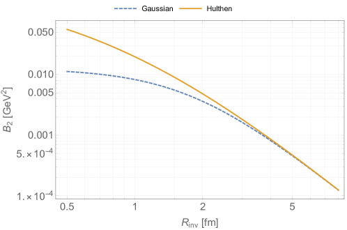
Figure 1: Deuteron coalescence factor $\mathcal{B}_{2}$, calculated in the isotropic (1D) Gaussian source model, showing the difference between the Gaussian and Hulthen wave function parameterisations.

To use the 3D source Eq. (41), the coalescence factor needs to be calculated numerically from Eq. (18) or (15).

III.3.2 Hypertriton wave function.

Hildenbrand & Hammer Hildenbrand and Hammer (2019) reported a three-body theoretical calculation of the ${\rm{}^{3}_{\Lambda}H}$ wave function. Green squares in the left panel of Fig. 2 show the projected $pn-\Lambda$ form factor obtained in that work. It is well reproduced by the two-body calculation of Congleton Congleton (1992), shown by solid red line, provided we adjust the $Q_{\Lambda}$ parameter of Congleton (1992) from $Q_{\Lambda}=1.17$ fm^-1 in the original paper to $Q_{\Lambda}=2.5$ fm^-1. For simplicity we therefore consider the effective $pn-\Lambda$ wave function from Congleton (1992), given in momentum space by

$$\hat{\phi}_{{\rm{}^{3}_{\Lambda}H}(\Lambda d)}({\bf q}) = A\frac{e^{-\frac{{\bf q}^{2}}{Q_{\Lambda}^{2}}}}{{\bf q}^{2}+\alpha_{\Lambda}^{2}}\;=\;\int d^{3}{\bf r}_{\Lambda}e^{-i{\bf r}_{\Lambda}{\bf q}_{\Lambda}}\phi_{{\rm{}^{3}_{\Lambda}H}(\Lambda d)}({\bf r}_{\Lambda})$$ (55)

where the normalisation constant $A$ is defined such that $\int d^{3}{\bf r}_{\Lambda}\left|\phi_{{\rm{}^{3}_{\Lambda}H}(\Lambda d)}({\bf r}_{\Lambda})\right|^{2}=\int\frac{d^{3}{\bf q}}{(2\pi)^{3}}\left|\hat{\phi}_{{\rm{}^{3}_{\Lambda}H}(\Lambda d)}({\bf q})\right|^{2}=1$. Using the $pn-\Lambda$ wave function of Congleton (1992), with $Q_{\Lambda}=2.5$ fm^-1 and $\alpha=0.068$ fm^-1, we can calculate the integrals in Eq. (34) or (30) numerically.

In the right panel of Fig. 2 we show numerical calculations from Hildenbrand and Hammer (2019), delimiting the uncertainty due to the ${}^{3}_{\Lambda}$H binding energy. We find that the lower (upper) range for the form factor is well fitted again by Congleton’s formula, with $Q_{\Lambda}=2.5$ fm^-1 and $\alpha=0.054$ (0.082) fm^-1, respectively.

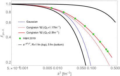
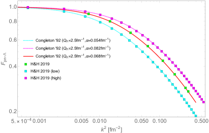
Figure 2: Hypertriton $pn-\Lambda$ form factor. Green squares show the result from the three-body calculation of Hildenbrand & Hammer Hildenbrand and Hammer (2019). Left: Dotted and solid red line shows the effective two-body calculation of Congleton Congleton (1992) for different values of their $Q_{\Lambda}$ parameter. Blue dashed line shows a Gaussian approximation with the same charge radius as found in Hildenbrand and Hammer (2019). For comparison, thick solid black lines show exponential factors with scale radius $R=1$ fm (top) and $5$ fm (bottom), respectively. Right: Cyan and magenta markers show a numerical calculation delimiting the uncertainty due to the ${}^{3}_{\Lambda}$H binding energy, as implemented in Hildenbrand and Hammer (2019).

Ref. Hildenbrand and Hammer (2019) also provided the effective form factor for the pn subsystem. Their numerical result is shown by black squares in Fig. 3. This form factor is reasonably well reproduced by a Gaussian of the form given by Eq. (48), with $b_{pn}=1.52$ fm (orange solid line). This can be compared with the low-${\bf k}^{2}$ expansion of the form factor, which would lead to $b_{pn}({\rm low-{\bf k}^{2}~{}fit})=1.73$ fm as noted in Sec. III.2. Given this discussion we can maintain the Gaussian ansatz of the pn factor in Eq. (48), setting $b_{pn}=1.52$ fm.

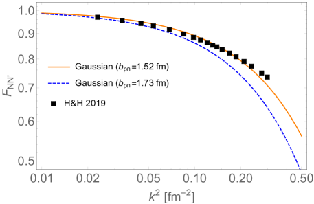
Figure 3: Hypertriton $pn$ form factor. Black squares show the result from the three-body calculation of Hildenbrand & Hammer Hildenbrand and Hammer (2019). Solid orange and dashed blue lines show a Gaussian approximation a-la Eq. (48) with $b_{pn}=1.52$ fm and $b_{pn}=1.73$ fm, respectively.

In Fig. 4 we plot $\mathcal{B}_{3\Lambda}$ vs $R_{\rm inv}$, showing the difference between the Gaussian (dashed grey) and the more realistic numerical (red) wave function parameterisations. Shaded band around the numerical result reflects the wave function uncertainty, as depicted in the right panel of Fig. 2.

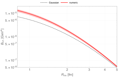
Figure 4: Hypertriton coalescence factor $\mathcal{B}_{3\Lambda}$, calculated in the isotropic (1D) Gaussian source model, showing the difference between the Gaussian (dashed grey) and the more realistic numerical (red) wave function parameterisations.

IV Comparison with data.

IV.1 Deuteron and ³He.

Fig. 5 shows the theoretical prediction for $\mathcal{B}_{2}$ (left) and $\mathcal{B}_{3}$ (right), calculated as function of the 1D HBT parameter $R_{\rm inv}$ using Eq. (III.3.1) (based on the Hulthen wave function) for D and Eq. (50) (Gaussian wave function) for ³He, with $R_{o}=R_{s}=R_{l}=R_{\rm inv}$. The calculation, shown by a grey shaded band, uses an estimate of the experimentally measured value of $\lambda_{2}$. To define the upper edge of the bands, we interpolate between $\lambda_{2}=\{1,0.7,0.7\}$ defined at $R_{\rm inv}=\{0.85,2.5,5\}$. To define the lower edge we interpolate between $\lambda_{2}=\{0.5,0.3,0.3\}$ defined at $R_{\rm inv}=\{0.85,2.5,5\}$. This range of $\lambda_{2}$ is estimated as follows. For large $R_{\rm inv}$ values we have a measurement of $\lambda_{2}$ in PbPb collisions Adam et al. (2015), obtained as the sum $\lambda_{2}\approx\lambda^{(pp)}+\lambda^{(p\Lambda)}$ in the notation of that paper. For small $R_{\rm inv}$ values, corresponding to pp collisions, we have no measurement of $\lambda_{2}$; Refs. Acharya et al. (2019a); Abelev et al. (2013a), which could in principle measure $\lambda_{2}$, effectively fixed $\lambda_{2}\to 1$ in their fit. As a next best solution we use $\lambda_{2}$ measured from kaon femtoscopy Abelev et al. (2013a). This is a potentially reasonable estimate because Ref. Adam et al. (2015) demonstrated HBT parameters that were the same, within measurement uncertainties, for kaon and proton final states at the same $m_{t}$. In addition to this attempt to estimate $\lambda_{2}$ from data we also show the result obtained fixing $\lambda_{2}=1$ (black solid line).

Based on our analysis in App. B we can expect that for the $p_{t}\lesssim 1.5$ GeV values, in which the cluster data in Fig. 5 are given, our use of the simplistic 1D source parameterisation should cause us to over-estimate a more accurate 3D prediction (not available to us, as the experiments reported 1D HBT fits only) by $\lesssim 20\%$ or so. We do not include this uncertainty in the plot. It adds up other sources of systematic uncertainty, expected to be roughly at a similar level (with unknown signs), due to the smoothness, equal-time, and factorisation approximations (the latter relevant for ³He only).

The comparison to experimental data is as follows. The red horizontal bands in Fig. 5 show experimental coalescence factor measurements for PbPb at (0-10%) (for $\mathcal{B}_{2}$) and (0-20%) (for $\mathcal{B}_{3}$) centrality classes Adam et al. (2016a). Each of the three red bands corresponds to a different bin in $m_{t}$, among the three bins shown in the HBT $R_{\rm inv}$ measurement Adam et al. (2015). The blue horizontal bands show the result for the (20-40%) (for $\mathcal{B}_{2}$) and (20-80%) (for $\mathcal{B}_{3}$) events, respectively, again from Adam et al. (2016a).

The green band shows the result for p-p collisions Acharya et al. (2018b).

For ³He we can also add a crudely estimated data point for pPb collisions. To do so, we combine the 1D HBT $R_{\rm inv}$ measurement of kaon femtoscopy reported in Acharya et al. (2019b) with the ³He measurement of Acharya et al. (2020b). To approximately match $m_{t}$ between the data sets, we use here the highest $k_{t}$ bin in Acharya et al. (2019b) and the lowest $p_{t}$ bin in Acharya et al. (2020b). We use the (0-20%) multiplicity class from Acharya et al. (2019b), joining together the (0-10%) and (10-20%) $\mathcal{B}_{3}$ data from Acharya et al. (2020b). The result is shown in purple in the right panel of Fig. 5.

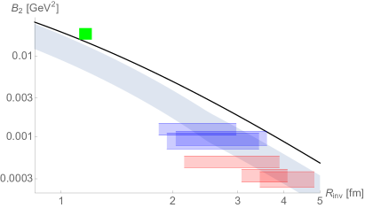
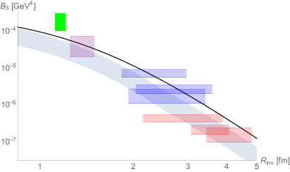
Figure 5: Summary of D and ³He data, reproduced from Ref. Blum and Takimoto (2019) with some improvements (see text). Left: $\mathcal{B}_{2}$ vs. $R_{\rm inv}$. Right: $\mathcal{B}_{3}$ vs. $R_{\rm inv}$.

As should be clear by now, a main uncertainty in the theory prediction shown in Fig. 5 is related to the determination of the chaoticity parameters $\lambda_{2}$ and $\lambda_{3}$. A measurement of $\lambda_{2}$ is missing for the pp and pPb systems, and we had to complete this information by using results from kaon femtoscopy. While the HBT results for kaons and protons come close to each other where they are available at the same value of $m_{t}$, it is clear that a proton HBT result is more suitable for the derivation of nuclear coalescence. For $\lambda_{3}$ we have no data, as such data would require three-proton femtoscopy. In Fig. 5 we bypassed this by assuming $\lambda_{3}=\lambda_{2}^{\frac{3}{2}}$. Addressing this issue experimentally would be challenging, and we do not know of a model-independent way to estimate the associated theory uncertainty. Assessing the uncertainty within specific HXS models, along the lines of App. B, may be warranted in future work.

Another obvious difficulty is due to the need to construct Fig. 5 patch-wise from data at different, often only partially overlapping, multiplicity class and $p_{t}$ or $m_{t}$ bins. A dedicated experimental analysis combining HBT and cluster yields would solve this problem.

Altogether, Fig. 5 shows that coalescence is roughly consistent with the D and ³He data for systems ranging from pp to pPb and PbPb at different regions of $p_{t}$ and at different multiplicity classes. This comparison spans a dynamical range of about a factor of 30 for $\mathcal{B}_{2}$ and a factor of $10^{3}$ for $\mathcal{B}_{3}$. While, as we discussed, there are theoretical and experimental uncertainties, there are no free parameters once HBT calibrates the computation. From this point of view, the usual claim to fame of the SHM Andronic et al. (2018), to describe the yields of nuclei across many orders of magnitude, is seen to be comparably well applicable to coalescence.

Having said that, it is worth highlighting that for pp collisions the experimental coalescence factors for both D and ³He are found to be higher than the coalescence prediction. Depending mainly on the poorly determined value of $\lambda_{2}$, but also on possible systematic uncertainties related to different event classes entering the HBT and cluster measurements, the discrepancy could be as much as a factor of 2 for D and a factor of 4 for ³He. We think that this situation is strong motivation for a joint experimental analysis of coalescence and HBT in small systems.

IV.2 Hypertriton.

Ref. Adam et al. (2016b) reported a measurement of ${}^{3}_{\Lambda}$H in PbPb collisions. After some gymnastics we extract the measured $\mathcal{B}_{3\Lambda}$ from the three $p_{t}$ bins in the left panel of their Fig. 7. For the bins $p_{t}\approx(0.66-1.34),\,(1.34-2),$ and $(2-2.34)$ GeV we find $\mathcal{B}_{3\Lambda}\approx(7.3-20)\times 10^{-8},\,(1-4.2)\times 10^{-7}$, and $(1.7-12)\times 10^{-5}$ GeV⁴, respectively. The multiplicity class is (0-10%). For HBT data, we have Ref. Adam et al. (2015) with $R_{\rm inv}$ and $\lambda_{2}$ measured in the same multiplicity class, but binned in $m_{t}$ rather than $p_{t}$ (see Figs. 7-8 in Adam et al. (2015)). We can match the first low $p_{t}$ bin of Adam et al. (2016b) into the $m_{t}$ range covered in Adam et al. (2015). We also consider the second $p_{t}$ bin of Adam et al. (2016b) that somewhat overshoots the coverage of the last $m_{t}$ bin in Adam et al. (2015). With some interpolation (and, for the second bin, extrapolation) of the results from Adam et al. (2015), we obtain the corresponding estimated ranges in $R_{\rm inv}$. The result is shown by markers in Fig. 6.

To plot the theory prediction, we need an estimate of $\lambda_{3\Lambda}$. On the left panel of Fig. 6 we set $\lambda_{3\Lambda}=\lambda_{2}^{\frac{3}{2}}$, with $\lambda_{2}$ taken in the range $(0.3-0.7)$, estimated from the data Adam et al. (2015). The theory prediction is shown by the red band, with the width of the band reflecting the allowed range in $\lambda_{2}$. In this exercise we use the numerical wave function of Sec. III.3.2. For reference, the result for $\lambda_{2}=1$ is shown by a black line. On the right panel we illustrate the wave function uncertainty, as well as the uncertainty (mentioned earlier in Sec. III.1) associated with determining $R_{\rm inv}$ from pp vs. p$\Lambda$ or $\Lambda\Lambda$ correlations. Setting $\lambda_{2}=0.5$ (in between 0.3 and 0.7), the result of varying the numerical wave function in the range corresponding to the right panel of Fig. 2 is shown by the red band. To implement the $R_{\rm inv}$ uncertainty, an orange band shows the effect of shifting the $R_{\rm inv}$ argument, entering the $\mathcal{B}_{3\Lambda}$ computation, by $\pm 20\%$ w.r.t. to the $R_{\rm inv}$ value on the x-axis. For comparison we also show the Gaussian wave function Eq. (51) in grey dashed. Black line for reference is same as on the left.

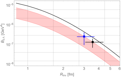
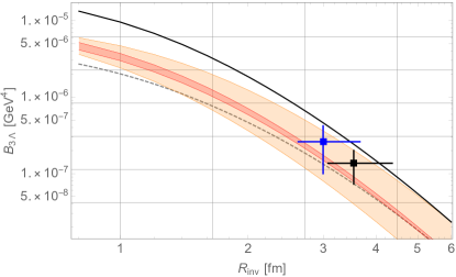
Figure 6: $\mathcal{B}_{3\Lambda}$ vs. the 1D HBT radius $R_{\rm inv}$. Left: The coalescence prediction for the numerical wave function of Sec. III.3.2, using $\lambda_{3}=\lambda_{2}^{\frac{3}{2}}$ taken from data (red band). The width of the band derives from the uncertainty on $\lambda_{2}$. For reference, the result for $\lambda_{2}=1$ is shown by solid black line. Right: Impact of wave function and $R_{\rm inv}$ uncertainties. Red band: numerical wave function uncertainty. Orange band: $R_{\rm inv}$ uncertainty (see text). Grey dashed: Gaussian wave function approximation. Black line is same as on the left.

Comparing between the left and right panels of Fig. 6 we can see that the estimated uncertainty due to the chaoticity parameter $\lambda_{3}$ (or $\lambda_{2}$) is larger than that due to the ${}^{3}_{\Lambda}$H wave function, again motivating an experimental effort to extract the chaoticity from data. We can also try to bypass some of this uncertainty as follows. If Nature is kind, and $\lambda_{3}\approx\lambda_{3\Lambda}$, then the uncertainty associated with $\lambda_{3\Lambda}$ may cancel in the ratio:

$$S_{3} = \frac{\mathcal{B}_{3\Lambda}}{\mathcal{B}_{3}}.$$ (56)

For the first $p_{t}$ bin of Adam et al. (2016b) we find $\mathcal{B}_{3}\approx(1.4-2.7)\times 10^{-7}$ GeV⁴, and for the second bin $\mathcal{B}_{3}\approx(3.3-6.9)\times 10^{-7}$ GeV⁴. We could, in principle, combine this directly with $\mathcal{B}_{3\Lambda}$ to extract the measured $S_{3}$. However, this would ignore the fact that some of the experimental uncertainty involved in deriving $\mathcal{B}_{3}$ and $\mathcal{B}_{3\Lambda}$ could cancel out in the ratio. Instead, we therefore adopt the following procedure. Taking the hypertriton spectrum from Adam et al. (2016b) (averaging the ${}^{3}_{\Lambda}$H and $\overline{{}^{3}_{\Lambda}{\rm H}}$ results), we divide by the ³He-spectrum from Adam et al. (2016a) and scale by the $\Lambda$/p ratio taken from Abelev et al. (2013b, c), evaluated in the corresponding $p_{t}$ interval. The result is shown by markers in Fig. 7.

The theoretical prediction for $S_{3}$, using the numerical ${}^{3}_{\Lambda}$H wave function of Sec. III.3.2, is shown by the red band in Fig. 7 with the band width determined by the wave function uncertainty. The effect of varying $R_{\rm inv}$ by $\pm 20\%$ is shown by the orange band. For comparison we also show the Gaussian approximation with a grey dashed line. The coalescence prediction is somewhat below the data, with tension at the $\sim 2\sigma$ level. It is clear from Fig. 7 that a more precise experimental measurement of $S_{3}$ in conjunction with HBT is a promising observable to exclude (or support) the framework. At small $R_{\rm inv}$, $S_{3}$ is predicted to be much below unity. Neither the ${}^{3}_{\Lambda}$H wave function uncertainty, nor the details of working with a 1D vs. 3D HBT source parameterisation are expected to enable, e.g., $S_{3}>0.2$ at $R_{\rm inv}\approx 1$ fm, characteristic for pp collisions.

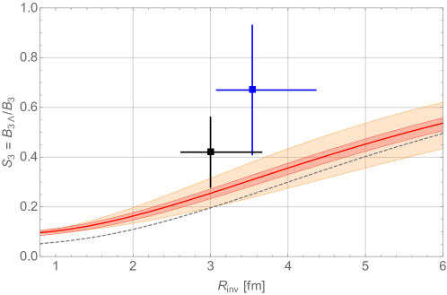
Figure 7: $S_{3}$ vs. $R_{\rm inv}$ predicted in the coalescence model compared with data.

V Discussion and summary.

The formation of nuclei by coalescence and femtoscopic [or Hanbury Brown-Twiss (HBT)] correlations between continuum proton pairs are two manifestations of final state interactions (FSI) that “dress” an underlying high-excitation state (HXS) produced in hadronic collisions. In Sec. II, starting from a relativistic quantum field theoretic (QFT) computation, we recalled how the effective quantum mechanical (QM) description of the dynamics of pairs that are nonrelativistic in the pair rest frame (PRF) gives rise to the usual HBT formalism, with which a two-particle source, characterising the HXS, can be measured. The same two-particle source enters the coalescence formula for deuteron formation. Much of our analysis was based on the formalism reviewed by Lednicky Lednicky (2009); our contribution was to reduce this formalism to observationally accessible language in the context of nuclear clusters. In both cases – HBT and coalescence – effective QM holds for ${\bf q^{2}\ll m^{2}}$, where ${\bf q}$ is the PRF momentum difference and $m$ is the nucleon mass; and up to corrections of order $\sim 0.2\frac{\rm 1fm}{\bf x}$, where ${\bf x}$ is the average PRF characteristic distance between the nucleons in the HXS. Although it should not be trusted beyond $\mathcal{O}(10\%)$ accuracy, the QM limit is useful for deriving simple physically-transparent formulae and should be sufficient for ruling out (or supporting) coalescence as the origin of nuclei in hadronic collisions. In principle, while we did not pursue this route, the QM approximation can be avoided if one works directly with the relativistic FSI Bethe-Salpeter amplitudes.

Coalescence after kinetic freeze out must occur at some level in hadronic collisions, but this does not mean that it is necessarily the dominant origin of clusters. The key assumption made by the coalescence model is that the long-range action of FSI can be factored out of an underlying short-range HXS dynamics. The level of accuracy of this factorisation is not obvious. To some extent, the apparent success of HBT analyses Adam et al. (2015); Acharya et al. (2019a, 2020a) in reconstructing a fit of the two-nucleon source, using sophisticated physical FSI calculations, supports the coalescence framework. But we feel that this is not yet fully convincing: while the HBT analyses Adam et al. (2015); Acharya et al. (2019a, 2020a) reported measurements of the two-nucleon source with a stated precision of $\mathcal{O}(10\%)$, they did so using a naive 1D Gaussian source fit. However, the true underlying source is not expected to be 1D; in fact, at least for mean lab frame momentum ${\bf p}\gtrsim m$, it must be anisotropic at the $\mathcal{O}(1)$ level – as seen in the PRF – due to Lorentz contraction. We can add to this the chaoticity parameter $\lambda_{2}$ (denoted just $\lambda$ in most of the literature), which was found to be significantly smaller than 1 in Adam et al. (2015), but was held fixed to 1 in the fit of Acharya et al. (2019a, 2020a). Altogether, it is clear that higher statistics HBT analyses have an important future role to play Citron et al. (2019) in establishing to what extent true physical HXS information is revealed in femtoscopy. Our work highlights the importance of this question also to the origin of clusters.

Keeping the caveats above in mind, the main point of our work is to establish the coalescence/femtoscopy framework as a means to test coalescence by grounding the coalescence predictions with HBT information. The coalescence–correlations relation between HBT and deuteron formation, summarised by Eqs. (14,15) [or equivalently Eqs. (16,18) in momentum space], was derived first in Blum and Takimoto (2019) in the QM limit. The relation is very general and model-independent. As shown in Blum and Takimoto (2019), it is consistent with the early model-dependent derivation of Scheibl and Heinz (1999) (the latter, however, specialised to a particular model of hydrodynamical flow and was limited to small $p_{t}$). It is also consistent with the body of work by Mrowczynski Mrowczynski (1987, 1990, 1992, 1993, 1995); Maj and Mrowczynski (2005); Mrowczynski (2017).

The connection of HBT with deuteron formation does not rely on density matrix factorisation. To derive formulae for three-body clusters, though, factorisation is needed. Assuming factorisation we derived the formulae for ${}^{3}_{\Lambda}$H and ³He, summarised in Eqs. (30,31) [or Eqs. (34,35) in momentum space]. As an aside, we note that the derivation does not leave room for the confusion between “pn$\Lambda$ channel” and “D$\Lambda$ channel” advocated in Zhang and Ko (2018); Sun et al. (2019) for ${}^{3}_{\Lambda}$H. Three-body coalescence comes from three-body FSI and is captured by a single formula, involving the three-body nucleus wave function.

In Sec. III we combined formulae for the two-nucleon source, constrained by experimental HBT fits, with nuclear wave functions to obtain expressions for coalescence factors that can be compared to data. Exploring different forms for the wave function of ${}^{3}_{\Lambda}$H, we showed that although a full numerical representation of the wave function deviates significantly from a Gaussian, the numerical impact on the coalescence factor is modest, about a factor of two (with the more realistic numerical wave function predicting a higher coalescence factor). Our calculations allow for different scales in the wave functions of three-body states. This is particularly important for ${}^{3}_{\Lambda}$H where the pn-$\Lambda$ factor is significantly more extended than the effective pn factor. Some earlier implementations Bellini and Kalweit (2019) of the coalescence–correlations relation for ${}^{3}_{\Lambda}$H did not account for this fact.

Our calculations also account for the anisotropic shape of the two- and three-nucleon source describing the HXS. As we illustrate in App. B, the two-particle source is expected to be truly anisotropic in nature, especially at large $p_{t}$.

In Sec. IV we compared our theoretical predictions to data. Fig. 5 shows that coalescence, calibrated by HBT, is consistent at the $\mathcal{O}(1)$ level with the $p_{t}$-differential yields of D and ³He for systems ranging from pp, pPb to PbPb and across different centralities. This comparison spans a dynamical range of $\sim 30$ for $\mathcal{B}_{2}$ and $\sim 10^{3}$ for $\mathcal{B}_{3}$. Some tension, at the $\sim 2\sigma$ level or so, is seen for pp in both of the D and ³He yields. This situation gives strong motivation for a dedicated experimental analysis, studying HBT and cluster yields side by side in the same data set under the same kinematic conventions and cuts. On the HBT side, we urge the experiments to report HBT measurements allowing the chaoticity parameter $\lambda_{2}$ to float in the fit. In addition, as much as statistics permits, measurements of the 3D source (in the out-side-long parameterisation) would be preferred over 1D measurements of $R_{\rm inv}$. Such combined experimental analysis could zoom in on the coalescence–correlations prediction beyond the $\mathcal{O}(1)$ level by which it can currently be tested. This could, in principle, sharpen tensions with D and/or ³He data where they are currently difficult to establish conclusively.

Hypertriton ${}^{3}_{\Lambda}$H is known as a sensitive test of coalescence because of its large size, suggesting that the QM factor discriminating coalescence from the statistical hadronisation model (SHM) should be small and discernible. Our calculation, depicted in Fig. 6, shows that the current measurements of $\mathcal{B}_{3\Lambda}$ in PbPb collisions are consistent with the coalescence prediction. The observable $S_{3}=\mathcal{B}_{3\Lambda}/\mathcal{B}_{3}$ may be more robust than $\mathcal{B}_{3\Lambda}$, because some experimental and theoretical uncertainties may cancel in the ratio. We compare our calculation of $S_{3}$ with the data in Fig. 7, finding some tension: the $S_{3}$ data tends to be somewhat higher than coalescence predicts. This discrepancy is not (yet) very significant, around $2\sigma$. A higher statistics measurement, and measurements in small systems like pp, pPb, or low multiplicity PbPb collisions – in short, systems with small HBT radius – would provide a critical test of coalescence.

Appendix A Corrections to the Gaussian source approximation.

The Gaussian source considered in Sec. III.1 cannot be exact. It is therefore important to estimate the uncertainty in the coalescence calculation, that comes about if this approximation is used. In this section we consider mechanisms that violate the Gaussian source approximation and estimate their quantitative impact.

A.1 Feed-down from weak decays and source chaoticity.

In comparing theory to data one should account for the effect of feed-down from weak decay, where a particle that is emitted from the HXS as $\Lambda$ or $\Sigma$ decays into a proton in the detector (see Wiedemann and Heinz (1997) for a parallel discussion for pions). The decay vertex is displaced by $\mathcal{O}(1~{}{\rm cm})$ from the HXS, which means that the FSI relevant for two-particle correlation are those involving $\Lambda$ or $\Sigma$. Ref. Acharya et al. (2020a) estimated that a fraction $\alpha_{p}\approx 0.82$ of detected protons in their analysis originate from a genuine emitted proton, while a fraction $\alpha_{\Lambda}\approx 0.12$ and a fraction $\alpha_{\Sigma}\approx 0.06$ of detected protons originate from an emitted $\Lambda$ or $\Sigma$, respectively. Neglecting particle misidentification (which add up to about 1% in Acharya et al. (2020a)) we have $\alpha_{p}\approx 1-\alpha_{\Lambda}-\alpha_{\Sigma}$. Thus, if HBT correlations are ignored, a fraction $\lambda^{(pp)}\approx(1-\alpha_{\Lambda}-\alpha_{\Sigma})^{2}\approx 0.7$ of detected pp pairs come from genuine emitted pp, while, for example, a fraction $\lambda^{(p\Lambda)}\approx 2\alpha_{\Lambda}(1-\alpha_{\Lambda}-\alpha_{\Sigma})\approx 0.2$ of detected pp pairs come from an emitted p$\Lambda$ pair, etc.

In constructing the observable two-proton correlation, Refs. Adam et al. (2015); Acharya et al. (2019a, 2020a) divided the measured proton pair spectrum by the spectrum of pairs from uncorrelated mixed events, without feed-down subtraction. Then, in fitting a model of the correlation to the data, the correlation function was split into a part coming from genuine emitted pp pairs and parts coming from emitted p$\Lambda,\,\Lambda\Lambda,\,p\Sigma$ and $\Sigma\Sigma$ pairs, using the relevant FSI for each part:

$$C^{\rm model}({\bf p,q}) = 1+\sum_{i={\rm pp,p\Lambda,...}}\lambda^{(i)}\left[C^{(i)}({\bf p,q})-1\right],$$ (57)

with the channel-specific weights and correlation functions

$$C^{(i)}({\bf p,q}) = \sum_{s}w_{s}\int d^{3}{\bf r}\,\mathcal{S}_{2}^{(i)}({\bf r})\left|\phi^{(i)}_{s,q}({\bf r})\right|^{2}.$$ (58)

Here, for example, for $i=p\Lambda$ the wave function at spin channel $s$ is given by $\phi^{(p\Lambda)}_{s,q}({\bf r})$, etc. In Ref. Acharya et al. (2020a), the nucleon source functions $\mathcal{S}_{2}^{(i)}({\bf r})$ were modelled differently for different $i$, to account for strong resonances that have a different characteristic decay range for p and $\Lambda$ daughters. In contrast, Refs. Adam et al. (2015); Acharya et al. (2019a) assumed a common nucleon source $\mathcal{S}_{2}^{(i)}=\mathcal{S}_{2}$.

As long as the $\lambda^{(i)}$ parameters are correctly calibrated to account for weak decays, a quick check verifies that the correlation functions $C^{(i)}$ in Eq. (58) do indeed match with the theoretical definition of the same objects as derived in Sec. II.1. Refs. Acharya et al. (2019a, 2020a) assumed that this was the case and fixed the numerical values of the $\lambda^{(i)}$ according to the experimentally determined single proton purity. In contrast, Ref. Adam et al. (2015) did not fix the value of $\lambda^{(pp)}$ and $\lambda^{(p\Lambda)}$, but rather considered these parameters as part of the experimental fit. Interestingly, the fit resulted in $\lambda\equiv\lambda^{(pp)}+\lambda^{(p\Lambda)}\approx 0.3-0.7$, significantly less than unity.

From the theoretical point of view, the approach of Adam et al. (2015) is beneficial over that of Acharya et al. (2019a, 2020a). The reason has to do with the modelling of the source function $\mathcal{S}_{2}({\bf r})$ Heinz and Jacak (1999); Blum and Takimoto (2019). Refs. Adam et al. (2015); Acharya et al. (2019a, 2020a) assumed in their fit the 1D Gaussian form Eq. (36). This source function integrates to unity, $\int d^{3}{\bf r}\,\mathcal{S}_{2}({\bf r})=1$, corresponding to $\mathcal{C}_{2}({\bf q}=0)=1$. However, there is no a-priori reason to assume that the true $\mathcal{C}_{2}$ (or $\mathcal{S}_{2}$) satisfy this normalisation exactly. In fact, observing a departure from this normalisation in the data could hint, for example, at a violation of the factorisation assumption of Sec. II.2. In addition, it is well known that if the experimental fit assumes a Gaussian form for $\mathcal{C}_{2}({\bf q})$, but the true $\mathcal{C}_{2}({\bf q})$ is non-Gaussian, then adding an intercept parameter $\lambda_{2}$ to the fit, as in Eq. (41), can absorb some of the difference.

We can thus interpret the $\lambda$ measurement of Adam et al. (2015) as a measurement of the parameter $\lambda_{2}$, via $\lambda_{2}\approx\lambda$. In contrast, the analysis of Refs. Acharya et al. (2019a, 2020a) effectively forced $\lambda_{2}\to 1$ in the fit procedure.

Considering now the coalescence factor, a direct comparison to the HBT analysis is possible if the single proton spectrum used in the experimental definition of $\mathcal{B}_{A}$ (e.g. Eq. (10)) is obtained subtracting the weak decay feed-down contributions. With this the coalescence–correlation relation of Eq. (15) or Eq. (18) applies as is. For $\mathcal{B}_{3,3\Lambda}$, a fully data-driven analysis would require an experimental measurement of $\mathcal{C}_{3}$. In the absence of that, we can roughly estimate that for $\lambda_{2}\neq 1$ the Gaussian source expressions for $\mathcal{B}_{3,3\Lambda}$ should be modified by $\mathcal{B}_{3,3\Lambda}\to\lambda_{2}^{\frac{3}{2}}\mathcal{B}_{3,3\Lambda}$ Blum and Takimoto (2019).

Unrelated to weak decays, a correction to the expressions of Sec. III arises from the fact that Ref. Acharya et al. (2020a) actually found different fit results for the sources $\mathcal{S}_{2}({\bf r})$ deduced from pp and p$\Lambda$ pairs. One physically motivated reason for the difference stems from the different decay range of the strong resonances, that feed into p and $\Lambda$ states in the HXS. The same effect also predicts a non-Gaussian form for $\mathcal{S}_{2}({\bf r})$ (and $\mathcal{C}_{2}({\bf q})$), as we discuss next.

A.2 Strong resonance decays.

Even if the underlying emission function was an exact Gaussian, the decay of strong resonances with lifetimes of the order of a few fm would distort the effective source. Ref. Acharya et al. (2020a) studied this problem for pp and p$\Lambda$ correlations in pp collisions. An isotropic source model including strong resonance decay, which was found in Acharya et al. (2020a) to give an adequate fit to the correlation data, is reproduced here in the left panel of Fig. 8. The full (non Gaussian) source is shown by circles, compared with the Gaussian source in dotted lines. Strong resonances lead to a non Gaussian tail of $\mathcal{S}_{2}({\bf r})$.

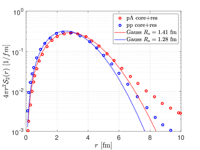
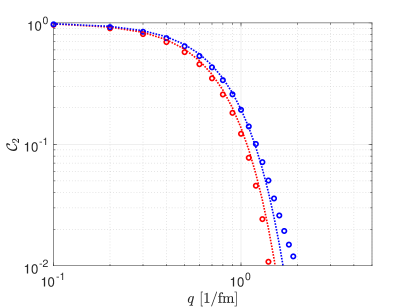
Figure 8: Left: The source $\mathcal{S}_{2}(\bf r)$, reproduced from the experimental fit result of Fig. 4 in Ref. Acharya et al. (2020a). Right: $\mathcal{C}_{2}$, the Fourier transform of the sources on the left.

In the right panel of Fig. 8 we show the $\mathcal{C}_{2}({\bf q})$ curves corresponding to the $\mathcal{S}_{2}({\bf r})$ curves on the left.

Quantitatively, despite the strong resonance contribution, the Gaussian approximation can be seen to give a rather accurate description of the source: the difference between the full non Gaussian $\mathcal{C}_{2}$ and the Gaussian approximation is smaller than $\sim 10\%$ throughout the range where $\mathcal{C}_{2}>0.1$. While Ref. Acharya et al. (2020a) dealt with pp initial state, we might expect that in larger systems like PbPb the relative impact of strong resonance decay could be even less significant.

We emphasise that Ref. Acharya et al. (2020a), which provided the example for our discussion, assumed an underlying Gaussian source which they then deformed by strong resonances. What we learn from this exercise, then, is that if the underlying “genuine” emission function is Gaussian, then the effective two-particle source after strong decays is also consistent with Gaussian to 10% accuracy, in the range of ${\bf r}$ (or, in momentum space, ${\bf q}$) that is relevant for coalescence. We stress, however, that while the assumed 1D Gaussian source of Acharya et al. (2020a) was experimentally consistent with HBT data, there is no guarantee that the true physical source is Gaussian. In App. B we recall theoretical reasons to expect otherwise.

Appendix B Deviations from an isotropic Gaussian source in the phenomenological blast wave model.

Relativistic expansion of the HXS “fire ball” is expected to proceed differently along and transverse to the beam line. This unisotropic flow predicts that the source $\mathcal{S}_{2}({\bf r})$ should depend on the direction of ${\bf r}$ w.r.t. the beam line and also w.r.t. the pair mean momentum vector ${\bf p}$. Even if the nucleon source was somehow isotropic in the lab frame, it would not be seen as isotropic in the PRF for ${\bf p}\neq 0$, due to Lorentz contraction. These effects were not modelled in the experimental analyses of Refs. Adam et al. (2015); Acharya et al. (2019a, 2020a), that performed fits to the 1D source Eqs. (39). Here we consider these effects from the point of view of the phenomenological blast wave model (BWM). Our goal is not to argue either in favour or against the validity of the model, but simply to gain some feeling for the possible systematic error associated with adopting the 1D Gaussian source approximation, if that is applied to coalescence calculations via the coalescence–correlation relation.

To recall the BWM, we take the beam line to be along the $\hat{z}$ axis. The space-time coordinates are chosen as $\tau=\sqrt{t^{2}-z^{2}}$, $\rho=\sqrt{x^{2}+y^{2}}$, $\eta={\rm arctanh}(z/t)$, and the azimuthal angle $\phi$. The position 4-vector is then $R^{\mu}=\left(\tau\cosh\eta,\rho\cos\phi,\rho\sin\phi,\tau\sinh\eta\right)$ and $d^{4}R=d\tau\tau\,d\rho\rho\,d\eta\,d\phi$. The 4-momentum vector of a particle emitted at rapidity $Y$, azimuthal angle $\Phi$, and transverse momentum $p_{t}$, is $p^{\mu}=\left(m_{t}\cosh Y,p_{t}\cos\Phi,p_{t}\sinh\Phi,m_{t}\sinh Y\right)$, with $m_{t}=\sqrt{m^{2}+p_{t}^{2}}$. The single-particle emission function is parameterized using 6 parameters, $\tau_{0},\Delta\tau,R_{0},\beta_{S},n,T$ (we neglect chemical potentials), as follows ($\theta(x)$ is the Heaviside step function):

$$\tilde{S}_{p}(R) = \sqrt{\frac{2}{\pi}}\frac{m_{t}}{m}\cosh\left(\eta-Y\right)J(\tau)\theta\left(R_{0}-\rho\right)e^{-\frac{pu}{T}},$$ (59)

$$u^{\mu}(R) = \left(\cosh\eta\cosh\eta_{t},\sinh\eta_{t}\cos\phi,\sinh\eta_{t}\sin\phi,\sinh\eta\cosh\eta_{t}\right),$$ (60)

$$\eta_{t}(\rho) = {\rm tanh}^{-1}\left(\frac{\rho^{n}}{R_{0}^{n}}\,\beta_{S}\right),$$ (61)

$$J(\tau) = \frac{1}{\sqrt{2\pi}\Delta\tau}e^{-\frac{(\tau-\tau_{0})^{2}}{2\Delta\tau^{2}}}.$$ (62)

With these definitions we can evaluate $\mathcal{C}_{2}(p,{\bf q})$ numerically via Eq. (25). In doing so, recall that we require $q=(0,{\bf q})$ specified in the PRF, while the emission function $\tilde{S}_{p}(x)$ depends on space-time coordinates in the lab frame. Defining $b=p/m$, we can write $q^{\prime}$ in the lab frame as $q^{\prime 0}={\bf bq},\;\;{\bf q}^{\prime}={\bf q}+\frac{\bf bq}{1+b^{0}}{\bf b}$ Scheibl and Heinz (1999). For simplicity, in the examples below we choose $p=(m_{t},p_{t},0,0)$. With this choice $pu=m_{t}\cosh\eta\cosh\eta_{t}-p_{t}\sinh\eta_{t}\cos\phi$ and using the $q_{l},q_{o},q_{s}$ decomposition we have $qx=\frac{p_{t}}{m}q_{o}\tau\cosh\eta-\frac{m_{t}}{m}q_{o}\rho\cos\phi-q_{s}\rho\sin\phi-q_{l}\tau\sinh\eta$. We consider separately the cases ${\bf q}=(q_{o},0,0)$, ${\bf q}=(0,q_{s},0)$, and ${\bf q}=(0,0,q_{l})$.

In Fig. 9 we plot $\mathcal{C}_{2}(p,{\bf q})$, projected onto the out, side, and long directions (solid blue, orange, and green, respectively). Independent Gaussian fits to each projection are shown by dotted lines. Black dashed line shows the 1D Gaussian source computed with $R_{\rm inv}=\left(R_{o}R_{s}R_{l}\right)^{\frac{1}{3}}$. For definiteness we take $T=100$ MeV, $n=1$, $\beta_{s}=0.5$ and $\tau_{0}=7$ fm, $\Delta\tau=1.5$ fm, $R_{0}=7$ fm, chosen to roughly represent PbPb collisions Adam et al. (2016a). Note that the phenomenological BWM is based on classical intuition and satisfies by construction – effectively – the density matrix factorisation assumption. Thus the chaoticity parameters $\lambda_{2}=\lambda_{3}=1$ in this computation, and we are guaranteed that $\mathcal{C}_{2}(p,{\bf 0})=1$.

The source depicted in Fig. 9 was chosen to resemble PbPb collisions. From the fits in the plot, the radii of homogeniety for this source at $p_{t}=0$, for example, are $R_{o}=R_{s}\approx 3.2$ fm, $R_{l}\approx 2.5$ fm, extended compared to the deuteron RMS radius $r_{rms}=\sqrt{3/8}b_{d}\approx 2.1$ fm. To see the size of the effect for smaller systems, e.g. pp collisions, we recalculate $\mathcal{C}_{2}$ for different values of $R_{0}=\tau_{0}=2$ fm, leading to $R_{o}=R_{s}\approx 0.9$ fm, $R_{l}\approx 1$ fm at $p_{t}=0$. (The other BWM parameters are unchanged.) The results are shown in Fig. 10.

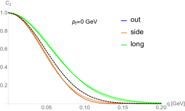
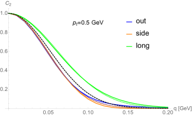
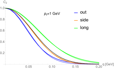
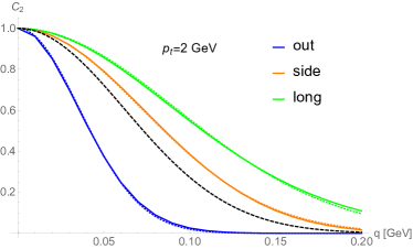
Figure 9: The two-particle source $\mathcal{C}_{2}(p,{\bf q})$ calculated in the blast wave model and projected onto the out, side, long directions. Solid lines show the numerical result, while dotted lines show independent Gaussian fits to each projection. Black dashed line shows the 1D Gaussian source with $R_{\rm inv}=\left(R_{o}R_{s}R_{l}\right)^{\frac{1}{3}}$. The BWM parameters are chosen to mimic PbPb collisions at the LHC (see text). Top left, top right, bottom left, bottom right: $p_{t}=0,0.5,1,2$ GeV.

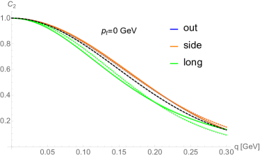
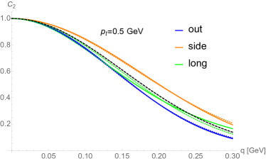
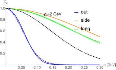
Figure 10: Same as Fig. 10, with BWM model parameters chosen to mimic pp collisions at the LHC.

Figs. 9-10 demonstrate how unisotropic flow leads to an unisotropic source. Notably, the width along the out direction shows Lorentz contraction in the PRF at $p_{t}>0$. This perspective calls into question the attempt in Acharya et al. (2020a) to fit the details of $\mathcal{S}_{2}({\bf r})$ to $\mathcal{O}(10\%)$ precision, based on the 1D isotropic Gaussian model.

Our main interest is to check to what extent the deviation from 1D Gaussian source affects the coalescence calculation. Again from Figs. 9-10 (as well as from the discussion in Sec. A.2), we expect that a 3D Gaussian approximation may do a reasonably accurate job describing $\mathcal{C}_{2}$; thus we will use the 3D Gaussian parameterisation as a standard for comparison. For a rough estimate of the error, incurred by using the 1D fit of Eq. (39) to describe a 3D source, we calculate $R_{o},R_{s},R_{l}$ in the BWM and define

$$R_{\rm inv} = \left(R_{o}R_{s}R_{l}\right)^{\frac{1}{3}}.$$ (63)

We can now compare the results of using Eq. (49) with $R_{o}=R_{s}=R_{l}\to R_{\rm inv}$, to the results of the original Eq. (49):

$$\frac{\mathcal{B}_{2}^{1D}}{\mathcal{B}_{2}^{3D}} \sim \sqrt{\frac{\left(b_{d}^{2}+4R_{l}^{2}\right)\left(b_{d}^{2}+4R_{o}^{2}\right)\left(b_{d}^{2}+4R_{s}^{2}\right)}{\left(b_{d}^{2}+4R_{\rm inv}^{2}\right)^{3}}}.$$ (64)

Note that in both limits $b_{d}\to 0$ and $b_{d}\to\infty$ this correction factor is equal to 1. The results are summarised in Tab. 1.

We give a rough estimate of the correction to $\mathcal{B}_{3\Lambda}$ in a similar way:

$$\frac{\mathcal{B}_{3\Lambda}^{1D}}{\mathcal{B}_{3\Lambda}^{3D}} \sim \sqrt{\frac{\left(b_{pn}^{2}+2R_{l}^{2}\right)\left(b_{\Lambda}^{2}+2R_{l}^{2}\right)\left(b_{pn}^{2}+2R_{o}^{2}\right)\left(b_{\Lambda}^{2}+2R_{o}^{2}\right)\left(b_{pn}^{2}+2R_{s}^{2}\right)\left(b_{\Lambda}^{2}+2R_{s}^{2}\right)}{\left(b_{pn}^{2}+2R_{\rm inv}^{2}\right)^{3}\left(b_{\Lambda}^{2}+2R{\rm inv}^{2}\right)^{3}}}.$$ (65)

The calculation for $\mathcal{B}_{3}$ is the same up to $b_{pn}\to b_{\Lambda}\to b_{\rm{}^{3}He}$. The results are also summarised in Tab. 1.

Table 1: The corrections of Eqs. (64-65), comparing between the coalescence factor obtained from a 1D and a 3D Gaussian fit to $\mathcal{C}_{2}$ computed in the BWM. We round the result to two significant digits.

$p_{t}$	$m_{t}$	$\mathcal{B}_{2}^{1D}/\mathcal{B}_{2}^{3D}$	$\mathcal{B}_{2}^{1D}/\mathcal{B}_{2}^{3D}$	$\mathcal{B}_{3}^{1D}/\mathcal{B}_{3}^{3D}$	$\mathcal{B}_{3}^{1D}/\mathcal{B}_{3}^{3D}$	$\mathcal{B}_{3\Lambda}^{1D}/\mathcal{B}_{3\Lambda}^{3D}$	$\mathcal{B}_{3\Lambda}^{1D}/\mathcal{B}_{3\Lambda}^{3D}$
${\rm[GeV]}$	${\rm[GeV]}$	PbPb	pp	PbPb	pp	PbPb	pp
0	0.94	1	1	1	1	1	1
0.5	1.07	1	1	1	1	1	1
1	1.37	1	1.1	1	1.1	1	1.1
2	2.2	1.1	1.3	1.2	1.9	1.2	1.5

We have also done a numerical calculation of the ratio $\mathcal{B}_{2}^{1D}/\mathcal{B}_{2}^{3D}$ using the Hulthen D wave function. In this exercise we calculated $\mathcal{B}_{2}^{3D}$ from Eq. (15), comparing that with the result of Eq. (III.3.1). The results we find for PbPb and pp and for all values of $p_{t}$ are numerically very close to those found in Tab. 1 using the Gaussian wave function.

The conclusion from Tab. 1 is that the 1D Gaussian parameterisation tends to slightly over-estimate the coalescence factor, in comparison to the more accurate 3D parameterisation. The effect is more pronounced in small systems than in PbPb, and increases with increasing $p_{t}$. Using the 1D $R_{\rm inv}$ parameterisation results with $\mathcal{O}(10\%)$ error at $p_{t}\sim 1$ GeV, rising to as much as a factor of 2 for ³He at $p_{t}=2$ GeV in pp collisions. It should be stressed that these conclusions are drawn from simple, model-dependent calculations in the BWM, and should only be taken as crude estimates of the theoretical uncertainty in the coalescence calculation.

References

- Csernai and Kapusta (1986) L. P. Csernai and J. I. Kapusta, Phys. Rept. 131, 223 (1986).
- Andronic et al. (2011) A. Andronic, P. Braun-Munzinger, J. Stachel, and H. Stocker, Phys. Lett. B 697, 203 (2011), eprint 1010.2995.
- Cleymans et al. (2011) J. Cleymans, S. Kabana, I. Kraus, H. Oeschler, K. Redlich, and N. Sharma, Phys. Rev. C 84, 054916 (2011), eprint 1105.3719.
- Andronic et al. (2018) A. Andronic, P. Braun-Munzinger, K. Redlich, and J. Stachel, Nature 561, 321 (2018), eprint 1710.09425.
- Vovchenko et al. (2018) V. Vovchenko, B. D nigus, and H. Stoecker, Phys. Lett. B 785, 171 (2018), eprint 1808.05245.
- Vovchenko et al. (2019) V. Vovchenko, B. D nigus, and H. Stoecker, Phys. Rev. C 100, 054906 (2019), eprint 1906.03145.
- Acharya et al. (2018a) S. Acharya et al. (ALICE), Nucl. Phys. A 971, 1 (2018a), eprint 1710.07531.
- Shuryak and Torres-Rincon (2019) E. Shuryak and J. M. Torres-Rincon, Phys. Rev. C 100, 024903 (2019), eprint 1805.04444.
- Shuryak and Torres-Rincon (2020) E. Shuryak and J. M. Torres-Rincon, Phys. Rev. C 101, 034914 (2020), eprint 1910.08119.
- Juric et al. (1973) M. Juric et al., Nucl. Phys. B 52, 1 (1973).
- Lisa et al. (2005) M. A. Lisa, S. Pratt, R. Soltz, and U. Wiedemann, Ann. Rev. Nucl. Part. Sci. 55, 357 (2005), eprint nucl-ex/0505014.
- Heinz and Jacak (1999) U. W. Heinz and B. V. Jacak, Ann. Rev. Nucl. Part. Sci. 49, 529 (1999), eprint nucl-th/9902020.
- Oliinychenko et al. (2019) D. Oliinychenko, L.-G. Pang, H. Elfner, and V. Koch, Phys. Rev. C 99, 044907 (2019), eprint 1809.03071.
- Lednicky (2007) R. Lednicky, Braz. J. Phys. 37, 939 (2007), eprint nucl-th/0702063.
- Scheibl and Heinz (1999) R. Scheibl and U. W. Heinz, Phys. Rev. C59, 1585 (1999), eprint nucl-th/9809092.
- Lednicky and Lyuboshits (1982) R. Lednicky and V. L. Lyuboshits, Sov. J. Nucl. Phys. 35, 770 (1982), [Yad. Fiz.35,1316(1981)].
- Akkelin et al. (2002) S. Akkelin, R. Lednicky, and Y. Sinyukov, Phys. Rev. C 65, 064904 (2002), eprint nucl-th/0107015.
- Lednicky (2009) R. Lednicky, Phys. Part. Nucl. 40, 307 (2009), eprint nucl-th/0501065.
- Blum and Takimoto (2019) K. Blum and M. Takimoto, Phys. Rev. C 99, 044913 (2019), eprint 1901.07088.
- Hildenbrand and Hammer (2019) F. Hildenbrand and H. W. Hammer, Phys. Rev. C100, 034002 (2019), eprint 1904.05818.
- Zhang and Ko (2018) Z. Zhang and C. M. Ko, Phys. Lett. B 780, 191 (2018).
- Sun et al. (2019) K.-J. Sun, C. M. Ko, and B. D nigus, Phys. Lett. B 792, 132 (2019), eprint 1812.05175.
- Bellini and Kalweit (2019) F. Bellini and A. P. Kalweit, Phys. Rev. C 99, 054905 (2019), eprint 1807.05894.
- Koonin (1977) S. E. Koonin, Phys. Lett. 70B, 43 (1977).
- Bond et al. (1977) R. Bond, P. Johansen, S. Koonin, and S. Garpman, Phys. Lett. B 71, 43 (1977).
- Sato and Yazaki (1981) H. Sato and K. Yazaki, Phys. Lett. 98B, 153 (1981).
- Mrowczynski (1987) S. Mrowczynski, J. Phys. G13, 1089 (1987).
- Mrowczynski (1990) S. Mrowczynski, Phys. Lett. B248, 459 (1990).
- Mrowczynski (1992) S. Mrowczynski, Phys. Lett. B277, 43 (1992).
- Mrowczynski (1993) S. Mrowczynski, Phys. Lett. B308, 216 (1993).
- Mrowczynski (1995) S. Mrowczynski, Phys. Lett. B345, 393 (1995), eprint hep-ph/9502215.
- Maj and Mrowczynski (2005) R. Maj and S. Mrowczynski, Phys. Rev. C71, 044905 (2005), eprint nucl-th/0409061.
- Mrowczynski (2017) S. Mrowczynski, Acta Phys. Polon. B48, 707 (2017), eprint 1607.02267.
- Blum et al. (2017) K. Blum, K. C. Y. Ng, R. Sato, and M. Takimoto, Phys. Rev. D96, 103021 (2017), eprint 1704.05431.
- Pratt and Tsang (1987) S. Pratt and M. Tsang, Phys. Rev. C 36, 2390 (1987).
- Martin et al. (1996) L. Martin, C. Gelbke, B. Erazmus, and R. Lednicky, Nucl. Phys. A 604, 69 (1996).
- Schweber et al. (1955) S. S. Schweber, H. A. Bethe, and F. de Hoffmann (1955).
- Pratt (1997) S. Pratt, Phys. Rev. C 56, 1095 (1997).
- Landau and Lifshits (1991) L. D. Landau and E. Lifshits, Quantum Mechanics: Non-Relativistic Theory, vol. v.3 of Course of Theoretical Physics (Butterworth-Heinemann, Oxford, 1991), ISBN 978-0-7506-3539-4.
- Adam et al. (2015) J. Adam et al. (ALICE), Phys. Rev. C92, 054908 (2015), eprint 1506.07884.
- Acharya et al. (2019a) S. Acharya et al. (ALICE), Phys. Rev. C 99, 024001 (2019a), eprint 1805.12455.
- Acharya et al. (2020a) S. Acharya et al. (ALICE) (2020a), eprint 2004.08018.
- Mihaylov et al. (2018) D. Mihaylov, V. Mantovani Sarti, O. Arnold, L. Fabbietti, B. Hohlweger, and A. Mathis, Eur. Phys. J. C 78, 394 (2018), eprint 1802.08481.
- Anchishkin et al. (1998) D. Anchishkin, U. W. Heinz, and P. Renk, Phys. Rev. C 57, 1428 (1998), eprint nucl-th/9710051.
- Wiedemann et al. (1998) U. A. Wiedemann, B. Tomasik, and U. W. Heinz, Nucl. Phys. A 638, 475C (1998), eprint nucl-th/9801017.
- Chapman et al. (1995) S. Chapman, J. R. Nix, and U. W. Heinz, Phys. Rev. C52, 2694 (1995), eprint nucl-th/9505032.
- Abelev et al. (2014) B. B. Abelev et al. (ALICE), Phys. Lett. B 739, 139 (2014), eprint 1404.1194.
- Wiedemann and Heinz (1997) U. A. Wiedemann and U. W. Heinz, Phys. Rev. C56, 3265 (1997), eprint nucl-th/9611031.
- Sick (2015) I. Sick (2015), eprint 1505.06924.
- Lamia et al. (2012) L. Lamia, M. La Cognata, C. Spitaleri, B. Irgaziev, and R. Pizzone, Phys. Rev. C 85, 025805 (2012).
- Congleton (1992) J. G. Congleton, J. Phys. G18, 339 (1992).
- Abelev et al. (2013a) B. Abelev et al. (ALICE), Phys. Rev. D87, 052016 (2013a), eprint 1212.5958.
- Adam et al. (2016a) J. Adam et al. (ALICE), Phys. Rev. C 93, 024917 (2016a), eprint 1506.08951.
- Acharya et al. (2018b) S. Acharya et al. (ALICE), Phys. Rev. C97, 024615 (2018b), eprint 1709.08522.
- Acharya et al. (2019b) S. Acharya et al. (ALICE), Phys. Rev. C 100, 024002 (2019b), eprint 1903.12310.
- Acharya et al. (2020b) S. Acharya et al. (ALICE), Phys. Rev. C 101, 044906 (2020b), eprint 1910.14401.
- Adam et al. (2016b) J. Adam et al. (ALICE), Phys. Lett. B 754, 360 (2016b), eprint 1506.08453.
- Abelev et al. (2013b) B. B. Abelev et al. (ALICE), Phys. Rev. Lett. 111, 222301 (2013b), eprint 1307.5530.
- Abelev et al. (2013c) B. Abelev et al. (ALICE), Phys. Rev. C 88, 044910 (2013c), eprint 1303.0737.
- Mrowczynski and Slon (2019) S. Mrowczynski and P. Slon (2019), eprint 1904.08320.
- Bazak and Mrowczynski (2020) S. Bazak and S. Mrowczynski (2020), eprint 2001.11351.
- Citron et al. (2019) Z. Citron et al., Working Group 5: Future physics opportunities for high-density QCD at the LHC with heavy-ion and proton beams (2019), vol. 7, pp. 1159–1410, eprint 1812.06772.
- Niedziela (2018) J. Niedziela (ALICE), EPJ Web Conf. 177, 04008 (2018).
- Szymanski (2016) M. P. Szymanski, Ph.D. thesis, CICQM, Beijing (2016).