Distinguishing fuzzballs from black holes through their multipolar structure

Abstract

Within General Relativity, the unique stationary solution of an isolated black hole is the Kerr spacetime, which has a peculiar multipolar structure depending only on its mass and spin. We develop a general method to extract the multipole moments of arbitrary stationary spacetimes and apply it to a large family of horizonless microstate geometries. The latter can break the axial and equatorial symmetry of the Kerr metric and have a much richer multipolar structure, which provides a portal to constrain fuzzball models phenomenologically. We find numerical evidence that all multipole moments are typically larger (in absolute value) than those of a Kerr black hole with the same mass and spin. Current measurements of the quadrupole moment of black-hole candidates could place only mild constraints on fuzzballs, while future gravitational-wave detections of extreme mass-ratio inspirals with the space mission LISA will improve these bounds by orders of magnitude.

Introduction. Owing to the black-hole (BH) uniqueness and no-hair theorems Carter71 ; Hawking:1973uf (see also Refs. Heusler:1998ua ; Chrusciel:2012jk ; Robinson ), within General Relativity (GR) any stationary BH in isolation is also axisymmetric and its multipole moments satisfy an elegant relation Hansen:1974zz ,

$$\mathcal{M}_{\ell}^{\rm BH}+{\rm i}\mathcal{S}_{\ell}^{\rm BH}=\mathcal{M}^{\ell+1}\left({\rm i}\chi\right)^{\ell}\,,$$ (1)

where $\mathcal{M}_{\ell}$ ($\mathcal{S}_{\ell}$) are the Geroch-Hansen mass (current) multipole moments Geroch:1970cd ; Hansen:1974zz , the suffix “BH” refers to the BH metric, $\mathcal{M}={\cal M}_{0}$ is the mass, $\chi\equiv{\mathcal{J}}/{\mathcal{M}^{2}}$ the dimensionless spin, and $\mathcal{J}=\mathcal{S}_{1}$ the angular momentum (we use natural units throughout). Equation (1) implies that all Kerr moments with $\ell\geq 2$ can be written only in terms of the mass $\mathcal{M}$ and angular momentum $\mathcal{J}$ of the spacetime. Introducing the dimensionless quantities $\overline{{\cal M}}_{\ell}\equiv{\cal M}_{\ell}/{\cal M}^{\ell{+}1}$ and $\overline{\cal S}_{\ell}\equiv{\cal S}_{\ell}/{\cal M}^{\ell{+}1}$, the nonvanishing moments are

$$\overline{{\cal M}}_{2n}^{\rm BH}=(-1)^{n}\chi^{2n}\quad,\quad\overline{{\cal S}}_{2n{+}1}^{\rm BH}=(-1)^{n}\chi^{2n{+}1}$$ (2)

for $n=0,1,2,...$. The fact that ${\cal M}_{\ell}=0$ (${\cal S}_{\ell}=0$) when $\ell$ is odd (even) is a consequence of the equatorial symmetry of the Kerr metric. Likewise, the fact that all multipoles with $\ell\geq 2$ are proportional to (powers of) the spin – as well as their specific spin dependence – is a peculiarity of the Kerr metric, that is lost for other compact-object solutions in GR Pani:2015tga ; Raposo:2018xkf and also for BH solutions in other gravitational theories.

Testing whether these properties hold for an astrophysical dark object provides an opportunity to perform multiple null-hypothesis tests of the Kerr metric – for example by measuring independently three multipole moments such as the mass, spin, and mass quadrupole $\mathcal{M}_{2}$ – serving as a genuine strong-gravity test of Einstein’s gravity Psaltis:2008bb ; Gair:2012nm ; Yunes:2013dva ; Berti:2015itd ; Cardoso:2016ryw ; Barack:2018yly ; Cardoso:2019rvt , along with other proposed observational tests of fuzzballs (see, e.g., Refs. Hertog:2017vod ; Guo:2017jmi ). In this context it is intriguing that current gravitational-wave (GW) observations (especially the recent GW190814 Abbott:2020khf and GW190521 Abbott:2020tfl ; Abbott:2020mjq ) do not exclude the existence of exotic compact objects other than BHs and neutron stars.

In GR, BHs have curvature singularities that are conjectured to be always covered by event horizons Penrose:1969pc ; Wald:1997wa ; Penrose_CCC . At the quantum level, BHs behave as thermodynamical systems with the area of the event horizon and its surface gravity playing the role of the entropy and temperature, respectively Bekenstein ; Hawking:1976de . In fact a BH can evaporate emitting Hawking radiation Hawking:1974sw . This gives rise to a number of paradoxes that can be addressed in a consistent quantum theory of gravity such as string theory Mathur:2009hf .

For special classes of extremal (charged BPS) BHs Strominger:1996sh ; Horowitz:1996ay ; Maldacena:1997de one can precisely count the microstates that account for the BH entropy. In some cases, one can even identify smooth horizonless geometries with the same mass, charges, and angular momentum as the corresponding BH. These geometries represent some of the microstates in the low-energy (super)gravity description. The existence of a nontrivial structure at the putative horizon scale is the essence of the fuzzball proposal Lunin:2001jy ; Lunin:2002qf ; Mathur:2005zp ; Mathur:2008nj . In the latter, many properties of BHs in GR emerge from an averaging procedure over a large number of microstates, or as a ‘collective behavior’ of fuzzballs Bianchi:2017sds ; Bianchi:2018kzy ; Bena:2018mpb ; Bena:2019azk ; Bianchi:2020des . So far it has been hard to find a statistically significant fraction of microstate geometries both for five-dimensional (3-charge) and for four-dimensional (4-charge) BPS BHs. Yet, several classes of solutions based on a multicenter ansatz Bena:2015bea ; Bena:2016agb ; Bena:2016ypk ; Bena:2017xbt ; Bianchi:2017bxl ; Bena:2017upb have been found and their string theory origin uncovered Giusto:2009qq ; Giusto:2011fy ; Bianchi:2016bgx .

Although in viable astrophysical scenarios BHs are expected to be neutral, charged BPS BHs are a useful toy model to explore the properties of their microstates. Extending the fuzzball proposal to neutral, non-BPS, BHs in four dimensions and finding predictions that can be observationally tested so as to distinguish this from other proposals and from the standard BH picture in GR Cardoso:2019rvt remain an open challenge.

In this letter and in a companion paper companion , we investigate the differences in the multipolar structure between BHs and fuzzballs. As we shall argue, already at the level of the quadrupole moments the nonaxisymmetric geometry of generic microstates in the four-dimensional fuzzball model leads to a much richer phenomenology and to potentially detectable deviations from GR.

Setup. Our method is based on Thorne’s seminal work on the multipole moments of a stationary isolated object Thorne:1980ru . The idea is to choose a suitable coordinate system – so called asymptotically Cartesian mass centered (ACMC) – whereby the mass and current multipole moments can be directly extracted from a multipolar expansion of the metric components. In an ACMC system, the metric of a stationary asymptotically flat object can be written as companion

$$ds^{2}=-(1-c_{00})dt^{2}+c_{0i}\,dt\,dx_{i}+(1+c_{00})\,dx_{i}^{2}+\ldots$$ (3)

with $x_{i}=\{x,y,z\}$, and $c_{00}$ and $c_{0i}$ admitting a spherical-harmonic expansion of the form Thorne:1980ru

$$c_{00} {\,=\,}2\sum_{\ell=0}^{\infty}\sum_{m=-\ell}^{\ell}\frac{1}{r^{1+\ell}}\sqrt{\frac{4\pi}{2\ell{\,+\,}1}}\left({\cal M}_{\ell m}Y_{\ell m}{\,+\,}\ell^{\prime}{\,<\,}\ell\right)$$ (4)

$$c_{0i} {\,=\,}2\sum_{\ell=1}^{\infty}\sum_{m=-\ell}^{\ell}\frac{1}{r^{1+\ell}}\sqrt{\frac{4\pi(\ell{\,+\,}1)}{\ell(2\ell{\,+\,}1)}}\left({\cal S}_{\ell m}Y^{B}_{i,\ell m}{\,+\,}\ell^{\prime}{\,<\,}\ell\right)$$

in terms of the scalar ($Y_{lm}$) and axial vector ($Y^{B}_{i,\ell m}$) spherical harmonics. The expansion coefficients ${\cal M}_{\ell m}$ and ${\cal S}_{\ell m}$ are the mass and current multipole moments of the spacetime, respectively. They can be conveniently packed into a single complex harmonic function

$$H =\sum_{\ell=0}^{\infty}\sum_{m=-\ell}^{\ell}\frac{1}{r^{1+\ell}}\sqrt{\frac{4\pi}{2\ell+1}}\left({\cal M}_{\ell m}+{\rm i}{\cal S}_{\ell m}\right)Y_{\ell m}\,.$$ (5)

In the case of the Kerr metric, $H$ is simply given by

$$H_{\rm Kerr}=\frac{\cal M}{\sqrt{x_{1}^{2}+x_{2}^{2}+\left(x_{3}-{\rm i}{\cal J\over\cal M}\right)^{2}}}$$ (6)

with two centers at positions $z=\pm{\cal J}/{\cal M}$ along the $z$-axis. The harmonic expansion of Eq. (6) does not contain $m\neq 0$ terms, so that for each $\ell$ the moment tensors reduce to the scalars ${\cal M}_{\ell}\equiv{\cal M}_{\ell 0}$ and ${\cal S}_{\ell}\equiv{\cal S}_{\ell 0}$. The same holds for more general axisymmetric metrics.

Solution	$(\kappa_{1},\kappa_{2},\kappa_{3},\kappa_{4})$	$\overline{\cal S}_{10}$	$\overline{\cal M}_{20}$	$\overline{\cal M}_{21}$	$\overline{\cal M}_{22}$	$\overline{\cal S}_{20}$	$\overline{\cal S}_{21}$	$\overline{\cal S}_{22}$
A	(1,0,$k$,$k$)	0	${8\over 27k^{4}}$	$0$	0	$0$	0	$0$
B	(1,0,1,$k$)	${L\over k}$	${L^{2}\over k^{2}}$	$0$	${3\sqrt{3}L^{2}\over 2\sqrt{2}k^{3}}$	$0$	$-\frac{3L^{2}}{\sqrt{2}k^{3}}$	$0$
C	(3,0,$k$,2$k$)	${4\sqrt{3}\,L\over 11^{2}\,k^{3}}$	${144\,L^{2}\over 11^{4}\,k^{4}}$	${72\,\sqrt{2}L^{2}\over 11^{4}\,k^{4}}$	${72\,\sqrt{6}\,L^{2}\over 11^{4}\,k^{4}}$	$-\frac{164L^{2}}{11^{4}k^{5}}$	$-\frac{48\sqrt{2}L^{2}}{11^{4}k^{3}}$	$\frac{2\sqrt{6}L^{2}}{11^{3}k^{3}}$
Kerr-Newman		$\chi$	$-\chi^{2}$	$0$	$0$	$0$	$0$	$0$

Table 1: The first dimensionless multipole moments of some representative 3-center microstate geometries in the $k^{2}\gg L$. Moments with $m<0$ follow from $\overline{\cal M}_{\ell,-m}=(-1)^{m}\overline{\cal M}_{\ell,m}^{\,*}$.

Here we consider fuzzball solutions of gravity in four dimensions minimally coupled to four Maxwell fields and three complex scalars. A general class of extremal solutions of the Einstein-Maxwell system is described by a metric of the form Bena:2007kg ; Gibbons:2013tqa ; Bates:2003vx

$$ds^{2} =-e^{2U}\left(dt+w\right)^{2}+e^{-2U}\sum_{i=1}^{3}dx^{2}_{i},$$ (7)

with

$$e^{-4U} {\,=\,} L_{1}\,L_{2}\,L_{3}\,V{\,-\,}K^{1}\,K^{2}\,K^{3}\,M{\,+\,}\frac{1}{2}\sum_{I>J}^{3}K^{I}K^{J}L_{I}L_{J}$$

$$- {MV\over 2}\sum_{I=1}^{3}K^{I}L_{I}{\,-\,}\frac{1}{4}M^{2}V^{2}-\frac{1}{4}\sum_{I=1}^{3}(K^{I}L_{I})^{2}\,,$$

$${}_{3}dw = \frac{1}{2}\left(VdM-MdV+K^{I}dL_{I}-L_{I}dK^{I}\right)\,,$$ (8)

where $*_{3}$ is the Hodge dual in 3-dimensional flat space, $\{V,L_{I},K^{I},M\}$ are eight harmonic functions associated with the four electric and four magnetic charges, and $I,J=1,2,3$.

Fuzzball solutions are obtained by distributing the charges of the eight harmonic functions among $N$ centers in such a way that the geometry near each center lifts to a regular five-dimensional geometry. More explicitly, we take

$$V = v_{0}+\sum_{a=1}^{N}{v_{a}\over r_{a}}\quad,\quad M=m_{0}+\sum_{a=1}^{N}{m_{a}\over r_{a}}$$

$$K^{I} = k^{I}_{0}+\sum_{a=1}^{N}{k^{I}_{a}\over r_{a}}\quad,\quad L_{I}=\ell_{I,0}+\sum_{a=1}^{N}{{\ell}_{I,a}\over r_{a}}$$ (9)

with $r_{a}=|{\bf x}-{\bf x}_{a}|$ the distance from the $a$-th center.

Results. Comparing the metric (7) with the definition of an ACMC metric (3), one can extract the multipole moments of the fuzzball solution (details are given in Ref. companion ). The fuzzball multipole moments are encoded in the multipole harmonic function

$$H={1\over 4}\sum_{a=1}^{N}\left[V+{\rm i}M+\sum_{I=1}^{3}(L_{I}-{\rm i}\,K^{I})\right]\,.$$ (10)

This complex harmonic function is a generalization of the Kerr case [Eq. (6)], the latter can be interpreted as a two-center solution, with the Schwarzschild case corresponding to a single center. The above expression is instead valid for generic $N$-center solutions, regardless of the presence of electromagnetic and scalar fields.

Expanding the harmonic function $H$ yields the multipole moments

$${\cal M}_{\ell m} =\frac{1}{4}\sum_{a=1}^{N}\left(v_{a}+\sum_{I}\ell_{I,a}\right)R_{\ell m}^{a},\qquad\ell\geq 0\quad$$ (11)

$${\cal S}_{\ell m} =\frac{1}{4}\sum_{a=1}^{N}\left(m_{a}-\sum_{I}k_{a}^{I}\right)R_{\ell m}^{a},\qquad\ell\geq 1$$

with ${\cal M}_{00}={\cal M}$ and

$$R_{\ell m}^{a}=|\textbf{x}_{a}|^{\ell}\sqrt{\frac{4\pi}{2\ell+1}}Y_{\ell m}^{*}(\theta_{a},\phi_{a})\,.$$ (12)

As in the case of axisymmetric geometries, we define dimensionless moments

$$\overline{\mathcal{M}}_{\ell m}=\frac{\mathcal{M}_{\ell m}}{\mathcal{M}^{\ell+1}}\quad,\quad\overline{\mathcal{S}}_{\ell m}=\frac{\mathcal{S}_{\ell m}}{\mathcal{M}^{\ell+1}}\,.$$ (13)

We center the coordinate system in the center-of-mass and orient the $z$-axis along the angular momentum, so that

$$\begin{aligned} \frac{1}{4}\sum_{a=1}^{N}\left(v_{a}+\sum_{I}\ell_{I,a}\right){\bf x}_{a}&=0\\ \frac{1}{4}\sum_{a=1}^{N}\left(m_{a}-\sum_{I}k_{a}^{I}\right){\bf x}_{a}&={\cal J}{\bf e}_{z}\end{aligned}\quad\,,$$ (14)

with ${\bf e}_{z}$ the unit vector along $z$. With this choice ${\cal M}_{1m}=0$, ${\cal S}_{1,\pm 1}=0$, and ${\cal S}_{10}={\cal J}$.

Equations (11) are one of our main results, as they allow us to compute the multipole moments of any multicenter microstate geometry. In fact, our method can be straightforwardly applied to any metric in ACMC form. In the following we will focus on some specific cases.

Examples. The simplest horizonless geometries arise from three-center solutions. We consider fuzzballs that asymptote to BHs carrying three electric ($Q_{I}$) and one magnetic ($P_{0}$) charge, obtained from orthogonal branes, so we require that $K^{I}$ and $M$ vanish at order $1/r$. Up to a reordering of the centers, the general solution can be written in the form Bianchi:2017bxl

$$V = 1+\sum_{a=1}^{3}{1\over r_{a}}\qquad M=\kappa_{1}\,\kappa_{2}\,\kappa_{3}\,\kappa_{4}\left({1\over r_{1}}-{1\over r_{2}}\right)$$ (15)

$$L_{1} = 1+\kappa_{4}\left({\kappa_{3}\over r_{1}}{\,-\,}{\kappa_{2}\over r_{2}}\right)\qquad L_{2}=1+\kappa_{1}\kappa_{4}\left({\kappa_{3}\over r_{2}}{\,-\,}{\kappa_{2}\over r_{1}}\right)$$

$$L_{3} = 1+\kappa_{1}\left({\kappa_{2}\kappa_{3}\over r_{1}}+{\kappa_{2}\kappa_{3}\over r_{2}}+{(\kappa_{2}+\kappa_{3})^{2}\over r_{3}}\right)$$

$$K_{1} = \kappa_{1}\left(-{\kappa_{2}\over r_{1}}-{\kappa_{3}\over r_{2}}+{\kappa_{2}+\kappa_{3}\over r_{3}}\right)$$

$$K_{2} = {\kappa_{3}\over r_{1}}+{\kappa_{2}\over r_{2}}-{\kappa_{2}+\kappa_{3}\over r_{3}}\qquad K_{3}=\kappa_{4}\left({1\over r_{2}}-{1\over r_{1}}\right)$$

with $\kappa_{\alpha}$ some arbitrary integers.

Regular solutions describe microstates of a (nonrotating) BPS BH with mass

$$\mathcal{M}=\frac{1}{4}\left(Q_{1}+Q_{2}+Q_{3}+P_{0}\right)$$ (16)

and charges

$$Q_{1} = \kappa_{4}(\kappa_{3}-\kappa_{2})\,,\qquad Q_{2}=\kappa_{1}\kappa_{4}(\kappa_{3}-\kappa_{2})\,,$$

$$Q_{3} = \kappa_{1}(\kappa_{2}^{2}+4\kappa_{2}\kappa_{3}+\kappa_{3}^{2})\,,\qquad P_{0}=3\,.$$ (17)

Besides the integer parameters $\kappa_{\alpha}$, the solution depends on some continuous parameters, namely, the distances between the centers $r_{ab}{=}|{\bf x}_{a}{-}{\bf x}_{b}|$. These are constrained by the so-called ‘bubble equations’ Bena:2007kg , ensuring regularity of the five-dimensional lift and absence of closed time-like curves. In the 3-center case one has

$$\small r_{12} = \frac{2\kappa_{1}\kappa_{4}(\kappa_{2}{-}\kappa_{3})^{2}r_{23}}{\kappa_{1}\kappa_{4}(2\kappa_{2}^{2}{+}5\kappa_{2}\kappa_{3}{+}2\kappa_{3}^{2}){+}[\kappa_{2}{+}\kappa_{4}{-}\kappa_{1}\kappa_{3}(1{-}\kappa_{2}\kappa_{4})]r_{23}}$$

$$r_{13} = \frac{\kappa_{1}\kappa_{4}(2\kappa_{2}{+}\kappa_{3})(\kappa_{2}{+}2\kappa_{3})r_{23}}{\kappa_{1}\kappa_{4}(2\kappa_{2}^{2}{+}5\kappa_{2}\kappa_{3}{+}2\kappa_{3}^{2}){-}(\kappa_{1}{-}1)(\kappa_{2}{+}\kappa_{3})r_{23}}$$ (18)

which allow one to express $r_{12}$ and $r_{13}$ in terms of $r_{23}=L$, the surviving continuous parameter (‘modulus’) labeling the microstate. Asymptotically the solution coincides with the Kerr-Newman metric KN , whose multipolar structure is the same Sotiriou:2004ud as in the Kerr case [see Eq. (1)].

A summary of the first multipole moments for some representative cases is shown in Table 1. The general expressions for the multipole moments are cumbersome so we present them in the limit of large mass ($\kappa_{\alpha}\gg 1$), which is also the most interesting one from a phenomenological point of view, since it corresponds to objects with mass arbitrarily larger than the Planck mass. We consider three representative arrangements of the three centers:

• A: Equilateral triangle. $(\kappa_{1},\kappa_{2},\kappa_{3},\kappa_{4})$$\,=\,$$(1,0,k,k)$. These microstate geometries fall into the class of “scaling solutions” characterized by zero angular momentum, $\mathcal{J}=0$, equal charges $\vec{Q}=(k^{2},k^{2},k^{2})$, and mass ${\cal M}={3\over 4}(1+k^{2})$. Thanks to ${\bf Z}_{3}$ symmetry around $z$, the nontrivial mass multipole moments read

  $${\cal M}_{2p+3n,3n}={\cal M}(-L)^{2p+3n}\frac{\sqrt{(2p+6n)!(2p)!}}{2^{2p+3n}(p+3n)!n!}$$ (19)

  where $L=r_{12}=r_{23}=r_{31}$. Thus, at variance with the Kerr case, the mass quadrupole moments are not spin induced: they can be nonzero even if the spin ${\cal J}$ vanishes. Furthermore, for $\ell\geq 3$ they also have $m\neq 0$ components of the mass moments. The large $k$ limit of all quadrupole moments are displayed in Table 1.

• B: Isosceles triangle. $(\kappa_{1},\kappa_{2},\kappa_{3},\kappa_{4})=(1,0,1,k)$. These microstate geometries possess non vanishing angular momentum, $\mathcal{J}=\frac{(k-1)kL}{2[k(L+2)-L]}$, charges $\vec{Q}=(k,k,1)$, and mass $\mathcal{M}=\frac{2+k}{2}$. In this case $L=r_{23}=r_{31}>r_{12}$. For $k\to\infty$ and $L\ll 1$ (see Table 1), the multiple moments coincide with those of the Kerr metric modulo the factors $(-1)^{n}$ in Eq. (2). In particular, while the Kerr metric is oblate (${\cal M}_{2}<0$), these solutions are prolate (${\cal M}_{2}>0$). However, for finite values of $k$ the solution also displays quadrupole moments that break axial symmetry, e.g. ${\cal M}_{22}$ and ${\cal S}_{21}$.

• C: Scalene triangle. $(\kappa_{1},\kappa_{2},\kappa_{3},\kappa_{4})=(3,0,k,2k)$. These microstate geometries possess a non vanishing angular momentum $\mathcal{J}$ which is a complicated function of $k$ and $L$, with $L=r_{23}<r_{12}<r_{31}$, charges $\vec{Q}=(2k^{2},6k^{2},3k^{2})$, and mass $\mathcal{M}=\frac{3+11k^{2}}{4}$. For large $k$ one finds $\mathcal{J}\sim\frac{\sqrt{3}kL}{4}$. Triangle inequalities require $\nu\equiv{L\over 12k^{2}}<1{-}{1\over\sqrt{2}}$. The multipole moments for large $k$ are displayed in Table 1. In this case both the axisymmetry and the equatorial symmetry of the Kerr metric are broken, as shown by the fact that the multipole moments ${\cal M}_{\ell m}$ and ${\cal S}_{\ell m}$ are generically nonzero.

It is interesting to observe that the mass and current multipole moments of these microstate geometries are typically larger than those of a Kerr-Newman BH with same mass and angular momentum. A representative example of this property is shown in Fig. 1, where we display some ratios between multipole moments of microstate geometries of type ${\bf C}$ and those of a Kerr BH. We focus on the quadratic invariants

$${\rm tr}{\cal M}_{\ell}^{2}=\sum_{m=-\ell}^{\ell}|{\cal M}_{\ell m}|^{2}\,,\qquad{\rm tr}S_{\ell}^{2}=\sum_{m=-\ell}^{\ell}|S_{\ell m}|^{2}\,.$$ (20)

We have explored numerically a large region of the whole $(\kappa_{\alpha},L)$ parameter space and found that quadratic invariants for the microstate geometries are typically bigger than those of Kerr BHs for any $\ell$ companion . It would be interesting to find a general proof of this property, which is analogous to the fact that the Lyapunov exponent of unstable null geodesics near the photon sphere is maximum for the BH solution Bianchi:2020des . In other words, both for the multipole moments and for the Lyapunov exponent, the BH solution appears to be an extremum point in the space of the solutions.

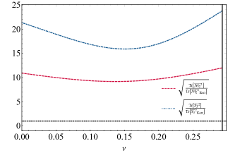
Figure 1: Ratios between the quadratic invariants for the first multipole moments of a fuzzball (solution $\bf C$) and a Kerr BH with the same angular momentum, as a function of $\nu=L/(12k^{2})$ with $k=1$. The vertical solid line corresponds to the upper bound $\nu_{\rm max}=1-1/\sqrt{2}$. The horizontal dotted black line refers to the fuzzball and Kerr moments being identical. The fuzzball moments are larger than the corresponding Kerr ones, which is a typical property companion .

Phenomenological implications. The above examples are representatives of some general features of this large family of solutions. In particular, the $\ell\geq 2$ multipole moments of fuzzball geometries are not necessarily spin induced as in the Kerr case, they can break axial and equatorial symmetries, and are larger than in the Kerr case. The peculiar multipolar structure and the striking deviation from the Kerr multipoles provides a portal to constrain fuzzball models with current and future observations, with both electromagnetic and GW probes Cardoso:2019rvt .

By analyzing the accretion flow near the supermassive BH in M87, the Event Horizon Telescope placed a mild bound on its dimensionless (axisymmetric) quadrupole moment, $|\overline{\cal M}_{2}-\overline{\cal M}_{2}^{\rm BH}|\lesssim 4$ Akiyama:2019cqa . Furthermore, in a coalescence the quadrupole moment of the binary components affect the GW signal through a next-to-next to leading post-Newtonian correction Blanchet:2006zz ; Krishnendu:2017shb . Constraints on parametrized post-Newtonian deviations using the events from the first LIGO-Virgo Catalog LIGOScientific:2018mvr ; LIGOScientific:2019fpa can be mapped into a constraint $|\overline{\cal M}_{2}-\overline{\cal M}_{2}^{\rm BH}|\lesssim 1$, in particular using the events GW151226 and GW170608 DiPasquaInPrep . Comparing with deviations found in the microstate solutions, current bounds are not particularly stringent.

While current GW constraints will become slightly more stringent in the next years as the sensitivity of the ground-based detectors improve Krishnendu:2018nqa , much tighter bounds will come from extreme mass-ratio inspirals (EMRIs), one of the main targets of the future space mission LISA Audley:2017drz . Although EMRI data analysis is challenging Babak:2017tow ; Chua:2018yng ; Chua:2019wgs ; LISADataChallenge the potential reward is unique: a detection of these systems can be used to measure the ($m=0$, mass) quadrupole moment $\overline{{\cal M}}_{2}$ of the central supermassive object with an accuracy of one part in $10^{4}$ Barack:2006pq ; Babak:2017tow , offering unprecedented tests of exotic compact objects Glampedakis:2005cf ; Raposo:2018xkf ; Destounis:2020kss .

While our results suggest that very strong constraints on fuzzball geometries can be set with EMRIs, a precise analysis requires a class of neutral, nonextremal solutions, which would further imply the absence of extra emission channels (e.g. dipolar radiation). For astrophysically viable objects, we expect that the multipolar structure is the only discriminant with respect to the Kerr BH case, which can be explored with the methods presented here.

In addition to having a different quadrupole moment, microstate geometries are much less symmetric than the Kerr metric, which implies the existence of multipole moments that are identically zero in the Kerr case (see also Refs. Ryan:1995wh ; Raposo:2018xkf ). Investigating how multipole moments that break equatorial symmetry or axisymmetry (e.g., ${\cal S}_{2m}$ and ${\cal M}_{2m}$ with $m\neq 0$) affect the GW waveform and their phenomenological consequences is an important topic that is left for a follow-up work.

Finally, a broad statistical analysis shows that certain invariant combinations of the $\ell\geq 2$ multipole moments of three-center microstate geometries are larger than those of the corresponding Kerr BH in a wide region of the four-dimensional parameter space, and are always larger than their corresponding value in the $L\to 0$ limit companion . If confirmed, this result would imply that any future measurement of the invariant combinations of the multipole moments smaller than the BH ones can potentially rule out this family of solutions to be typical microstates of the corresponding BH, with important consequences for the fuzzball scenario.

Note added. While this work was in preparation, a related work by Iosif Bena and Daniel R. Mayerson appeared Bena:2020see (see also the more recent companion Bena:2020uup ). The idea and aims of that paper are similar to ours. Ref. Bena:2020see focuses on axisymmetric geometries in the BH limit, whereas our results are valid beyond axial symmetry in regions where the microstate geometries can significantly deviate from the BH metric.

Acknowledgments. D.C. was supported by FWF Austrian Science Fund via the SAP P30531-N27. P.P. acknowledges financial support provided under the European Union’s H2020 ERC, Starting Grant agreement no. DarkGRA–757480, and under the MIUR PRIN and FARE programmes (GW-NEXT, CUP: B84I20000100001), and support from the Amaldi Research Center funded by the MIUR program “Dipartimento di Eccellenza” (CUP: B81I18001170001).

References

- (1) B. Carter, “Axisymmetric black hole has only two degrees of freedom,” Phys. Rev. Lett. 26 (Feb, 1971) 331–333. http://link.aps.org/doi/10.1103/PhysRevLett.26.331.
- (2) S. Hawking and G. Ellis, The Large Scale Structure of Space-Time. Cambridge Monographs on Mathematical Physics. Cambridge University Press, 2, 2011.
- (3) M. Heusler, “Stationary black holes: Uniqueness and beyond,” Living Rev. Relativity 1 no. 6, (1998) . http://www.livingreviews.org/lrr-1998-6.
- (4) P. T. Chrusciel, J. L. Costa, and M. Heusler, “Stationary Black Holes: Uniqueness and Beyond,” Living Rev.Rel. 15 (2012) 7, arXiv:1205.6112 [gr-qc].
- (5) D. Robinson, Four decades of black holes uniqueness theorems. Cambridge University Press, 2009.
- (6) R. Hansen, “Multipole moments of stationary space-times,” J.Math.Phys. 15 (1974) 46–52.
- (7) R. P. Geroch, “Multipole moments. II. Curved space,” J.Math.Phys. 11 (1970) 2580–2588.
- (8) P. Pani, “I-Love-Q relations for gravastars and the approach to the black-hole limit,” Phys. Rev. D 92 no. 12, (2015) 124030, arXiv:1506.06050 [gr-qc]. [Erratum: Phys.Rev.D 95, 049902 (2017)].
- (9) G. Raposo, P. Pani, and R. Emparan, “Exotic compact objects with soft hair,” Phys. Rev. D 99 no. 10, (2019) 104050, arXiv:1812.07615 [gr-qc].
- (10) D. Psaltis, “Probes and Tests of Strong-Field Gravity with Observations in the Electromagnetic Spectrum,” arXiv:0806.1531 [astro-ph].
- (11) J. R. Gair, M. Vallisneri, S. L. Larson, and J. G. Baker, “Testing General Relativity with Low-Frequency, Space-Based Gravitational-Wave Detectors,” Living Rev.Rel. 16 (2013) 7, arXiv:1212.5575 [gr-qc].
- (12) N. Yunes and X. Siemens, “Gravitational-Wave Tests of General Relativity with Ground-Based Detectors and Pulsar Timing-Arrays,” Living Rev.Rel. 16 (2013) 9, arXiv:1304.3473 [gr-qc].
- (13) E. Berti et al., “Testing General Relativity with Present and Future Astrophysical Observations,” Class. Quant. Grav. 32 (2015) 243001, arXiv:1501.07274 [gr-qc].
- (14) V. Cardoso and L. Gualtieri, “Testing the black hole no-hair hypothesis,” Class. Quant. Grav. 33 no. 17, (2016) 174001, arXiv:1607.03133 [gr-qc].
- (15) L. Barack et al., “Black holes, gravitational waves and fundamental physics: a roadmap,” Class. Quant. Grav. 36 no. 14, (2019) 143001, arXiv:1806.05195 [gr-qc].
- (16) V. Cardoso and P. Pani, “Testing the nature of dark compact objects: a status report,” Living Rev. Rel. 22 no. 1, (2019) 4, arXiv:1904.05363 [gr-qc].
- (17) T. Hertog and J. Hartle, “Observational Implications of Fuzzball Formation,” Gen. Rel. Grav. 52 no. 7, (2020) 67, arXiv:1704.02123 [hep-th].
- (18) B. Guo, S. Hampton, and S. D. Mathur, “Can we observe fuzzballs or firewalls?,” JHEP 07 (2018) 162, arXiv:1711.01617 [hep-th].
- (19) LIGO Scientific, Virgo Collaboration, R. Abbott et al., “GW190814: Gravitational Waves from the Coalescence of a 23 Solar Mass Black Hole with a 2.6 Solar Mass Compact Object,” Astrophys. J. 896 no. 2, (2020) L44, arXiv:2006.12611 [astro-ph.HE].
- (20) LIGO Scientific, Virgo Collaboration, R. Abbott et al., “GW190521: A Binary Black Hole Merger with a Total Mass of ,” Phys. Rev. Lett. 125 (2020) 101102, arXiv:2009.01075 [gr-qc].
- (21) LIGO Scientific, Virgo Collaboration, R. Abbott et al., “Properties and astrophysical implications of the 150 Msun binary black hole merger GW190521,” Astrophys. J. Lett. 900 (2020) L13, arXiv:2009.01190 [astro-ph.HE].
- (22) R. Penrose, “Gravitational collapse: The role of general relativity,” Riv. Nuovo Cim. 1 (1969) 252–276. [Gen. Rel. Grav.34,1141(2002)].
- (23) R. M. Wald, “Gravitational collapse and cosmic censorship,” in Black Holes, Gravitational Radiation and the Universe: Essays in Honor of C.V. Vishveshwara, pp. 69–85. 1997. arXiv:gr-qc/9710068 [gr-qc].
- (24) R. Penrose, “Singularities of Spacetime (in Theoretical Principles in Astrophysics and Relativity),” in Chicago University Press, Chicago, 1978 217 P. 1978.
- (25) J. D. Bekenstein, “Black holes and entropy,” Physical Review D 7 no. 8, (1973) 2333.
- (26) S. W. Hawking, “Black Holes and Thermodynamics,” Phys. Rev. D13 (1976) 191–197.
- (27) S. Hawking, “Particle Creation by Black Holes,” Commun. Math. Phys. 43 (1975) 199–220. [Erratum: Commun.Math.Phys. 46, 206 (1976)].
- (28) S. D. Mathur, “The Information paradox: A Pedagogical introduction,” Class. Quant. Grav. 26 (2009) 224001, arXiv:0909.1038 [hep-th].
- (29) A. Strominger and C. Vafa, “Microscopic origin of the Bekenstein-Hawking entropy,” Phys. Lett. B 379 (1996) 99–104, arXiv:hep-th/9601029.
- (30) G. T. Horowitz, J. M. Maldacena, and A. Strominger, “Nonextremal black hole microstates and U duality,” Phys. Lett. B 383 (1996) 151–159, arXiv:hep-th/9603109.
- (31) J. M. Maldacena, A. Strominger, and E. Witten, “Black hole entropy in M theory,” JHEP 12 (1997) 002, arXiv:hep-th/9711053.
- (32) O. Lunin and S. D. Mathur, “AdS / CFT duality and the black hole information paradox,” Nucl. Phys. B 623 (2002) 342–394, arXiv:hep-th/0109154.
- (33) O. Lunin and S. D. Mathur, “Statistical interpretation of Bekenstein entropy for systems with a stretched horizon,” Phys. Rev. Lett. 88 (2002) 211303, arXiv:hep-th/0202072.
- (34) S. D. Mathur, “The Fuzzball proposal for black holes: An Elementary review,” Fortsch. Phys. 53 (2005) 793–827, arXiv:hep-th/0502050.
- (35) S. D. Mathur, “Fuzzballs and the information paradox: A Summary and conjectures,” arXiv:0810.4525 [hep-th].
- (36) M. Bianchi, D. Consoli, and J. Morales, “Probing Fuzzballs with Particles, Waves and Strings,” JHEP 06 (2018) 157, arXiv:1711.10287 [hep-th].
- (37) M. Bianchi, D. Consoli, A. Grillo, and J. F. Morales, “The dark side of fuzzball geometries,” JHEP 05 (2019) 126, arXiv:1811.02397 [hep-th].
- (38) I. Bena, E. J. Martinec, R. Walker, and N. P. Warner, “Early Scrambling and Capped BTZ Geometries,” JHEP 04 (2019) 126, arXiv:1812.05110 [hep-th].
- (39) I. Bena, P. Heidmann, R. Monten, and N. P. Warner, “Thermal Decay without Information Loss in Horizonless Microstate Geometries,” SciPost Phys. 7 no. 5, (2019) 063, arXiv:1905.05194 [hep-th].
- (40) M. Bianchi, A. Grillo, and J. F. Morales, “Chaos at the rim of black hole and fuzzball shadows,” JHEP 05 (2020) 078, arXiv:2002.05574 [hep-th].
- (41) I. Bena, S. Giusto, R. Russo, M. Shigemori, and N. P. Warner, “Habemus Superstratum! A constructive proof of the existence of superstrata,” JHEP 05 (2015) 110, arXiv:1503.01463 [hep-th].
- (42) I. Bena, E. Martinec, D. Turton, and N. P. Warner, “Momentum Fractionation on Superstrata,” JHEP 05 (2016) 064, arXiv:1601.05805 [hep-th].
- (43) I. Bena, S. Giusto, E. J. Martinec, R. Russo, M. Shigemori, D. Turton, and N. P. Warner, “Smooth horizonless geometries deep inside the black-hole regime,” Phys. Rev. Lett. 117 no. 20, (2016) 201601, arXiv:1607.03908 [hep-th].
- (44) I. Bena, S. Giusto, E. J. Martinec, R. Russo, M. Shigemori, D. Turton, and N. P. Warner, “Asymptotically-flat supergravity solutions deep inside the black-hole regime,” JHEP 02 (2018) 014, arXiv:1711.10474 [hep-th].
- (45) M. Bianchi, J. F. Morales, L. Pieri, and N. Zinnato, “More on microstate geometries of 4d black holes,” JHEP 05 (2017) 147, arXiv:1701.05520 [hep-th].
- (46) I. Bena, D. Turton, R. Walker, and N. P. Warner, “Integrability and Black-Hole Microstate Geometries,” JHEP 11 (2017) 021, arXiv:1709.01107 [hep-th].
- (47) S. Giusto, J. F. Morales, and R. Russo, “D1D5 microstate geometries from string amplitudes,” JHEP 03 (2010) 130, arXiv:0912.2270 [hep-th].
- (48) S. Giusto, R. Russo, and D. Turton, “New D1-D5-P geometries from string amplitudes,” JHEP 11 (2011) 062, arXiv:1108.6331 [hep-th].
- (49) M. Bianchi, J. F. Morales, and L. Pieri, “Stringy origin of 4d black hole microstates,” JHEP 06 (2016) 003, arXiv:1603.05169 [hep-th].
- (50) M. Bianchi, D. Consoli, A. Grillo, J. F. Morales, P. Pani, and G. Raposo, “The multipolar structure of fuzzballs,” arXiv:2008.01445 [hep-th].
- (51) K. Thorne, “Multipole Expansions of Gravitational Radiation,” Rev.Mod.Phys. 52 (1980) 299–339.
- (52) Y. Gursel, “Multipole moments for stationary systems: The equivalence of the geroch-hansen formulation and the thorne formulation,” General Relativity and Gravitation 15 no. 8, (1983) 737–754. http://dx.doi.org/10.1007/BF01031881.
- (53) I. Bena and N. P. Warner, “Black holes, black rings and their microstates,” Lect. Notes Phys. 755 (2008) 1–92, arXiv:hep-th/0701216.
- (54) G. Gibbons and N. Warner, “Global structure of five-dimensional fuzzballs,” Class. Quant. Grav. 31 (2014) 025016, arXiv:1305.0957 [hep-th].
- (55) B. Bates and F. Denef, “Exact solutions for supersymmetric stationary black hole composites,” JHEP 11 (2011) 127, arXiv:hep-th/0304094.
- (56) E. T. Newman, R. Couch, K. Chinnapared, A. Exton, A. Prakash, and R. Torrence, “Metric of a Rotating, Charged Mass,” J. Math. Phys. 6 (1965) 918–919.
- (57) T. P. Sotiriou and T. A. Apostolatos, “Corrected multipole moments of axisymmetric electrovacuum spacetimes,” Class. Quant. Grav. 21 (2004) 5727–5733, arXiv:gr-qc/0407064.
- (58) Event Horizon Telescope Collaboration, K. Akiyama et al., “First M87 Event Horizon Telescope Results. I. The Shadow of the Supermassive Black Hole,” Astrophys. J. 875 no. 1, (2019) L1.
- (59) L. Blanchet, “Gravitational radiation from post-Newtonian sources and inspiralling compact binaries,” Living Rev. Rel. 9 (2006) 4.
- (60) N. V. Krishnendu, K. G. Arun, and C. K. Mishra, “Testing the binary black hole nature of a compact binary coalescence,” Phys. Rev. Lett. 119 no. 9, (2017) 091101, arXiv:1701.06318 [gr-qc].
- (61) LIGO Scientific, Virgo Collaboration, B. Abbott et al., “GWTC-1: A Gravitational-Wave Transient Catalog of Compact Binary Mergers Observed by LIGO and Virgo during the First and Second Observing Runs,” Phys. Rev. X 9 no. 3, (2019) 031040, arXiv:1811.12907 [astro-ph.HE].
- (62) LIGO Scientific, Virgo Collaboration, B. Abbott et al., “Tests of General Relativity with the Binary Black Hole Signals from the LIGO-Virgo Catalog GWTC-1,” Phys. Rev. D 100 no. 10, (2019) 104036, arXiv:1903.04467 [gr-qc].
- (63) F. Di Pasqua, A. Maselli, and P. Pani, “Testing the Kerr hypothesis: electromagnetic versus gravitational-wave constraints of the quadrupole moment (in preparation),”.
- (64) N. V. Krishnendu, C. K. Mishra, and K. G. Arun, “Spin-induced deformations and tests of binary black hole nature using third-generation detectors,” Phys. Rev. D99 no. 6, (2019) 064008, arXiv:1811.00317 [gr-qc].
- (65) LISA Collaboration, P. Amaro-Seoane et al., “Laser Interferometer Space Antenna,” arXiv:1702.00786 [astro-ph.IM].
- (66) S. Babak, J. Gair, A. Sesana, E. Barausse, C. F. Sopuerta, C. P. L. Berry, E. Berti, P. Amaro-Seoane, A. Petiteau, and A. Klein, “Science with the space-based interferometer LISA. V: Extreme mass-ratio inspirals,” Phys. Rev. D95 no. 10, (2017) 103012, arXiv:1703.09722 [gr-qc].
- (67) A. J. Chua, S. Hee, W. J. Handley, E. Higson, C. J. Moore, J. R. Gair, M. P. Hobson, and A. N. Lasenby, “Towards a framework for testing general relativity with extreme-mass-ratio-inspiral observations,” Mon. Not. Roy. Astron. Soc. 478 no. 1, (2018) 28–40, arXiv:1803.10210 [gr-qc].
- (68) A. J. K. Chua, N. Korsakova, C. J. Moore, J. R. Gair, and S. Babak, “Gaussian processes for the interpolation and marginalization of waveform error in extreme-mass-ratio-inspiral parameter estimation,” Phys. Rev. D101 no. 4, (2020) 044027, arXiv:1912.11543 [astro-ph.IM].
- (69) LISA Data Challenge Working Group. LISA Data Challenges, 2019. https://lisa-ldc.lal.in2p3.fr.
- (70) L. Barack and C. Cutler, “Using LISA EMRI sources to test off-Kerr deviations in the geometry of massive black holes,” Phys. Rev. D75 (2007) 042003, arXiv:gr-qc/0612029 [gr-qc].
- (71) K. Glampedakis and S. Babak, “Mapping spacetimes with LISA: Inspiral of a test-body in a ‘quasi-Kerr’ field,” Class. Quant. Grav. 23 (2006) 4167–4188, arXiv:gr-qc/0510057.
- (72) K. Destounis, A. G. Suvorov, and K. D. Kokkotas, “Testing spacetime symmetry through gravitational waves from extreme-mass-ratio inspirals,” arXiv:2009.00028 [gr-qc].
- (73) F. D. Ryan, “Gravitational waves from the inspiral of a compact object into a massive, axisymmetric body with arbitrary multipole moments,” Phys. Rev. D52 (1995) 5707–5718.
- (74) I. Bena and D. R. Mayerson, “A New Window into Black Holes,” arXiv:2006.10750 [hep-th].
- (75) I. Bena and D. R. Mayerson, “Black Holes Lessons from Multipole Ratios,” arXiv:2007.09152 [hep-th].