Creation of Universes from the Third-Quantized Vacuum

Abstract

We calculate the average numbers of closed, flat, and open universes spontaneously created from nothing in third quantization. The creation of universes is exponentially suppressed for large values of the kinetic energy of the inflaton, while for small kinetic energies it is exponentially favoured for closed universes over flat and open ones: For a scale of inflation less than about $2\times 10^{16}$GeV, the ratio of the number of closed universes to either the number of flat or open universes is

$$\frac{n_{closed}}{n_{flat,open}}\gtrsim 10^{10^{10}}.$$

I I. Introduction

In their seminal paper Hosoya-Morikawa , Hosoya and Morikawa explored the consequences of the quantization of the wave function of the Universe, now known as third quantization. The main motivation was to overcome the problem of the probabilistic interpretation of the wave function of the Universe, solution of the Wheeler-DeWitt equation: since the latter is a hyperbolic second-order differential equation, it does not admit conserved quantities that are positive definite. Their proposal of a quantum field theory of the Universe resembles to the one that successfully solved the problem of negative probability in the case of the Klein-Gordon equation.

As a consequence of their investigation, Hosoya and Morikawa discovered that universes are spontaneously created from “nothing” (the third-quantized vacuum), in the same way particles can be created from vacuum if the external potential is time dependent. In third-quantization, the time-dependent potential (the Wheeler-DeWitt potential) naturally arises from Einstein gravity, and the time variable is played by the (logarithm) of the expansion parameter.

In their paper, Hosoya and Morikawa calculated the average number of flat universes created from nothing in the presence of an homogeneous scalar field (the inflaton). Recently enough, Kim Kim calculated the number of closed and open universes in the case of vanishing potential of the scalar field. The aim of this paper is to evaluate this number in the general case of nonvanishing scalar potential.

The plan of the paper is as follows. In Sec. II, we briefly review third quantization in minisuperspace and in particular the mechanism of creation of universes from nothing. In Sec. III, an analogy between universe creation and quantum potential scattering is analyzed. This analogy will allow us to use standard WKB methods used in quantum mechanics for the calculation of the number of cerated universes. In Sections IV, V, and VI, we calculate the average numbers of flat, closed, and open universes created out of nothing in the particular case of constant scalar potential, both using WKB approximation and an approximate form of the Wheeler-DeWitt potential. In Sec. VII, we discuss our result and we draw our conclusions.

II II. Third quantization and the creation of universes from nothing

II.1 IIa. Nothingness and multiverse

The Wheeler-DeWitt equation in homogeneous and isotropic minisuperspace is (using the units $\hbar=c=4\pi G/3=1$)

$$\left[\frac{\partial^{2}}{\partial\alpha^{2}}-\frac{\partial^{2}}{\partial\phi^{2}}+U(\alpha,\phi)\right]\!\Psi(\alpha,\phi)=0,$$ (1)

where $\alpha=\ln a$, with $a$ being the expansion parameter, $\phi$ is a real scalar field (which we identify as the inflaton), $k$ is the signature of the spatial curvature, and

$$U(\alpha,\phi)=V^{2}e^{4\alpha}\left[2V(\phi)e^{2\alpha}-k\right]$$ (2)

is the Wheeler-DeWitt potential. The spatial volume $V$ is equal to $2\pi^{2}$ for closed universes ($k=1$). For flat ($k=0$) and open ($k=-1$) universes, $V$ is a normalization volume that can be taken as the (finite) volume of the region under consideration.

In third quantization, the “Universe field” $\Psi(\alpha,\phi)$ is expanded in normal modes with the coefficients of expansions being the annihilation and creation operators. A Fock space can be constructed starting from a vacuum state which represents a state of nothing, a state in which even space-time does not exist.

Following Hosoya-Morikawa , we assume that the Universe is a neutral scalar. In this case, we can write the Universe wave function in the in-Fock space as

$$\Psi(\alpha,\phi)=\int\!\!\frac{dp}{2\pi}\!\left(c_{p}\,\psi_{p}(\alpha)\,e^{ip\phi}+c_{p}^{{\dagger}}\,\psi_{p}^{*}(\alpha)\,e^{-ip\phi}\right)\!,$$ (3)

where the subscript $p$ labels the mode function and its physical meaning will be discussed later. Here, the annihilation and creation operators $c_{p}$ and $c_{p}^{{\dagger}}$ satisfy the usual commutation relations, $[c_{p},c_{p^{\prime}}^{{\dagger}}]=2\pi\delta_{pp^{\prime}}$ and $[c_{p},c_{p^{\prime}}]=[c_{p}^{{\dagger}},c_{p^{\prime}}^{{\dagger}}]=0$. The functions $\psi_{p}(\alpha)$ are positive frequency solutions (with respect to $\alpha$) of the Schrodinger-like equation

$$\ddot{\psi}_{p}=U_{p}\psi_{p},$$ (4)

where a dot indicates a derivative with respect to $\alpha$, and

$$U_{p}(\alpha)=-p^{2}-V^{2}e^{4\alpha}\left(2V_{0}e^{2\alpha}-k\right)\!.$$ (5)

Hereafter, we consider only the case of a constant scalar potential $V(\phi)=V_{0}$. Also, we assume $V_{0}\neq 0$ throughout the paper, with the expection of Section VIa, where we discuss the case of open universes with vanishing scalar potential.

In order to have a self-consistent quantization, the mode $\psi_{p}(\alpha)$ must satisfy the Wronskian condition $\psi_{p}\dot{\psi}_{p}^{*}-\dot{\psi}_{p}\psi_{p}^{*}=i$.

The vacuum state $|0\rangle$ is defined by

$$\forall p\in\mathbb{R}\!:~{}c_{p}|0\rangle=0~{}~{}\mbox{(nothinghness)}$$ (6)

and is normalized as $\langle 0|0\rangle=1$. The state $c_{p}^{{\dagger}}|0\rangle$ represents the single universe, the state $c_{p}^{{\dagger}}c_{p^{\prime}}^{{\dagger}}|0\rangle$ represents a double universe and, in general, the state

$$\prod_{i=1}^{N}c_{p_{i}}^{{\dagger}}|0\rangle~{}~{}\mbox{(multiverse)}$$ (7)

represents the multiverse, namely a state with $N$ universes each of them labeled by $p_{i}$.

II.2 IIb. Universes from nothing

As in the case of quantum field theory in curved spacetime, the vacuum state is not unique. Different inequivalent physical vacua can be introduced in different region in minisuperspace. In particular, we can define in- and out-regions for $\alpha\rightarrow-\infty$ and $\alpha\rightarrow+\infty$, respectively, to which there corresponds in- and out-vacuum states.

The in-vacuum state contains no in-universes in the in-region. Such a “Bunch-Davies vacuum” can be constructed by solving the Wheeler-DeWitt equation for the Universe states and then by fixing the constants of integrations appearing in the general solution by matching the latter with the corresponding adiabatic solution for $\alpha\rightarrow-\infty$. Accordingly, we can construct the in-Fock space based on the in-vacuum by repeatedly applying the in-creation operator on the in-vacuum state. Another Fock state can be constructed in this way, but this time starting from a out-region $\alpha\rightarrow+\infty$.

It is clear from the above discussion that the two Fock spaces based on the two different choices of the (Bunch-Davies) vacuum state are both physically acceptable and must be then related. In particular, there will be a relation between the in- and out-modes $\psi_{p}^{({\rm in})}$ and $\psi_{p}^{({\rm out})}$, as well as a relation between the in- and out-creation and annihilation operators. In order to find these relations, let us observe that if $\psi_{p}^{(1)}$ and $\psi_{p}^{(2)}$ are two solutions of Eq. (4), the following inner product is conserved,

$$\langle\psi_{p}^{(1)}|\psi_{p}^{(2)}\rangle=-i(\psi_{p}^{(1)}\dot{\psi}_{p}^{(2)}-\dot{\psi}_{p}^{(1)}\psi_{p}^{(2)}).$$ (8)

We can then introduce the time-independent quantities

$$\alpha_{p}=\langle\psi_{p}^{({\rm in})}|\psi_{p}^{({\rm out})*}\rangle,$$ (9)

$$\beta_{p}=-\langle\psi_{p}^{({\rm in})}|\psi_{p}^{({\rm out})}\rangle,$$ (10)

and expand the in-$\psi$ mode in terms of the out-$\psi$ mode as

$$\psi_{p}^{({\rm in})}=\alpha_{p}\psi_{p}^{({\rm out})}+\beta_{p}\psi_{p}^{({\rm out})*},$$ (11)

where we used the fact that

$$\langle\psi_{p}^{({\rm in})}|\psi_{p}^{({\rm in})*}\rangle=\langle\psi_{p}^{({\rm out})}|\psi_{p}^{({\rm out})*}\rangle=1.$$ (12)

Equation (11) is the wanted relation between the $\psi$ in- and out- modes. A relation of this type is know as Bogolubov transformation and the quantities $\alpha_{p}$ and $\beta_{p}$ are called Bogolubov coefficients. They satisfy the relation

$$|\alpha_{p}|^{2}-|\beta_{p}|^{2}=1,$$ (13)

which can be easily derived from their defining equations. To find the relation between the in- and out-creation and annihilation operators, we insert the Bogolubov transformation in Eq. (3) and compare the result with the the expression of $\Psi$ defined in the out-Fock space. We find $c_{p}^{({\rm out})}=\alpha_{p}\,c_{p}^{({\rm in})}-\beta_{p}^{*}\,c_{-p}^{({\rm in}){\dagger}}$. From the above equation, it follows immediately that the two Fock spaces based on the two choices $|0,{\rm in}\rangle$ and $|0,{\rm out}\rangle$ of the vacuum are generally different. In particular, the in-vacuum state will contain out-universes as long as $\beta_{p}\neq 0$,

$$n_{p}=\langle 0,{\rm in}|N^{({\rm out})}_{p}|0,{\rm in}\rangle=|\beta_{p}|^{2},$$ (14)

where $N^{({\rm out})}_{p}=c_{p}^{({\rm out}){\dagger}}c_{p}^{({\rm out})}$ is the number operator in the out-Fock space. Note that universes are created in pairs with opposite $p$.

II.3 IIc. Labeling universes

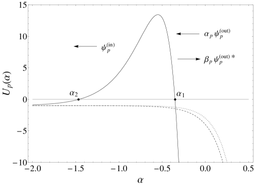
Figure 1: The Wheeler-DeWitt potential $U_{p}(\alpha)$ in Eq. (5) for $p=V_{0}=1$ and $k=1$ (continuous line), $k=-1$ (dashed line), and $k=0$ (dotted line). For open and flat universes, the volume $V$ has been taken equal to unity. The points $\alpha_{1}$ and $\alpha_{2}$ are the classical turning points in the WKB picture discussed in Section III.

Classically, the canonical momentum conjugate to $\phi$ is given by $p_{\phi}^{({\rm cl})}=Va^{3}d\phi/dt$ Hosoya-Morikawa . Accordingly, $p$ is related to the kinetic energy (density) of the scalar field, $K_{\phi}$, through

$$K_{\phi}=\frac{1}{2}\!\left(\!\frac{d\phi}{dt}\right)^{\!2}=\frac{p^{2}}{2Va^{3}}\,.$$ (15)

Thus, $p$ essentially labels universes with different amounts of kinetic energy of the inflaton. In the out-region, where the created universes behave classically, the expansion is governed by the usual Friedmann equation

$$H^{2}=\left(\!\frac{d\phi}{dt}\right)^{\!2}+2V(\phi)-\frac{k}{a^{2}}\,,$$ (16)

where $H=(da/dt)/a$ is the Hubble parameter. Taking into account Eq. (15), the Friedmann equation takes the form

$$H^{2}=\frac{p^{2}}{V^{2}a^{6}}+2V_{0}-\frac{k}{a^{2}}=-\frac{U_{p}(\alpha)}{V^{2}e^{6\alpha}}\,,$$ (17)

where $U_{p}(\alpha)$ is given by Eq. (5) for the case of constant scalar potential (see Fig. 1).

Flat universes. – For flat universes, the solution of Eq. (17) with $a(0)=0$ is easily found,

$$a(t)=\left(\frac{|p|t}{V}\right)^{\!1/3}\!\sinh(3t/a_{\rm cr}),$$ (18)

where we have defined

$$a_{\rm cr}=1/\sqrt{2V_{0}}.$$ (19)

The above expression for the expansion parameter is well approximated by

$$a(t)\!\! \simeq \!\!\left\{\begin{array}[]{lll}\!\!\left(\frac{|p|t}{V}\right)^{\!1/3}\!,&~{}a\lesssim a_{\rm cr}r^{1/6},\\ \\ \!\!\left(\frac{|p|a_{\rm cr}}{V}\right)^{\!1/3}e^{t/a_{\rm cr}-1},&~{}a\gtrsim a_{\rm cr}r^{1/6},\end{array}\right.$$ (23)

where

$$r=\left(\!\frac{p}{Va_{\rm cr}^{2}}\!\right)^{\!2}\!.$$ (24)

Thus, flat universes created in the out region with sufficiently large expansion parameter, $a\gtrsim a_{\rm cr}r^{1/6}$, undergo inflation, $a(t)\propto e^{\sqrt{2V_{0}}t}$, while those created with small expansion parameter, $a\lesssim a_{\rm cr}r^{1/6}$, are dominated by the kinetic energy of the scalar field, $a(t)\propto t^{1/3}$, and do not inflate (see the upper panel of Fig. 2).

Closed universes. – Closed universes are created in the out region only if $\alpha>\alpha_{1}$ (corresponding to $H^{2}>0$), where $\alpha_{1}$ is the largest zero of the potential $U_{p}(\alpha)$ (see Fig. 1). This corresponds to expansion parameters $a>\sqrt{x_{1}}a_{\rm cr}$, where $x_{1}$ is defined in Eq. (60). If $a<\sqrt{x_{1}}a_{\rm cr}$, the square of the Hubble parameter is negative, which indicates a recollapsing universe. This analysis is true when $r<4/27$ (see discussion in Section V), while for $r>4/27$ universes with any value of $a$ can be created. Using the results of Section V (see in particular Fig. 3), the root $x_{1}(r)$ is in the interval $2/3<x_{1}(r)<1$ for $0<r<4/27$. For the sake of simplicity and convenience, let us assume that created universes recollapse when $a\lesssim a_{\rm cr}$ for $r\lesssim 1$. Assuming that either $a\gtrsim a_{\rm cr}$ or $r\gtrsim 1$, the expression for the expansion parameter can be approximated as

$$a(t)\!\! \simeq \!\!\left\{\begin{array}[]{lll}\!\!\left(\frac{|p|t}{V}\right)^{\!1/3}\!,&~{}a\lesssim a_{\rm cr}r^{1/6},~{}r\gtrsim 1,\\ \\ \!\!\left(\frac{|p|a_{\rm cr}}{V}\right)^{\!1/3}e^{t/a_{\rm cr}-1},&~{}a\gtrsim a_{\rm cr}\max[1,r^{1/6}].\end{array}\right.$$ (28)

The upper branch of $a(t)$ in the above equation corresponds to the case of a dominant kinetic term in the Hubble parameter, while the lower branch to the case of a dominant potential term. In the former case, universes inflate, in the latter they do not (see the middle panel of Fig. 2).

Open universes. – For open universes, the approximated solution of Eq. (17) reads

$$a(t)\!\! \simeq \!\!\left\{\begin{array}[]{lll}\!\!\left(\frac{|p|t}{V}\right)^{\!1/3}\!,&~{}a\lesssim a_{\rm cr}r^{1/4},~{}r\lesssim 1,~{}\mbox{or}\\ &~{}a\lesssim a_{\rm cr}r^{1/6},~{}r\gtrsim 1,\\ \\ \!\!\left(\frac{|p|a_{\rm cr}}{V}\right)^{\!1/3}e^{t/a_{\rm cr}-1},&~{}a\gtrsim a_{\rm cr},~{}r\lesssim 1,~{}\mbox{or}\\ &~{}a\gtrsim a_{\rm cr}r^{1/6},~{}r\gtrsim 1,\\ \\ \!\!t,&~{}a_{\rm cr}r^{1/4}\lesssim a\lesssim a_{\rm cr},~{}r\lesssim 1.\end{array}\right.$$ (36)

The three branches correspond to a dominant kinetic, potential, and curvature term in the Hubble parameter. The lower panel of Fig. 2 graphically shows the case of open universes.

Figure 2: The expansion parameter of flat (upper panel), closed (middle panel), and open (middle panel) universes created in the out region as a function of the parameter $r$ defined by Eq. (24).

III III. Universe creation analogy with quantum potential scattering

III.1 IIIa. General considerations

The Wheeler-DeWitt equation (4) for the $\psi$ modes is formally equal to the one-dimensional Schrodinger equation with zero energy, mass equal to $1/2$, and potential energy $U_{p}(\alpha)$, with $\alpha$ taking the place of the spatial coordinate and $p$ being an external parameter. Continuing the analogy, Eq. (11) connecting the $\psi_{p}^{(\rm in)}$ and $\psi_{p}^{(\rm out)}$ modes describes the scattering of $\psi$-waves off the potential $U_{p}$, the incident, reflected, and transmitted waves being

$$\psi_{p}^{({\rm inc})}=\alpha_{p}\psi_{p}^{(\rm out)},$$ (37)

$$\psi_{p}^{({\rm ref})}=\beta_{p}\psi_{p}^{(\rm out)*},$$ (38)

$$\psi_{p}^{({\rm tr})}=\alpha_{p}\psi_{p}^{(\rm in)},$$ (39)

respectively, as illustrated in Fig. 1. Moreover, one can define a density current associated to any $\psi$-mode as

$$j_{p}=\langle\psi_{p}|\psi_{p}^{*}\rangle.$$ (40)

The conservation of the current (40), $\dot{j}_{p}=0$, follows directly from the conservation of the inner product. The incident, reflected, and transmitted currents are then

$$j_{p}^{({\rm inc})}=\langle\alpha_{p}\psi_{p}^{({\rm out})}|\alpha_{p}^{*}\psi_{p}^{({\rm out})*}\rangle=|\alpha_{p}|^{2},$$ (41)

$$j_{p}^{({\rm ref})}=\langle\beta_{p}\psi_{p}^{({\rm out})*}|\beta_{p}^{*}\psi_{p}^{({\rm out})}\rangle=-|\beta_{p}|^{2},$$ (42)

$$j_{p}^{({\rm tr})}=\langle\psi_{p}^{({\rm in})}|\psi_{p}^{({\rm in})*}\rangle=1,$$ (43)

where we used Eqs. (12).

Taking into account Eq. (14) and the Bogoliubov condition (13), we find the reflection and transmission coefficients

$$R_{p}=-\frac{j_{p}^{({\rm ref})}}{j_{p}^{({\rm inc})}}=\frac{n_{p}}{1+n_{p}}\,,$$ (45)

$$T_{p}=\frac{j_{p}^{({\rm tr})}}{j_{p}^{({\rm inc})}}=\frac{1}{1+n_{p}}\,,$$

from which the unitarity condition $R_{p}+T_{p}=1$ directly follows.

It is clear that if $p^{2}<\max U_{0}(\alpha)$, then the “particle” described by the wave function $\alpha_{p}\psi_{p}^{(\rm out)}$ will penetrate through the potential barrier $U_{p}(\alpha)$. To “particles” which deeply penetrate into the barrier, $p^{2}\ll\max U_{0}(\alpha)$, there will correspond a large reflection coefficient and, in turn, by Eq. (45), a large “particle” number $n_{p}$. On the other hand, if $p^{2}>\max U_{0}(\alpha)$, the “particle” is reflected above the barrier. For $p^{2}\gg\max U_{0}(\alpha)$, the reflection coefficient for scattering above the barrier will be small. To this case, there will correspond a small production of “particles”, $n_{p}\ll 1$.

III.2 IIIb. WKB approximation

The usefulness of Eqs. (45) and (45) resides in the fact that if the potential $U_{p}$ is slowly varying, in the sense specified below, one can apply the standard semiclassical (WKB) results for the reflection and transmission coefficients. Using the formal equivalence of the two problems of potential scattering in quantum mechanics and the creation of universes out from the vacuum in third quantization, one can then find the expression for the universe number $n_{p}$. The WKB approximation is valid whenever the potential $U_{p}$ satisfies the semiclassical condition Landau

$$\left|\frac{\dot{U}_{p}}{2U_{p}^{3/2}}\right|\ll 1.$$ (46)

It can be verified that the above condition is satisfied for the Wheeler-DeWitt potential (2) for values of $\alpha$ far from the turning points, where the WKB approximation is in general not valid.

Large universe number. – Let us consider the case of closed universes, $k>1$ (see Fig. 1). Accordingly, there will be two classical turning points, $\alpha_{2}(p)<\alpha_{1}(p)$, for a deep penetration through the potential barrier. Since in this case $R_{p}\simeq 1$, and then $T_{p}\ll 1$, we have from Eq. (45), $n_{p}\simeq T_{p}^{-1}\gg 1$. Using the standard result for the expression of the transmission coefficient in WKB approximation Landau , we find

$$n_{p}=e^{2S_{p}},$$ (47)

where

$$S_{p}=\int_{\alpha_{2}(p)}^{\alpha_{1}(p)}\!d\alpha\sqrt{U_{p}(\alpha)}\,.$$ (48)

Small universe number. – The probability that a “particle” is scattered above the potential barrier is small for large values of $p^{2}$ compared to the height of the Wheeler-DeWitt barrier $U_{0}(\alpha)$. This is true for closed, flat, and open universes. Using Eq. (45), we then have $n_{p}\simeq R_{p}\ll 1$. Using the standard result for the expression of the reflection coefficient in WKB approximation Landau , we find

$$n_{p}=e^{-4\mathrm{Im}\sigma_{p}},$$ (49)

where

$$\sigma_{p}=\int_{\alpha_{R}}^{\alpha_{I}(p)}\!d\alpha\sqrt{-U_{p}(\alpha)}\,.$$ (50)

Here, $\alpha_{I}(p)$ is the so-called imaginary turning point, the complex solution of the equation $U_{p}(\alpha)=0$ for $p^{2}>\max U_{0}(\alpha)$, and $\alpha_{R}$ is an arbitrary and inessential real parameter. The integration in Eq. (50) has to be performed in the complex upper half-plane, $\mbox{Im}[\alpha_{I}(p)]>0$. If the equation for the imaginary turning point admits more than one solution, one must select the one for which $\sigma_{p}$ is smallest Landau .

IV IV. Creation of flat inflationary universes

Exact solution. – The case $k=0$ was analyzed by Hosoya and Morikawa Hosoya-Morikawa . An exact solution for the number of created universes is given by

$$n_{p}=\frac{1}{e^{2\pi|p|/3}-1}$$ (51)

and is, interestingly enough, independent on $V_{0}$. For large $|p|$, $n_{p}$ is exponentially suppressed, while for small $|p|$, $n_{p}$ is inversely proportional to $|p|$. Equation (51) is easily found by inserting the Bunch-Davies, in- and out-solutions of Eq. (4) (with $k=0$),

$$\!\!\!\!\!\!\!\!\!\!\!\!\!\!\!\!\!\!\psi_{p}^{(\rm in)}=\sqrt{\frac{\pi}{6}}\,\sinh^{-1/2}(p\pi/3)J_{-ip/3}(V\sqrt{2V_{0}}e^{3\alpha}/3),$$ (52)

$$\!\!\!\!\!\!\!\!\!\!\!\!\!\!\!\!\!\!\psi_{p}^{(\rm out)}=\sqrt{\frac{\pi}{12}}\,e^{-p\pi/6}H_{-ip/3}^{(2)}(V\sqrt{2V_{0}}e^{3\alpha}/3),$$ (53)

into Eq. (10) and then using Eq. (14). Here, $J_{\nu}(x)$ is the Bessel function of first kind and $H_{\nu}^{(2)}(x)$ is the Hankel function of second kind Abramowitz .

Figure 3: Left panel. The functions $x_{1}(r)$, $x_{2}(r)$, and $x_{3}(r)$ in Eqs. (60)-(61) for $0\leq r\leq 4/27$. Observe that $x_{1}(4/27)=x_{2}(4/27)=2/3$ and $x_{3}(4/27)=-1/3$. Right panel. The function $f(r)$ in Eq. (64) for $0\leq r\leq 4/27$.

WKB approximation. – In this case, the WKB approximation is valid for large values of $|p|$. The imaginary turning points are

$$\alpha_{I}(p)=\frac{1}{6}\!\left[\ln(p^{2}/2V^{2}V_{0})+i\pi(2n+1)\right]\!,~{}~{}n\in\mathbb{N}.$$ (54)

Accordingly,

$$\sigma_{p}=-\frac{q}{3}+\frac{|p|}{6}\ln\!\frac{|p|+q}{|p|-q}\,,$$ (55)

where $q=\sqrt{-U_{p}(\alpha_{R})}=\sqrt{p^{2}+2V^{2}V_{0}e^{6\alpha_{R}}}$, so that $\mbox{Im}\sigma_{p}=\pi|p|/6$. It follows that

$$n_{p}=e^{-2\pi|p|/3},$$ (56)

in agreement with Eq. (51) in the case of large $|p|$.

The case of null scalar potential. – In the case of flat universes with null scalar potential, the in and out $\psi$ modes are normalized plane waves. As in the case of conformally flat quantum theories in curved space, there is no production of “particles” out from the vacuum. The number of created universes is then exactly zero.

V V. Creation of closed inflationary universes

The problem does not admit an exact analytical solution.

V.1 Va. Large universe number: small $|p|$

WKB approximation. – Let us work in WKB approximation and consider Eqs. (47) and (48). Using the change of variable $x=2V_{0}e^{2\alpha}$, the universe number can be written as

$$n_{p}=e^{2\pi^{2}f(r)/3V_{0}},$$ (57)

where $r$ is given by Eq. (24) with $V=2\pi^{2}$, and we have introduced the function

$$f(r)=\frac{3}{2}\int_{x_{2}}^{x_{1}}\frac{dx}{x}\sqrt{-x^{3}+x^{2}-r}.$$ (58)

Here, $x_{1}\geq x_{2}\geq 0$ correspond to the classical turning points, the real and positive solutions of the equation $x^{3}-x^{2}+r=0$. The three solution of such a cubic equation can be written as

$$x_{1}(r)=\frac{1}{3}\left(\!1+2\cos\frac{\theta}{3}\right)\!,$$ (60)

$$x_{2}(r)=\frac{1}{3}\left(\!1-2\cos\frac{\theta+\pi}{3}\right)\!,$$

$$x_{3}(r)=\frac{1}{3}\left(\!1-2\cos\frac{\theta-\pi}{3}\right)\!,$$ (61)

with

$$\theta(r)=\arccos(1-27r/2).$$ (62)

As it easy to check, the above three solutions are real when

$$0\leq r\leq 4/27.$$ (63)

In this case, $x_{1}$ and $x_{2}$ are positive, with $x_{1}\geq x_{2}$, and $x_{3}$ is negative (see the left panel of Fig. 3).

The integral in Eqs. (58) can be expressed in terms of the complete elliptical integrals as

$$f(r)=c_{K}K(m)+c_{E}E(m)+c_{\Pi}\Pi(n,m),$$ (64)

where

$$c_{K}=\frac{x_{3}}{\sqrt{x_{2}-x_{3}}}\,,~{}~{}c_{E}=\frac{x_{2}-x_{3}}{\sqrt{x_{2}-x_{3}}}\,,~{}~{}c_{\Pi}=\frac{3x_{1}x_{3}}{\sqrt{x_{2}-x_{3}}}\,,$$ (65)

and

$$m=\frac{x_{2}-x_{1}}{x_{2}-x_{3}}\,,~{}~{}n=\frac{x_{2}-x_{1}}{x_{2}}\,.$$ (66)

Here, $K(m)$, $E(m)$, and $\Pi(n,m)$ are the complete elliptical integrals of first, second, and third kind, respectively Abramowitz . A plot of the function $f(r)$ is shown in the right panel of Fig. 3. Notice that

$$\lim_{r\rightarrow 0}f(r)=1,~{}~{}\lim_{r\rightarrow 4/27}f(r)=0.$$ (67)

The WKB result (57) is valid only if $n_{p}\gg 1$, namely when the exponent $2\pi^{2}f(r)/3V_{0}$ is much bigger than unity. For $r\ll 1$ (the case $r\gg 1$ will be analyzed in Section Vb), this means $V_{0}\ll 2\pi^{2}/3$. In this case, we have

$$n_{p}=e^{2\pi^{2}/3V_{0}},~{}~{}|p|\ll 1\ll 2\pi^{2}/3V_{0},$$ (68)

for the average number of created universes. The case $r\ll 1$ and $V_{0}\gg 2\pi^{2}/3$, namely $|p|\ll 2\pi^{2}/3V_{0}\ll 1$, cannot be solved in WKB approximation. We proceed as follows.

Approximate Wheeler-DeWitt potential. – Let us approximate the Wheeler-DeWitt potential as

$$U_{p}(\alpha)\!\! \simeq \!\!\left\{\begin{array}[]{lll}-p^{2}+4\pi^{4}e^{4\alpha},&~{}~{}~{}~{}\alpha\leq\alpha_{\star},\\ -p^{2}-8\pi^{4}V_{0}e^{6\alpha},&~{}~{}~{}~{}\alpha>\alpha_{\star},\end{array}\right.$$ (71)

where $e^{\alpha_{\star}}=1/\sqrt{3V_{0}}$, and $\alpha_{\star}$ is the point of maximum of the Wheeler-DeWitt potential. The approximate potential (71) is discontinuous at $\alpha=\alpha_{\star}$ with a jump discontinuity of

$$\Delta=|\!\!\lim_{\alpha\rightarrow\alpha_{\star}^{-}}\!\!U_{p}(\alpha)\,-\lim_{\alpha\rightarrow\alpha_{\star}^{+}}\!\!U_{p}(\alpha)|=\frac{5}{3}\!\left(\frac{2\pi^{2}}{3V_{0}}\right)^{\!2}.$$ (72)

In the analogue case of quantum potential scattering, the reflection and transmission coefficients obtained by approximating a smooth potential with one possessing a jump discontinuity are trustworthy only if the wavelength of the incident particle is much bigger than the square root of the jump (see, e.g. Campanelli ). In our case, such a validity condition translates into the condition

$$|p|\ll\sqrt{\Delta/2}\simeq 2\pi^{2}/3V_{0}.$$ (73)

The Bunch-Davies-normalized $\psi_{p}^{({\rm in})}$ and $\psi_{p}^{({\rm out})}$ wave functions are easily found in the case of the approximate Wheeler-DeWitt potential. They are

$$\!\!\!\!\!\!\!\!\!\!\!\psi_{p}^{({\rm in})}\!\! = \!\!\left\{\begin{array}[]{lll}u_{p},&~{}~{}~{}~{}\alpha\leq\alpha_{\star},\\ c_{1}v_{p}+c_{2}v_{p}^{*},&~{}~{}~{}~{}\alpha>\alpha_{\star},\end{array}\right.$$ (76)

and

$$\!\!\!\!\!\!\!\!\!\!\!\psi_{p}^{({\rm out})}\!\! = \!\!\left\{\begin{array}[]{lll}c_{3}u_{p}+c_{4}u_{p}^{*},&~{}\alpha\leq\alpha_{\star},\\ v_{p},&~{}\alpha>\alpha_{\star},\end{array}\right.$$ (79)

respectively. Here, $u_{p}$ is given by

$$u_{p}=\frac{\Gamma(1-ip/2)}{2^{ip/2}\sqrt{2p}}\,I_{-ip/2}(\pi^{2}e^{2\alpha}),$$ (80)

where $\Gamma(x)$ is the Gamma function and $I_{\nu}(x)$ is the modified Bessel function of first kind Abramowitz . The function $u_{p}$ represents a normalized in-mode of a closed universe with $V_{0}=0$. The function $v_{p}$, instead, is given by the right hand side of Eq. (53) and represent a normalized out-mode of a flat universe with $V_{0}\neq 0$. The constants of integrations $c_{i}$ ($i=1,2,3,4$) can be found by imposing the continuity of $\psi_{p}^{({\rm in})}$ and $\psi_{p}^{({\rm out})}$, and their first derivatives, at $\alpha=\alpha_{\star}$. We find

$$c_{1}=c_{3}^{*}=\langle\psi_{p}^{({\rm in})}|\psi_{p}^{({\rm out})*}\rangle_{|\alpha=\alpha_{\star}}=\alpha_{p},$$ (81)

$$c_{2}=-c_{4}=-\langle\psi_{p}^{({\rm in})}|\psi_{p}^{({\rm out})}\rangle_{|\alpha=\alpha_{\star}}=\beta_{p}.$$ (82)

Accordingly, the average number of universes is

$$n_{p}=|\langle u_{p}|v_{p}\rangle|^{2}_{\alpha=\alpha_{\star}}.$$ (83)

For $|p|\rightarrow 0$, or more precisely for $|p|\ll\min[1,2\pi^{2}/3V_{0}]$, we find

$$n_{p}=\frac{H(V_{0}/2\pi^{2})}{\pi|p|}$$ (84)

at the leading order, where

$$\!\!\!H(x)=\frac{\pi^{2}}{1296x^{2}}$$

$$\!\!\!\times\!\left[\sqrt{6}I_{1}\!\!\left(\frac{1}{6x}\right)\!H_{0}^{(1)}\!\!\left(\frac{\sqrt{6}}{27x}\right)+2I_{0}\!\!\left(\frac{1}{6x}\right)\!H_{1}^{(1)}\!\!\left(\frac{\sqrt{6}}{27x}\right)\right]$$

$$\!\!\!\times\!\left[\sqrt{6}I_{1}\!\!\left(\frac{1}{6x}\right)\!H_{0}^{(2)}\!\!\left(\frac{\sqrt{6}}{27x}\right)+2I_{0}\!\!\left(\frac{1}{6x}\right)\!H_{1}^{(2)}\!\!\left(\frac{\sqrt{6}}{27x}\right)\right]\!,$$

with $H_{\nu}^{(1)}(x)$ being the Hankel function of first kind Abramowitz . Figure 4 shows the function $H(x)$ together with its asymptotic expansions for small and large values of the argument,

$$H(x)\!\! = \!\!\left\{\begin{array}[]{lll}\frac{5}{4\sqrt{6}}\,e^{1/3x}\left(1+\mathcal{O}(x)\right)\!,&~{}x\rightarrow 0,\\ 3/2+\mathcal{O}(1/x^{2}),&~{}x\rightarrow\infty.\end{array}\right.$$ (88)

Accordingly, the average number of created universes for small $|p|$ is

$$n_{p}\!\! \simeq \!\!\left\{\begin{array}[]{lll}\frac{5}{4\sqrt{6}\,\pi|p|}\,e^{2\pi^{2}/3V_{0}},&~{}|p|\ll 1\ll 2\pi^{2}/3V_{0},\\ \\ \frac{3}{2\pi|p|}\,,&~{}|p|\ll 2\pi^{2}/3V_{0}\ll 1.\end{array}\right.$$ (93)

The first equation in (93) is in agreement with the result (68) obtained in WKB approximation. Notice that both equations are approximate results and that, in general, the WKB approximation cannot be used to calculate the pre-exponential factor in the transmission coefficient Landau that, in our case, corresponds to the reciprocal of the average number of created universes.

It is interesting to observe that for small $|p|$ and large values of the scalar potential, $|p|\ll 2\pi^{2}/3V_{0}\ll 1$, the number of closed universes approaches the number of flat universes [see Eq.  (51)], and that the former is exponentially amplified for small scalar potentials, $|p|\ll 1\ll 2\pi^{2}/3V_{0}$.

Figure 4: The continuous and dotted lines represent, respectively, the function $H(x)$ in Eq. (V.1) and its asymptotic expansions in Eq. (88).

V.2 Vb. Small universe number: large $|p|$

WKB approximation. – The case of large $|p|$ can be only analyzed in WKB approximation (see footnote 2). For $r>4/27$, the solutions $x_{1}(r)$ and $x_{2}(3)$ are complex (conjugate), and $x_{3}(r)$ is negative. This means that the Wheeler-DeWitt potential has no classical turning points. Using Eqs. (49) and (50), we find for the average number of created universes

$$n_{p}=e^{-2\pi^{2}g(r)/3V_{0}},$$ (94)

where

$$g(r)=3\mbox{Im}\!\left[\int_{x_{R}}^{x_{1}}\frac{dx}{x}\sqrt{x^{3}-x^{2}+r}\,\right]\!.$$ (95)

Here, $x_{R}$ is a real and positive parameter, and between $x_{1}(r)$ and $x_{2}(r)$ we selected the former as the imaginary turning point since it gives the smallest $\sigma_{p}$ (see discussion in Section IIIb). Taking $x_{R}=-x_{3}(r)$, we find

$$g(r)=-2\mbox{Re}\!\left[c_{K}F(\varphi,m)+c_{E}E(\varphi,m)+c_{\Pi}\Pi(n,\varphi,m)\right]\!,$$ (96)

where $c_{K}$, $c_{E}$, and $c_{\Pi}$ are given by Eq. (65), and

$$\varphi=\arcsin\!\sqrt{(x_{2}+x_{3})/(x_{2}-x_{1})}\,.$$ (97)

Here, $F(\varphi,m)$, $E(\varphi,m)$, and $\Pi(n,\varphi,m)$ are the incomplete elliptical integrals of first, second, and third kind, respectively Abramowitz . Notice that

$$\lim_{r\rightarrow 4/27}g(r)=0.$$ (98)

A plot of $g(r)$ and its asymptotic expansion,

$$g(r)=\pi\sqrt{r}-Cr^{1/6}+\mathcal{O}(r^{-1/6}),~{}~{}r\rightarrow+\infty,$$ (99)

is shown in Fig. 5. The constant $C$ in the above equation is defined by

$$C=\frac{3z_{1}E(z_{2})-\sqrt{3}z_{1}^{*}K(z_{2})}{\sqrt{8}}\simeq 1.12025,$$ (100)

where $z_{1}=\sqrt{3+i\sqrt{3}}$ and $z_{2}=(1+i\sqrt{3})/2$. Inserting the leading term of the asymptotic expansion (99) into Eq. (94), we find

$$n_{p}\simeq e^{-2\pi|p|/3},~{}~{}|p|\gg 1,$$ (101)

for the average number of created universes. Thus, the number of closed universes is exponentially suppressed for large $|p|$, as in the case of flat universes [see Eq. (51)].

Figure 5: The function $g(r)$ in Eq. (96) for $r\geq 4/27$ with its asymptotic expansion (99).

The case of null scalar potential. – In the case of closed universes with null scalar potential, the out $\psi$ modes are exactly zero. In this case, indeed, the Wheeler-DeWitt potential grows exponentially in the out region ($\alpha\rightarrow 0$), and represents an infinite potential barrier in the analogue case of quantum potential scattering. No “particles” are present in the our region, and the number of created universes is exactly zero.

The analogy between quantum potential scattering and the creation of universes from nothing reposes on the assumption that the in and out modes are normalized according to the Bunch-Davies “prescription”, as in the case of quantum theory in curved space. This in turns follows from the fact that the procedure of third quantization closely mimics the one adopted in second quantization.

VI VI. Creation of open inflationary universes

VI.1 VIa. The case of null scalar potential

Exact solution. – The case $k=-1$ and $V_{0}=0$ was analyzed by Kim Kim . An exact solution for the number of created universes is given by

$$n_{p}=\frac{1}{e^{\pi|p|}-1}.$$ (102)

For large $|p|$, $n_{p}$ is exponentially suppressed, while for small $|p|$, $n_{p}$ is inversely proportional to $|p|$. Equation (102) is easily found by inserting the Bunch-Davies, in- and out-solutions of Eq. (4) (with $k=-1$ and $V_{0}=0$),

$$\!\!\!\!\!\!\psi_{p}^{(\rm in)}=\sqrt{\frac{\pi}{4}}\,\sinh^{-1/2}(p\pi/2)J_{-ip/2}(Ve^{2\alpha}/2),$$ (103)

$$\!\!\!\!\!\!\psi_{p}^{(\rm out)}=\sqrt{\frac{\pi}{8}}\,e^{-p\pi/4}H_{-ip/2}^{(2)}(Ve^{2\alpha}/2),$$ (104)

into Eq. (10) and then using Eq. (14).

WKB approximation. – In this case, the WKB approximation is valid for large values of $|p|$. The imaginary turning points are

$$\alpha_{I}(p)=\frac{1}{4}\left[\ln(p^{2}/V^{2})+i\pi(2n+1)\right]\!,~{}~{}n\in\mathbb{N}.$$ (105)

Accordingly,

$$\sigma_{p}=-\frac{s}{2}+\frac{|p|}{4}\ln\!\frac{|p|+s}{|p|-s}\,,$$ (106)

where $s=\sqrt{-U_{p}(\alpha_{R})}=\sqrt{p^{2}+V^{2}e^{4\alpha_{R}}}$, so that $\mbox{Im}\sigma_{p}=\pi|p|/4$. It follows that

$$n_{p}=e^{-\pi|p|},$$ (107)

in agreement with Eq. (102) in the case of large $|p|$.

VI.2 VIb. Small universe number: large $|p|$

Figure 6: Left panel. The functions $y_{1}(r)$, $y_{2}(r)$, and $y_{3}(r)$ in Eqs. (110)-(112). Right panel. The continuous and dotted lines represent, respectively, the function $k(r)$ in Eq. (114) and its asymptotic expansions in Eq. (120).

WKB approximation. – The case $k=-1$ and $V_{0}\neq 0$ cannot be solved analytically. Working in WKB approximation, we consider Eqs. (49) and (50) since, in this case, there are not classical turning points. Using the change of variable $y=2V_{0}e^{2\alpha}$, the universe number can be written as

$$n_{p}=e^{-Vk(r)/3V_{0}},$$ (108)

where

$$k(r)=3\mbox{Im}\!\left[\int_{y_{R}}^{y_{1}}\frac{dy}{y}\sqrt{y^{3}+y^{2}+r}\,\right]\!.$$ (109)

Here, $y_{R}$ is a real and positive parameter, while $y_{1}$ corresponds to the imaginary turning point, the solution of the equation $y^{3}+y^{2}+r=0$ which gives the smallest $\sigma_{p}$ in Eq. (50). The three solution of such a cubic equation can be written as

$$y_{1}=-\frac{1}{3}\left(1-2\cos\frac{\vartheta}{3}\right)\!,$$ (110)

$$y_{2}=-\frac{1}{3}\left(1+2\cos\frac{\vartheta+\pi}{3}\right)\!,$$ (111)

$$y_{3}=-\frac{1}{3}\left(1+2\cos\frac{\vartheta-\pi}{3}\right)\!,$$ (112)

with

$$\vartheta(r)=\arccos(-1-27r/2).$$ (113)

Notice that $\vartheta(r)=\pi-\theta(-r)$, $y_{1}(r)=-x_{3}(-r)$, $y_{2}(r)=-x_{2}(-r)$, and $y_{3}(r)=-x_{1}(-r)$, where $\theta(r)$ is defined in Eq. (62), and $x_{i}(r)$ are given by Eqs. (60)-(61). As it easy to check, $y_{3}$ is real and negative, while $y_{1}$ and $y_{2}$ are complex conjugate (see the left panel of Fig. 6). Taking $y_{R}=-y_{3}(r)$, the integral in Eqs. (109) can be expressed in terms of the incomplete elliptical integrals as

$$k(r)=2\mbox{Re}\!\left[C_{K}F(\omega,\mu)+C_{E}E(\omega,\mu)-C_{\Pi}\Pi(\nu,\omega,\mu)\right]\!,$$ (114)

where

$$C_{K}=\frac{y_{3}}{\sqrt{y_{2}-y_{3}}}\,,~{}~{}C_{E}=\frac{y_{2}-y_{3}}{\sqrt{y_{2}-y_{3}}}\,,~{}~{}C_{\Pi}=\frac{3y_{1}y_{3}}{\sqrt{y_{2}-y_{3}}}\,,$$ (115)

$$\mu=\frac{y_{2}-y_{1}}{y_{2}-y_{3}}\,,~{}~{}\nu=\frac{y_{2}-y_{1}}{y_{2}}\,,$$ (116)

and

$$\omega=\arcsin\!\sqrt{(y_{2}+y_{3})/(y_{2}-y_{1})}\,.$$ (117)

We show the graph of the function $k(r)$ in the right panel of Fig. 6. Also shown are the asymptotic expansions of $k(r)$ for small and large values of the argument,

$$k(r)\!\! = \!\!\left\{\begin{array}[]{lll}\frac{3}{2}\pi\sqrt{r}-\frac{3}{8}\pi r+\mathcal{O}(r^{2}),&~{}r\rightarrow 0,\\ \pi\sqrt{r}+Cr^{1/6}+\mathcal{O}(r^{-1/6}),&~{}r\rightarrow\infty,\end{array}\right.$$ (120)

where the constant $C$ is given by Eq. (100). Inserting the leading terms of the above asymptotic expansions into Eq. (108), we find

$$n_{p}\!\! \simeq \!\!\left\{\begin{array}[]{lll}e^{-\pi|p|},&~{}1\ll|p|\ll V/2V_{0},\\ e^{-2\pi|p|/3},&~{}|p|\gg\max[1,V/2V_{0}].\end{array}\right.$$ (123)

Thus, the number of open universes is exponentially suppressed for large $|p|$. If the scalar potential is small, $V/2V_{0}\gg 1$, the suppression factor is the same as in the case of open universes with null scalar potential [see Eq. (102)], while if the scalar potential is large, $V/2V_{0}\ll 1$, the suppression is similar to that of flat universes [see Eq. (51)].

VI.3 VIc. Large universe number: small $|p|$

Approximate Wheeler-DeWitt potential. – The case of small $|p|$ cannot be solved in WKB approximation. Let us proceed as in Section Va by approximating the Wheeler-DeWitt potential as

$$U_{p}(\alpha)\!\! \simeq \!\!\left\{\begin{array}[]{lll}-p^{2}-V^{2}e^{4\alpha},&~{}~{}~{}~{}\alpha\leq\alpha_{*},\\ -p^{2}-2V^{2}V_{0}e^{6\alpha},&~{}~{}~{}~{}\alpha>\alpha_{*},\end{array}\right.$$ (126)

where $e^{\alpha_{*}}=1/\sqrt{2V_{0}}$. The approximate potential is continuous at $\alpha_{*}$, while its derivative is discontinuous with a jump discontinuity of

$$\delta=|\!\!\lim_{\alpha\rightarrow\alpha_{\star}^{-}}\!\!\dot{U}_{p}(\alpha)\,-\lim_{\alpha\rightarrow\alpha_{\star}^{+}}\!\!\dot{U}_{p}(\alpha)|=\frac{V^{2}}{2V_{0}^{2}}\,.$$ (127)

As discussed in Section Va, the above approximation is trustworthy only for values of $|p|$ small compared to the square root of the jump,

$$|p|\ll\sqrt{|\alpha_{*}|\delta/2}\sim V/2V_{0}.$$ (128)

The Bunch-Davies-normalized $\psi_{p}^{({\rm in})}$ and $\psi_{p}^{({\rm out})}$ wave functions are easily found in the case of the approximate Wheeler-DeWitt potential. They are

$$\!\!\!\!\!\!\!\!\!\!\!\psi_{p}^{({\rm in})}\!\! = \!\!\left\{\begin{array}[]{lll}w_{p},&~{}~{}~{}~{}\alpha\leq\alpha_{*},\\ c_{1}v_{p}+c_{2}v_{p}^{*},&~{}~{}~{}~{}\alpha>\alpha_{*},\end{array}\right.$$ (131)

and

$$\!\!\!\!\!\!\!\!\!\!\!\psi_{p}^{({\rm out})}\!\! = \!\!\left\{\begin{array}[]{lll}c_{3}w_{p}+c_{4}w_{p}^{*},&~{}\alpha\leq\alpha_{*},\\ v_{p},&~{}\alpha>\alpha_{*},\end{array}\right.$$ (134)

respectively. Here, $w_{p}$ is given by the right hand side of Eq. (103) and represents a normalized in-mode of a open universe with $V_{0}=0$, while $v_{p}$ is given by the right hand side of Eq. (53) and represent a normalized out-mode of a flat universe with $V_{0}\neq 0$. The constants of integrations $c_{i}$ ($i=1,2,3,4$) can be found by imposing the continuity of $\psi_{p}^{({\rm in})}$ and $\psi_{p}^{({\rm out})}$, and their first derivatives, at $\alpha_{*}$. We find

$$c_{1}=c_{3}^{*}=\langle\psi_{p}^{({\rm in})}|\psi_{p}^{({\rm out})*}\rangle_{|\alpha=\alpha_{*}}=\alpha_{p},$$ (135)

$$c_{2}=-c_{4}=-\langle\psi_{p}^{({\rm in})}|\psi_{p}^{({\rm out})}\rangle_{|\alpha=\alpha_{*}}=\beta_{p}.$$ (136)

Accordingly, the average number of universes is

$$n_{p}=|\langle w_{p}|v_{p}\rangle|^{2}_{\alpha=\alpha_{*}}.$$ (137)

For $|p|\rightarrow 0$, or more precisely for $|p|\ll\min[1,V/2V_{0}]$, we find

$$n_{p}=\frac{h(V_{0}/V)}{\pi|p|}$$ (138)

at the leading order, where

$$\!\!\!\!\!\!\!\!\!h(x)=\frac{\pi^{2}}{96x^{2}}$$

$$~{}\,\times\!\left[J_{1}(1/4x)H_{0}^{(1)}(1/6x)-J_{0}(1/4x)H_{1}^{(1)}(1/6x)\right]$$

$$~{}\,\times\!\left[J_{1}(1/4x)H_{0}^{(2)}(1/6x)-J_{0}(1/4x)H_{1}^{(2)}(1/6x)\right]\!.$$

Figure 7 shows the function $h(x)$ together with its asymptotic expansions for small and large values of the argument,

$$h(x)\!\! = \!\!\left\{\begin{array}[]{lll}1+x\cos(1/2x)+\mathcal{O}(x^{2}),&~{}x\rightarrow 0,\\ 3/2+\mathcal{O}(1/x^{2}),&~{}x\rightarrow\infty.\end{array}\right.$$ (142)

Therefore, at the leading order

$$n_{p}\!\! \simeq \!\!\left\{\begin{array}[]{lll}\frac{1}{\pi|p|},&~{}|p|\ll 1\ll V/2V_{0},\\ \\ \frac{3}{2\pi|p|},&~{}|p|\ll V/2V_{0}\ll 1.\end{array}\right.$$ (147)

Thus, for small $|p|$ and small values of the scalar potential, $|p|\ll 1\ll V/2V_{0}$, the number of open universes approaches the number of open universes with null scalar potential [see Eq. (102)], while for small $|p|$ and large values of the scalar potential, $|p|\ll V/2V_{0}\ll 1$, it approaches the number of flat universes [see Eq. (51)].

Figure 7: The continuous and dotted lines represent, respectively, the function $h(x)$ in Eq. (VI.3) and its asymptotic expansions in Eq. (142).

VII VII. Discussion and Conclusions

Discussion. – In order to be consistent with cosmic microwave background observations, the scale of inflation $V_{0}^{1/4}$, which is directly related to the amplitude of the primordial tensor perturbations, has to be below $1.7\times 10^{16}$GeV Planck . The minimum value for the so-called “reheat temperature” is around $4.7\,$MeV MM . This constraint, which comes from the analysis of cosmic microwave background radiation data, assumes a scale of inflation greater than about $43\,$MeV, which can be taken as a lower limit for $V_{0}^{1/4}$. In the units used in this paper, these limits on the scale of inflation translate into the constraint

$$2.7\times 10^{-81}\lesssim V_{0}\lesssim 6.6\times 10^{-11}$$ (148)

for the value of the scalar potential. Since, $V_{0}\ll 1$, the number of created universes from the third-quantized vacuum is

$$n_{p}\!\! \sim \!\!\left\{\begin{array}[]{lll}\frac{1}{|p|}e^{2\pi^{2}/3V_{0}},&~{}|p|\ll 1,~{}(k=1),\\ \\ \frac{1}{|p|},&~{}|p|\ll 1,~{}(k=0,-1),\\ \\ e^{-c\pi|p|},&~{}|p|\gg 1,~{}(k=-1,0,1),\end{array}\right.$$ (154)

where $c=2/3$ for closed and flat universes, and for open universes with $|p|\gg\max[1,V/V_{0}]$, while $c=1$ for open universes with $1\ll|p|\ll V/V_{0}$.

Thus, universes with large values of $|p|$ are essentially not created, while the creation from nothing occurs only for those universes labelled by small values of $|p|$.

Closed universes that are created in the out region with $a\gtrsim a_{\rm cr}$ undergo inflation since, in this case, $r=p^{2}V_{0}^{2}/\pi^{4}\ll 1$ (see the middle panel of Fig. 2). After creation, flat universes can either be kinetic-energy dominated or inflate. Newly created open universes can inflate, be kinetic-energy dominated, or curvature-dominated. For flat and open universes, the type of classical evolution after creation depends of the the value of the parameter $r=4p^{2}V_{0}^{2}/V^{2}$ and on the “size” $a$ of the created universe (see the upper and lower panel of Fig. 2, respectively).

For small $|p|$ (namely for values of $|p|$ such that universes are effectively created), the ratio of the number of closed universes to either the number of flat or open universes is given by the factor $e^{2\pi^{2}/3V_{0}}$. Using Eq. (148), this ratio is given by

$$10^{10^{10}}\lesssim\frac{n_{closed}}{n_{flat,open}}\lesssim 10^{10^{81}}.$$ (155)

Interestingly enough, recent analyses of the Planck data on the Cosmic Microwave Background radiation favour a positive-curvature Universe Silk ; Handley .

Conclusions. – The creation from nothing of closed, open, and flat universes in the presence of a scalar field (the inflaton) is a general consequence of third quantization. Solving the Wheeler-DeWitt equation both in WKB approximation and using a suitable approximation of the Wheeler-DeWitt potential, we have found that the creation of universes, both closed or open and flat, is inhibited for universes with large amounts of kinetic energy of the inflaton. For small values of the kinetic energy, instead, closed, open, and flat universes are created from the third-quantized vacuum, the state of “nothingness”. Due to the relatively small value of the inflaton potential, as observed in our universe, and for a given small amount of scalar kinetic energy, the creation of closed universes is exponentially favoured over the creation of flat and open ones.

References

- (1) A. Hosoya and M. Morikawa, Phys. Rev. D 39, no. 4, 1123 (1989).
- (2) S. P. Kim, Nucl. Phys. Proc. Suppl. 246-247, 68 (2014) [arXiv:1212.5355 [gr-qc]].
- (3) L. D. Landau and E. M. Lifshitz, Quantum Mechanics, Non-relativistic Theory (Pergamon Press, Oxford, England, 1965).
- (4) M. Abramowitz and I. A. Stegun (eds.), Handbook of Mathematical Functions with Formulas, Graphs, and Mathematical Tables (Dover Publications, New York, 1972).
- (5) L. Campanelli and A. Marrone, Phys. Rev. D 94, no. 10, 103510 (2016).
- (6) J. J. Halliwell, in Proceedings, Quantum Cosmology and Baby Universes, (Jerusalem, Israel, 1989), edited by S. Coleman, J. B. Hartle, T. Piran, and S. Weinberg.
- (7) Y. Akrami et al. [Planck Collaboration], arXiv:1807.06211 [astro-ph.CO].
- (8) P. F. de Salas, M. Lattanzi, G. Mangano, G. Miele, S. Pastor and O. Pisanti, Phys. Rev. D 92, no. 12, 123534 (2015).
- (9) E. Di Valentino, A. Melchiorri, and J. Silk, Nature Astron. 4, 196 (2019).
- (10) W. Handley, arXiv:1908.09139 [astro-ph.CO].