On Actual Preparation of Dicke State on a Quantum Computer

Abstract

The exact number of CNOT and single qubit gates needed to implement a Quantum Algorithm in a given architecture is one of the central problems of Quantum Computation. In this work we study the importance of concise realizations of Partially defined Unitary Transformations for better circuit construction using the case study of Dicke State Preparation. The Dicke States $(\ket{D^{n}_{k}})$ are an important class of entangled states with uses in many branches of Quantum Information. In this regard we provide the most efficient Deterministic Dicke State Preparation Circuit in terms of CNOT and single qubit gate counts in comparison to existing literature. We further observe that our improvements also reduce architectural constraints of the circuits. We implement the circuit for preparing $\ket{D^{4}_{2}}$ on the “ibmqx2” machine of the IBM QX service and observe that the error induced due to noise in the system is lesser in comparison to the existing circuit descriptions. We conclude by describing the CNOT map of the generic $\ket{D^{n}_{k}}$ preparation circuit and analyze different ways of distributing the CNOT gates in the circuit and its affect on the induced error.

I Introduction

One of the most fundamental aspects of Quantum Mechanics is Quantum Computation. Quantum Computers enable Quantum Algorithms that can perform operations with even super exponential speed-ups in time over the best known classical algorithms. Any quantum algorithm can be defined as a series of unitary transformations and can be implemented as a Quantum Circuit. A quantum circuit has a discrete set of gates such that their combinations can express any unitary transformation with any desired accuracy. Such a set of gates is called a universal set of gates. We know from the fundamental work by Barenco et.al [barenco] that single qubit gates and the controlled NOT (CNOT) gate form a universal set of gates. We call these gates as elementary gates.

Quantum State Preparation is a topic within Quantum Computation that has garnered interest in the past two decades due to applications of special quantum states in several fields of Quantum Information Theory. A $n$-qubit quantum state $\ket{\psi_{n}}$ can be expressed as the superposition of $2^{n}$ orthonormal basis states. In this work we look at $n$ qubit states as super position of the computational basis states $\ket{x_{1}x_{2}\ldots x_{n}},x_{i}\in\{0,1\},~{}1\leq i\leq n$. The basis states in the expression of $\ket{\psi_{n}}$ with non zero amplitude are called the active basis states. Starting from the state $\ket{0}^{\otimes n}$ any arbitrary quantum state can be formed using $\mathcal{O}(2^{n})$ elementary gates, although for many $n$ qubit states preparation circuits with polynomial (in $n$) number of elementary gates is possible. The family of Dicke States $\ket{D^{n}_{k}}$ is one such example. $\ket{D_{k}^{n}}$ is the $n$-qubit state which is the equal superposition state of all $n\choose w$ basis states of weight $k$. For example $\ket{D^{3}_{1}}=\frac{1}{\sqrt{3}}(\ket{001}+\ket{010}+\ket{100})$. Dicke states are an interesting family of states due to the fact that they have $n\choose k$ active basis states, which can be exponential in $n$ when $k=\mathcal{O}(n)$ but need only polynomial number of elementary gates to prepare. Dicke states also have applications in the areas of Quantum Game Theory, Quantum Networking, among others. One can refer to [dicke] for getting a more in-depth view of these applications.

There has been several probabilistic and deterministic Dicke state algorithms designed in the last two decades [dicke1, dicke2, dicke3]. In this paper we focus on the algorithm described by Bärtschi et.al [dicke] which gives a deterministic algorithm that takes $\mathcal{O}(kn)$ CNOT gates and $\mathcal{O}(n)$ depth to prepare the state $\ket{D^{n}_{k}}$. To the best of our knowledge this circuit description has the best gate count among the deterministic algorithms. Here it is important to note that the paper by Cruz et.al [dn1] describes two algorithms for preparing the $\ket{D^{n}_{1}}$ states, also known as $W_{n}$ states. Both the algorithms have better gate count than the description by Bärtschi et.al [dicke] and one of the algorithms has logarithmic depth. However, their work is restricted to $\ket{D^{n}_{1}}$ and has no implication on the circuits for $\ket{D^{n}_{k}},~{}2\leq k\leq n-2$. We further observe in Section IV that the circuit obtained by us after the improvements for $\ket{D^{n}_{1}}$ is same as the linear $W_{n}$ circuit described in [dn1].

Because of the noisy behavior of current generation Quantum Computers the exact number of elementary gates needed and the distribution of the gates over the corresponding circuit become crucial issues which need to be optimized in order to prepare a state with high fidelity. An example of a very recent work done in this area is [aes] which reduces the gate count of AES implementation. In this regard we discuss the following important problems in the domain of Quantum Circuit Design.

A unitary transformation acting on $n$ qubits can be expressed as a $2^{n}\times 2^{n}$ unitary matrix and can be decomposed into elementary gates in several ways. Therefore finding the decomposition that needs the least amount of elementary gates is a very fundamental problem, with [song], [work] being examples of work done in this area. It is crucial to minimize the number of gates while decomposing a unitary matrix as every gate induces some amount of error into the result. Especially reducing the number of CNOT gates is of importance due to the well known fact that it induces more error compared to single qubit gates.

In this work we first describe a fundamental problem that decomposition of matrix using a universal set of gates poses. Let there be a unitary transformation that is to be performed on a system of $n$ qubits. This task can be represented as a unitary matrix $U_{n}$ that works on the Hilbert Space $H_{n}$ of dimension $2^{n}$. If we know the intended transformation for all the states of any orthonormal basis of $H_{n}$, that completely defines the unitary matrix $U_{n}$. Let us consider such a transformation for $n=1$. If the transformation is defined for the two states in the computational basis $\ket{0}$ and $\ket{1}$ then the corresponding unitary matrix is completely defined. If the transformation is defined as $\ket{0}\rightarrow\frac{1}{\sqrt{2}}(\ket{0}+\ket{1})$ and $\ket{1}\rightarrow\frac{1}{\sqrt{2}}(\ket{0}-\ket{1})$ then the corresponding matrix is the Hadamard matrix, expressed as $\begin{bmatrix}\frac{1}{\sqrt{2}}&\frac{1}{\sqrt{2}}\\ \frac{1}{\sqrt{2}}&-\frac{1}{\sqrt{2}}\end{bmatrix}$. However if the transformation is only defined for one state, $\ket{0}\rightarrow\frac{1}{\sqrt{2}}(\ket{0}+\ket{1})$ and not defined for $\ket{1}$ then there can be uncountably many unitary matrices that can perform the said transformation. Specifically, any matrix of the form $\begin{bmatrix}\frac{1}{\sqrt{2}}&\alpha\\ \frac{1}{\sqrt{2}}&-\alpha\end{bmatrix}$ can perform this task, where $\alpha\in\mathbb{C},~{}\lvert\alpha\rvert^{2}=\frac{1}{2}$.

There exists many quantum algorithms where at a step a particular transformation on $n$ qubits is defined only for a a subset of the states of a orthonormal basis. This creates the possibility of there being uncountably many unitary matrices capable of such a transformation. The algorithm described in [dicke] contains such transformations that are not completely defined for all basis states. We call such a transformation a partially defined unitary transformation on $n$ qubits. There are possibly multiple unitary matrices that can perform this transformation. In that case it becomes an important problem to find out which candidate unitary matrix can be decomposed using the minimal number of elementary gates.

Furthermore, the number of elementary gates needed to implement a well defined Quantum Circuit also varies with the architecture of the actual Quantum Computer. The architectures of current generation Quantum Computers do not allow for CNOT gates to be implemented between any two arbitrary qubits. This CNOT constraint may further increase the total number of CNOT and single qubit gates needed to implement a Quantum Circuit on a specific Quantum Architecture. Against this backdrop, let us draw out the organization of the rest of the paper along with our contributions.

I-A Organization and Contribution

In Section II we first describe the preliminaries needed to support our work. We first define the concept of maximally partial unitary transformation. We then describe the the circuit in [dicke] for preparing Dicke States. We denote the circuit described in [dicke] for preparing $\ket{D^{n}_{k}}$ as $\mathcal{C}_{n,k}$.

We start Section III by showing that a transformation implemented in $\mathcal{C}_{n,k}$ is in fact a partially defined construction. We then show that the unitary matrix used to represent the transformation is not optimal in terms of number of elementary gates needed to decompose it. We propose a different construction that indeed requires lesser number of elementary gates and we also argue its optimality w.r.t the Universal gate set.

In Section IV we use the construction to improve the gate count of the circuit $\mathcal{C}_{n,k}$ in a generalized manner. We remove the redundant gates in the circuit and analyze the different partially defined transformations implemented in the circuit to further reduce the gate counts of the circuit. We denote the improved circuit for preparing any Dicke State $\ket{D^{n}_{k}}$ as $\mathcal{\widehat{C}}_{n,k}$. To the best of our knowledge this is the most optimal implementation of a deterministic Dicke state preparation circuit for $\ket{D^{n}_{k}},~{}2\leq k\leq n-2$.

Next in Section V we discuss the architectural constraints posed by the current generation Quantum Computers that are available for public use through different cloud services. We discuss the restrictions in terms of implementing CNOT gates between two qubits in an architecture and how it increases the number of CNOT gates needed to implement a circuit in an architecture. In this regard we show that the improvements described by us in Section IV not only reduces gate counts but also reduces architectural constraints.

We implement the circuits $\mathcal{C}_{4,2}$ and $\mathcal{\widehat{C}}_{4,2}$ on the IBM-QX machine “ibmqx2”[ibmq] and calculate the deviation in each case from ideal measurement statistics using a simple error measure. Next we show how two circuits with the same number of CNOT gates and the same architectural restrictions can lead to different expected error due to different CNOT distribution across the qubits. We analyze this by proposing modifications in the circuit $\mathcal{\widehat{C}}_{4,2}$ possible because partial nature of certain transformations and how it reduces the number of CNOT gates functioning erroneously on expectation in a fairly generalized error model. We finish this section by drawing out the general CNOT map of $\mathcal{\widehat{C}}_{n,k}$, shown as the graph $G^{n,k}$ and observing that there in fact exists $n-k-1$ independent modifications each leading to a different CNOT distribution.

We conclude the paper in Section LABEL:sec:6 by describing the future direction of work in this domain and also note down open problems in this area that we feel will improve our understanding both in the domains of partially defined transformations and architectural constraints.

II Preliminaries

We first define some terminologies that we frequently use before moving onto some definitions and the preliminaries.

II-A Notations

1. $\ket{v_{2}}$: If we look at a system with $n$ qubits then all the $2^{n}$ orthogonal states in the computational basis can be expressed as $\ket{b_{1}b_{2}\ldots b_{n}},~{}b_{i}\in\{0,1\},1\leq i\leq n$.

   In that case for representing the state $\ket{b_{1}b_{2}\ldots b_{n}}$ we treat it as a binary string and express it as $\ket{v_{2}}$ where $v=\displaystyle\sum_{i=1}^{n}b_{i}2^{n-i}$.

2. $R_{y}(\theta)$: The $R_{y}$ gate is a single qubit gate defined as follows. $R_{y}(\theta)\equiv e^{-\theta Y}=\begin{bmatrix}\cos(\frac{\theta}{2})&-\sin(\frac{\theta}{2})\\ \sin(\frac{\theta}{2})&\cos(\frac{\theta}{2})\end{bmatrix}$.

3. $X$: This is a single qubit gate defined as $X=\begin{bmatrix}0&1\\ 1&0\end{bmatrix}$.

4. $CU^{i}_{j}$: While implementing a controlled unitary on a two qubit subsystem we use the following notations. Let there be a $n$-qubit system. $CU^{i}_{j}$ represents a two qubit controlled unitary operation where the $i$-th qubit is the control qubit and the $j$-th qubit is the target qubit.

II-B Maximally Partial Unitary Transformation

Let there be a unitary transformation that acts on $n$ qubits. To perform this transformation we have to create a corresponding unitary matrix. If the transformation is defined for all $2^{n}$ states of some orthonormal basis then the unitary matrix is completely defined. On the other hand if the transformation is defined for a single state belonging to the computational basis, only a single column of the corresponding $2^{n}\times 2^{n}$ matrix is filled. The rest can be filled up conveniently, provided its unitary property is satisfied. In this regard we call a unitary transformation on $n$ qubits to be maximally partial if it is defined for $2^{n}-1$ states of some orthonormal basis. That implies only a column of the matrix is not defined. In this paper we observe how corresponding to a maximally partial unitary transformation there can be multiple unitary matrices and how the minimal number of elementary gates needed to implement these matrices may vary.

We end this section by describing the structure of Dicke states and a circuit designed for its preparation.

II-C The Dicke State Preparation Circuit $\mathcal{C}_{n,k}$

The circuit $\mathcal{C}_{n,k}$ as described in [dicke] works on the $n$ qubit system $\ket{q_{1}q_{2}\ldots q_{n}}$. The circuit $\mathcal{C}_{n,k}$ is broken into $n-1$ blocks of the form $SCS^{x}_{y}$ of which the first $n-k$ blocks are of the form $SCS^{n-t}_{k},~{}n-t>k$ which is then followed by $k-1$ blocks of the form $SCS^{i}_{i-1},k\geq i\geq 2$.

A block $SCS^{n}_{k}$ consists of a two qubit transformation and $k-1$ three qubit transformations. The two qubit transformation works on the $n-1$ and $n$-th qubits and we denote it as $\mu_{n}$. We describe the overall structure of the circuit again in Section V.

The three qubit transformations are of the form $\mathcal{M}_{n}^{l},n-1\leq i\leq n-k+1$ where $\mathcal{M}_{l}^{n}$ works on the qubits $l-1,l$ and $n$. This construction is interesting in how the transformations $\mu$ and $\mathcal{M}$ are partially defined which raises different implementation choices, with possibly different number of gates needed for elemental decomposition. We now describe these two transformations for reference. We denote by $\ket{ab}_{x}$ the qubits in the $x-1$ and $x$-th position in a system.

$$\mu_{n}:\quad \ket{00}_{n}\rightarrow\ket{00}_{n}$$

$$\ket{11}_{n}\rightarrow\ket{11}_{n}$$

$$\ket{01}_{n}\rightarrow\sqrt{\frac{1}{n}}\ket{01}_{n}+\sqrt{\frac{n-1}{n}}\ket{10}_{n}$$

@C=1em @R=2em &  1 R_y(2 cos^-1ln) 1
 -1

Figure 1: Implementation of $\mu_{n}$

$$\mathcal{M}^{l}_{n}:\quad \ket{00}_{l}\ket{0}_{n}\rightarrow\ket{00}_{l}\ket{0}_{n}$$

$$\ket{01}_{l}\ket{0}_{n}\rightarrow\ket{01}_{l}\ket{0}_{n}$$

$$\ket{00}_{l}\ket{1}_{n}\rightarrow\ket{00}_{l}\ket{1}_{n}$$

$$\ket{11}_{l}\ket{1}_{n}\rightarrow\ket{11}_{l}\ket{1}_{n}$$

$$\ket{01}_{l}\ket{1}_{n}\rightarrow\sqrt{\frac{n-l+1}{n}}\ket{01}_{l}\ket{1}_{n}$$

$$~{}~{}~{}~{}~{}~{}~{}~{}~{}~{}~{}~{}~{}~{}~{}~{}~{}~{}~{}~{}~{}~{}~{}+\sqrt{\frac{l-1}{n}}\ket{11}_{l}\ket{0}_{n}$$

@C=1em @R=2em & 2 R_y(2cos^-1n-l+1n) 2
-1
-2

Figure 2: Implementation of $\mathcal{M}^{l}_{n}$

The implementations of these transformations in [dicke] is shown in Figure 1 and 2 respectively. The first transformation, $\mu_{n}$ is in fact a maximally partial unitary transform. Because of the partially defined nature of the transformation the $CR_{y}$ and $CCR_{y}$ gates are also not fed all possible inputs. Instead the input to the $CR_{y}$ gates is only from the subspace spanned by the computational basis states $\ket{00},\ket{10}$ and $\ket{01}$. Similarly the input to the $CCR_{y}$ gate is only from the subspace spanned by the states $\ket{000},\ket{010},\ket{001},\ket{011},\text{ and }\ket{110}$.

Next in Section III we look how partially defined transformations can be implemented more efficiently, and argue the optimality of this improvement with respect to this particular building block. Then in Section IV we reduce the gate count of the circuit $\mathcal{C}_{n,k}$ by removing redundancies and analyzing how the $\mu$ and $\mathcal{M}$ transformations act only on a subset of the defined computational basis states in specific cases.

III Example of Optimality for a Maximally Partial Unitary Transformation

We have described the two partially defined unitary transformations used in the circuit $\mathcal{C}_{n,k}$. The implementation of the first transformation, $\mu_{n}$ is done using a controlled $R_{y}$ gate and two CNOT gates. This $CR_{y}$ gate only acts on the states $\ket{00},\ket{10},\ket{01}$ and their superpositions and the transformation never acts on the $\ket{11}$ state. If we take $\theta=2\cos^{-1}\big{(}\sqrt{\frac{1}{n}}\big{)}$. We denote the transformation implemented by the $CR_{y}(\theta)$ gate on the defined basis states as $T_{1}(\theta)$, and the corresponding transformation is as follows:

$$T_{1}(\theta):\quad \ket{00}\rightarrow\ket{00}$$ (1)

$$\ket{10}\rightarrow\ket{10}$$

$$\ket{01}\rightarrow\big{(}\cos(\frac{\theta}{2})\ket{0}+\sin(\frac{\theta}{2})\ket{1}\big{)}\ket{1}$$

This is in fact a maximally defined partial unitary transformation. While the gate $CR_{Y}(\theta)$ can perform this transformation, it needs at least $4$ elementary gates to implement. We first prove this necessary requirement using an important result from [song, Theorem B], which we note down for reference.

Theorem 1.

[song]

1. For a controlled gate $CU$ if $tr(UX)=0,~{}tr(U)\neq 0,~{}\det U=1,~{}U\neq\pm I$ then the minimal number of elementary gates needed to implement $CU$ is $4$.

2. For a controlled gate $CU$ if $tr(U)=0,~{}\det U=-1,~{}U\neq\pm X$ then the minimal number of elementary gates needed to implement $CU$ is $3$.

3. For a controlled gate $CU$ the minimal number of number of elementary gates needed to implement $CU$ is less than three $3$ iff $U\in\{e^{i\phi}I,e^{i\phi}X,e^{i\phi}Z\},~{}0\leq\phi\leq 2\pi$.

Our lemma follows immediately.

Lemma 1.

It takes minimum $4$ elementary gates to implement the $CR_{y}(\theta)$ gate.

Proof.

We calculate the values of $\det R_{y}(\theta)$ and $tr(R_{y}(\theta)X)$ to confirm the minimal number of gates needed to decompose $CR_{y}(\theta)$.

$$\det R_{y}(\theta)=\sin^{2}(\frac{\theta}{2})+\cos^{2}(\frac{\theta}{2})=1$$

$$R_{y}(\theta)X=\begin{bmatrix}-\sin(\frac{\theta}{2})&\cos(\frac{\theta}{2})\\ \cos(\frac{\theta}{2})&\sin(\frac{\theta}{2})\end{bmatrix}\implies tr(R_{y}(\theta)X)=0$$

The result ($1$) of Theorem 1 concludes the proof. ∎

However the transformation $T_{1}(\theta)$ can in fact be implemented using three elementary gates as follows.

$$T_{1}(\theta)\equiv\Big{(}R_{y}(\frac{-\alpha}{2})\otimes I_{2}\Big{)}{\sf CNOT}^{2}_{1}\Big{(}R_{y}(\frac{\alpha}{2})\otimes I_{2}\Big{)},~{}\frac{\alpha}{2}=\frac{\pi}{2}-\frac{\theta}{2}$$

This decomposition has also been used by Cruz et.al [dn1] in the $W_{n}$ ($D^{n}_{1}$) state preparation algorithm. However, the corresponding transformation is defined only for the states $\ket{00}$ and $\ket{01}$ and no insight into the optimality of the implementation is given.

We first derive the underlying $4\times 4$ unitary matrix $U^{0}(\alpha)$ that describes this three gate transformation. Next we prove that $U^{0}(\alpha)$ needs at least three gates to be implemented by verifying the conditions of result (2) of Theorem 1. We end this section by showing that the transformation $T_{1}(\theta)$ needs at least three elementary gates (including one CNOT) to be implemented, proving the optimality of the $U^{0}(\alpha)$ implementation.

@C=1em @R=2em & Ry(-θ2) Ry(θ2)
-1 -1

Figure 3: Implementation of $CR_{y}(\theta)$

@C=1em @R=2em & Ry(α2) Ry(-α2)
-1

Figure 4: Implementation of $U^{o}(\alpha)$

Theorem 2.

The gate $U^{0}(\alpha)$ performs the partially defined unitary transformation $T_{1}(\theta)$ where $\alpha=\pi-\theta$ and needs minimum three elementary gates to be implemented.

Proof.

We first study the transformation carried out by $U^{0}$ in the subspace of $T_{1}$.

$$\ket{00}$$

$$\xrightarrow{R_{y}\left(\frac{\alpha}{2}\right)\text{ on }q1}\Big{(}\cos(\frac{\alpha}{4})\ket{0}+\sin(\frac{\alpha}{4})\ket{1}\Big{)}\ket{0}$$

$$\xrightarrow{{\sf CNOT}_{1}^{2}}\Big{(}\cos(\frac{\alpha}{4})\ket{0}+\sin(\frac{\alpha}{4})\ket{1}\Big{)}\ket{0}$$

$$\xrightarrow{R_{y}(-\frac{\alpha}{2})\text{ on }q1}\Big{(}\cos(\frac{\alpha}{4})\big{(}\cos(\frac{\alpha}{4})\ket{0}-\sin(\frac{\alpha}{4}))\ket{1}\big{)}+$$

$$~{}~{}~{}~{}~{}~{}~{}~{}~{}~{}~{}~{}~{}~{}~{}~{}~{}\sin(\frac{\alpha}{4}))\big{(}\sin(\frac{\alpha}{4}))\ket{0}+\cos(\frac{\alpha}{4}))\ket{1}\big{)}\Big{)}\ket{0}$$

$$=\big{(}\cos^{2}(\frac{\alpha}{4})+\sin^{2}(\frac{\alpha}{4})\big{)}\ket{00}=\ket{00}$$

$$\ket{10}$$

$$\xrightarrow{R_{y}\left(\frac{\alpha}{2}\right)\text{ on }q1}\Big{(}-\sin(\frac{\alpha}{4})\ket{0}+\cos(\frac{\alpha}{4})\ket{1}\Big{)}\ket{0}$$

$$\xrightarrow{{\sf CNOT}_{1}^{2}}\Big{(}-\sin(\frac{\alpha}{4})\ket{0}+\cos(\frac{\alpha}{4})\ket{1}\Big{)}\ket{0}$$

$$\xrightarrow{R_{y}(-\frac{\alpha}{2})\text{ on }q1}\Big{(}-\sin(\frac{\alpha}{4})\big{(}\cos(\frac{\alpha}{4})\ket{0}-\sin(\frac{\alpha}{4}))\ket{1}\big{)}+$$

$$~{}~{}~{}~{}~{}~{}~{}~{}~{}~{}~{}~{}~{}~{}~{}~{}~{}\cos(\frac{\alpha}{4}))\big{(}\sin(\frac{\alpha}{4}))\ket{0}+\cos(\frac{\alpha}{4}))\ket{1}\big{)}\Big{)}\ket{0}$$

$$=\big{(}\cos^{2}(\frac{\alpha}{4})+\sin^{2}(\frac{\alpha}{4})\big{)}\ket{10}=\ket{10}$$

$$\ket{01}$$

$$\xrightarrow{R_{y}\left(\frac{\alpha}{2}\right)\text{ on }q1}\Big{(}\cos(\frac{\alpha}{4})\ket{0}+\sin(\frac{\alpha}{4})\ket{1}\Big{)}\ket{1}$$

$$\xrightarrow{{\sf CNOT}_{1}^{2}}\Big{(}\sin(\frac{\alpha}{4})\ket{0}+\cos(\frac{\alpha}{4})\ket{1}\Big{)}\ket{1}$$

$$\xrightarrow{R_{y}(-\frac{\alpha}{2})\text{ on }q1}\Big{(}\sin(\frac{\alpha}{4})\big{(}\cos(\frac{\alpha}{4})\ket{0}-\sin(\frac{\alpha}{4}))\ket{1}\big{)}+$$

$$~{}~{}~{}~{}~{}~{}~{}~{}~{}~{}~{}~{}~{}~{}~{}~{}~{}\cos(\frac{\alpha}{4}))\big{(}\sin(\frac{\alpha}{4}))\ket{0}+\cos(\frac{\alpha}{4}))\ket{1}\big{)}\Big{)}\ket{1}$$

$$=\big{(}2\cos(\frac{\alpha}{4})\sin(\frac{\alpha}{4})\ket{0}+(\cos^{2}(\frac{\alpha}{4})-\sin^{2}(\frac{\alpha}{4})\ket{1}\big{)}\ket{1}$$

$$=\Big{(}\sin(\frac{\alpha}{2})\ket{0}+\cos(\frac{\alpha}{2})\ket{1}\Big{)}\ket{1}$$

Setting $\alpha=\pi-\theta$ gives us the same transformation as defined by $T_{1}(\theta)$.

Now we completely define the gate $U^{0}$ by studying the transformation acted on the state $\ket{11}$.

$$\ket{11}$$

$$\xrightarrow{R_{y}\left(\frac{\alpha}{2}\right)\text{ on }q1}\Big{(}-\sin(\frac{\alpha}{4})\ket{0}+\cos(\frac{\alpha}{4})\ket{1}\Big{)}\ket{0}$$

$$\xrightarrow{{\sf CNOT}_{1}^{2}}\Big{(}\cos(\frac{\alpha}{4})\ket{0}-\sin(\frac{\alpha}{4})\ket{1}\Big{)}\ket{0}$$

$$\xrightarrow{R_{y}(-\frac{\alpha}{2})\text{ on }q1}\Big{(}\cos(\frac{\alpha}{4})\big{(}\cos(\frac{\alpha}{4})\ket{0}-\sin(\frac{\alpha}{4}))\ket{1}\big{)}-$$

$$~{}~{}~{}~{}~{}~{}~{}~{}~{}~{}~{}~{}~{}~{}~{}~{}~{}\sin(\frac{\alpha}{4}))\big{(}\sin(\frac{\alpha}{4}))\ket{0}+\cos(\frac{\alpha}{4}))\ket{1}\big{)}\Big{)}\ket{0}$$

$$=\big{(}(\cos^{2}(\frac{\alpha}{4})-\sin^{2}(\frac{\alpha}{4})\ket{0}-2\cos(\frac{\alpha}{4})\sin(\frac{\alpha}{4})\ket{0}\big{)}\ket{1}$$

$$=\Big{(}\cos(\frac{\alpha}{2})\ket{0}-\sin(\frac{\alpha}{2})\ket{1}\Big{)}\ket{1}$$

So the overall transformation provided by $U^{0}(\alpha)$ is:

$$\ket{00}\rightarrow\ket{00}$$

$$\ket{10}\rightarrow\ket{10}$$

$$\ket{01}\rightarrow\Big{(}\sin(\frac{\alpha}{2})\ket{0}+\cos(\frac{\alpha}{2})\ket{1}\Big{)}\ket{1}$$

$$\ket{11}\rightarrow\Big{(}\cos(\frac{\alpha}{2})\ket{0}-\sin(\frac{\alpha}{2})\ket{1}\Big{)}\ket{1}$$

Therefore the gate $U^{0}(\alpha)$ is a two qubit gate which can be expressed as a controlled gate $CU(\alpha)$ gate where $U(\alpha)=\begin{bmatrix}\sin(\frac{\alpha}{2})&\cos(\frac{\alpha}{2})\\ \cos(\frac{\alpha}{2})&-\sin(\frac{\alpha}{2})\\ \end{bmatrix}$. Now $trU(\alpha)=0$ and $\det U(\alpha)=-1$ for all $\alpha$. Therefore we can conclude from the result ($2$) in Theorem 1 that this gate requires at least three gates to be implemented. ∎

We finally show the optimality of this implementation for implementing the two qubit transformation $T_{1}(\theta)$.

Lemma 2.

The transformation $T_{1}(\theta)$ needs at least one CNOT and two single qubit gates to be implemented for $0<\theta<\pi$.

Proof.

The transformation $T_{1}(\theta)$ is only defined for the basis states $\ket{00},\ket{01}$ and $\ket{10}$. Any matrix $M(\theta)$ that can carry out the transformation is of the form $\begin{bmatrix}1&0&0&a\\ 0&\cos(\frac{\theta}{2})&0&b\\ 0&0&1&c\\ 0&\sin(\frac{\theta}{2})&0&d\end{bmatrix}$ where $a,b,c,d$ are complex unknowns. However since $M(\theta)$ is unitary we have $M(\theta)M^{\dagger}(\theta)=I$. Therefore $1+aa^{*}=1\implies a=0$ and $1+cc^{*}=1\implies c=0$. That is the matrix $M_{\theta}$ is a controlled unitary $CM_{1}(\theta)$ and $M_{1}(\theta)=\begin{bmatrix}\cos(\frac{\theta}{2})&b\\ \sin(\frac{\theta}{2})&d\end{bmatrix}$.

Now for $0<\theta<\pi$ both $\cos(\frac{\theta}{2})$ and $\sin(\frac{\theta}{2})$ are non zero. This implies that the matrix cannot fulfill the necessary conditions defined in result (3) of Theorem 1 and therefore cannot be expressed with less than three elementary gates. ∎

Now we use our observations to improve the gate count of the circuit $\mathcal{C}_{n,k}$.

IV Improved gate counts for Circuits of $\ket{D^{n}_{k}}$

We first count the number of CNOT and single qubit gates in $\mathcal{C}_{n,k}$ by reviewing the circuit. The circuit is composed of $n-1$ blocks of gates called $SCS$. There are $n-k-1$ blocks of the form $SCS^{t}_{k},~{}k<t\leq n$ and $k-1$ blocks of the form $SCS^{i+1}_{i},~{}1\leq i\leq k-1$.

Each block $SCS^{t}_{k}$ consists of one two qubit transformation $\mu_{t}$ which is implemented on the qubits $t-1$ and $t$ and $k-1$ three qubit transformations of the type $\mathcal{M}^{l}_{t},~{}t-1\leq l\leq t-k-2$. Here $\mu_{t}$ is implemented on the $t-1$ and $t$-th qubit and $\mathcal{M}^{l}_{t}$ is implemented on the $l-1$, $l$ and $t$-th qubit, as described in Section II. Each transformation of type $\mu$ is decomposed into two CNOT and a $T_{1}(\theta)$ transformation which is implemented as a $CR_{y}$ gate by adjusting the value of $\theta$. We have shown in Lemma 1 that a $CR_{y}$ transformation needs minimum $4$ gates to implement. In fact it needs at least two CNOT gates. Therefore each $\mu$ transformation needs four CNOT and two single qubit gate. The number of transformations of type $\mathcal{M}^{l}_{n}$ is

$$(n-k)(k-1)+\displaystyle\sum_{i=1}^{k-2}i$$

$$=nk-n+k-k^{2}+\frac{(k-1)(k-2)}{2}$$

$$=nk-\frac{k(k+1)}{2}-n+1.$$

Each $\mathcal{M}^{l}_{n}$ transformation is shown to require six CNOT and four single qubit gates. However one CNOT gate of for each $\mathcal{M}^{l}_{n}$ transformation can be canceled by rearranging the first two CNOT gates of the next transformation.

The total number of CNOT gates and single qubit gates used to prepare the state $\ket{D^{n}_{k}}$ is shown in Table I.

CNOT gates	$5(nk-\frac{k(k+1)}{2}-n+1)+4(n-1)$
single qubit gates	$4(nk-\frac{k(k+1)}{2}-n+1)+2(n-1)$

TABLE I: Gates needed to prepare $\ket{D^{n}_{k}}$ as in [dicke]

Figure 5 shows the circuit $\mathcal{C}_{6,3}$ in terms of CNOT, $CR_{y}$ and $CCR_{y}$ gates.

@C=0.27em @R=0.1em —0⟩& 334322321121
—0⟩ 335 32242-1113 1-1-1
—0⟩ 3 36 3 2 25 2 -1 1141-1-1-1
—0⟩ X 2 26 2 -1 1 15 1 -1-1-1-2
—0⟩ X 1 161 -1 -1 -1 -2
—0⟩ X -1 -1 -2

Figure 5: Description of the circuit $\mathcal{C}_{6,3}$

We show the circuit of $\ket{D^{4}_{2}}$ formed according to this construction method in Figure 5.

We now improve the gate counts of the circuit $\mathcal{C}_{n,k}$ in the following ways.

Replacing $CR_{y}$ with $CU$

We first use the $CU$ gate shown in Section III to implement the transformation $T_{1}$ corresponding to each $\mu$ transformation which needs one CNOT and two single qubit gates to be implemented. Therefore each $\mu$ transformation needs three CNOT and two single qubit gates. Since there are $n-1$ $\mu$ transformations this reduces the number of CNOT by $n-1$ for any $\ket{D^{n}_{k}}$.

Next we observe that some of the $\mu_{n}$ and $\mathcal{M}^{l}_{n}$ transformations act as identity transformation, which we count as a function of $k$ for any $\ket{D^{n}_{k}}$.

The $\mu$ and $\mathcal{M}$ transformations that act like Identity

Let there be a $n$ qubit system in some state $\ket{\phi}$. This state can be uniquely represented as a superposition of all $2^{n}$ (computational) basis state. The amplitude of a particular basis state may or may not be zero depending on the description of $\ket{\phi}$. We call a basis state with non zero amplitude an active basis state. The affect of a unitary transformation $T$ on this state can be completely described by observing how it transforms the active basis states of $\ket{\phi}$. If the $k$-th qubit is in the zero (one) state in all the active basis states and the transformation $T$ doesn’t act on the $k$-th qubit in non trivial way on any of those basis states then the $k$-th qubit in all the active basis states of $T\ket{\phi}$ will also be in the zero(one) state. Using this simple fact we prove the following theorem using induction.

Theorem 3.

If the $n$ qubit system is expressed as superposition of computational basis states after the block $SCS^{n-t}_{k}$ has acted then it can be expressed as

$$\sum\limits_{a=0}^{2^{t+1}-1}~{}\sum\limits_{b=0}^{2^{t+1}-1}\alpha_{a,b}\Big{(} \ket{0}^{\otimes n-k-1-t}\big{(}\bigotimes_{i=1}^{t+1}\ket{a^{bin}_{i}}\big{)}$$

$$\ket{1}^{\otimes k-1-t}\big{(}\bigotimes_{j=1}^{t+1}\ket{b^{bin}_{j}}\big{)}\Big{)}.$$

Proof.

The statement implies that the first $n-k-t-1$ qubits are all in the state $\ket{0}$ and the $(n-k+1)$-th qubit and the next $k-t-1$ qubits are all in the state $\ket{1}$ in all active basis states of the $n$ qubit system after the block $SCS^{n-t}_{k}$ has acted on it.

We first prove the statement for $t=0$. The $n$ qubit system is at first in the state $\ket{\psi_{0}}=\ket{0}^{\otimes(n-k)}\ket{1}^{\otimes k}$ and the block to be applied is $SCS^{n}_{k}$. This block consists of the gates $\mu_{n}$, $\mathcal{M}^{i}_{n},n-1\leq i\leq n-k+1$. We know that the transformation $\mu_{n}$ affects the $(n-1)$ and the $n$-th qubit and the transformation $\mathcal{M}^{l}_{n}$ affects the $(l-1)$ and $n$ th qubit. Additionally $\mu_{n}$ acts as identity on a basis state if the $n-q$th qubit of the basis state is in the $\ket{1}$ state. Similarly $\mathcal{M}^{l}_{n}$ acts as identity on a basis state if the $(n-l-1)$-th qubit is in the $\ket{1}$ state.

The last $k$ qubits of $\ket{\psi_{0}}$ are in the state $\ket{1}$ and therefore $\mu_{n}$ and $\mathcal{M}^{n-1}_{n},\mathcal{M}^{n-2}_{n},\ldots\mathcal{M}^{n-k+2}_{n}$ act as identity transformations. Finally the transformation $\mathcal{M}^{n-k+2}_{n}$ is applied. The first qubit to this transformation is in the state $\ket{0}$ and therefore this transformation may lead to basis states with either $\ket{0}$ or $\ket{1}$ in the $(n-k)$-th and $n$-th positions. Therefore the resultant state can be written as

$$\sum_{a_{1},a_{2}\in\{0,1\}}\alpha_{a_{1}a_{2}}\ket{0}^{\otimes n-k-1}\ket{a_{1}}\ket{1}^{\otimes k-1}\ket{a_{2}}.$$

Thus the first $n-k-1$ qubits are all in the state $\ket{0}$ and the $(n-k+1)$-th qubit and the next $k-1$ qubits are all in the $\ket{1}$ state in all active basis states of the system.This concludes the base case.

Now assuming that our statement holds true for some $t-1<k-2$ we show that the statement also holds for $t$. The $SCS^{n-t}_{k}$ block is composed of the transformations $\mu_{n-t}$, $\mathcal{M}^{i}_{n-t},n-t-1\leq t\leq n-t-k+1$. The $n$ qubit system is in the state

$$\ket{\psi_{t-1}}=\sum\limits_{a=0}^{2^{t}-1}~{}\sum\limits_{b=0}^{2^{t}-1}\alpha_{a,b} \Big{(}\ket{0}^{\otimes n-k-t}\big{(}\bigotimes_{i=1}^{t}\ket{a^{bin}_{i}}\big{)}$$

$$\ket{1}^{\otimes k-t}\big{(}\bigotimes_{j=1}^{t}\ket{b^{bin}_{j}}\big{)}\Big{)}.$$

That is, the first $n-k-t$ qubits are in the state $\ket{0}$ in all active basis states and the $n-k+1$ and the next $k-t-1$ qubits are in the state $\ket{1}$. These are the first qubits to the transformations $\mu_{n-t}$,$\mathcal{M}^{i}_{n-t},n-t-1\leq i\leq n-k$. This implies the $\mu$ transformation and the $(k-2-t)$ $\mathcal{M}$ transformations act as identity transformations on all active basis states.

The next $t$ $\mathcal{M}$ transformations may get the $\ket{0}$ state as the first qubit and therefore the $n$-qubit system before the last $\mathcal{M}$ has been applied is in the state

$$\ket{\psi_{t-1}^{\prime}}=\sum\limits_{a=0}^{2^{t}-1}~{}\sum\limits_{b=0}^{2^{t+1}-1}\alpha_{a,b}\Big{(} \ket{0}^{\otimes n-k-t}\big{(}\bigotimes_{i=1}^{t}\ket{a^{bin}_{i}}\big{)}$$

$$\ket{1}^{\otimes k-1-t}\big{(}\bigotimes_{j=1}^{t+1}\ket{b^{bin}_{j}}\big{)}\Big{)}.$$

Finally the last three qubit transformation of the block $SCS^{n-t}_{k}$ $\mathcal{M}^{n-t-k+1}_{n-t}$ acts on the system. Now since the $(n-t-k)$-th qubit is in the state $\ket{0}$ in all active basis states, the $\mathcal{M}$ gate may non trivially act on it and the $(n-t)$-th qubit. This results in the state

$$\ket{\psi_{t}}=\sum\limits_{a=0}^{2^{t+1}-1}~{}\sum\limits_{b=0}^{2^{t+1}-1}\alpha_{a,b}\Big{(} \ket{0}^{\otimes n-k-t-1}\big{(}\bigotimes_{i=1}^{t+1}\ket{a^{bin}_{i}}\big{)}$$

$$\ket{1}^{\otimes k-1-t}\big{(}\bigotimes_{j=1}^{t+1}\ket{b^{bin}_{j}}\big{)}\Big{)}.$$

This completes the proof. It is important to note that there may be many basis states in the expression of $\ket{\psi_{t}}$ with zero amplitude. However our focus is on qubits that are definitely going to be either in the zero state or in the one state in all active basis states. ∎

This proof also shows that the $\mu$ transformation and the $k-2-t$ $\mathcal{M}$ transformations in the block $SCS^{n-t}_{k},t<k-1$ act as identity transformations and therefore can be removed from the circuit, which is the second improvement. Therefore the number of $\mu$ transformations omitted is $k-1$ and the number of $\mathcal{M}$ transformation omitted are $\frac{(k-2)(k-1)}{2}$. This removes $3(k-1)+\frac{5(k-2)(k-1)}{2}$ CNOT and $2(k-1)+\frac{4(k-2)(k-1)}{2}$ single qubit gates.

The first non identity $\mathcal{M}$ transformation in $SCS^{n}_{k}$

Having removed the $\mu$ and $\mathcal{M}$ transformations we now look at the first transformation of the block $SCS^{n-t}_{k},t<k-1$ which is $\mathcal{M}^{n-k+1}_{n-t}$. This transformation depends on the state of the $n-k,n-k+1$ and $(n-t)$-th qubits and affects the state of the $(n-k)$-th and the $(n-t)$-th qubit. At this stage the $n=$ qubit system is at the state

$$\sum\limits_{a=0}^{2^{t}-1}~{}\sum\limits_{b=0}^{2^{t}-1}\alpha_{a,b}\ket{0}^{\otimes n-k-t}\Big{(}\bigotimes_{i=1}^{t}\ket{a^{bin}_{i}}\Big{)}\ket{1}^{\otimes k-t}\Big{(}\bigotimes_{j=1}^{t}\ket{b^{bin}_{j}}\Big{)}.$$

Therefore in all the active basis states both the $n-k$th and the $n-t$th qubits are in the state $\ket{1}$. Therefore the three qubit transformation applied by $\mathcal{M}^{n-k+1}_{n-t}$ can be expressed as follows substituting $l=n-k+1$:

$$\ket{11}_{l}\ket{1}_{n-t}\rightarrow\ket{11}_{l}\ket{1}_{n-t}$$

$$\ket{01}_{l}\ket{1}_{n-t}\rightarrow\sqrt{\frac{n-t-l+1}{n-t}}\ket{01}_{l}\ket{1}_{n-t}$$

$$~{}~{}~{}~{}~{}~{}~{}~{}~{}~{}~{}~{}~{}~{}~{}~{}~{}~{}~{}~{}~{}~{}~{}~{}~{}~{}~{}~{}~{}~{}+\sqrt{\frac{l-1}{n-t}}\ket{11}_{l}\ket{0}_{n-t}.$$

This is in-fact can be implemented as a a two qubit transformation of the type $\mu$. as the $(n-k+1)$-th qubit is in the $\ket{1}$ state in all the active basis states.

The transformation acts on the $(n-k)$-th and $(n-t)$-th qubits as $\mathcal{M}^{n-k+1}_{n-t}\equiv({\sf CNOT}^{n-k}_{n-t})(CU^{n-t}_{n-k}(\theta))({\sf CNOT}^{n-k}_{n-t})$ where $\theta=2\cos^{-1}\Big{(}\sqrt{\frac{n-t-l+1}{n-t}}\Big{)}$. We know that the $CU$ gate requires one CNOT and two $R_{y}$ gates to be implemented therefore $\mathcal{M}^{n-k+1}_{n-t}$ requires only three CNOT and two $R_{y}$ gates. This improvement is reflected for all $SCS^{n-t}_{k}$ such that $n-t\geq n-k+2$ that is for $0\leq t\leq k-2$. Therefore it reduces the number of CNOT gate in the circuit by further $2(k-1)$ and the number of single qubit gates by $2(k-1)$ as well.

Additionally for $\ket{D^{n}_{k}},~{}k>1$ when $SCS^{n}_{k}$ is applied the $n$-qubit system is in the state $\ket{0}^{\otimes n-k}\ket{1}^{\otimes k}$ and therefore the transformation $\mathcal{M}^{n-k+1}_{n-t}$ only acts on the basis state $\ket{011}$. The corresponding transformation is

$$\ket{01}_{n-k+1}\ket{1}_{n}\rightarrow \sqrt{\frac{k}{n}}\ket{01}_{n-k+1}\ket{1}_{n}$$

$$~{}~{}~{}~{}+\sqrt{\frac{n-k}{n}}\ket{11}_{n-k+1}\ket{0}_{n}.$$

This can be implemented using a $R_{y}(\cos^{-1}\sqrt{\frac{k}{n}})$ on the $(n-k)$-th qubit followed by a CNOT gate ${\sf CNOT}^{n-k}_{n}$ which removes further two CNOT and one single qubit gate.

@C=0.2em @R=0.2em —0⟩ &334322321121
—0⟩ 335 32242-1113 1-1-1
—0⟩ 3632 25 2 -1 1141-1-1-1
—0⟩ X -1-1-2
—0⟩ X -2 -2
—0⟩ X

Figure 6: Description of the Circuit $\mathcal{\widehat{C}}_{6,3}$

We denote this circuit by $\mathcal{\widehat{C}}_{n,k}$. Figure 6 shows the structure of $\mathcal{\widehat{C}}_{6,3}$. Combining the results we get the following count of CNOT and single qubit gates in the improved circuit. We now calculate the total improvement in the CNOT and single qubit gate counts for the $\ket{D^{n}_{k}},k>1$ preparation circuit $\mathcal{\widehat{C}}_{n,k}$.

• The total number of CNOT gates removed $=n-1+3(k-1)+\frac{5(k-2)(k-1)}{2}+2(k-1)+2$.

• The total number of single qubit gates removed $=2(k-1)+\frac{4(k-2)(k-1)}{2}+2(k-1)+1$.

Therefore the total number of CNOT gates present in the circuit is

$$5(nk-\frac{k(k+1)}{2})-n+1$$

$$-\Big{(}n-1+3(k-1)+\frac{5(k-2)(k-1)}{2}+2(k-1)+2\Big{)}$$

$$=5nk-5k^{2}-2n$$

The number of single qubit gates present in the circuit is

$$4(nk-\frac{k(k+1)}{2}-n+1)+2(n-1)$$

$$-\Big{(}2(k-1)+\frac{4(k-2)(k-1)}{2}+2(k-1)+1\Big{)}$$

$$=4nk-4k^{2}-2n+1$$

For $k=1$ We get the number of CNOT as $3n-3$ (from $n-1$ $\mu$ transformations) and the number of single qubits gate as $2n-2$. However, one CNOT gate can be further removed from each $\mu$ gate as the active basis states in input to the $\mu$ transformations are only $\ket{00}$ and $\ket{01}$. The resultant circuit is identical to the linear $W_{n}$ preparation circuit in [dn1] and contains $2n-2$ CNOT and $2n-2$ single qubit gates and thus we don’t elaborate it further.

We know that the state $\ket{D^{n}_{k}}$ can be prepared by first forming the state $\ket{D^{n}_{n-k}}$ and then applying a X gate to each qubit. On that note it is interesting to observe that after the improvements the Circuits for $\ket{D^{n}_{k}}$ and $\ket{D^{n}_{n-k}}$ require the same number of CNOT gates.

	4	5	6	7	8
2	22,12	31,20	40,28	49,36	58,44
3	27,7	41,20	55,33	69,46	83,59
4		46,10	65,28	84,46	103,64
5			70,13	94,36	118,59
6				99,16	128,44
7					133,19

TABLE II: CNOT gate count of the pair $\mathcal{C}_{n,k},\mathcal{\widehat{C}}_{n,k}$

	4	5	6	7	8
2	14,9	20,15	26,21	32,27	38,33
3	18,5	28,15	38,25	48,35	58,45
4		32,7	46,21	60,35	74,49
5			50,9	68,27	86,45
6				72,11	94,33
7					98,13

TABLE III: Single qubit gate count of the pair $\mathcal{C}_{n,k},\mathcal{\widehat{C}}_{n,k}$

Table II and III show the number of CNOT and single qubit gates needed to implement the states $\ket{D^{n}_{k}}$ for $4\leq n\leq 8,1\leq k\leq n-1$, respectively.

In the next section we show that our observations not only reduces the gate counts of the circuit but also reduces its architectural constraints.

V Actual Implementation and architectural constraints

V-A Architectural Constraints

We are at the stage where quantum circuits can be implemented on actual quantum computers using cloud services, such as IBM Quantum Experience, also known as IQX [ibmq]. However the architecture of the individual back-end quantum machines pose restrictions to implementation of a particular circuit. The most prominent constraint is that of the CNOT implementation. In this regard we use the terms architectural constraint and CNOT constraint interchangeably. Every quantum system $Q$ with $n$ (physical) qubits has a CNOT map, which we express as $G^{Q}_{A}(V^{Q},E^{Q})$ where $V^{Q}=\{q_{1},q_{2},\ldots q_{n}\}$. In this graph the nodes represent the qubits and the edges represent CNOT implementability. A directed edge $q_{i}\rightarrow q_{j}$ implies that a CNOT can be implemented with $q_{i}$ as control and $q_{j}$ as target in the system $Q$. The edges in the CNOT maps of all the publicly available IQX machines are bidirectional.

Let there be a circuit $\mathcal{C}$ on $n$ qubits. We denote the (logical) qubits $c_{1},c_{2},\ldots c_{n}$. We also have a CNOT map corresponding to the circuit, which describes the CNOT gates used in the circuit. We describe this as the directed graph $G_{\mathcal{C}}(V^{\mathcal{C}},E^{\mathcal{C}})$ where $V^{\mathcal{C}}=\{c_{1},c_{2},\ldots c_{m}\}$ and there is a directed edge $c_{i}\rightarrow c_{j}$ if there is one or more CNOT with $c_{i}$ as control and $c_{j}$ as target.

Therefore if the graph $G_{\mathcal{C}}$ can shown to be the subgraph of $G^{Q}_{A}$ by some mapping of the logical qubits to the physical qubits then the circuit $\mathcal{C}$ can be implemented on the architecture with the same number of CNOT gates. However, if such a map is not possible, then the circuit can be implemented on that architecture either by using swap gates which require additional CNOT gates or changing the construction of the circuit. There are mapping solutions such as the one applied by IQX which dynamically changes the structure of the circuit to implement a circuit in an architecture that does not meet the circuit’s CNOT constraints. Similarly in their paper Zulehner et.al [efmap] have also proposed an efficient mapping solution. However it is not always possible to avoid an increase in the number of CNOT gates. Given a circuit it is crucial to find it’s minimal architectural needs in terms of the CNOT map without increasing the CNOT gate count. The IBM-Q systems mapping solutions show the modified circuit as the transpiled circuit given any circuit as input, although its solutions are not always optimal. In this paper we first consider the system “${\sf ibmqx2}$” ($Q_{1}$) of IQX. The CNOT map of $Q_{1}$ is shown in the Figure 7.

Figure 7: The CNOT map of $Q_{1}$ represented as $G^{Q_{1}}_{A}$

Against this backdrop we observe the CNOT constraints of the circuit $\mathcal{C}_{4,2}$, implemented to prepare $\ket{D^{4}_{2}}$. Then we implement the circuit $\mathcal{\widehat{C}}_{4,2}$ which is the result of the improvements shown in Section IV. We observe that the improvement proposed by us not only reduces gate counts but also reduces CNOT constraints. We implement these circuits in the system $Q_{1}$ and compare the measurement statistics of the two circuits by measuring the deviation from the ideal measurement statistics and find that the results of $\mathcal{\widehat{C}}_{4,2}$ is much more closely aligned with the ideal results. We end this section by showing how some changes in the circuit $\mathcal{\widehat{C}}_{4,2}$ possible because of partially defined transformations can lower the error in the circuit due to CNOT on expectation without a reduction in number of CNOT gates or change in the CNOT constraints.

V-B Implementation and Improvement for $\ket{D^{4}_{2}}$

We start by constructing the circuit $\mathcal{C}_{4,2}$. We implement every $CR_{y}$ gate using two CNOT gates and two $R_{y}$ gate as we know that the $CR_{y}$ gate needs at least $4$ gates to be implemented and every three qubit $\mathcal{M}^{l}_{n}$ transformation using five CNOT and four $R_{y}$ gates (as given in the description of [dicke]). The resultant circuit $\mathcal{C}_{4,2}$ is shown in Figure 8. This circuit contains $22$ CNOT gates. We use the notation $\theta^{x}_{y}$ to denote the angle $2\cos^{-1}(\sqrt{\frac{x}{y}})$.

The CNOT map of the circuit is shown in Figure 9.

@C=0.2em @R=1em —0⟩& 2 -θ234    θ234   -θ234 θ234 2 1 -θ122θ122 1
—0⟩ 2 -θ244 θ244 -θ244 θ244 2 1 -θ132 θ132 -1 -1 -1 -1
—0⟩ X 1 -θ142 θ142 -1 -1 -1 -1 -2 -2
—0⟩ X -1 -1 -2 -2

Figure 8: The circuit $\mathcal{C}_{4,2}$ due to [dicke]

Figure 9: The CNOT map of $\mathcal{C}_{4,2}$

We then implement $\mathcal{\widehat{C}}_{4,2}$ by making the following changes to $\mathcal{C}_{4,2}$.

1. Implement the $CU^{o}$ gate instead of $CR_{y}$ gates.

2. Remove the Redundant $\mu$ and $\mathcal{M}$ transformation.

3. Reduce the gate count in implementation of $\mathcal{M}^{n-k+1}_{n-t}$ type transformations.

This brings the total number of CNOT gates in the circuit to $12$. We name the circuit at this stage $\mathcal{\widehat{C}}_{4,2}$.

These steps not only reduce the CNOT gates in the circuit but also reduces the CNOT constraints of the circuit. Figure 10 shows the circuit at this stage and the reduced CNOT map $G_{\mathcal{\widehat{C}}_{4,2}}$ as shown in the Figure 11.

@C=0.2em @R=1em & —0⟩ 2 -θ234 θ234 -θ234 θ234 2 1 π2-θ122-(π2-θ122) 1
—0⟩ θ^2_4 2 1 π2-θ132 -(π2-θ132) -1 -1 -1
—0⟩ X -1 -2 -2
—0⟩ X

Figure 10: The Circuit $\mathcal{\widehat{C}}_{4,2}$

Figure 11: The CNOT map $G^{\mathcal{\widehat{C}}_{4,2}}$ corresponding to the circuit $\mathcal{\widehat{C}}_{4,2}$

In fact the Graph $G^{\mathcal{\widehat{C}}_{4,2}}$ can be shown to be a subgraph of $G^{Q_{1}}_{A}$ under several mappings of qubits. Therefore this circuit can be implemented in the “ibmqx2” ($Q_{1}$) machine with $12$ CNOT. However the CNOT constraints of the circuits corresponding to even $D^{5}_{k},k>1$ cannot be met by any IBM-Q architecture at this stage. Now we compare the results of the circuits $\mathcal{C}_{4,2}$ which is due to [dicke] and $\mathcal{\widehat{C}}_{4,2}$ which is what we obtained after the reductions and modifications.

Comparison of Measurement Statistics of $\mathcal{C}_{4,2}$ and $Cir_{4,2}^{1}$

The output by an ideal Quantum Computer would produce the state $\sqrt{\frac{1}{{n\choose w}}}\displaystyle\sum_{wt(i)=w}\ket{i_{2}}$ on a correct $\ket{D^{n}_{w}}$ preparation circuit. We first verify the resultant state vectors to of the two circuits to see that they both ideally produce $\sqrt{\frac{1}{6}}\Big{(}\ket{0011}+\ket{0101}+\ket{0110}+\ket{1100}+\ket{1010}+\ket{1001}\Big{)}$ and then use a primary error measure based on measurement in computational basis to estimate the closeness of the states formed by the two circuits from the ideal state $\ket{D^{4}_{2}}$.

We run both the circuits for the maximum possible shots $(8192)$ and use the measurement statistics to estimate the closeness to the desired state using the following error measure. We define our error measure $EM_{n,w}$ for the Dicke state $\ket{D^{n}_{w}}$ as follows. Let $p_{i}$ be the percentage of times the measurement of the circuit $\mathcal{C}$ yields the result $i_{2}$. Then we have

$$EM_{n,w}(\mathcal{C})=\frac{1}{2}\Big{(}\displaystyle\sum_{j,wt(j)=w}\left\lvert p_{j}-\frac{1}{{n\choose w}}\right\rvert+\displaystyle\sum_{j,wt(j)\neq w}p_{j}\Big{)}$$

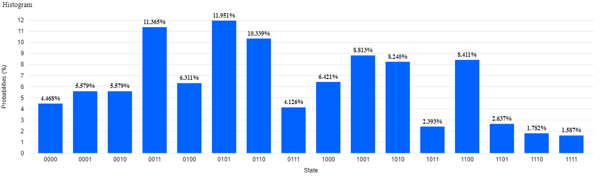
Figure 12: Measurement statistics for $\mathcal{C}_{4,2}$ with $25$ CNOT in transpiled circuit

An $EM$ value of $0$ signifies that the measurement statistics are exactly aligned with the expected ideal results while the $EM$ value can at maximum be $1$. We have calculated the $EM$ values for results of different mappings for the circuit $\mathcal{C}_{4,2}$.

It is very interesting to see that under different mapping of logical qubits to physical qubits in $Q_{1}$ from the user end the IQX mapping solution provided different transpiled circuits. We know that the number of CNOT in $\mathcal{C}_{4,2}$ is $22$. The transpiled circuits for $\mathcal{C}_{4,2}$ had a minimum of $25$ CNOT gates and were as high as $31$ in some cases. The corresponding transpiled circuit contains $25$ CNOT gates which is the least of all the transpiled circuits. Figure 12 shows the measurement statistics corresponding to the circuit with the minimum $EM$ value, which is equal to $0.4088$.

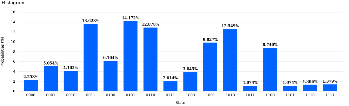
Figure 13: Measurement statistics for $\mathcal{\widehat{C}}_{4,2}$ corresponding to the map $M_{1}$

Next we look at the measurement statistics of the circuit $\mathcal{\widehat{C}}_{4,2}$. There are many mappings between logical and physical qubits in this case such that the CNOT constraint of the circuit is met. Let such a map be $M:\{q_{0},q_{2},q_{3},q_{4}\}\rightarrow\{0,1,2,3,4\}$. Then if there is a CNOT between $q_{i}$ and $q_{j}$ then there is an edge $M(q_{i})\leftrightarrow M(q_{j})$ in graph $G^{Q_{1}}_{A}$. In such mappings the IQX mapping solution didn’t implement any modification in the transpiled circuit as expected.

Here we present the result for the following map $M_{1}$

$$M1:\quad q_{0}\rightarrow 3,\quad q_{1}\rightarrow 2,\quad q_{2}\rightarrow 4,\quad q_{3}\rightarrow 0.$$

Figure 13 shows the measurement statistics corresponding to this mapping and the resultant $EM$ value is $0.282103$. These results show that the circuit $\mathcal{C}_{4,2}$ needs more than the specified number of CNOT while being implemented on “ibmqx2” and the measurement statistics of $\mathcal{\widehat{C}}_{4,2}$ is much more closely aligned with the ideal measurement statistics compared to $\mathcal{C}_{4,2}$.

V-C Modifications leading to different CNOT error distributions

We now discuss how we can in fact use partially defined transformations to further fine tune the circuit $\mathcal{\widehat{C}}_{4,2}$ depending on the specifications of the architecture. We consider a four qubit architecture $A_{4}$ with the same CNOT connectivity as $G^{\mathcal{\widehat{C}}_{4,2}}$ and only differs in CNOT error distribution. We then observe how further modifying the circuit $\mathcal{\widehat{C}}_{4,2}$ can lead to lower CNOT error on expectation against some error distributions in the architecture $A_{4}$. We assume every edge in the CNOT map of $A_{4}$ is bidirectional, as is the case with all currently publicly available IBM-Q machines.

The CNOT error rate when applying a CNOT between qubits $i$ and $j$ (such that the edge $i\leftrightarrow j$ is present in $G_{A}$) is denoted as $e_{ij}$.Figure 15 shows the CNOT map of the architecture.

CNOT error model

In this regard we define our error model to calculate CNOT error on expectation of a circuit implemented in the architecture $A_{4}$. The probability of a CNOT placed between qubits $i$ and $j$ acting erroneously in a circuit is dependent on the error rate of the corresponding CNOT coupling in the architecture. We call this CNOT error. We denote this probability with $f_{e}:[0,1]\rightarrow[0,1]$. We do not assume the exact nature of $f_{e}$, but only that it is directly proportional to error rate (i.e. an increasing function) which is by definition.

Next we define the following Bernoulli random variables to calculate the the number of CNOT acting erroneously on expectation when a circuit is applied on this architecture. We define a variable $x_{k}$ corresponding to each CNOT used in a circuit. The variable is assigned zero if the $k$-th CNOT is applied correctly while executing a circuit, and one otherwise.

Let us suppose the $k$-th CNOT is applied between qubits $i$ and $j$. Then we have $Pr(x_{k}=1)=f_{e}(e_{ij})$ and The expected error while applying the CNOT is $\mathbb{E}(x_{k})=f_{e}(e_{ij})$. Therefore the CNOT error on expectation while implementing a circuit $\mathcal{C}$ on the architecture is

$$\mathbb{E}(\mathcal{C})=\displaystyle\sum v_{ij}f_{e}(e_{ij}).$$

Having described the error model we look at the CNOT distribution of the circuit $\mathcal{\widehat{C}}_{4,2}$ as a weighted graph $G_{f}$. The vertices and the edges of this graph is same as that of $G^{\mathcal{\widehat{C}}_{4,2}}$. The weight of an edge $q_{i}\leftrightarrow q_{j}$ is the number of CNOT gates applied between the two qubits in the circuit. The graph $G_{f}$ is shown in Figure 14.

Now we implement the circuit $\mathcal{\widehat{C}}_{4,2}$ on the architecture $A_{4}$ so that all CNOT constraints can be met. We observe that only the qubit $1$ has degree $3$ and therefore $q_{1}$ is mapped to the physical qubit $1$. Then we can have the following maps which satisfies all the CNOT constraints.

1. $q_{1}\rightarrow 1$, $q_{0}\rightarrow 0$, $q_{2}\rightarrow 2$, $q_{3}\rightarrow 3$.

2. $q_{1}\rightarrow 1$, $q_{0}\rightarrow 2$, $q_{2}\rightarrow 0$, $q_{3}\rightarrow 3$.

Then the expected CNOT error of the circuit $\mathcal{\widehat{C}}_{4,2}$ when applied on the architecture $A_{4}$ is

$$\mathbb{E}(\mathcal{\widehat{C}}_{4,2})=5f_{e}(e_{01})+3f_{e}(e_{02})+3f_{e}(e_{12})+f_{e}(e_{13}).$$

We now show the circuit $\mathcal{\widehat{C}}_{4,2}$ (described in Figure 10) can be further modified using partially defined transformations so that the CNOT error in the circuit on this architecture will reduce on expectation under some error distribution conditions.

Figure 14: Graph $G_{f}$ corresponding to $G^{\mathcal{\widehat{C}}_{4,2}}$.

Figure 15: CNOT map of the architecture $A$.

Figure 16: Graph $G_{f}^{\prime}$ corresponding to $\mathcal{\widehat{C}}_{4,2}^{\prime}$

@C=0.2em @R=1em &