Bound states in semi-Dirac semi-metals

Abstract

New insights into transport properties of nanostructures with a linear dispersion along one direction and a quadratic dispersion along another are obtained by analysing their spectral stability properties under small perturbations. Physically relevant sufficient and necessary conditions to guarantee the existence of discrete eigenvalues are derived under rather general assumptions on external fields. One of the most interesting features of the analysis is the evident spectral instability of the systems in the weakly coupled regime. The rigorous theoretical results are illustrated by numerical experiments and predictions for physical experiments are made.

Semi-Dirac semi-metals have attracted a lot of attention in the last decade; see, e.g., Pardo and Pickett (2009); Banerjee et al. (2009); Delplace and Montambaux (2010); Saha (2016); Banerjee and Narayan and references therein. The most striking feature of these recently discovered nanostructures is that they exhibit unprecedented band structure properties: (electron or hole) quasiparticles disperse linearly in one direction and quadratically in the orthogonal direction. The situation is neither conventional zero-gap semiconductor-like, nor graphene-like, but has in some sense aspects of both.

Using a tight-binding model of spinless fermions, it is commonly accepted that the Hamiltonian

$$H_{0}:=\begin{pmatrix}-i\partial_{y}&-\partial_{x}^{2}+\delta\\ -\partial_{x}^{2}+\delta&i\partial_{y}\end{pmatrix}$$ (1)

is the right low-energy description of the unperturbed system. Here we disregard all the physical constants of Banerjee et al. (2009); Delplace and Montambaux (2010), for they can always be considered to be equal to $1$ by suitably re-scaling the space variables $\bm{r}:=(x,y)\in\mathbb{R}^{2}$, except for the gap parameter $\delta$ which we assume to be a positive constant.

We understand $H_{0}$ as the operator acting in the Hilbert space $\mathcal{H}:=L^{2}(\mathbb{R}^{2})^{2}$ consisting of all $\mathbb{C}^{2}$-valued functions

$$\psi=\begin{pmatrix}\psi_{1}\\ \psi_{2}\end{pmatrix}\qquad\mbox{such that}\qquad\|\psi\|_{\mathcal{H}}^{2}:=\int_{\mathbb{R}^{2}}|\psi|^{2}<\infty\,,$$

where $|\psi|:=\sqrt{|\psi_{1}|^{2}+|\psi_{2}|^{2}}$ is the usual Euclidean norm and $L^{2}(\mathbb{R}^{2})$ is the Lebesgue space of square-integrable functions over $\mathbb{R}^{2}$. For the operator domain, we take

$$\mathop{\mathsf{dom}}H_{0}:=\left\{\psi\in\mathcal{H}:\ \partial_{x}\psi,\,\partial_{x}^{2}\psi,\,\partial_{y}\psi\in\mathcal{H}\right\},$$

which, in contrast to the conventional Dirac operator, is a proper subset of the Sobolev space $H^{1}(\mathbb{R}^{2})^{2}$. Anyway, applying the Fourier transform in the spirit of (Kato, 1966, § V.5.4) or (Thaller, 1992, § 1.4), it is easily verified that $H_{0}$ is self-adjoint and that its spectrum is given by

$$\sigma(H_{0})=(-\infty,-\delta]\cup[\delta,\infty)\,.$$ (2)

Moreover, the total spectrum is purely absolutely continuous, which is traditionally interpreted (see Bruneau et al. for a nice overview) as the existence of transport for the whole set of energies $E$ satisfying $|E|\geq\delta$.

In this paper, we are concerned with spectral stability properties of $H_{0}$. More specifically, we consider a general matrix multiplication operator

$$V:=\begin{pmatrix}V_{11}&V_{12}\\ V_{21}&V_{22}\end{pmatrix},$$ (3)

whose coefficients are bounded complex-valued functions $V_{11},V_{12},V_{21},V_{22}:\mathbb{R}^{2}\to\mathbb{C}$, and study the spectrum of the perturbed operator

$$H_{\varepsilon}:=H_{0}+\varepsilon V\,,\qquad\mathop{\mathsf{dom}}H_{\varepsilon}=\mathop{\mathsf{dom}}H_{0}\,,$$

as the positive coupling parameter $\varepsilon$ tends to zero. To make $H_{\varepsilon}$ self-adjoint, we always assume that $V_{11}$ and $V_{22}$ are in fact real-valued, while $V_{12}$ and $V_{21}$ are allowed to be complex-valued but the Hermiticity relation $V_{21}=\overline{V_{12}}$ is postulated. In addition, we assume that $V_{11},V_{12},V_{22}$ are vanishing at infinity, in order to have (cf. (Thaller, 1992, § 4.3.4)) the stability of the essential spectrum

$$\sigma_{\mathrm{ess}}(H_{\varepsilon})=(-\infty,-\delta]\cup[\delta,\infty)\,.$$ (4)

Recall that the essential spectrum is composed of accumulation points of the spectrum and possibly also of infinitely degenerate eigenvalues. For the stability issues, we are more interested in the discrete spectrum $\sigma_{\mathrm{disc}}(H_{\varepsilon})$, which consists of isolated eigenvalues of finite multiplicities in the essential spectral gap $(-\delta,\delta)$. Physically, the eigenvalues are energies of bound states of $H_{\varepsilon}$ representing stationary solutions of the time-dependent Dirac equation. Our objective is to derive physically relevant sufficient and necessary conditions for the existence of the discrete eigenvalues. Contrary to the Schrödinger case, this is methodologically by no means evident, for no direct variational principles are available for the operator $H_{\varepsilon}$ due to its unboundedness from below.

Our strategy to overcome this difficulty is to pass to the square $H_{\varepsilon}^{2}$, which is a non-negative operator, apply the standard variational principle (see, e.g., (Davies, 1995, § 4.5)) to it and employ the spectral mapping equivalence

$$E\in\sigma(H_{\varepsilon})\quad\Longleftrightarrow\quad E^{2}\in\sigma(H_{\varepsilon}^{2})$$ (5)

valid for all real energies $E$. Consequently, in order to ensure that there exists a discrete eigenvalue $E\in(-\delta,\delta)$, it is enough to construct a test function $\psi\in\mathop{\mathsf{dom}}H_{0}$ such that

$$Q_{\varepsilon}[\psi]:=\|H_{\varepsilon}\psi\|_{\mathcal{H}}^{2}-\delta^{2}\,\|\psi\|_{\mathcal{H}}^{2}<0\,.$$ (6)

Motivated by the theory of quantum waveguides Duclos et al. (2001), we choose the test function as follows. Observing that, formally(!), $H_{0}^{2}\psi^{\pm}\stackrel{{\scriptstyle!}}{{=}}\delta^{2}\psi^{\pm}$, where

$$\psi^{+}:=\begin{pmatrix}1\\ 0\end{pmatrix}\qquad\mbox{and}\qquad\psi^{-}:=\begin{pmatrix}0\\ 1\end{pmatrix},$$ (7)

we see that $\psi^{\pm}$ are generalised eigenvectors of $H_{0}^{2}$ corresponding to the ionisation energy $\delta^{2}$. Therefore they are generalised minimisers of the functional $Q_{0}$ and it is admissible to expect them to be suitable building blocks for possible minimisers of $Q_{\varepsilon}$ as well, at least if $\varepsilon$ is small. Still formally(!), one easily computes

$$Q_{\varepsilon}[\psi^{+}] \!\stackrel{{\scriptstyle!}}{{=}}\!\!\int_{\mathbb{R}^{2}}\!(\varepsilon^{2}|V_{11}|^{2}+\varepsilon^{2}|V_{12}|^{2}+2\delta\varepsilon\,\Re V_{12})=:I_{\varepsilon}^{+},$$ (8)

$$Q_{\varepsilon}[\psi^{-}] \!\stackrel{{\scriptstyle!}}{{=}}\!\!\int_{\mathbb{R}^{2}}\!(\varepsilon^{2}|V_{22}|^{2}+\varepsilon^{2}|V_{12}|^{2}+2\delta\varepsilon\,\Re V_{12})=:I_{\varepsilon}^{-}.$$

To make sense of the integrals, we henceforth assume $V_{11},V_{22}\in L^{2}(\mathbb{R}^{2})$ and $V_{12}\in L^{2}(\mathbb{R}^{2})\cap L^{1}(\mathbb{R}^{2})$. We have thus obtained the following sufficient condition:

$$\left(\,I_{\varepsilon}^{+}<0\quad\mbox{or}\quad I_{\varepsilon}^{-}<0\,\right)\quad\Longrightarrow\quad\sigma_{\mathrm{disc}}(H_{\varepsilon})\not=\varnothing\,,$$ (9)

meaning that $H_{\varepsilon}$ possesses at least one isolated eigenvalue of finite multiplicity located in the interval $(-\delta,\delta)$. As a matter of fact, the variational principle implies that $H_{\varepsilon}$ possesses at least two discrete eigenvalues (counting multiplicities) provided that $I_{\varepsilon}^{+}<0$ and $I_{\varepsilon}^{-}<0$ hold, because the test functions $\psi^{\pm}$ are mutually orthogonal.

To justify the formal computations above ($\psi^{\pm}\not\in\mathcal{H}$ !), we replace the inadmissible test functions (7) by their regularised versions $\psi_{n}^{+}:=\phi_{n}\,\psi^{\pm}$ with $n>1$. Here $\phi_{n}:\mathbb{R}^{2}\to\mathbb{R}$ is a smooth function of compact support such that $\phi_{n}=1$ on the disk of radius $n$, $\phi_{n}=0$ outside the disk of radius $n^{2}$ and $\phi_{n}(\bm{r}):=\xi(f(r))$ elsewhere, where $f(r):=\log_{n}(n^{2}/r)$ with $r:=|\bm{r}|$ and $\xi:\mathbb{R}\to[0,1]$ is any smooth function such that $\xi=0$ in a right neighbourhood of $0$ and $\xi=1$ in a left neighbourhood of $1$. Then the formal results (8) are indeed justified through the limits $Q_{\varepsilon}[\psi_{n}^{\pm}]\to I_{\varepsilon}^{\pm}$ as $n\to\infty$. Consequently, assuming $I_{\varepsilon}^{+}<0$ (respectively, $I_{\varepsilon}^{-}<0$), then there exists a positive number $n_{0}$ such that $Q_{\varepsilon}[\psi_{n}^{+}]<0$ (respectively, $Q_{\varepsilon}[\psi_{n}^{-}]<0$) for all $n>n_{0}$. Hence (9) holds true as well as the remark about the existence of two discrete eigenvalues.

It is remarkable that the sufficient condition (9) is always satisfied in the weakly coupled regime provided that

$$\Re V_{12}<0\,.$$ (10)

Indeed, under this condition, there obviously exists a positive number $\varepsilon_{0}$ such $I_{\varepsilon}^{+}<0$ and $I_{\varepsilon}^{-}<0$ for all $\varepsilon<\varepsilon_{0}$. It follows that, for all sufficiently small $\varepsilon$, $H_{\varepsilon}$ possesses at least two isolated eigenvalues of finite multiplicities located in the interval $(-\delta,\delta)$. We interpret the result as the spectral instability (or criticality) of $H_{0}$, for there always exists an electromagnetic potential $V$ such that the spectrum of $H_{\varepsilon}$ with an arbitrarily small $\varepsilon$ differs from that of $H_{0}$ given by (2).

A special situation in which the discrete spectrum exists is the potential $V$ with vanishing diagonal components $V_{11}=0=V_{22}$ and the off-diagonal component $V_{12}$ satisfying (10). In this case the critical coupling constant satisfies

$$\varepsilon_{0}\geq\frac{-2\delta\,\langle\Re V_{12}\rangle}{\|V_{12}\|^{2}}\,,$$ (11)

where we abbreviate $\langle\Re V_{12}\rangle:=\int_{\mathbb{R}^{2}}\Re V_{12}$ and $\|\cdot\|$ denotes the norm of $L^{2}(\mathbb{R}^{2})$.

At least in this special setting and if $V_{12}$ is real-valued, it is worth noticing that (10) represents also a necessary condition for the existence of discrete spectrum. To see it, let us now assume that $V_{11}=0=V_{22}$ and

$$V_{12}=V_{21}\geq 0\,.$$ (12)

From the first component of the eigenvalue equation $H_{0}\psi=E\psi$, we get $\psi_{2}=-R\,(-i\partial_{y}-E)\psi_{1}$, where the inverse $R:=(-\partial_{x}^{2}+\delta+\varepsilon V_{12})^{-1}$ is a well defined isomorphism on $L^{2}(\mathbb{R}^{2})$ because of (12). Plugging this relationship between $\psi_{1}$ and $\psi_{2}$ into the second component of the eigenvalue equation, we arrive at the functional identity

$$(-\partial_{x}^{2}+\delta+\varepsilon V_{21})\psi_{1}-(i\partial_{y}-E)R(-i\partial_{y}-E)\psi_{1}=0\,.$$

Multiplying both sides by $\overline{\psi_{1}}$, integrating over $\mathbb{R}^{2}$, taking the real part of the obtained scalar identity and using the self-adjointness of $R$, we get

$$\|\partial_{x}\psi_{1}\|^{2}+\delta\,\|\psi_{1}\|^{2}+(\psi_{1},\varepsilon V_{21}\psi_{1})+\|R^{1/2}\partial_{y}\psi_{1}\|^{2}\\ =E^{2}\|R^{1/2}\psi_{1}\|^{2}\,,$$ (13)

where $(\cdot,\cdot)$ denotes the inner product of $L^{2}(\mathbb{R}^{2})$ associated with $\|\cdot\|$. Since $V_{12}$ is assumed to be real-valued, $-\partial_{x}^{2}+\delta+\varepsilon V_{12}(x,y)$ considered as an operator in $L^{2}(\mathbb{R})$ parametrically dependent on $y$ is self-adjoint. Recalling in addition that $V_{12}\geq 0$ vanishes at infinity, so that the spectrum of the one-dimensional Schrödinger operator equals $[\delta,\infty)$, one has the estimate

$$\|R^{1/2}\psi_{1}\|^{2}\leq\|R\|\|\psi_{1}\|^{2}=\delta^{-1}\|\psi_{1}\|^{2}\,.$$

Using this bound in (13), we finally get $\delta^{2}\leq E^{2}$, which proves that the discrete spectrum of $H_{\varepsilon}$ is empty in view of (5) and (4).

Our last theoretical objective is to establish quantitative bounds for the discrete eigenvalues existing under the hypothesis (10) in the weakly coupled regime. To this aim, we henceforth assume that the bounded functions $V_{11},V_{12},V_{22}$ are compactly supported. As in the beginning, we allow $V_{12}$ to be complex-valued. By the variational principle, one has the bound

$$E^{2}-\delta^{2}\leq\frac{Q_{\varepsilon}[\psi_{n}^{\pm}]}{\|\psi_{n}^{\pm}\|_{\mathcal{H}}^{2}}\,,$$

where the test functions $\psi_{n}^{\pm}$ are the regularised versions of (7) as above.

Let us begin with the test function $\psi_{n}^{+}$. One has

$$\|H_{\varepsilon}\psi_{n}^{+}\|_{\mathcal{H}}^{2}$$

$$=\|(-\partial_{x}^{2}+\delta+\varepsilon V_{21})\phi_{n}\|^{2}+\|(-i\partial_{y}+\varepsilon V_{11})\phi_{n}\|^{2}$$

$$=\|\partial_{x}^{2}\phi_{n}\|^{2}+\delta^{2}\|\phi_{n}\|^{2}+2\delta\|\partial_{x}\phi_{n}\|^{2}+\|\partial_{y}\phi_{n}\|^{2}+I_{\varepsilon}^{+}\,,$$

where the second equality holds for all sufficiently large $n$ when $V_{12}$ and $\partial_{x}^{2}\phi_{n}$ (and $V_{11}$ and $\partial_{y}\phi_{n}$) have disjoint supports. Using the chain rule when differentiating $\phi_{n}$, estimating the derivative of $\xi$ by its maximal value $\|\xi^{\prime}\|_{\infty}:=\max_{[0,1]}|\xi^{\prime}|$ and passing to polar coordinates, we have

$$\|\partial_{x}\phi_{n}\|^{2}\leq\frac{\|\xi^{\prime}\|_{\infty}^{2}}{\log^{2}n}\int_{\{n<r<n^{2}\}}\frac{x^{2}}{r^{4}}\,\mathrm{d}x\,\mathrm{d}y=\frac{c_{1}}{\log n}\,,$$

where $c_{1}:=\pi\|\xi^{\prime}\|_{\infty}^{2}$. The same estimate holds for $\|\partial_{y}\phi_{n}\|$. Similarly,

$$\|\partial_{x}^{2}\phi_{n}\|^{2} \leq\frac{2\,\|\xi^{\prime\prime}\|_{\infty}^{2}}{\log^{4}n}\int_{\{n<r<n^{2}\}}\frac{x^{4}}{r^{8}}\,\mathrm{d}x\,\mathrm{d}y$$

$$\quad+\frac{2\,\|\xi^{\prime}\|_{\infty}^{2}}{\log^{2}n}\int_{\{n<r<n^{2}\}}\frac{(x^{2}-y^{2})^{2}}{r^{8}}\,\mathrm{d}x\,\mathrm{d}y$$

$$=\left(\frac{3\pi\|\xi^{\prime\prime}\|_{\infty}^{2}}{4\log^{4}n}+\frac{\pi\|\xi^{\prime}\|_{\infty}^{2}}{\log^{2}n}\right)\left(\frac{1}{n^{2}}-\frac{1}{n^{4}}\right)$$

$$\leq\left(\frac{3\pi\|\xi^{\prime\prime}\|_{\infty}^{2}}{4\log n}+\frac{\pi\|\xi^{\prime}\|_{\infty}^{2}}{\log n}\right)\frac{1}{e^{2}}=:\frac{c_{2}}{\log n}\,,$$

where $e$ is the base of the natural logarithm $\log$ and the last, crude estimate holds for all $n\geq e$.

Using these estimates, we observe that $Q_{\varepsilon}[\psi_{n}^{+}]\to I_{\varepsilon}^{+}$ as $n\to\infty$, in agreement with our claim above. Under the hypothesis (10), the limit $I_{\varepsilon}^{+}$ is negative for all sufficiently small $\varepsilon$; in fact, whenever

$$\varepsilon<\frac{-2\delta\,\langle\Re V_{12}\rangle}{\|V_{11}\|^{2}+\|V_{12}\|^{2}}\,.$$

Henceforth we therefore assume this inequality and then choose $n\geq e$ so large that $Q_{\varepsilon}[\psi_{n}^{+}]$ is negative. Finally, using

$$\|\psi_{n}^{+}\|_{\mathcal{H}}^{2}=\|\phi_{n}\|^{2}\leq\int_{\{r<n^{2}\}}1\,\mathrm{d}x\,\mathrm{d}y=\pi n^{4}\,,$$

it follows that

$$E^{2}-\delta^{2}\leq\frac{1}{\pi n^{4}}\left(\frac{c}{\log n}+I_{\varepsilon}^{+}\right)=:g^{+}(\varepsilon,n)\,,$$

where $c:=c_{1}+2\delta c_{1}+c_{2}$.

Using the test function $\psi_{n}^{-}$ instead of $\psi_{n}^{+}$, the proof follows analogously. In fact, it is enough to replace $V_{11}$ by $V_{22}$ (and thus $I_{\varepsilon}^{+}$ by $I_{\varepsilon}^{-}$) in the formulae above. In particular, we have $E^{2}-\delta^{2}\leq g^{-}(\varepsilon,n)$, where $g^{-}$ is defined as $g^{+}$ with $I_{\varepsilon}^{+}$ being replaced by $I_{\varepsilon}^{-}$.

The function $n\mapsto g^{\pm}(\varepsilon,n)$ achieves its negative minimum for the critical value $n_{\varepsilon}^{\pm}$ satisfying

$$\frac{1}{\log n_{\varepsilon}^{\pm}}:=\frac{-2\,I_{\varepsilon}^{\pm}}{c+\sqrt{c^{2}-cI_{\varepsilon}^{\pm}}}$$

(notice that $n_{\varepsilon}^{\pm}\to\infty$ as $\varepsilon\to 0$). In summary, we have got an explicit quantitative bound for the discrete energies

$$E^{2}-\delta^{2}\leq g^{\pm}(\varepsilon,n_{\varepsilon}^{\pm})\,.$$ (14)

In the weakly coupled regime, one has

$$g^{\pm}(\varepsilon,n_{\varepsilon}^{\pm})\approx-\frac{\delta^{2}\,\langle\Re V_{12}\rangle^{2}\,\varepsilon^{2}}{\pi c}\ \exp\left(\frac{2c}{\delta\,\langle\Re V_{12}\rangle\,\varepsilon}\right)$$ (15)

as $\varepsilon\to 0$.

Now we turn to numerical verifications of the established theoretical results. Our numerical scheme consists in expanding the components $\psi_{1},\psi_{2}$ of an eigenvector $\psi\in\mathop{\mathsf{dom}}H_{0}\subset\mathcal{H}$ of $H_{\varepsilon}$ corresponding to an eigenvalue $E$ into a basis $\{\varphi_{j}\}_{j=1}^{\infty}$ of $L^{2}(\mathbb{R}^{2})$:

$$\psi_{1}=\sum_{j=1}^{\infty}a_{j}\,\varphi_{j}\qquad\mbox{and}\qquad\psi_{2}=\sum_{j=1}^{\infty}b_{j}\,\varphi_{j}\,,$$

where $a_{j}:=(\varphi_{j},\psi_{1})$ and $b_{j}:=(\varphi_{j},\psi_{2})$. The eigenvalue problem $H_{\varepsilon}\psi=E\psi$ in $\mathcal{H}$ is cast into a system of algebraic equations for the coefficients $\bm{a}:=\{a_{j}\}_{j=1}^{\infty}$ and $\bm{b}:=\{b_{j}\}_{j=1}^{\infty}$ in the sequence space $\ell^{2}$:

$$\begin{pmatrix}\bm{C_{11}}&\bm{C_{12}}\\ \bm{C_{21}}&\bm{C_{22}}\end{pmatrix}\begin{pmatrix}\bm{a}\\ \bm{b}\end{pmatrix}=E\begin{pmatrix}\bm{D}&\bm{0}\\ \bm{0}&\bm{D}\end{pmatrix}\begin{pmatrix}\bm{a}\\ \bm{b}\end{pmatrix}\,,$$

where

$$\bm{C_{11}} :=\big{\{}(\varphi_{k},-i\partial_{y}\varphi_{j})+(\varphi_{k},\varepsilon V_{11}\varphi_{j})\big{\}}_{k,j=1}^{\infty}\,,$$

$$\bm{C_{12}} :=\big{\{}(\varphi_{k},(-\partial_{x}^{2}+\delta)\varphi_{j})+(\varphi_{k},\varepsilon V_{12}\varphi_{j})\big{\}}_{k,j=1}^{\infty}\,,$$

$$\bm{C_{21}} :=\big{\{}(\varphi_{k},(-\partial_{x}^{2}+\delta)\varphi_{j})+(\varphi_{k},\varepsilon V_{21}\varphi_{j})\big{\}}_{k,j=1}^{\infty}\,,$$

$$\bm{C_{22}} :=\big{\{}(\varphi_{k},i\partial_{y}\varphi_{j})+(\varphi_{k},\varepsilon V_{22}\varphi_{j})\big{\}}_{k,j=1}^{\infty}\,,$$

$$\bm{D} :=\big{\{}(\varphi_{k},\varphi_{j})\big{\}}_{k,j=1}^{\infty}\,.$$

The numerical approximation consists in replacing the infinite matrices by finite ones. The obtained system can be then solved by standard tools of numerical linear algebra. Since no natural basis seems to be available for the problem, we choose the basis consisting of Gaussian radial basis function centered at a set of scattered nodes, in the line of the Radial Basis Function Method.

In our numerical experiments, we considered potentials $V$ with coefficients being either piecewise-constant or fastly decaying functions. In both cases, we got the same qualitative behaviour of the eigenvalues and a quantitative verification of the spectral enclosure (14). Therefore it is expected that this bound is more universal.

The dependence of several eigenvalues (blue curves) on the coupling parameter $\varepsilon$ in the gap $(-\delta,\delta)$ is depicted in Figure 1 for two seetings. In both cases, $\chi_{D}$ denotes the characteristic function of the disk $D$ of radius $2$ centered at the origin and $\delta=5$. We also plot the bounds $\pm h$ (red curves) of the estimates

$$-h(\varepsilon)\leq E(\varepsilon)\leq h(\varepsilon):=\sqrt{\delta^{2}+g^{\pm}(\varepsilon,n_{\varepsilon}^{\pm})}\,$$ (16)

directly obtained from (14). It turns out that the bounds (16) become too crude for larger values of $\varepsilon$.

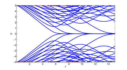
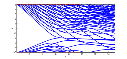
Figure 1: Plots of eigencurves $E(\varepsilon)$ (in blue) and the bounds $h(\varepsilon)$ of (16) (in red) for $\delta=5$. The apparently symmetric setting in the upper figure is due to the choice $V_{11}=0=V_{22}$ and $V_{21}=-\chi_{D}$, while the lower figure corresponds to $V_{21}=-\chi_{D},$ $V_{11}=0.2\chi_{D},$ $V_{22}=-0.9\chi_{D}$.

Figure 2 visualises the ground and excited states.

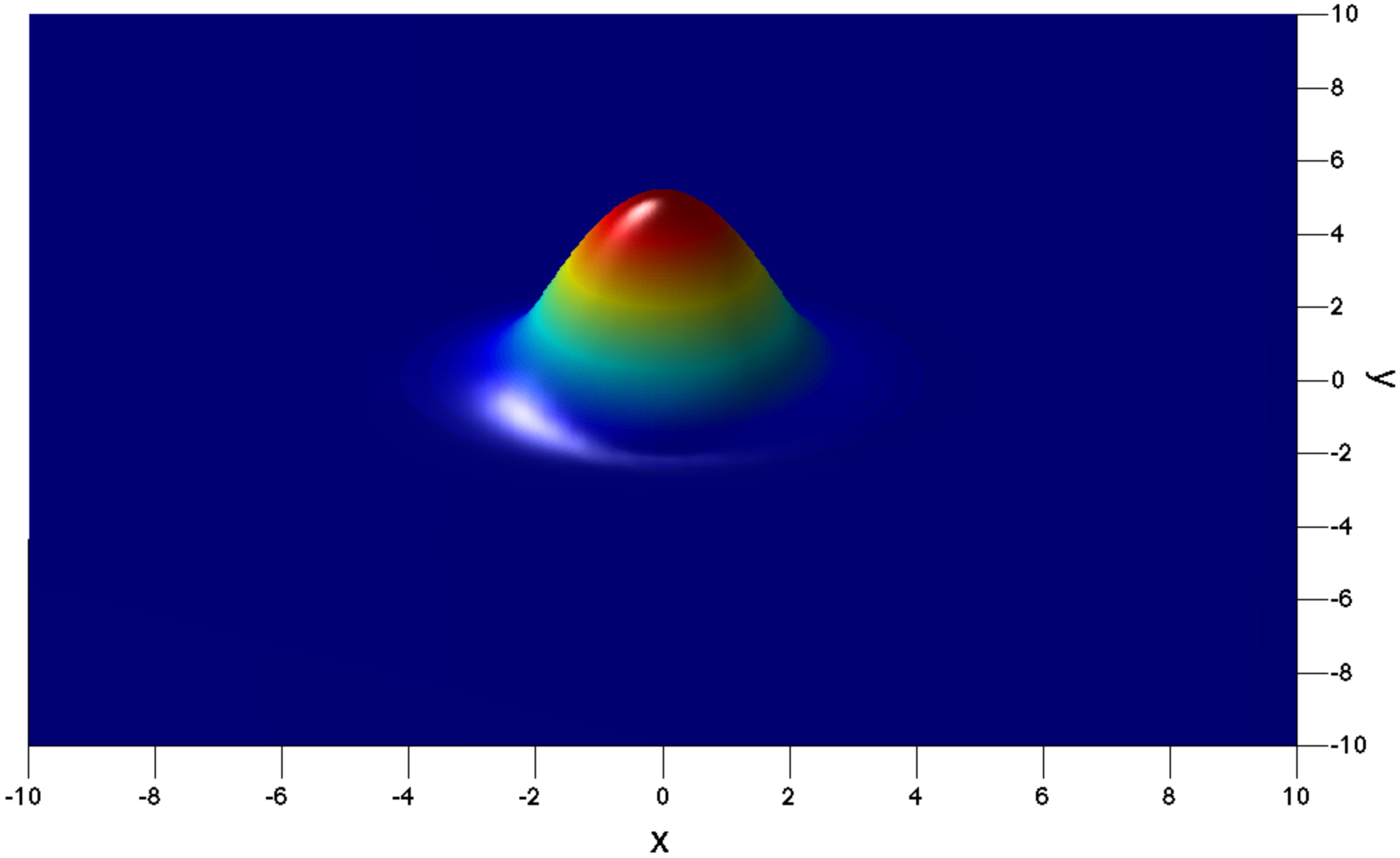
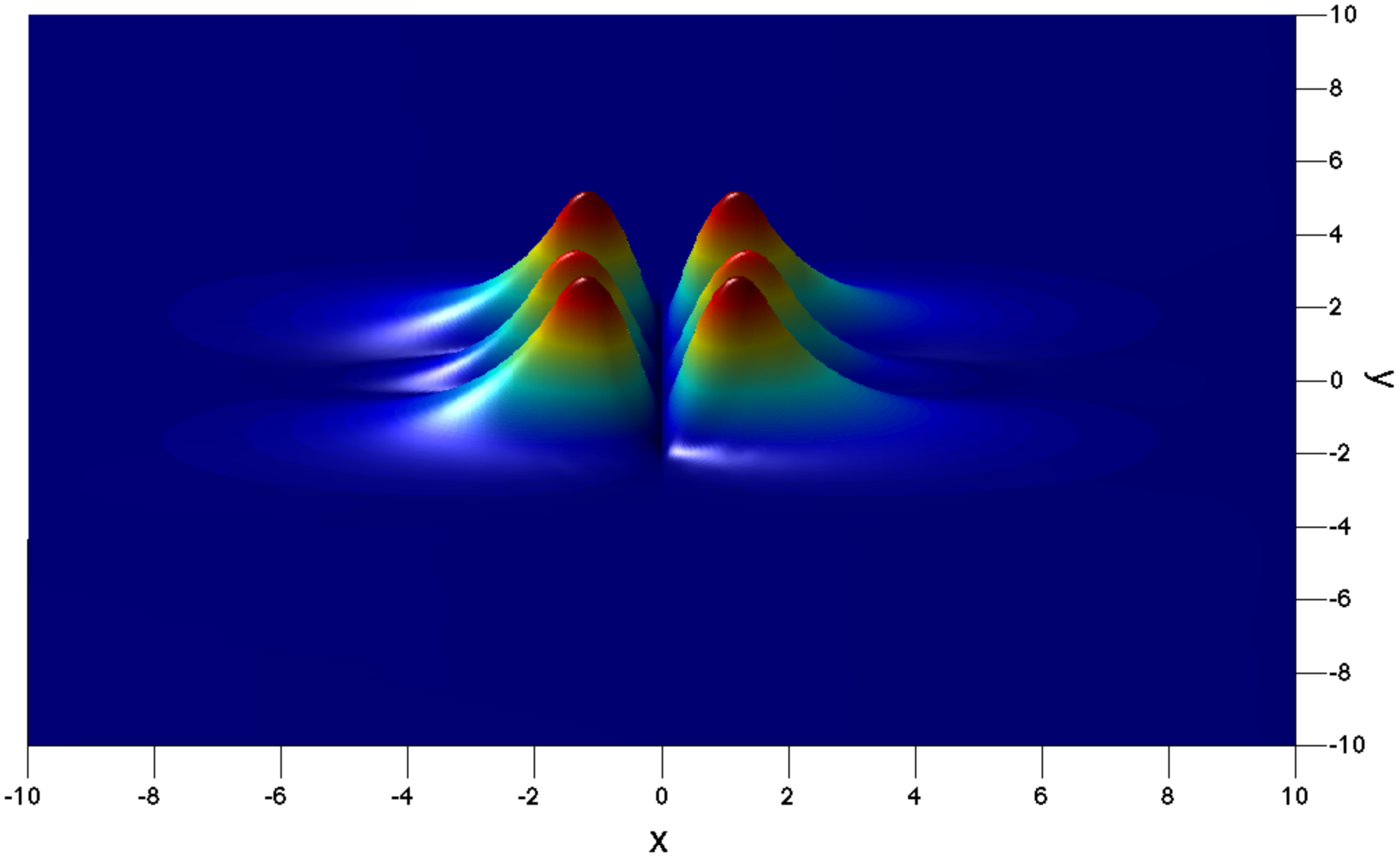
Figure 2: Plots of the magnitude $|\psi|$ of eigenfunctions $\psi$ corresponding to eigenvalues $E\approx 2.9893$ (up) and $E\approx 4.8284$ (down) of the symmetric setting of Figure 1 for $\varepsilon=2.5$.

In conclusion, we have derived sufficient and necessary conditions for the existence of discrete energies in semi-Dirac semi-metals perturbed by general local electromagnetic fields. The existence of bound states is particularly ensured in the regime of weak coupling provided that the off-diagonal component of the perturbation is attractive in the sense of (10). On the other hand, the discrete spectrum is empty in the opposite regime of real-valued repulsive off-diagonal component and absent diagonal components. We have also derived an explicit quantitative bound (14) for the discrete energies. Numerical experiments support our theoretical results and predict the existence of excited states as well.

Because of the tremendous progress in manipulation with materials whose low-energy excitations are described by semi-Dirac fermions, it is our belief that an experimental verification of our theoretical predictions is within the reach of contemporary physics. The simplest experimental setting should be considering an electromagnetic potential (3) with $V_{11}=0=V_{22}$ and $V_{12}=\overline{V_{21}}$ being a locally distributed perturbation (possibly piecewise constant). We predict that the transport properties of the material should significantly depend on the sign of $\Re V_{12}$. Is the estimate (11) on the critical coupling sharp? Do the bound state energies follow the theoretical estimate (14) with (15) in the weakly coupled regime?

The present model is challenging also from purely mathematical perspectives. Because of unavailability of an explicit form of the kernel of the resolvent operator of the unperturbed Hamiltonian $H_{0}$, we have not been able to apply the traditional approach to weakly coupled bound states based on the Birman–Schwinger principle (see the classical reference Simon (1976) in the Schrödinger case). In particular, we leave as an open problem how to establish a (good) lower bound for discrete energies complementing (14), without speaking about the exact asymptotics as $\varepsilon\to 0$. It is also challenging to study perturbations of the non-self-adjoint model recently introduced in Banerjee and Narayan .

This project was partially supported by GAČR grant No. 20-17749X.

References

• Pardo and Pickett (2009) V. Pardo and W. E. Pickett, Phys. Rev. Lett. 102, 166803 (2009).
• Banerjee et al. (2009) S. Banerjee, R. Singh, V. Pardo,  and W. Pickett, Phys. Rev. Lett. 103, 016402 (2009).
• Delplace and Montambaux (2010) P. Delplace and G. Montambaux, Phys. Rev. B 82, 035438 (2010).
• Saha (2016) K. Saha, Phys. Rev. B 94, 081103(R) (2016).
• (5) A. Banerjee and A. Narayan,  arXiv:2001.11188 [cond-mat.mes-hall] (2020).
• Kato (1966) T. Kato, Perturbation Theory for Linear Operators (Springer-Verlag, Berlin, 1966).
• Thaller (1992) B. Thaller, The Dirac equation (Springer-Verlag, Berlin Heidelberg, 1992).
• (8) L. Bruneau, V. Jaksic, Y. Last,  and C.-A. Pillet,  arXiv:1602.01893 [math-ph] (2016).
• Davies (1995) E. B. Davies, Spectral Theory and Differential Operators (Camb. Univ Press, Cambridge, 1995).
• Duclos et al. (2001) P. Duclos, P. Exner,  and D. Krejčiřík, Commun. Math. Phys. 223, 13 (2001).
• Simon (1976) B. Simon, Ann. Phys. 97, 279 (1976).