Noise2Filter: fast, self-supervised learning and real-time reconstruction for 3D Computed Tomography

Abstract

At X-ray beamlines of synchrotron light sources, the achievable time-resolution for 3D tomographic imaging of the interior of an object has been reduced to a fraction of a second, enabling rapidly changing structures to be examined. The associated data acquisition rates require sizable computational resources for reconstruction. Therefore, full 3D reconstruction of the object is usually performed after the scan has completed. Quasi-3D reconstruction — where several interactive 2D slices are computed instead of a 3D volume — has been shown to be significantly more efficient, and can enable the real-time reconstruction and visualization of the interior. However, quasi-3D reconstruction relies on filtered backprojection type algorithms, which are typically sensitive to measurement noise. To overcome this issue, we propose Noise2Filter, a learned filter method that can be trained using only the measured data, and does not require any additional training data. This method combines quasi-3D reconstruction, learned filters, and self-supervised learning to derive a tomographic reconstruction method that can be trained in under a minute and evaluated in real-time. We show limited loss of accuracy compared to training with additional training data, and improved accuracy compared to standard filter-based methods.

¹ Computational imaging group, Centrum Wiskunde & Informatica, Amsterdam 1098 XG, The Netherlands

² Leiden Institute of Advanced Computer Science, Leiden Universiteit, 2333 CA Leiden, The Netherlands

^† Equal contribution.

E-mail: m.j.lagerwerf@cwi.nl

Keywords: Computed Tomography, Reconstruction algorithm, Real-time, Machine learning, Self-supervised learning, Multilayer perceptron, Filtered backprojection, Denoising, Synchrotron

Submitted to: Machine Learning: Science and Technology

1 Introduction

Computed tomography is a non-destructive imaging technique with applications in biology [7], energy research [22], materials science [8], and many other fields [6]. In a tomographic scan, a rotating object is positioned between a source emitting penetrating radiation and a detector that captures the projections of the object. Tomographic reconstruction algorithms compute a 3D image of the interior of the object from its projections. Besides extensive use in medical and laboratory settings, tomography is routinely used at synchrotron facilities, where advances in the last decade have enabled time-resolved imaging of the interior structure of a rapidly changing object [7, 22, 8]. So far, reconstruction algorithms are typically operated offline, enabling visualization of the object only after a scan has completed.

Recent advances in tomographic reconstruction enable real-time interrogation of the reconstructed volume during the scanning process using a quasi-3D reconstruction protocol [2, 3]. In this framework, arbitrarily oriented slices are selected for reconstruction and can be interactively rotated and translated, after which they are reconstructed and visualized virtually instantaneously. This creates the illusion of having access to the full reconstructed 3D volume, but at a fraction of the computational cost. The quasi-3D reconstruction protocol has been implemented in the RECAST3D software package. The information gained from this quasi-3D visualization can be used to directly steer the tomographic experiment, for instance, by adjusting an external parameter — such as temperature — in response to changes in the interior of the object. In addition, the object can be re-positioned, or other acquisition parameters can be adjusted to facilitate the best possible reconstruction [20].

Real-time 3D reconstruction is computationally demanding and data sizes are substantial — data acquisition rates of 7.7GB per second are not uncommon [3]. To attain real-time visualization, the quasi-3D reconstruction protocol is essentially limited to filtered backprojection type methods, since it exploits the locality of backprojection to obtain fast reconstructions. Filtered backprojection (FBP) methods are sensitive to measurement noise, leading to errors in the reconstructed slices [4]. Therefore, application of these methods in the quasi-3D reconstruction protocol is not well-suited to high-noise acquisitions [16, 22], as illustrated in Figure 1.a.

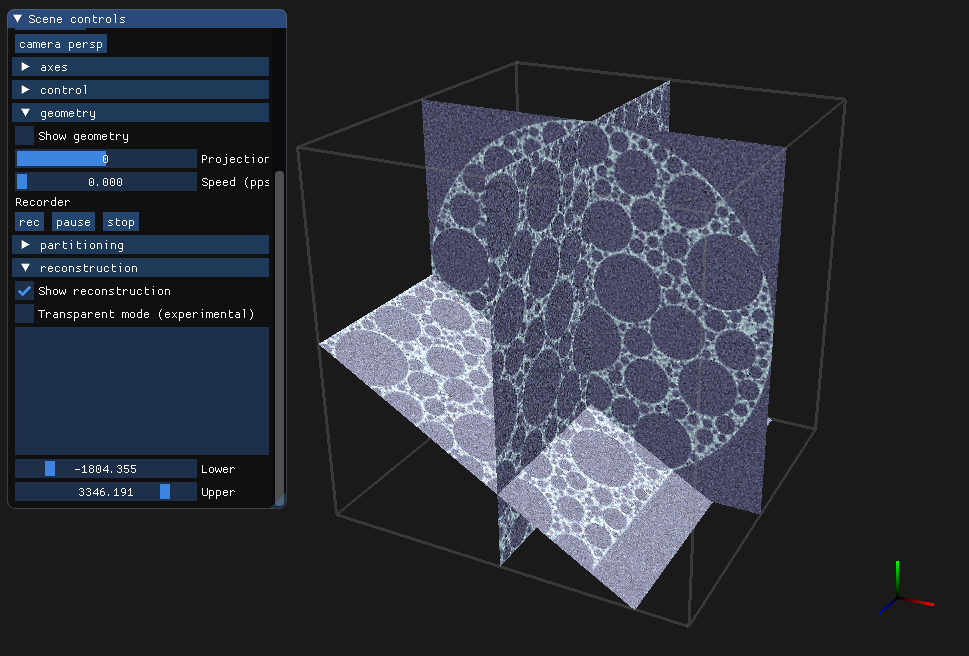
(a) FBP reconstruction

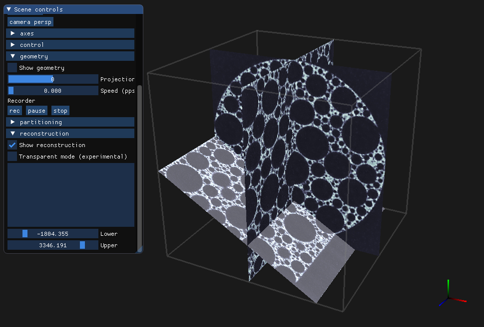
(b) Noise2Filter reconstruction

Figure 1: Real-time reconstructions using FBP and Noise2Filter of a high-noise acquisition using the RECAST3D software package. The highlighted slice is currently being moved.

In this paper, we combine a learning-based filtered reconstruction method with a self-supervised training strategy to obtain Noise2Filter, a denoising FBP-type reconstruction algorithm that can be applied in a quasi-3D reconstruction protocol. This algorithm is designed to be both fast to train and fast to evaluate. Moreover, no additional training data is required other than the measured projection data.

For dynamic scans, our method enables a possible use case where a static scan is performed — with the exact same acquisition rates as the dynamic scan — permitting the Noise2Filter method to be trained immediately. After training for tens of seconds, real-time visualization of the dynamic experiment can ensue, as illustrated in Figure 1.b. In addition, we note that Noise2Filter can be used as a stand-alone reconstruction method.

The first component of our method is the Neural Network filtered backprojection (NN-FBP) method [15]. This method learns a set of filters, along with additional weights, and then forms the reconstructed image as a non-linear function of the individual FBP reconstructions, resulting in higher image quality than standard FBP. However, its application requires the availability of ground truth or high-quality reconstructed images.

This limitation can be overcome using the second component of our method, Noise2Inverse [10], which is a recent machine learning method designed to train denoising convolutional neural networks (CNNs) in inverse problems in imaging. To train a denoising CNN, the method splits the measured projection data to obtain multiple statistically independent reconstructed slices, which are presented to the network during training, without requiring additional high-quality data.

Our main contribution is that we show how to combine the NN-FBP method with the Noise2Inverse training strategy. In addition, we demonstrate that NN-FBP training can be substantially accelerated as compared to previous methods [15]. We evaluate our method on both simulated and experimental datasets, comparing to both conventional filter-based methods and supervised NN-FBP. Finally, we demonstrate that the method can be used in a quasi-3D reconstruction protocol, and exhibit its potential use for dynamic control of tomographic experiments.

The paper is structured as follows. In the next section, we introduce the tomographic reconstruction problem and the filtered backprojection algorithm. In addition, we introduce quasi-3D reconstruction, NN-FBP, and Noise2Inverse. These methods are combined in Section 3, where we describe the Noise2Filter method. In Sections 4 and 5, we describe experiments to analyze the reconstruction accuracy of Noise2Filter on real and simulated CT datasets. Moreover, we study the hyper-parameters of the proposed method. We discuss these results in Section 6.

2 Preliminaries

2.1 Reconstruction problem

In parallel-beam tomography, an unknown object rotates with respect to a planar detector and a parallel source beam. Projections are acquired at a finite number $N_{\text{a}}$ of rotation angles, yielding 2D images defined on an $N\times N$ pixel grid. The reconstruction problem can be modeled by a system of linear equations

$$W\mathbf{x}=\mathbf{y},$$ (1)

where the vector $\mathbf{x}\in\mathbb{R}^{n}$ denotes the unknown object, $\mathbf{y}\in\mathbb{R}^{m}$ describes the measured projection data, and $W=(w_{ij})$ is an $m\times n$ matrix where $w_{ij}$ denotes the contribution of object voxel $j$ to detector pixel $i$. For the sake of simplicity we assume that the volume consists of $n=N\times N\times N$ voxels, and the projection dataset contains $m=N_{\text{a}}\times N\times N$ pixels.

2.2 Filtered backprojection methods

We consider the filtered backprojection (FBP) method for parallel beam tomography [13]. The FBP algorithm is a two step algorithm. First, the data $\mathbf{y}\in\mathbb{R}^{m}$ is convolved over the width of the detector with a one-dimensional filter $\mathbf{h}\in\mathbb{R}^{N_{\text{f}}}$. Next, the backprojection $W^{T}:\mathbb{R}^{m}\rightarrow\mathbb{R}^{n}$ is applied to compute a reconstruction $\mathbf{x}_{\text{FBP}}\in\mathbb{R}^{n}$. Expressing the FBP algorithm in terms of $\mathbf{h}$, $\mathbf{y}$ and $W$ yields

$$\text{FBP}(\mathbf{y},\mathbf{h})=W^{T}(\mathbf{y}\ast\mathbf{h})=\mathbf{x}_{\text{FBP}}.$$ (2)

Observation 1 (FBP is two-step)

The FBP algorithm consists of a filtering step and a backprojection step, and both can be computed separately. That is, the filtering can be performed in advance, and the backprojection can occur on demand. This technique will be used throughout the paper.

We observe that the FBP algorithm can be described by a linear operator when fixing either $\mathbf{y}$ or $\mathbf{h}$. This will be exploited in the discussion of learned filter methods in Section 2.4.

2.3 Quasi-3D reconstruction

A property shared by filtered-backprojection type algorithms is that they are local, in the sense that each voxel of the reconstructed volume can be computed directly from the filtered data by backprojecting onto only that voxel [2]. Therefore, if one is interested in a subset of the reconstructed volume, much of the computational cost of a full 3D reconstruction can be avoided. Specifically, if the reconstructed subset is a rectangular box or a slice, efficient backprojection algorithms such as those implemented in the ASTRA toolbox [18] can be used. This reduces the computational cost of the backprojection step by an order of $N$.

Observation 2 (Locality)

The backprojection operator is local. Computing the backprojection for a single voxel or a subset of voxels is therefore substantially faster than computing the backprojection for all voxels.

This methodology has been implemented in the RECAST3D software package [2], which exposes a limited number of arbitrarily oriented 2D slices. These slices are interactive and can be manipulated by the technician of the tomographic experiment. This technique for real-time visualization has been successfully applied in practice to acquisitions in micro-CT systems [5], synchrotron tomography [3], and electron tomography [20].

2.4 NN-FBP reconstruction algorithm

The NN-FBP algorithm learns a set of suitable filters and a set of weights, and then forms a non-linear model that combines the individual FBP reconstructions. The algorithm may be considered as a multi-layer perceptron [9] that operates pointwise on a collection of suitable reconstructions. A schematic representation of the NN-FBP algorithm is given Figure 2, a mathematical description is given below.

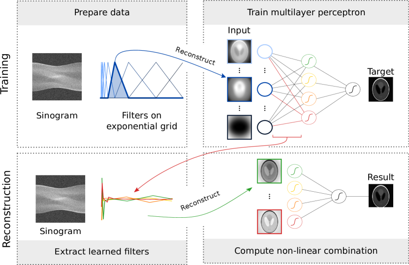
Figure 2: An illustration of the NN-FBP method as applied to a noisy 2D Shepp-Logan sinogram. Before training, the data is reconstructed with filters $\mathbf{e}_{1},\ldots,\mathbf{e}_{N_{e}}$, defined on an exponential grid. These reconstructions $\mathbf{x}_{\mathbf{e}_{1}},\ldots,\mathbf{x}_{\mathbf{e}_{N_{e}}}$ are used as input for training a multilayer perceptron, as described in Equation (5). The training target is a high-quality reconstruction. For reconstruction, learned filters $\mathbf{h}^{1},\ldots,\mathbf{h}^{N_{\text{h}}}$ are extracted from the network (as indicated by the red arrow). Reconstructions are computed using the learned filters, and a non-linear combination is computed, as described in Equation (6).

To obtain these reconstructions, we first make some general observations: a filter $\mathbf{h}$ can be seen as a vector in $\mathbb{R}^{N_{\text{f}}}$, and the FBP method is linear in the filter when fixing the measured projection data $\mathbf{y}$. Therefore, an FBP reconstruction can be expressed as a linear combination in the basis of the filter. Let $\mathbf{e}_{1},\ldots,\mathbf{e}_{N_{\text{f}}}$ be any basis for the space of filters $\mathbb{R}^{N_{\text{f}}}$, such as the standard basis. Define the reconstruction of $\mathbf{y}$ filtered by a basis element $\mathbf{e}_{i}$ as

$$\mathbf{x}_{\mathbf{e}_{i}}:=W^{T}\left(\mathbf{y}\ast\mathbf{e}_{i}\right).$$ (3)

Then we can write the FBP reconstruction as a linear combination of these reconstructions

$$\mathbf{x}_{\text{FBP}}(\mathbf{y},\mathbf{h}) =\sum_{i=1}^{N_{\text{f}}}\mathbf{h}_{i}\mathbf{x}_{\mathbf{e}_{i}}=\sum_{i=1}^{N_{\text{f}}}W^{T}\left(\mathbf{y}\ast\mathbf{h}_{i}\mathbf{e}_{i}\right)=W^{T}\left(\mathbf{y}\ast\mathbf{h}\right),$$ (4)

where $\mathbf{h}_{i}$ denotes the coordinate of the $i$th basis element $\mathbf{e}_{i}$.

Given a set of $N_{\text{h}}$ filters $\mathbf{h}^{1},\ldots,\mathbf{h}^{N_{\text{h}}}$, we can define a multi-layer perceptron (MLP) with one hidden layer as a function of the reconstructions $\mathbf{x}_{\mathbf{e}_{1}},\ldots,\mathbf{x}_{\mathbf{e}_{N_{\text{f}}}}$

$$\text{MLP}_{\theta}(\mathbf{x}_{\mathbf{e}_{1}},\ldots,\mathbf{x}_{\mathbf{e}_{N_{\text{f}}}}) =\sigma\left(\sum_{k=1}^{N_{\text{h}}}\mathbf{a}_{k}\sigma\left(\sum_{i=1}^{N_{\text{f}}}\mathbf{h}_{i}^{k}\mathbf{x}_{\mathbf{e}_{i}}-\mathbf{b}_{k}\right)-\mathbf{b}_{0}\right),$$ (5)

where $\sigma$ is a non-linear activation function, such as the sigmoid. The multi-layer perceptron has free parameters $\theta=(\mathbf{a},\mathbf{b},\mathbf{h}^{1},\ldots,\mathbf{h}^{N_{\text{h}}})$. Plugging Equation (4) into Equation (5), we obtain the NN-FBP reconstruction algorithm

$$\text{NN-FBP}_{\theta}(\mathbf{y}) =\sigma\left(\sum_{k=1}^{N_{\text{h}}}\mathbf{a}_{k}\sigma\left(\text{FBP}(\mathbf{y},\mathbf{h}^{k})-\mathbf{b}_{k}\right)-\mathbf{b}_{0}\right),$$ (6)

which is amenable to fast, parallel computation because it is a non-linear combination of FBP reconstructions.

Observation 3 (pointwise)

Note that the multi-layer perceptron operates point-wise on the voxels of the reconstructed volumes. Therefore, a single voxel can be computed without having to reconstruct other voxels. This observation connects to the observation of locality on Page 2, and will return several times in this paper.

Supervised training [9] is used to determine the free parameters of the MLP defined in Equation (5). The goal is to approximate a suitable target reconstruction $\mathbf{x}_{\text{Target}}$ by minimizing

$$\left\|\text{MLP}_{\theta}(\mathbf{x}_{\mathbf{e}_{1}},\ldots,\mathbf{x}_{\mathbf{e}_{N_{\text{f}}}})-\mathbf{x}_{\text{Target}}\right\|_{2}^{2},$$ (7)

i.e., the mean square error with respect to the target reconstruction.

The size of the training problem in Equation (7) is related to the number of reconstructed volumes $\mathbf{x}_{\mathbf{e}_{1}},\ldots,\mathbf{x}_{\mathbf{e}_{N_{\text{f}}}}$ and the size of these reconstructions, which suggests two techniques that may be used to accelerate training. First, to reduce the number of reconstructions, the filter is expressed on an exponentially binned grid, which grows logarithmically in the width of the filter. Since the filter width is proportional to the number of pixels in each detector row, we have $N_{e}=O(\log N_{\text{f}})=O(\log N)$. This technique yields suitable filter approximations, as observed in [15, 12]. Second, training may be accelerated by sampling a subset of voxels on which to minimize Equation (7), rather than the full volume. Subsampling is possible because NN-FBP operates pointwise, as noted in Observation 3.

To summarize, we can split the NN-FBP algorithm into three parts, namely: (1) data preparation, where the input training data $\mathbf{x}_{\mathbf{e}_{1}},\ldots,\mathbf{x}_{\mathbf{e}_{N_{e}}}$ is computed, (2) network training, where the weights $\theta^{\star}$ for the network are determined using a supervised learning approach, and (3) the reconstruction algorithm, which is summarized in Algorithm 1.

Algorithm 1 NN-FBP reconstruction algorithm

1:  Given projections $\mathbf{y}$ and a set of parameters $\theta^{\star}~{}:=~{}\left(\mathbf{a},\mathbf{b},\mathbf{h}^{1},\ldots,\mathbf{h}^{N_{\text{h}}}\right)$.

2:  Compute the FBP reconstruction using the learned filters:

3:  for $k=\{1,2,..,N_{h}\}$ do

4:     $\mathbf{x}_{\mathbf{h}^{k}}=\text{FBP}(\mathbf{y},\mathbf{h}^{k})$

5:  end for

6:  Compute a non-linear combination of these reconstructions:$\text{NN-FBP}_{\theta^{\star}}(\mathbf{y})=\sigma\left(\sum_{k=1}^{N_{\text{h}}}\mathbf{a}_{k}\sigma\left(\mathbf{x}_{\mathbf{h}^{k}}-\mathbf{b}_{k}\right)-\mathbf{b}_{0}\right)$

2.5 Noise2Inverse training

Noise2inverse is a technique to train a convolutional neural network (CNN) to denoise reconstructed images in a self-supervised manner [10]. This means that no additional training data is required beyond the acquired noisy measurements. The key idea is change the training strategy by splitting the projection dataset into subsets, computing sub-reconstructions with these subsets and train a neural network mapping one sub-reconstruction to another.

First, the projection data is split into $N_{\text{s}}$ sub-datasets such that projection images from successive angles are placed in different sub-datasets $\mathbf{y}_{1},\mathbf{y}_{2},\ldots,\mathbf{y}_{N_{\text{s}}}$. The network is trained to predict the reconstruction from one subset using the reconstruction of the other subsets. Training therefore aims to find the parameter $\theta^{\star}$ that minimizes

$$\sum_{j=1}^{N_{\text{s}}}\left\|\mathrm{CNN}_{\theta}(\text{FBP}(\mathbf{y}_{j}))-\text{FBP}(\mathbf{y}_{l\neq j})\right\|_{2}^{2},$$ (8)

where $\text{FBP}(\mathbf{y}_{j})$ denotes the reconstruction from one subset of the data, and $\text{FBP}(\mathbf{y}_{l\neq j})$ denotes the FBP reconstruction of the remaining subsets. We observe that the FBP reconstruction of a projection dataset is the mean of the FBP reconstruction of each projection image individually, which enables us to obtain

$$\text{FBP}(\mathbf{y}_{l\neq j})=\frac{1}{N_{\text{s}}-1}\sum_{l\neq j}\text{FBP}(\mathbf{y}_{l}).$$ (9)

Now the original training data can be denoised by applying the trained network to each subreconstruction individually and averaging to obtain

$$\mathbf{x}_{\text{N2I}}=\frac{1}{N_{\text{s}}}\sum_{i=1}^{N_{\text{s}}}\mathrm{CNN}_{\theta^{\star}}(\text{FBP}(\mathbf{y}_{i})).$$ (10)

In the previous discussion, we have assumed that the target images are reconstructed from more subsets than the input images. As in [10], we call this the 1:X strategy. A reverse X:1 training strategy is also possible. Here, the target is a single subreconstruction and the input is reconstructed from the remaining sub-datasets.

Note that convolutional neural networks take into account the surrounding structure of a voxel, typically a 2D slice, and thus do not operate pointwise. Therefore, these networks are are an example where Observation 3 does not apply.

3 Noise2Filter method

Our proposed method combines the three ideas introduced in the previous section. The NN-FBP method is trained on a single projection dataset using the Noise2Inverse training strategy. This enables fast reconstruction of arbitrarily oriented slices using the NN-FBP reconstruction algorithm in a quasi-3D reconstruction protocol.

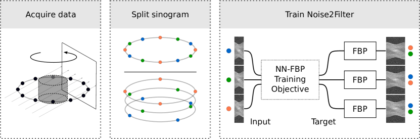
Figure 3: An illustration of the training of the Noise2Filter method. Data is acquired using a 3D parallel beam geometry. For each detector row, the sinogram is split in three sub-datasets such that acquisitions from successive projection angles belong to different sub-datasets. Each sub-dataset is used as input for NN-FBP training; the remaining sub-datasets are used in the target FBP reconstruction. This illustration depicts the 1:X strategy. In the X:1 strategy, the input is computed from the majority of the data, and the target from the minority, rather than vice versa.

Training The training procedure for the Noise2Filter method is similar to the NN-FBP procedure described in [15], with two notable exceptions. First, instead of minimizing the supervised training objective in Equation (7), Noise2Filter minimizes a self-supervised training objective similar to Equation (8). Second, training voxels are sampled from a subset of the reconstructed volume, rather than the full volume.

As in Noise2Inverse, the projection data $\mathbf{y}$ is split into $N_{\text{s}}$ subdatasets with FBP reconstructions $\mathbf{x}_{\text{FBP},j},j=1,\ldots,N_{\text{s}}$. For each subdataset $\mathbf{y}_{j}$, we denote with $\mathbf{x}_{j,\mathbf{e}_{i}}$ a reconstruction filtered with basis element $\mathbf{e}_{i}$.

Training aims to minimize the difference between the MLP output of a subset of projection data and the FBP reconstruction of the remaining data. For the 1:X training strategy, the MLP operates on a single subset of the data and the target is reconstructed from the remaining subsets. For the X:1 training strategy, on the other hand, the target is reconstructed from a single subdataset, and the MLP operates on the remaining subsets. The self-supervised training objective thus becomes:

$$\sum_{j=1}^{N_{\text{s}}}\left\|\text{MLP}_{\theta}(\mathbf{x}_{j,\mathbf{e}_{1}},\ldots,\mathbf{x}_{j,\mathbf{e}_{N_{e}}})-\mathbf{x}_{\text{FBP},l\neq{}j}\right\|_{2}^{2}, \quad(\text{\bf X:1 strategy})$$ (11)

$$\sum_{j=1}^{N_{\text{s}}}\left\|\text{MLP}_{\theta}(\mathbf{x}_{l\neq j,\mathbf{e}_{1}},\ldots,\mathbf{x}_{l\neq j,\mathbf{e}_{N_{e}}})-\mathbf{x}_{\text{FBP},j}\right\|^{2}_{2}, \quad(\text{\bf 1:X strategy})$$ (12)

with

$$\mathbf{x}_{\text{FBP},l\neq{}j}=\frac{1}{N_{\text{s}}-1}\sum_{l\neq j}\mathbf{x}_{\text{FBP},l},\quad\mathbf{x}_{l\neq j,\mathbf{e}_{i}}=\frac{1}{N_{\text{s}}-1}\sum_{l\neq j}\mathbf{x}_{l,\mathbf{e}_{i}}.$$ (13)

A schematic summary of the 1:X training strategy is given in Figure 3.

The second difference is related to the voxels that are considered for the training. Like NN-FBP, we minimize the training objective on a random sample of $N_{\text{T}}$ voxels. We have $N_{\text{T}}\ll N^{3}$, and increasing the sample size in response to increasing object size has been observed to yield diminishing returns. Unlike NN-FBP, training voxels are sampled only from the reconstructions of the axial, frontal, and longitudinal ortho-slices, rather than the full volume. This choice substantially reduces the computational effort of the data preparation step, as shown below.

Data preparation We discuss the 1:X strategy; similar statements hold true for the X:1 strategy.

The data preparation step is the most computationally expensive part of the method. In this step, an input reconstruction $\mathbf{x}_{l\neq j,\mathbf{e}_{i}}$ is computed for each subdataset $\mathbf{y}_{j}$ and each basis element $\mathbf{e}_{i}$. In addition, a target reconstruction $\mathbf{x}_{\text{FBP},j}$ is computed for each subdataset, resulting in a total of $N_{\text{s}}(N_{e}+1)$ reconstructions. These reconstructions are computed on the ortho-slices instead of the full volume. Due to locality — see Observation 2 — the computational cost of the data preparation is therefore reduced by an order of $N$.

Note that the computational cost of the FBP algorithm scales linearly in the number of projection angles, therefore the computational cost of this step is equal to $3(N_{e}+1)$ FBP reconstructions of a 2D slice. Splitting the projection data thus has no adverse effect on the performance.

Reconstruction The reconstruction algorithm is almost identical to the NN-FBP reconstruction algorithm described in Algorithm 1. Whereas the aim of NN-FBP is to reconstruct the full volume, we aim only to reconstruct slices on demand. Therefore, reconstruction can be substantially accelerated.

We make use of Observation 1 that the FBP algorithm can be split in a filtering and backprojection step. First, the acquired projection data is filtered with the learned filters and cached. Then, a single slice can be reconstructed using Algorithm 1, which can occur in real-time due to the locality of the backprojection (Observation 2) and the pointwise nature of the multi-layer perceptron (Observation 3). Therefore, the reconstruction can be integrated in the quasi-3D reconstruction protocol, computing reconstructions of arbitrarily oriented slices in real time.

We note that the reconstruction step deviates slightly from the Noise2Inverse reconstruction described in Equation (10). Rather than averaging separate reconstructions of each subset of the projection data, Noise2Filter computes a reconstruction using the learned filters directly from all data. In the context of self-supervised learning, this technique has been observed to yield improved results [1].

Noise2Filter summary

The Noise2Filter method consists of three steps. A summary of these steps, and specifically the computations performed, is given below:

1. Data preparation Compute the input and target training pairs from the measured projection data $\mathbf{y}$. Specifically, split the measured projection data in $N_{\text{s}}$ equal sub-datasets and compute the following for the ortho-slices:

   $$\text{FBP}(\mathbf{y}_{i},\mathbf{h}) \text{ for }i=1,\ldots,N_{\text{s}}$$ (14)

   $$\text{FBP}(\mathbf{y}_{i},\mathbf{e}_{j}) \text{ for }i=1,\ldots,N_{\text{s}},j=1,\ldots,N_{e}.$$ (15)

   The computational effort of this step is equal to $3(N_{e}+1)$ FBP reconstructions of a 2D slice.

2. Training Obtain a random sample of $N_{\text{T}}$ voxels on the ortho-slices for inclusion in the training set. Compute the optimal parameters $\theta^{\star}$ that minimizes the training objective with respect to the sampled voxels. Note that the training time depends on the size of the training set, which may be fixed independent of the object size.

3. Reconstruction Using the computed parameters $\theta^{\star}$, compute an NN-FBP reconstruction for the desired 2D slices. Recall from Equation (6) that the computational cost of an NN-FBP reconstruction is equivalent to $N_{\text{h}}$ FBP reconstructions.

4 Experimental setup

In this section we discuss the setup of the experiments. Specifically, we describe the data used in the experiments, the implementation of NN-FBP and Noise2Filter, and the measures used to quantify these comparisons.

4.1 Simulated data

A phantom was generated by removing 100,000 randomly-placed non-overlapping balls from a foam cylinder. The foam_ct_phantom package [16] was used to generate analytical projection images with $2\times$ supersampling, were each pixel’s value is averaged over four equally-spaced rays through the pixel. The result contains $1024$ equally-spaced projection images with $512\times 768$ pixels.

In each experiment, the simulated projection images were corrupted with Poisson noise of various levels of intensity, by altering the incident photon count per pixel $I_{0}$. The average absorption of the sample was $10\%$. Reconstructions without Poisson noise and with Poisson noise ($I_{0}=1000$) are shown in Figure 5.

4.2 NN-FBP and Noise2Filter

Noise2Filter and NN-FBP benefit from a shared implementation. Therefore, most almost all implementation details are the same. As in the original NN-FBP implementation [15], the number of learned filters is set to $N_{\text{h}}=4$, the non-linear activation function is the sigmoid, the exponential binning parameter is set to $2$, but the filters are piece-wise linear — rather than piece-wise constant — as proposed in [12]. Moreover, changes have been made to the shared implementation in order to accelerate data preparation, training, and reconstruction.

In the data preparation step, reconstructions are computed of the ortho-slices rather than the full volume. These reconstructions are performed using the RECAST3D software package [2].

Some changes have been made to the training procedure. As in the original implementation, the training objective is minimized using the Levenberg-Marquadt algorithm (LMA), which requires that the data samples are split into a training set and a validation set. Compared to the original implementation, however, the number of training samples is reduced from $10^{6}$ to $5\cdot 10^{4}$. The effect of this reduction is discussed in Section 5.2. In addition, training is accelerated by performing computations on the graphics processing unit (GPU) using PyTorch [14].

Final reconstructions are computed using the RECAST3D software package [2].

NN-FBP The free parameters for the NN-FBP method are trained and tested on separate tomographic datasets. The training dataset consists of paired noisy and noiseless reconstructions. Supervised training minimizes the training objective in Equation (7).

Noise2Filter The Noise2Filter parameters are optimized using self-supervised training on the noisy test dataset, rather than on a separate training dataset. No noiseless reconstructions are necessary for training. Depending on the training strategy (X:1 or 1:X), training minimizes either Equation (11) or (12).

4.3 Quantitative measures

Reconstruction accuracy is quantified using the the Peak Signal-to-Noise Ratio (PSNR) and the Structural Similarity (SSIM) index [21] metrics. Both metrics were computed with respect to the noiseless reconstructed images and using a data range that was determined by the minimum and maximum intensity of the noiseless reconstructed images. If not otherwise mentioned, the reported metrics are the average of the metric as computed on the three ortho-slices.

5 Experiments & Results

We performed several experiments to evaluate the Noise2Filter method. We provide a short summary below.

Reconstruction accuracy We compare Noise2Filter to supervised NN-FBP training and several standard FBP improvement strategies in terms of reconstruction accuracy.

Hyperparameter analysis Implementation choices in the design of the Noise2Filter method are analyzed, including the number of training samples, training strategy (X:1 or 1:X), and number of splits.

Timing An analysis of data preparation and reconstruction speed is given.

Experimental data The method is applied to experimental data, including a showcase that illustrates the potential for use in dynamic control.

5.1 Reconstruction accuracy comparison

In this section, we assess the reconstruction accuracy of the Noise2Filter method. We compare to other filter-based reconstruction techniques in terms of reconstruction accuracy. Specifically, we compare to a baseline FBP reconstruction (with a Ram-Lak filter) and FBP with standard noise reduction techniques — Gaussian filtering (FBP_G) and frequency scaling (FBP_sc). These two methods are discussed in more detail in Appendix A. In addition, we compare to the NN-FBP, which is trained on a separate training dataset with ground truth images.

The comparison is performed on the simulated foam dataset with varying levels of Poisson noise. The incident photon count $I_{0}$ was varied between $1000$ and $32,000$ in powers of two.

For each of the methods, parameter selection was performed as follows. For Noise2Filter, training was performed on the noisy test set. For NN-FBP, training was performed on a separate training dataset. For both methods, training was repeated 20 times to obtain statistics for the PSNR and SSIM. For Gaussian filtering and frequency scaling, the parameters maximizing the SSIM on the test set were determined using a linear grid search.

The Noise2Filter method with the 1:X training strategy and $3$ splits is used. We find that this yields consistent results at various noise levels.

The quantitative measures for the ortho-slices are shown in Figure 4. For all noise levels, the Noise2Filter metrics are higher than FBP with frequency scaling or Gaussian filtering. The NN-FBP method attains the best metrics, although the difference with Noise2Filter decreases as the noise level decreases. The difference in reconstruction accuracy is illustrated in Figure 5, where the ground truth phantom and reconstructions for all considered methods are shown for the incident photon count $I_{0}=1000$. Notice that NN-FBP and Noise2Filter remove the noise in the voids, unlike the FBP methods.

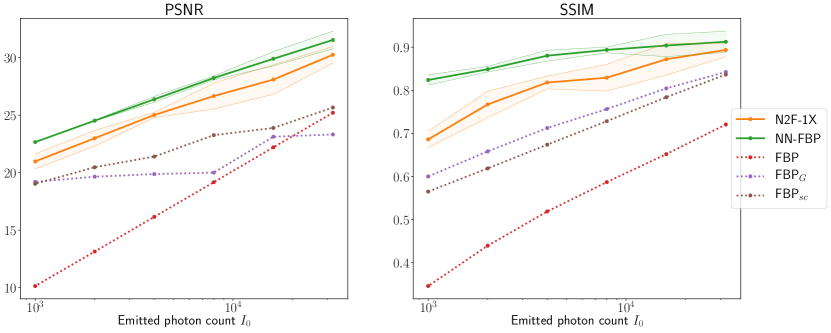
Figure 4: Reconstruction accuracy comparison of Noise2Filter (N2F-1X), NN-FBP, and FBP with Gaussian filtering, frequency scaling, and default filter. For varying noise levels, the average (line) and standard deviation (shaded region) over 20 trials of the PSNR and SSIM are reported. 

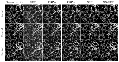
Figure 5: Results of noiseless reconstruction, FBP reconstruction, FBP with frequency scaling ($\text{FBP}_{sc}$), FBP with Gaussian filtering ($\text{FBP}_{G}$), Noise2Filter (N2F), and NN-FBP on a simulated foam phantom with photon count $I_{0}=1000$. Results are shown on an axial, frontal, and $45^{\circ}$ slanted slice. The insets are zoomed by a factor of four.

5.2 Hyper parameter analysis

We consider three hyper parameters for the N2F method: the number of samples considered for training, the training strategy X:1 or 1:X and the number of splits $N_{\text{s}}$ for the measured projection data.

First, we analyzed the reconstruction accuracy as a function of $N_{\text{T}}$, the number of training samples used in the training process. Here, the number of validation samples is fixed to $10\%$ of the number of training samples. Noise was applied to the projection dataset equivalent to $I_{0}=1000$. The results for this experiment are shown in Figure 6. We observe that increasing the number of voxels yields virtually no increase in PSNR or SSIM beyond $N_{\text{T}}=5\cdot 10^{4}$ voxels.

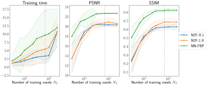
Figure 6: Training time and reconstruction accuracy for varying amounts of training voxels $N_{\text{T}}$. The mean (line) and standard deviation (shaded region) over 50 trials are reported. For both NN-FBP and Noise2Filter, increasing $N_{\text{T}}$ yields diminishing returns in terms of PSNR and SSIM beyond $N_{\text{T}}=5\cdot 10^{4}$, as indicated by the dashed line. 

Second, we compare the training strategies and the number of splits on the simulated foam dataset for two noise levels, $I_{0}=1000$ and $I_{0}=8000$. For various values of the number of splits, 20 networks were trained and used to reconstruct the projection data. The average and standard deviation of the PSNR and SSIM are shown in Figure 7. For both noise levels we observe that the 1:X strategy with $3$ splits obtains the best SSIM and close to the best PSNR.

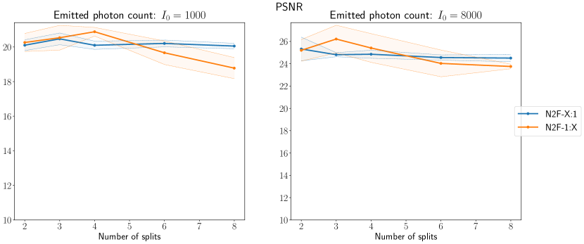
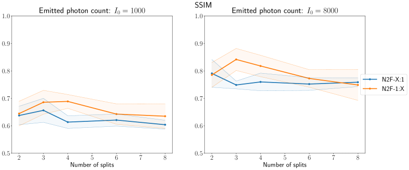
Figure 7: A comparison of Noise2Filter reconstruction accuracy for varying number of splits $N_{\text{s}}$ and training strategies X:1 and 1:X. Mean (line) and standard deviation (shaded region) over 20 trials of the PSNR and SSIM are plotted for noise levels $I_{0}=1000$, and $I_{0}=8000$. 

5.3 Timing comparison

We give timings for the data preparation and training step of the Noise2Filter method for several problem sizes. The computations were performed on a server with 375 GB of RAM and made use of a single Nvidia GeForce RTX 2080 Ti GPU (Nvidia, Santa Clara, CA, USA).

In Table 1 we report the reconstruction times of one 2D slice using the RECAST3D framework for standard FBP and the Noise2Filter method. We see that Noise2Filter is roughly 4 times slower than standard FBP, which is expected considering that we use $N_{\text{h}}=4$ learned filters.

Data size				Duration (seconds)
# voxels	# pixels	# angles	$N_{e}$	DP	FBP	N2F
$128^{3}$	$128\times 192$	256	10	0.34	$0.003$	$0.009$
$256^{3}$	$256\times 384$	512	11	1.34	$0.006$	$0.024$
$512^{3}$	$512\times 768$	1024	12	6.08	$0.030$	$0.114$
$1024^{3}$	$1024\times 1536$	2048	13	44.00	—	—

Table 1: Benchmark results for the data preparation (DP) and reconstruction steps. FBP and Noise2Filter (N2F) reconstructions are performed on a single slice from filtered projection data. Due to memory constraints, some reconstructions not be performed, as indicated by a —.

5.4 TomoBank dynamic dataset

We consider two experiments with an experimental dynamic tomographic dataset, consisting of $60$ scans at consecutive time steps. First, we train Noise2Filter on the data from the first time step and use the trained reconstruction method to compute reconstructions for later time steps. This experiment aims to reveal the ability of Noise2Filter to generalize over dynamics in time. Second, we consider determining the correct center of rotation using Noise2Filter.

The experimental data is taken from the public TomoBank repository [6] and was acquired at the TOMCAT beamline at the Swiss Light Source (Paul Scherrer Institut, Switzerland). In this experiment, sub-second X-ray tomographic microscopy was used to investigate liquid water dynamics in a fuel cell during operation. The experiment took less than 6 seconds, during which 60 scans were acquired. A scan consists of 301 projections taken by a detector with $1100\times 1440$ detector pixels.

First, we train a Noise2Filter network at the first time step $T=0$ and use this network to evaluate all further time steps. Figure 8 shows the results for this strategy for $T=0,19,39,59$ and the FBP reconstructions at these time steps. There is no visible deterioration of the reconstruction accuracy over time, indicating that the trained network generalizes over the whole experiment.

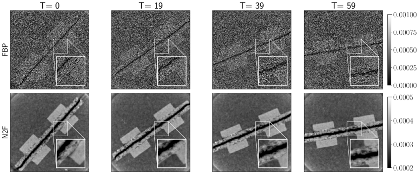
Figure 8: Reconstruction of the fuel cell at various time steps using FBP and Noise2Filter (N2F). The Noise2Filter method was trained on the first time step and also used to reconstruct later time steps. The insets are zoomed by a factor two.

Second, we consider determining the correct center of rotation. In the presence of noise, determining the correct center of rotation for a dataset can be difficult and is often performed after acquiring the measured projection data. Using the tools developed in [20], the center of rotation can be adapted interactively in real-time. In Figure 9 we show Noise2Filter and FBP reconstructions with shifted centers of rotation at the first time step. We note that no retraining was performed for Noise2Filter: the network parameters were determined once using a shift of $0$ pixels. In the FBP reconstructions, the center of rotation artifacts (half moons) are difficult to discern. In the Noise2Filter reconstruction, however, these artifacts are both clearly visible, and visibly disappear at a shift of $19$ pixels, which coincides with the reported center of rotation in [6].

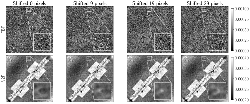
Figure 9: Reconstructions of a fuel cell at various centers of rotation using FBP and Noise2Filter (N2F). In the inset, a center of rotation artifact is highlighted, which disappears at a shift of $19$ pixels. The contrast in the Noise2Filter reconstruction is increased. The insets are zoomed by a factor four.

6 Conclusion

We have introduced Noise2Filter, a machine learning method for denoising filter-based reconstruction that does not require any additional training data beyond the acquired measurements. We show that this self-supervised method improves reconstruction accuracy compared to standard filter-based methods, and has limited loss of accuracy compared to its supervised counterpart (NN-FBP). The method exhibits sub-minute training times and reconstruction times in the order of hundred milliseconds, which demonstrates the potential for use in quasi-3D reconstruction for real-time visualization of tomographic experiments. In addition, we demonstrate that visual calibration of the center of rotation is possible, which illustrates the potential of our method for use in the dynamic control of tomographic experiments where noise is a challenge.

Appendix A Standard FBP improvement strategies

In addition to standard FBP and NN-FBP, the Noise2Filter method is compared to two commonly used strategies to improve the reconstruction accuracy of the FBP algorithm for noisy data [17].

A.1 Gaussian filtering

In this strategy the standard filter $\mathbf{h}$ in the FBP algorithm is convolved with a Gaussian filter $G_{\sigma}\in\mathbb{R}^{N_{f}}$ to smooth the noise in the reconstructions, with $\sigma$ the standard deviation of the Gaussian. The elements $j$ of the filter $G_{\sigma}$ are defined as follows:

$$(G_{\sigma})_{j}=\tfrac{1}{\sigma\sqrt{2\pi}}e^{-\tfrac{(j-N_{f}/2)^{2}}{2\sigma^{2}}},$$ (16)

resulting in the smoothed reconstruction $\text{FBP}_{G}(\mathbf{y},\mathbf{h},\sigma)=W^{T}(\mathbf{y}\ast(\mathbf{h}\ast G_{\sigma}))$.

A.2 Frequency scaling

This strategy removes the higher frequencies from the FBP reconstruction. This is done by setting the frequencies above a threshold $f_{sc}$ in Fourier domain of the filter $\mathbf{h}$ equal to zero and using this filter in the standard FBP algorithm, obtaining $\text{FBP}_{sc}(\mathbf{y},\mathbf{h}_{sc})=W^{T}(\mathbf{y}\ast\mathbf{h}_{sc})$.

For these strategies we optimized the choice of variable by computing reconstructions with a range of variables and taking the reconstruction with the highest SSIM.

References

- [1] J. Batson and L. Royer. Noise2Self: Blind denoising by self-supervision. In K. Chaudhuri and R. Salakhutdinov, editors, Proceedings of the 36th International Conference on Machine Learning, volume 97 of Proceedings of Machine Learning Research, pages 524–533, Long Beach, California, USA, 09–15 Jun 2019. PMLR.
- [2] J.-W. Buurlage, H. Kohr, W. J. Palenstijn, and K. J. Batenburg. Real-time quasi-3D tomographic reconstruction. Measurement Science and Technology, 29(6):064005, 2018.
- [3] J.-W. Buurlage, F. Marone, D. M. Pelt, W. J. Palenstijn, M. Stampanoni, K. J. Batenburg, and C. M. Schlepütz. Real-time reconstruction and visualisation towards dynamic feedback control during time-resolved tomography experiments at TOMCAT. Scientific Reports, 9(1):1–11, 2019.
- [4] T. M. Buzug. Computed Tomography : from Photon Statistics to Modern Cone-Beam CT. Springer, 2008.
- [5] S. B. Coban, F. Lucka, W. J. Palenstijn, D. Van Loo, and K. J. Batenburg. Explorative imaging and its implementation at the FleX-ray laboratory. Journal of Imaging, 6(4):18, 2020.
- [6] F. De Carlo, D. Gürsoy, D. J. Ching, K. J. Batenburg, W. Ludwig, L. Mancini, F. Marone, R. Mokso, D. M. Pelt, J. Sijbers, and et al. TomoBank: a tomographic data repository for computational X-Ray science. Measurement Science and Technology, 29(3):034004, Feb 2018.
- [7] T. dos Santos Rolo, A. Ershov, T. van de Kamp, and T. Baumbach. In vivo X-ray cine-tomography for tracking morphological dynamics. Proceedings of the National Academy of Sciences, 111(11):3921–3926, 2014.
- [8] F. García-Moreno, P. H. Kamm, T. R. Neu, and J. Banhart. Time-resolved in situ tomography for the analysis of evolving metal-foam granulates. Journal of Synchrotron Radiation, 25(5):1505–1508, 2018.
- [9] T. Hastie, R. Tibshirani, and J. Friedman. The elements of statistical learning. Springer Series in Statistics, 2009.
- [10] A. A. Hendriksen, D. M. Pelt, and K. J. Batenburg. Noise2Inverse: Self-supervised deep convolutional denoising for linear inverse problems in imaging. CoRR, 2020.
- [11] J. D. Hunter. Matplotlib: a 2D graphics environment. Computing in Science & Engineering, 9(3):90–95, 2007.
- [12] M. J. Lagerwerf, W. J. Palenstijn, H. Kohr, and K. J. Batenburg. Automated FDK-filter selection for Cone-beam CT in research environments. IEEE Transactions on Computational Imaging, Early acces, 2020.
- [13] F. Natterer and F. Wübbeling. Mathematical Methods in Image Reconstruction. Society for Industrial and Applied Mathematics, Jan 2001.
- [14] A. Paszke, S. Gross, S. Chintala, G. Chanan, E. Yang, Z. DeVito, Z. Lin, A. Desmaison, L. Antiga, and A. Lerer. Automatic differentiation in PyTorch. In NIPS-W, 2017.
- [15] D. M. Pelt and K. J. Batenburg. Fast tomographic reconstruction from limited data using artificial neural networks. IEEE Transactions on Image Processing, 22(12):5238–5251, 2013.
- [16] D. M. Pelt, K. J. Batenburg, and J. A. Sethian. Improving tomographic reconstruction from limited data using mixed-scale dense convolutional neural networks. Journal of Imaging, 4(11):128, Oct 2018.
- [17] P. Russo. Handbook of X-ray imaging: physics and technology. CRC press, 2017.
- [18] W. Van Aarle, W. J. Palenstijn, J. Cant, E. Janssens, F. Bleichrodt, A. Dabravolski, J. De Beenhouwer, K. J. Batenburg, and J. Sijbers. Fast and flexible X-ray tomography using the ASTRA toolbox. Optics express, 24(22):25129–25147, 2016.
- [19] S. van der Walt, J. L. Schönberger, J. Nunez-Iglesias, F. Boulogne, J. D. Warner, N. Yager, E. Gouillart, and T. Yu. Scikit-image: Image processing in Python. PeerJ, 2:e453, Jun 2014.
- [20] H. Vanrompay, J.-W. Buurlage, D. M. Pelt, V. Kumar, X. Zhuo, L. M. Liz-Marzán, S. Bals, and K. J. Batenburg. Real-time reconstruction of arbitrary slices for quantitative and in situ 3D characterization of nanoparticles. Particle & Particle Systems Characterization, page 2000073.
- [21] Z. Wang, A. Bovik, H. Sheikh, and E. Simoncelli. Image quality assessment: From error visibility to structural similarity. IEEE Transactions on Image Processing, 13(4):600–612, Apr 2004.
- [22] H. Xu, M. Bührer, F. Marone, T. J. Schmidt, F. N. Büchi, and J. Eller. Optimal image denoising for in situ X-ray tomographic microscopy of liquid water in gas diffusion layers of polymer electrolyte fuel cells. Journal of The Electrochemical Society, 167(10):104505, 2020.