Hamiltonian and Alias-Free Hybrid Particle-Field Molecular Dynamics

Abstract

Hybrid particle-field molecular dynamics combines standard molecular potentials with density-field models into a computationally efficient methodology that is well-adapted for the study of mesoscale soft matter systems. Here, we introduce a new formulation based on filtered densities and a particle-mesh formalism that allows for Hamiltonian dynamics and alias-free force computation. This is achieved by introducing a length scale for the particle-field interactions independent of the numerical grid used to represent the density fields, enabling systematic convergence of the forces upon grid refinement. Our scheme generalises the original particle-field molecular dynamics implementations presented in the literature, finding them as limit conditions. The accuracy of this new formulation is benchmarked by considering simple monoatomic systems described by the standard hybrid particle-field potentials. We find that by controlling the time step and grid size, conservation of energy and momenta, as well as disappearance of alias, is obtained. Increasing the particle-field interaction length scale permits the use of larger time steps and coarser grids. This promotes the use of multiple time step strategies over the quasi-instantaneous approximation, which is found to not conserve energy and momenta equally well. Finally, our investigations of the structural and dynamic properties of simple monoatomic systems show a consistent behavior between the present formulation and Gaussian Core models.

I Introduction

Hybrid particle-field simulations (hPF) are a group of computationally efficient approaches for studying mesoscale soft matter systems with molecular resolution. Daoulas and Müller (2006); Müller (2011); Milano and Kawakatsu (2009); Vogiatzis, Megariotis, and Theodorou (2017) In hPF models, intermolecular pair interaction potentials, constituting the computationally expensive part of a molecular energy function, are replaced by particle-field interactions that are functionally dependent on the densities of the particles composing the system. As a consequence, the motion of the moieties decouples, yielding a substantial simplification for the sampling of the phase space. From an algorithmic point of view, the hPF methods are implemented through particle-mesh (PM) approaches, giving excellent parallelization efficiency.Zhao et al. (2012) Very recently, a GPU-based implementation of the Monte Carlo based hPF (single chain in mean field) (SCMF) set a new milestone with simulations of polymer melts composed by 10 billion particles.Schneider and Müller (2019)

Coupling hPF to molecular dynamics (hPF-MD) algorithms has widened the range of applicability of hPF systems, from more conventional soft polymer mixtures to biological systems.Milano, Kawakatsu, and De Nicola (2013); Soares et al. (2017); Cascella and Vanni (2015); Marrink et al. (2019) Examples from the literature include nanocomposites, nanoparticles, percolation phenomena in carbon nanotubes,De Nicola et al. (2016); Zhao et al. (2016); Munaò et al. (2018, 2019) lamellar and nonlamellar phases of phospholipids,De Nicola et al. (2012); Ledum, Bore, and Cascella (2020); De Nicola et al. (2011) and more recently polypeptides,Bore, Milano, and Cascella (2018) polyelectrolytes,Zhu et al. (2016); Kolli et al. (2018); Bore et al. (2019); Nicola et al. (2020); Schäfer et al. (2020) and unconventional surfactants.Carrer et al. (2020)

Given this already outstanding versatility of hPF-MD in modelling soft matter systems, it is of great interest to further investigate the intrinsic accuracy of the current methodology, as well as possibilities of extensions that can improve its accuracy and applicability. hPF-MD models are currently developed such that the grid size determines the range of hPF interactions between particles. If used consistently, this allows for very efficient computation of forces as few grid points are needed in the force computation.Zhao et al. (2012) A disadvantage however, is that this approach does not allow reducing the grid size in order to control the accuracy. Direct dependence of the interactions on the grid size is in particular not ideal for the newly developed constant-pressure simulations methodology,Bore et al. (2020) where the simulation box, and thus the grid size, changes with time. In this work our goal is to establish a formulation that, being still consistent with the hPF-MD procedure of Milano and Kawakatsu,Milano and Kawakatsu (2009) additionally allows for the systematic control of the accuracy by grid refinement.

The hPF-MD procedure was first derived using a self-consistent field theoryMilano and Kawakatsu (2009) approach with the forces obtained using a mean field approximation (saddle point approximation). Such approximated forces, as well as hPF potentials commonly displayed with temperature-dependent energy terms, and a terminology of hPF potentials called excess free energies, all suggest that the dynamics of hPF-MD does not conserve the total energy. However, since this pioneering derivation, another approach for the calculation of the forces has been reported by Theodorou and coworkers.Vogiatzis, Megariotis, and Theodorou (2017) This derivation is not based on statistical mechanics considerations but on a spatial derivative of the hPF potential energy functional with respect to the particle position. Despite the methods being derived in two different manners, the expressions for the forces obtained by the two methods are very similar, and in fact equivalent under certain implementations, as shown later in this study. Importantly, the fact that the derivation of particle-field forces in ref.Vogiatzis, Megariotis, and Theodorou (2017) is based on a standard derivative of a potential energy with respect to the particle positions, suggests that the hPF-MD procedure is more general than initially thought and that it is possible to obtain Hamiltonian dynamics that conserves both the total momentum and energy of the system. A Hamiltonian formulation for hPF-MD provides a rigorous basis to investigate the range of validity of simulation parameters, such as the time step, as well as algorithms for time integration such as the quasi-instantaneous approximation.Daoulas and Müller (2006); Milano and Kawakatsu (2009)

In grid-based numerical procedures, aliasing is recurring problem that produce unwanted artifacts. In hPF-MD, the most prominent example of reported aliasing appears when studying molecular assemblies, where instead of predicting spherical vesicles or droplets, a cubic shape oriented according to the grid is produced.Sevink et al. (2017); Bore et al. (2020) This particular artifact has two main causes. First, the grid size can be too coarse to represent a spherical shape. This effect is thus more or less relevant according to the characteristic size of the molecular aggregates.Sgouros et al. (2018) Second, the finite difference estimate for the derivative can have a directional bias according to the grid. This can be remedied by the use of a rotational invariant finite difference scheme.Sevink et al. (2017); Pizzirusso et al. (2017); Nicola et al. (2020) Additional aliases, such as breaking of translational invariance, can possibly produce subtler artifacts, including weak uneven forces eventually hindering the free diffusion of molecules. Therefore, it is important to develop an alias-free approach that guarantees accurate hPF-MD simulations, and that can also act as a benchmark for other, eventually faster, implementations.

Even though conserving the energy and controlling aliasing appear in principle as two distinct problems, they are in fact related. On the one hand, achieving conservation of energy and momenta in practice requires accurate calculation of the forces. On the other hand, aliasing can effectively be looked upon as a consequence of having insufficient resolution to represent the densities of particles on the scale at that we are interested. Thus, to solve both problems we need a methodology that allows for grid size independent interactions between particles. This necessitates introducing a grid independent length scale controlling the range of interactions between the particles, which can be done in two main ways: by defining interaction potentials between particles, such as pair interactions similar as was done in ref.Laradji, Guo, and Zuckermann (1994), or by defining interaction energies as function of filtered densities, such as was done in ref.Bore et al. (2020), but this time with a filter having an intrinsic smoothing length scale. For quadratic dependence on densities, these two approaches are largely equivalent, however a filtering approach is more flexible as it allows for any functional dependence on densities. Nevertheless, it remains to rigorously and efficiently compute the corresponding forces. For this purpose, the rich literature of particle-mesh (PM) methodsHockney and Eastwood (1988); Feng et al. (2016) and related implementations are directly applicable without requiring major modification.

Here, we develop a Hamiltonian and alias-free formulation of hPF-MD based on filtered densities, together with its preliminary implementation using PM routines for the force computation, and present benchmarks on simple test systems.

II Theory and Methods

In hPF-MD we consider a system of $N$ particles in $M$ molecules subject to the Hamiltonian:

$$H(\{\mathbf{r}\})=\sum_{m=1}^{M}H_{0}(\{\mathbf{r},\dot{\mathbf{r}}\}_{m})+W[\phi(\mathbf{r})],$$ (1)

where $H_{0}$ is the Hamiltonian of a single non-interacting molecule $m$, and $W$ is an interaction energy functional dependent on the particle number densities $\phi$:

$$\phi(\mathbf{r})=\sum^{N}_{i=1}P(\mathbf{r}-\mathbf{r}_{i}).$$ (2)

$P$ is a window function that is used to distribute the particles in the space, in practice done by assigning $P$ onto a grid.

Sampling of the phase space associated to (1) using MD requires computing the forces due to both $H_{0}$ and $W$. Forces due to $H_{0}$ are computed using standard molecular potentials (see ref. Rapaport and Rapaport (2004)), while forces due to $W$ require specialized techniques that are at the centre of this work. Therefore, in the following we will only consider:

$$H=\sum_{n=1}^{N}\frac{1}{2}m_{i}\mathbf{v}_{i}^{2}+W[\phi],$$ (3)

which amounts to integrating the equations of motion of monoatomic particles subject to $W[\phi]$.

II.1 Forces on particles

The force on particle $i$ due to $W$ is determined by:

$$\mathbf{F}_{i}=-\frac{\partial W}{\partial\mathbf{r}_{i}}=-\int\frac{\delta W}{\delta\phi(\mathbf{r})}\frac{\partial\phi(\mathbf{r})}{\partial\mathbf{r}_{i}}\text{d}\mathbf{r},$$ (4)

where we have employed the chain rule for functional derivatives. Defining the external potential $V(\mathbf{r})$ as:

$$V(\mathbf{r})\equiv\frac{\delta W}{\delta\phi(\mathbf{r})},$$ (5)

and inserting (2) into (4), we obtain:

$$\mathbf{F}_{i}=-\int V(\mathbf{r})\frac{\partial P(\mathbf{r}-\mathbf{r}_{i})}{\partial\mathbf{r}_{i}}\text{d}\mathbf{r}.$$ (6)

Next, we change the derivative variable:

$$\mathbf{F}_{i}=\int V(\mathbf{r})\mbox{\boldmath$\nabla$}P(\mathbf{r}-\mathbf{r}_{i})\text{d}\mathbf{r}.$$ (7)

Then, using integration by parts and assuming periodic boundary conditions, we find:

$$\mathbf{F}_{i}=-\int\mbox{\boldmath$\nabla$}V(\mathbf{r})P(\mathbf{r}-\mathbf{r}_{i})\text{d}\mathbf{r}.$$ (8)

We note here that (8) is a generalization of the original expression reported in ref.Milano and Kawakatsu (2009) where the forces on the particles are expressed as:

$$\mathbf{F}_{i}=-\mbox{\boldmath$\nabla$}V(\mathbf{r}_{i}).$$ (9)

In fact, (9) is equivalent to (8) when $-\mbox{\boldmath$\nabla$}V(\mathbf{r}_{i})$ is computed using the same window function as for the density estimation.

II.2 Grid convergent local functionals

If the window function $P$ is dependent on the grid size, as it is customary in PM methods to avoid very expensive density and force interpolation, then the density $\phi(\mathbf{r})$ is dependent on the grid size, and consequently also $W$. This situation corresponds to the standard hPF-MDMilano and Kawakatsu (2009) and SCMF. To obtain a methodology without such grid biasing, we employ here a filtered density:

$$W=W[\tilde{\phi}([\phi])],\quad\tilde{\phi}(\mathbf{r})\equiv\int\phi(\mathbf{x})H(\mathbf{r}-\mathbf{x})\text{d}\mathbf{x},$$ (10)

where $H$ is a grid independent window function that smooths out $\phi$, and ensures that both $\tilde{\phi}$ and $W$ converge as the grid size is reduced.

The external potential acting on a particle is then given by:

$$V(\mathbf{r})=\int\frac{\delta W}{\delta\tilde{\phi}(\mathbf{y})}\frac{\delta\tilde{\phi}(\mathbf{y})}{\delta\phi(\mathbf{r})}\text{d}\mathbf{y}.$$ (11)

Assuming local dependency of $W$ on $\tilde{\phi}$:

$$W[\tilde{\phi}]=\int w(\tilde{\phi}(\mathbf{r}))\text{d}\mathbf{r},$$ (12)

and using:

$$\frac{\delta\tilde{\phi}(\mathbf{y})}{\delta\phi(\mathbf{r})}=H(\mathbf{y}-\mathbf{r}),$$ (13)

we find:

$$V(\mathbf{r})=\int\frac{\partial w}{\partial\tilde{\phi}}(\mathbf{y})H(\mathbf{y}-\mathbf{r})\text{d}\mathbf{y}.$$ (14)

II.3 hPF-MD and PM

Force computation by a PM approach can mainly be done in two ways, either by derivative of the assignment function through (6),Vogiatzis, Megariotis, and Theodorou (2017) or by interpolating the derivative of the external potential.Deserno and Holm (1998) Here we choose to interpolate the derivative of the external potential. The PM approach consists of the following three main steps.

II.3.1 Computation of density on a grid

The estimation of discrete densities requires specifying the window function $P$. The three most important window functions proposed in the literature are Nearest-Grid-Point (NGP), Cloud-In-Cell (CIC) and Triangular-Shaped Cloud (TSC), which differ by considering one, two and three grid points per dimension respectively.Hockney and Eastwood (1988) In the following we only consider CIC. The density is computed at grid point $ijk$ point by:

$$\phi_{ijk}=\sum^{N}_{k=1}P(\mathbf{r}_{ijk}-\mathbf{r}_{k}).$$ (15)

II.3.2 Determination of the external potential

Considering functionals locally dependent on $\tilde{\phi}$, the first step is to obtain $\tilde{\phi}(\mathbf{r})$. A straightforward way of obtaining it is by Fast Fourier Transform (FFT):

$$\tilde{\phi}_{ijk}=\text{FFT}^{-1}\left[\text{FFT}(\phi)\text{FFT}(H)\right],$$ (16)

where we have used that a convolution is a product in Fourier space. Next, we find the external potential as:

$$V_{ijk}=\text{FFT}^{-1}\left[\text{FFT}\left(\frac{\partial w(\tilde{\phi}(\mathbf{r}))}{\partial\tilde{\phi}}\right)\text{FFT}(H)\right].$$ (17)

The derivative of $V$ can be obtained by finite differences, but for smooth $V$, it is best computed by:

$$\mbox{\boldmath$\nabla$}V_{ijk}=\text{FFT}^{-1}\left[i\mathbf{k}~{}\text{FFT}\left(\frac{\partial w(\tilde{\phi}(\mathbf{r}))}{\partial\tilde{\phi}}\right)\text{FFT}(H)\right].$$ (18)

II.3.3 Force interpolation

The forces are computed by interpolating back the derivative of the external potential onto the particles through (8):

$$\mathbf{F}_{i}=-\sum_{k}\mbox{\boldmath$\nabla$}V_{j_{k}}P(\mathbf{r}_{j_{k}}-\mathbf{r}_{j})h^{3},$$ (19)

where $j_{k}$ is the neighbouring vertices of particle $j$ and $h^{3}$ is the volume of a single cell. We note that in the limit of a very small grid size $h$, the force will be independent of the choice of $P$, and it is possible to use $P^{\prime}$ for the force interpolation. However, for a finite grid, using $P^{\prime}$ can lead to artifacts, while having the same $P$ ensures conservation of both the momenta and the energy.Hockney and Eastwood (1988)

II.4 Hybrid particle-field model

As a model for intermolecular interactions we consider the standard energy mixing potential commonly adopted in hPF-MDMilano and Kawakatsu (2009) and SCMF,Daoulas and Müller (2006) this time defined using filtered densities:

$$\footnotesize{W[\tilde{\phi}]=\frac{1}{\phi_{0}}\int\left(\sum_{k<\ell}\tilde{\chi}_{k\ell}\tilde{\phi}_{k}(\mathbf{r})\tilde{\phi}_{\ell}(\mathbf{r})+\frac{1}{2\kappa}\left(\sum_{\ell}\tilde{\phi}_{\ell}(\mathbf{r})-\phi_{0}\right)^{2}\right)\text{d}\mathbf{r},}$$ (20)

where $\tilde{\chi}_{k\ell}$ is the Flory-Huggins mixing parameter between particle species $k$ and $\ell$, $\kappa$ is a compressibility parameter and $\phi_{0}$ is the average density of the system. The corresponding external potential is given by:

$$\small{V_{k}(\mathbf{r})=\frac{1}{\phi_{0}}\int\sum_{\ell}\left(\tilde{\chi}_{k\ell}\tilde{\phi}_{\ell}(\mathbf{x})+\frac{1}{\kappa}\left(\sum_{\ell}\tilde{\phi}_{\ell}(\mathbf{x})-\phi_{0}\right)\right)H(\mathbf{x}-\mathbf{r})\text{d}\mathbf{x}.}$$ (21)

The full specification of the model requires defining $H$, the grid independent window function. The fields of spectral methodsCanuto et al. (2006) and Kernel density estimationParzen (1962) offer several choices for $H$. Here, for simplicity, we use the Gaussian:

$$H(x)=\frac{1}{\sqrt{2\pi}\sigma}e^{-\frac{x^{2}}{2\sigma^{2}}},$$ (22)

and accordingly its Fourier Transform:

$$\hat{H}(k)=e^{-\frac{1}{2}\sigma^{2}k^{2}},$$ (23)

where the standard deviation $\sigma$ is an indication of the space occupied by the particle. We remark that the choice of a Gaussian filter for the case of quadratic density-dependent interaction potentials effectively corresponds to the Gaussian Core model (see Appendix A).Stillinger and Stillinger (1997); Pike et al. (2009); Laradji, Guo, and Zuckermann (1994) However, the derivation of the particle forces is general beyond such quadratic terms, and the methodology is applicable for any functional local or nonlocal dependency on density.

II.5 Implementation and simulation parameters

II.5.1 Implementation of hPF-MD

The hPF-MD routines as described above for monoatomic particles were implemented in a simple Python code. Besides basic implementations of velocity-Verlet integratorSwope et al. (1982) and thermostat by velocity-rescaling,Bussi, Donadio, and Parrinello (2007) it contains PM routines for force calculation which are based on the pmesh packageFeng, Hand, and biweidai (2017). The full hPF-MD code used to produce all the results contained in the result and discussion section is freely available on https://github.com/sigbjobo/hPF_MD_PMESH.

All the details for the systems simulated in this study are provided in Appendix B.

II.5.2 Dimensional analysis

Table 1: Conversion factors for dimensionless units.

$l_{0}$	$E_{0}$	$t_{0}$	$v_{0}$	$m_{0}$	$F_{0}$	$k_{\text{b}}T_{0}$
${\phi_{0}}^{-1/3}$	$\kappa^{-1}$	$\phi_{0}^{1/3}\sqrt{\kappa^{-1}/m}$	$\sqrt{\kappa^{-1}/m}$	$m$	$\kappa^{-1}\phi_{0}^{1/3}$	$\kappa^{-1}$

The simplicity of the model potential (20) allows us to formulate a set of dimensionless units that reduce considerably the parameter space. Let a quantity $a$ and its dimensionless counterpart $a^{*}$ be related by:

$$a=a_{0}a^{*},$$ (24)

then $a_{0}$ is the conversion factor. The conversion factors are reported in Table  1. Since $\phi_{0}$, $\kappa$ and $m$ just appear as conversion factors, these variables can be put constant throughout all the simulations. In particular, this corresponds to that lengths are measured in terms of the specific length of each particle and that the effect of the compressibility parameter is determined by the overall temperature/energy of the system. In summary, to probe properties of this model our simulations need only to consider simulation settings grid size $h^{*}$, time step $\Delta t^{*}$, model properties $\sigma^{*}$ and $\chi^{*}$, under thermodynamic conditions $E^{*}$ or $T^{*}$, and $N$.

III Results and Discussion

III.1 Conservation of momenta and energy

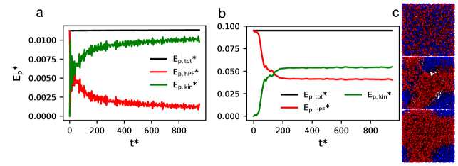
Figure 1: Energy per particle ($E_{\text{p}}^{*}$ as function of time for a system of initially randomly dispersed particles with zero velocity. Panel a: single component system; panel b: binary, phase-separating system; panel c: Representative snapshots along the time evolution of the binary system.

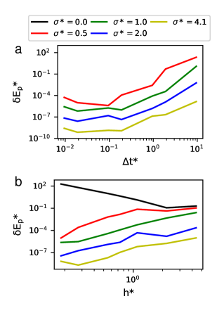
Figure 2: Change in total energy per particle as function of time step $\Delta t^{*}$ (panel a), and grid size $h^{*}$ (panel b), for different values of $\sigma^{*}$.

As an initial test for the ability of the proposed formulation of hPF-MD to conserve energy we consider a system of randomly dispersed particles with initial zero velocity, simulated under $NVE$ conditions. As seen in Figure 1, the system quickly heats up as the potential energy is exchanged with the kinetic energy, while the total energy remains conserved. As expected by using the same interpolation for density and forces,Hockney and Eastwood (1988) the total momentum remains identical to zero throughout the whole simulation (data not shown). The conservation of the energy is perfectly observed also when simulating a binary mixture of repulsive particles, where dramatic structural changes like the progressive phase separation of the two components do not affect the total energy of the system (Figure 1b,c).

The degree of conservation of energy, as with any molecular simulation, will generally depend on the total energy of the molecular system, but here also on the grid size $h^{*}$, time step $\Delta t^{*}$ and $\sigma^{*}$. Figure 2 reports how the conservation of energy depends on these parameters. Using a small grid size $h^{*}$, we can control for the bias due to grid discretization and examine the effect of reducing the time step (Figure 2a). As expected, reducing the time step improves energy conservation. Interestingly, the $\sigma^{*}$ parameter has two important outcomes. First, conservation of energy is improved by increasing $\sigma^{*}$. Second, the plateau, at which decreasing $\Delta t^{*}$ does not improve the energy conservation, is reached for larger time steps. This agrees with the general trend of $\sigma^{*}$ being scale of coarse-graining leading to smoother dynamics, and thereby allowing for larger time steps.

Running simulations using a very small time step and examining the conservation of energy as function of $h^{*}$, we generally observe better convergence by refining the grid (Figure 2b). However, for grids spacing $h^{*}$ larger than 1, corresponding to the specific length between particles, we also obtain a good conservation of energy, even without smoothing. This regime corresponds to standard hPF-MD in which density distribution itself is sufficiently smooth to achieve conservation of the energy. We note if it is desirable to reduce the smoothing obtained by increasing the grid size, one possible solution is to apply an additional sharpeningFeng et al. (2016); Hockney and Eastwood (1988) on the unfiltered densities $\phi$.

III.2 Aliasing

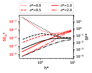
Figure 3: The standard deviation of the energy (red line and axis) and the forces (black lines and axis) averaged over 100 random translations and rotations for a system of $10\,000$ randomly dispersed particles.

To evaluate aliasing due to the grid on the force calculation, we consider the energy and the forces in a reference system of randomly dispersed particles before and after a random rototranslation operation (see Appendix B for more details). We measure the effect of the grid by computing standard deviations of $\delta E^{*}$ and $\delta F^{*}$ (Figure 3). The general trend observed for conservation of the energy as function of $h^{*}$ is also mirrored in Figure 3. Reducing $h^{*}$ reduces aliasing, unless for large $h^{*}>1$, at which the smoothing due to density interpolation itself reduce aliasing. Thus, to avoid significant aliasing, the grid either needs to be smaller than $\sigma^{*}$ or bigger than 1, the average distance between particles.

Figure 4: Time evolution of the sphericity of a droplet of a monoatomic fluid in an imiscible solvent. Snapshots depict the initial organization of the droplet prepared in a cubic shape, and the final spherical organization found by hPF-MD. The solvent phase is not displayed for clarity purposes.

Aliasing in hPF-MD has been particular noticeable when considering molecular aggregates, such as in large vesicles or in droplets, where instead of a spherical shape, a cubic shape oriented according to the grid has been predicted. There are primarily two causes: aliasing due to insufficient grid resolution to represent spherical shapes (such aliases are cured when considering larger systemsVogiatzis, Megariotis, and Theodorou (2017)), and numerical derivatives of the external potential that are not rotational invariantSevink et al. (2017); Nicola et al. (2020). Here, since we can arbitrarily reduce the grid size, and the derivative is estimated in Fourier space, both of these forms of aliasing can be controlled for. To demonstrate this, we here consider the ability of our formulation to predict the sphericity $\Psi$ of a phase-separated droplet:

$$\Psi=\frac{\pi^{1/3}(6V)^{2/3}}{A},$$ (25)

where $V$ and $A$ are the volume and the area of the droplet. Figure 4 reports the time evolution of the sphericity of the droplet from a prepared cubic shape as function of time. As seen, the sphericity quickly increases from $0.90$ to $0.99$, which is close to a perfectly spherical object.

III.3 Quasi-instantaneous approximation

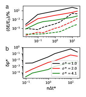
Figure 5: Comparison between quasi-instantaneous approximation (whole lines) integrating $n$ times the equations of motion with time interval $\Delta t^{*}$, and direct integration with a time step $n\Delta t^{*}$ (dashed lines). Panel a: Relative deviation of the total energy. Panel b: Change in average momentum for the quasi-instantaneous approximation. No change in momentum was found using large integration steps.

In SCMF and hPF-MD, the quasi-instantaneous approximation is used to speed up simulations by approximating the external potential as constant between multiple time steps.Daoulas and Müller (2006); Milano and Kawakatsu (2009) For hPF-MD in particular, it can be defined as:

$$\mathbf{F}^{\text{quasi}}_{i}(t,t^{\prime}) =-\int\mbox{\boldmath$\nabla$}V(\mathbf{r},t)P(\mathbf{r}-\mathbf{r}_{i},t^{\prime})\text{d}\mathbf{r},$$ (26)

where $t$ is the time of the external potential update, is $t^{\prime}$ is the time of the force computation ($t\leq t^{\prime}$). A direct measurement of how well the quasi-instantaneous approximation works is obtained by running simulations and recording change in energy and momenta after a certain amount time (Figure 5). The quasi-instantaneous approximation not only produces a net momentum, but also achieves worse conservation of energy than simply using a larger time steps. This is surprising, as it has been demonstrated that such approximation achieves good results in SCMF.Daoulas and Müller (2006) However, contrary to SCMF, hPF-MD approximates forces and not changes in the energy as required by Monte Carlo. While perhaps disappointing, we remark that this approximation is likely to be more relevant for SCMF, which requires a stationary external potential between Monte Carlo moves in order to update multiple particle positions in between external potential updates. The same approximation may not be as much needed in hPF-MD. In this case, when large time steps may be employed, depending on the value of $\sigma^{*}$, a multiple time step algorithm in which particle-field forces are kept constant in between external potential updates and intramolecular potential forces are computed frequently is a promising alternative.Tuckerman, Berne, and Martyna (1992)

III.4 Properties

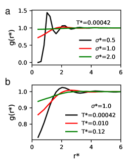
Figure 6: Radial distribution function ($g(r^{*})$) for a single component monoatomic fluid. Panel a: Low temperature behavior for different values of $\sigma^{*}$. Panel b: Temperature dependence of $g(r^{*})$ for $\sigma^{*}=1$.

Particle-field interactions are designed to enforce thermodynamic averages, such as partitioning and local density fluctuations. Nevertheless, the presence of a well defined interaction potential will necessarily introduce some spatial organisation among the molecules composing the system. In Figure 6 we report the radial distribution function for a monoatomic fluid simulated at $NVT$ conditions. We first note that the lower the temperature, the more structure is observed, with the appearance of a solvation shell structure similar to that of a liquid phase. Inspecting the radial distribution function at very low $T^{*}$, which according to our reduced units corresponds to a low level of compressibility, we examine the effect of the smoothing parameter $\sigma^{*}$ on the structure of the fluid. Overall, by lowering $\sigma^{*}$ more structuring is obtained. This effect can be interpreted by considering $\sigma^{*}$ as a measure of the delocalization of the particles. In the limit of $\sigma^{*}\gg 1$, the particles are delocalized in the whole volume; thus, any conformation would produce the same local density equal to the average density, and very little structuring of the fluid. On the contrary, for $\sigma^{*}\sim 0.5$ the particle spread corresponds to the specific length; in this case, an organisation of the particles at a distance $r*~{}1$ will guarantee a homogeneous local density. Instead, any motion will produce fluctuations of the density, and a consequent increase in the energy. As a consequence, the hPF induces strong structuring in the fluid at the characteristic $r^{*}=1$ distance (Figure 6). For lower values of $\sigma^{*}$, particles will be localised more than the range of the external potential, thus the model will produce a behavior similar to that of a diluted gas of small hard spheres. This overall behaviour is consistent with what has been reported for the Gaussian Core modelStillinger and Stillinger (1997); Laradji, Guo, and Zuckermann (1994), indicating a direct correspondence between these two approaches.

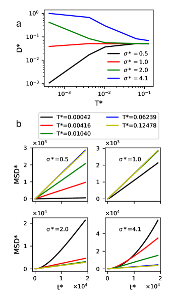
Figure 7: Panel a: Fitted diffusion coefficient ($D^{*}$) for a single component monoatomic fluid as function of $T^{*}$ for different values of $\sigma^{*}$. Panel b corresponding Mean square diplacement (MSD) used to compute the diffusion coefficients.

Using an appropriate Canonical sampling thermostat,Bussi, Donadio, and Parrinello (2007) we investigate the dynamic behavior of the model. In Figure 7 we report both the estimated diffusion coefficient and the mean square deviations for the monophase system at different temperatures. Increasing $\sigma^{*}$ leads to higher diffusion, in line with the results reported by StillingerStillinger and Weber (1978). This is consistent with interactions being smoother, and $\sigma^{*}$ corresponding to a scale of coarse-graining, thereby allowing particles to more easily go unhindered. Despite the simplicity of the model, the diffusion behavior as function of temperature is complex. Contrary to the intuitive increase of diffusion with temperature, which corresponds directly to the thermal velocities of the particles, we here observe here for $\sigma^{*}>1$ a decrease of the diffusion coefficient and for $\sigma^{*}<1$ an increase. A possible explanation of this behavior is that for large $\sigma^{*}>1$ and low temperatures, the motion of the particles becomes close to ballistic, and as temperature is increased the increased thermal velocity is not compensated by the interaction with density fluctuations that hinder the free diffusion of the particles. For low $\sigma^{*}<1$ particles will not move in a smooth density landscape and thus this effect is not present and we have the expected increase in diffusion coefficient with temperature. We note that anomalous diffusion behavior has been reported for Gaussian Core modelsMausbach and May (2006). From a pragmatic point of view, where diffusion is often the limiting step to achieve good equilibration of the systems under study, increasing the $\sigma^{*}$ parameter may be an excellent way of speeding up the dynamics of the system and the overall sampling, and thus to reach preequilibrated configurations in relatively short time.

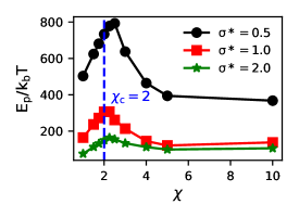
Figure 8: Total energy as a function of $\chi=\tilde{\chi}/k_{\text{b}}T$ for a fluid composed by two repulsive monoatomic species using different $\sigma^{*}$ values. The blue dashed lines reports the theoretical mean field critical value $\chi_{c}$ for the phase separation.

Finally, in Figure 8 we probe how the $\chi$ parameter controls the phase behavior of the binary system by computing the total energy per particle as a function of $\chi$. For all $\sigma^{*}$s, we find a breaking point for the first derivative at around $\chi=2.25$, signaling a phase transition. This value corresponds fairly well to the Flory-Huggins mean field critical point ($\chi=2$). A small overestimation has been previously reported by other hPF approachesPike et al. (2009) and is likely due to finite size effects, as well as our simulations not being mean field. The correct representation of the phase separation thermodynamics for different values of $\sigma^{*}$ is a direct indication that the MD scheme here introduced describes the correct partitioning physics by the hPF model.

IV Conclusions

In this work we have developed a new methodology for achieving Hamiltonian and alias-free hPF-MD. This development is made possible by three main steps. First, the hPF-MD forces is derived by spatial derivative of the interaction energy functional with respect to particle positions. Second, the hPF-MD functional is expressed in terms of filtered densities that converge as the grid is refined. This achieves smooth forces, as well as controlling for aliases. Last, a standard PM FFT-based implementation for the force calculation is used to ensure that the theoretical energy and momentum conservation is achieved.

Through a series of benchmark studies on simple monoatomic species, we demonstrate that the energy and momentum of the particles in the model are both numerically conserved. The conservation of the energy is primarily determined by the appropriate choice for the grid size, time step and spread $\sigma$ used for the filtered densities. In accordance with considering $\sigma$ as a scale of coarse-graining, we find that the larger the spread the larger time steps can be used. If a large enough grid size is used, larger than the typical distance between particles, well behaved forces are also obtained without additional smoothing.

The quasi-instantaneous approximation was examined in detail and benchmarked against using a large time step. We find that this approximation yields worse conservation of the energy, and that it leads to production of nonphysical net momenta. This suggests that while the quasi-instantaneous approximation may work well for Monte Carlo schemes, the same scheme is not ideal for hPF-MD. From an algorithmic point of view, this suggests that a multiple step algorithm with frequent computation of intramolecular forces and infrequent calculation of particle-field forces is a promising alternative. Such an approach would also not require storing the external potential, as it is needed with quasi-instantaneous approximation, and thereby simplifying parallelization and decreasing memory use of current implementations.Zhao et al. (2012)

By studying the properties of model, focusing on the effect of Gaussian spread $\sigma$, we find a good agreement between this implementation of hPF-MD and the literature of Gaussian core models. Generally, we find that increasing the spread of the Gaussian reduces the molecular structure and increases the diffusion of the particles.

In summary, we have presented a new formulation of hPF-MD that guarantees numerical robustness and controlled convergence for energy and force calculations. The natural continuation of this work lies in developing an efficient parallelized implementation that also includes molecular potentials.

V Acknowledgements

Authors acknowledge the support of the Norwegian Research Council through the CoE Hylleraas Centre for Quantum Molecular Sciences (Grant No. 262695) and the Norwegian Supercomputing Program (NOTUR) (Grant No. NN4654K). MC acknowledges funding by the Deutsche Forschungsgemeinschaft (DFG) within the project B5 of the TRR 146 (project number 233630050). Lastly, the authors would like to acknowledge Yu Feng for developing and distributing the PMESH python package, which allowed for a straightforward implementation of the methodology presented in this study.

Data Availability Statement

The data that support the findings of this study are available from the corresponding author upon reasonable request.

Appendix A Equivalence with Gaussian-core model

For simplicity we here consider a single species:

$$W[\tilde{\phi}] =\frac{1}{2\kappa\phi_{0}}\int\tilde{\phi}(\mathbf{r})\tilde{\phi}(\mathbf{r})\text{d}\mathbf{r}$$ (27)

From Plancherel theorem we can rewrite this energy as:

$$W[\tilde{\phi}]=\frac{1}{2\kappa\phi_{0}}\int\hat{\tilde{\phi}}(\mathbf{k})\hat{\tilde{\phi}}(\mathbf{k})\text{d}\mathbf{k}.$$ (28)

Next, inserting for $H$ we find:

$$W[\tilde{\phi}]=\frac{1}{2\kappa\phi_{0}}\int\hat{H}(\mathbf{k})^{2}\hat{\phi}(\mathbf{k})\hat{\phi}(\mathbf{k})\text{d}\mathbf{k}.$$ (29)

Next, considering a general pair interaction:

$$W=\frac{1}{2\kappa\phi_{0}}\int\phi(\mathbf{x})\phi(\mathbf{y})K(\mathbf{x}-\mathbf{y})\text{d}\mathbf{x}\text{d}\mathbf{y},$$ (30)

and rewriting as follows:

$$W=\frac{1}{2\kappa\phi_{0}}\int\left(\int\text{d}\mathbf{x}\phi(\mathbf{x})K(\mathbf{x}-\mathbf{y})\right)\phi(\mathbf{y})\text{d}\mathbf{x},$$ (31)

we again use Plancherel theorem and the convolution theorem for the integral with respect to $\mathbf{x}$:

$$W=\frac{1}{2\kappa\phi_{0}}\int\hat{K}(\mathbf{k})\hat{\phi}(\mathbf{k})\hat{\phi}(\mathbf{k}).$$ (32)

We identify here that:

$$\hat{K}(\mathbf{k})=\hat{H}^{2}(\mathbf{k}).$$ (33)

For a Gaussian core model we have that:

$$K(\mathbf{k})=e^{-\sigma^{2}k^{2}}$$ (34)

Thus the square of the filter corresponds to a Gaussian core model.

Appendix B Simulation setups

This section summarize all the simulation settings used to produce all the figures contained in this manuscript.

Figure 1

Both graphs were obtained with $NVE$ simulations of a initial system of 10000 particles randomly placed inside a box of volume $L^{*}=21.54$. A time step $\Delta t^{*}=0.0019$ and grid spacing $h^{*}=0.36$ was used. Figure 1a has only a single particle type, and employed $\sigma^{*}=1$. Figure 1b,c considered a $$50\text{\,}\mathrm{\char 37\relax}$/$50\text{\,}\mathrm{\char 37\relax}$$ mixture of the two species, and employed $\sigma^{*}=2$ and $\tilde{\chi}^{*}=0.375$.

Figure 2

The system consists of 10648 particles placed centered cubic, in a box of length $L^{*}=23$. Particles are distributed with an velocity distribution corresponding to a Boltzmann distribution with a temperature of $T^{*}=0.125$ and simulations last $t^{*}=94.87$. Figure 2a) employs a $\Delta t^{*}=0.00379$, while Figure 2b) employs a $h^{*}=0.183$.

Figure 3

This figure considers a box extending $2L^{*}$ where a system 10000 particles randomly placed inside cubic cell extending $L^{*}=21.54$. The particles are rotated first by a uniformly distributed rotation and then displaced by a random translation. Rotating back the force, the standard deviation of the forces and the energy is computed over 100 samples. We remark that because of periodic boundary conditions, there is not a rotational invariance, but since we here consider a large box and only have short range interactions, we can do the benchmark as described.

Figure 4

The simulations consider 10000 particles in a box of $L^{*}=21.54$ with a 1500 particles forming as a cube. A $\sigma^{*}=1$ used and $\chi=10$ is used. A time step of $\Delta t^{*}=0.019$, $h^{*}=0.36$ is used. The temperature is controlled by a thermostat with time coupling constant $\tau^{*}=1.9$ at a temperature of $T^{*}=0.010$. The area and the volume of the phase-separated shape, which is used for the sphericity, is calculated using the marching cubes algorithm Lorensen and Cline (1987).

Figure 5

This figure was made considering a system of 10648 particles placed centered cubic in a box of length $L^{*}=23$, with initial velocities corresponding to a Boltzmann distribution of temperature $T^{*}=0.12$. The difference in energy for a $NVE$ simulation is computed after simulations lasting a total time of $t^{*}=19$.

Figure 6 and 7

Both figures consider the same system of 10000 particle of single a type inside a volume $L^{*}=21.54$ for a simulation lasting $t^{*}=18973$ with $h^{*}=0.36$ $\Delta t^{*}=0.095$.

Figure 8

The binary system is composed of 80000 particles (50%/50% mixture) with a box size of $L^{*}=43$, thermostated at $T^{*}=0.124$.. Data is gathered for simulations lasting $t^{*}=18973$ using time step $\Delta t^{*}=0.19$ and grid size $h^{*}=1.09$.

References

References

- Daoulas and Müller (2006) K. C. Daoulas and M. Müller, J. Chem. Phys. 125, 184904 (2006).
- Müller (2011) M. Müller, J. Stat. Phys. 145, 967 (2011).
- Milano and Kawakatsu (2009) G. Milano and T. Kawakatsu, J. Chem. Phys. 130, 214106 (2009).
- Vogiatzis, Megariotis, and Theodorou (2017) G. G. Vogiatzis, G. Megariotis, and D. N. Theodorou, Macromolecules 50, 3004 (2017).
- Zhao et al. (2012) Y. Zhao, A. De Nicola, T. Kawakatsu, and G. Milano, J. Comput. Chem. 33, 868 (2012).
- Schneider and Müller (2019) L. Schneider and M. Müller, Comput. Phys. Commun. 235, 463 (2019).
- Milano, Kawakatsu, and De Nicola (2013) G. Milano, T. Kawakatsu, and A. De Nicola, Phys. Biol. 10, 045007 (2013).
- Soares et al. (2017) T. A. Soares, S. Vanni, G. Milano, and M. Cascella, J. Phys. Chem. Lett. 8, 3586 (2017).
- Cascella and Vanni (2015) M. Cascella and S. Vanni, “Chemical modelling: Applications and theory, vol. 12,” (Royal Society of Chemistry, 2015) pp. 1–52.
- Marrink et al. (2019) S. J. Marrink, V. Corradi, P. C. Souza, H. I. Ingólfsson, D. P. Tieleman, and M. S. Sansom, Chem. Rev. 119, 6184 (2019).
- De Nicola et al. (2016) A. De Nicola, T. Kawakatsu, F. Müller-Plathe, and G. Milano, Eur. Phys. J. Spec. Top. 225, 1817 (2016).
- Zhao et al. (2016) Y. Zhao, M. Byshkin, Y. Cong, T. Kawakatsu, L. Guadagno, A. De Nicola, N. Yu, G. Milano, and B. Dong, Nanoscale 8, 15538 (2016).
- Munaò et al. (2018) G. Munaò, A. Pizzirusso, A. Kalogirou, A. De Nicola, T. Kawakatsu, F. Müller-Plathe, and G. Milano, Nanoscale 10, 21656 (2018).
- Munaò et al. (2019) G. Munaò, A. De Nicola, F. Müller-Plathe, T. Kawakatsu, A. Kalogirou, and G. Milano, Macromolecules 52, 8826 (2019).
- De Nicola et al. (2012) A. De Nicola, Y. Zhao, T. Kawakatsu, D. Roccatano, and G. Milano, Theor. Chem. Acc. 131, 1167 (2012).
- Ledum, Bore, and Cascella (2020) M. Ledum, S. L. Bore, and M. Cascella, Mol. Phys. 0, 1 (2020).
- De Nicola et al. (2011) A. De Nicola, Y. Zhao, T. Kawakatsu, D. Roccatano, and G. Milano, J. Chem. Theory Comput. 7, 2947 (2011).
- Bore, Milano, and Cascella (2018) S. L. Bore, G. Milano, and M. Cascella, J. Chem. Theory Comput. 14, 1120 (2018).
- Zhu et al. (2016) Y.-L. Zhu, Z.-Y. Lu, G. Milano, A.-C. Shi, and Z.-Y. Sun, Phys. Chem. Chem. Phys. 18, 9799 (2016).
- Kolli et al. (2018) H. B. Kolli, A. De Nicola, S. L. Bore, K. Schäfer, G. Diezemann, J. Gauss, T. Kawakatsu, Z.-Y. Lu, Y.-L. Zhu, G. Milano, and M. Cascella, J. Chem. Theory Comput. 14, 4928 (2018).
- Bore et al. (2019) S. L. Bore, H. B. Kolli, T. Kawakatsu, G. Milano, and M. Cascella, J. Chem. Theory Comput. 15, 2033 (2019).
- Nicola et al. (2020) A. D. Nicola, T. A. Soares, D. E. Santos, S. L. Bore, G. A. Sevink, M. Cascella, and G. Milano, Biochim. Biophys. Acta , 129570 (2020).
- Schäfer et al. (2020) K. Schäfer, H. B. Kolli, M. Christensen, S. L. Bore, G. Diezemann, J. Gauss, G. Milano, R. Lund, and M. Cascella, Angew. Chem. (in press, 2020), 10.1002/anie.202004522.
- Carrer et al. (2020) M. Carrer, T. Skrbic, S. L. Bore, G. Milano, M. Cascella, and A. Giacometti, J. Phys. Chem. B (2020), 10.26434/chemrxiv.12388772.v1.
- Bore et al. (2020) S. L. Bore, H. B. Kolli, A. De Nicola, M. Byshkin, T. Kawakatsu, G. Milano, and M. Cascella, J. Chem. Phys 152, 184908 (2020).
- Sevink et al. (2017) G. Sevink, F. Schmid, T. Kawakatsu, and G. Milano, Soft matter 13, 1594 (2017).
- Sgouros et al. (2018) A. Sgouros, A. Lakkas, G. Megariotis, and D. Theodorou, Macromolecules 51, 9798 (2018).
- Pizzirusso et al. (2017) A. Pizzirusso, A. De Nicola, G. A. Sevink, A. Correa, M. Cascella, T. Kawakatsu, M. Rocco, Y. Zhao, M. Celino, and G. Milano, Phys. Chem. Chem. Phys. 19, 29780 (2017).
- Laradji, Guo, and Zuckermann (1994) M. Laradji, H. Guo, and M. J. Zuckermann, Phys. Rev. E 49, 3199 (1994).
- Hockney and Eastwood (1988) R. W. Hockney and J. W. Eastwood, Computer simulation using particles (crc Press, 1988).
- Feng et al. (2016) Y. Feng, M.-Y. Chu, U. Seljak, and P. McDonald, Mon. Not. R. Astron. Soc. 463, 2273 (2016).
- Rapaport and Rapaport (2004) D. C. Rapaport and D. C. R. Rapaport, The art of molecular dynamics simulation (Cambridge university press, 2004).
- Deserno and Holm (1998) M. Deserno and C. Holm, J. Chem. Phys. 109, 7678 (1998).
- Canuto et al. (2006) C. Canuto, M. Y. Hussaini, A. Quarteroni, and T. A. Zang, Spectral methods (Springer, 2006).
- Parzen (1962) E. Parzen, Ann. Math. Stat. 33, 1065 (1962).
- Stillinger and Stillinger (1997) F. H. Stillinger and D. K. Stillinger, Physica A: Statistical Mechanics and its Applications 244, 358 (1997).
- Pike et al. (2009) D. Q. Pike, F. A. Detcheverry, M. Müller, and J. J. de Pablo, J. Chem. Phys. 131, 084903 (2009).
- Swope et al. (1982) W. C. Swope, H. C. Andersen, P. H. Berens, and K. R. Wilson, J. Chem. Phys. 76, 637 (1982).
- Bussi, Donadio, and Parrinello (2007) G. Bussi, D. Donadio, and M. Parrinello, J. Chem. Phys. 126, 014101 (2007).
- Feng, Hand, and biweidai (2017) Y. Feng, N. Hand, and biweidai, “rainwoodman/pmesh 0.1.33,” (2017).
- Tuckerman, Berne, and Martyna (1992) M. Tuckerman, B. J. Berne, and G. J. Martyna, J. Chem. Phys. 97, 1990 (1992).
- Stillinger and Weber (1978) F. H. Stillinger and T. A. Weber, The Journal of Chemical Physics 68, 3837 (1978).
- Mausbach and May (2006) P. Mausbach and H.-O. May, Fluid Ph. Equilibria 249, 17 (2006).
- Lorensen and Cline (1987) W. E. Lorensen and H. E. Cline, ACM siggraph computer graphics 21, 163 (1987).