Towards muon-electron scattering at NNLO
Abstract
The recently proposed MUonE experiment at CERN aims at providing a novel determination of the leading order hadronic contribution to the muon anomalous magnetic moment through the study of elastic muon-electron scattering at relatively small momentum transfer. The anticipated accuracy of the order of 10ppm demands for high-precision predictions, including all the relevant radiative corrections. The theoretical formulation for the fixed-order NNLO photonic radiative corrections is described and the impact of the numerical results obtained with the corresponding Monte Carlo code is discussed for typical event selections of the MUonE experiment. In particular, the gauge-invariant subsets of corrections due to electron radiation as well as to muon radiation are treated exactly. The two-loop contribution due to diagrams where at least two virtual photons connect the electron and muon lines is approximated taking inspiration from the classical Yennie-Frautschi-Suura approach. The calculation and its Monte Carlo implementation pave the way towards the realization of a simulation code incorporating the full set of NNLO corrections matched to multiple photon radiation, that will be ultimately needed for data analysis.
Keywords:
Fixed target experiments, Precision QED, NNLO computations1 Introduction
The value of the anomalous magnetic moment of the muon, , is a fundamental quantity in particle physics, that is presently known with a relative accuracy of 0.54ppm Bennett:2006fi . The muon anomaly, i.e. the deviation of the magnetic moment from the value predicted by Dirac theory, is due to quantum loop corrections stemming from the QED, weak and strong sector of the Standard Model (SM) Jegerlehner:2009ry ; Jegerlehner:2017gek . Hence, the comparison between theory and experiment provides a very stringent test of the SM and a deviation from the SM expectation is a monitor for the detection of possible New Physics signals.
There is a long-standing and puzzling muon discrepancy between the measured value and the theoretical prediction, which presently exceeds the level. The current status of the SM theoretical prediction for the muon has been very recently reviewed in Ref. Aoyama:2020ynm .
Two new experiments, i.e. the presently running E989 experiment at Fermilab Grange:2015fou ; Venanzoni:2014ixa and the E34 experiment under development at J-PARC Iinuma:2011zz ; Mibe:2011zz , are expected to improve the current accuracy by a factor of four. This calls for a major effort on the theory side in order to reduce the uncertainty in the SM prediction, which is dominated by non-perturbative strong interaction effects as given by the leading order hadronic correction, , and the hadronic light-by-light contribution.
Traditionally, has been computed via a dispersion integral of the hadron production cross section in electron-positron annihilation at low energies Jegerlehner:2018zrj ; Keshavarzi:2018mgv ; Davier:2019can . Lattice QCD calculations are providing alternative evaluations of the leading order hadronic contribution DellaMorte:2017dyu ; Borsanyi:2017zdw ; Wittig:2018r ; Meyer:2018til ; Blum:2018mom ; Giusti:2018mdh ; Giusti:2020efo . Very recently the BMW collaboration has presented a precise determination of with an uncertainty of % Borsanyi:2020mff , a central value larger than the ones obtained via dispersive approaches by about and in agreement with the BNL experimental determination Bennett:2006fi . New and promising algorithms are being developed for lattice QCD evaluation of to reduce statistical fluctuations DallaBrida:2020cik . To clarify this situation, alternative and independent methods for the evaluation of are therefore more than welcome.
Following ideas first put forward in Refs. Lautrup:1969uk ; Lautrup:1971jf for the evaluation of as an integral over the photon vacuum-polarization function at negative , a novel approach has been recently proposed to derive from a measurement of the effective electromagnetic coupling constant in the space-like region via scattering data Calame:2015fva . Shortly afterwards, the elastic scattering of high-energy muons on atomic electrons has been identified as an ideal process for such a measurement Abbiendi:2016xup 111A method to measure the running of the QED coupling in the space-like region using small-angle Bhabha scattering was proposed in Ref. Arbuzov:2004wp and applied to LEP data by the OPAL Collaboration Abbiendi:2005rx . and a new experiment, MUonE, has been proposed at CERN to measure the differential cross section of scattering as a function of the space-like squared momentum transfer MUonE:LoI . In order for this new determination of to be competitive with the traditional dispersive approach, the uncertainty in the measurement of the differential cross section must be of the order of 10ppm. This experimental target requires high-precision predictions for scattering, including all the relevant radiative corrections.
The extreme accuracy of MUonE demands for theoretical progress in the calculation of QED corrections to muon-electron scattering, resulting in next-generation Monte Carlo (MC) tools. For ultimate data analysis, the latter will have to include the full set of NNLO QED corrections combined with the leading (and, eventually, next-to-leading) logarithmic contributions due to multiple photon radiation. Quite recently, a number of steps have been already taken to achieve this goal. In Ref. Alacevich:2018vez , the full set of NLO QED and one-loop weak corrections was computed without any approximation and implemented in a fully exclusive MC generator. It is presently being used for simulation studies of MUonE events in the presence of QED radiation. Important results were also obtained at NNLO accuracy in QED. The master integrals for the two-loop planar and non-planar four-point Feynman diagrams were computed in Refs. DiVita:2018nnh ; Mastrolia:2017pfy , by setting the electron mass to zero while retaining full dependence on the muon mass. A general procedure to extract leading electron mass terms for processes with large masses, such as muon-electron scattering, from the corresponding massless amplitude was given in Ref. Engel:2018fsb and supplemented with a subtraction scheme for QED calculations with massive fermions at NNLO accuracy Engel:2019nfw . The two-loop hadronic corrections to scattering were computed in Refs. Fael:2019nsf ; Fael:2018dmz . Also possible contamination from New Physics effects has been studied in Refs. Masiero:2020vxk ; Dev:2020drf . A comprehensive review of the current theoretical knowledge of the muon-electron scattering cross section for MUonE kinematical conditions has been published in Ref. Banerjee:2020tdt .
In this paper, we present the calculation of the fixed-order NNLO QED photonic corrections and its implementation in a fully fledged MC generator (Mesmer, Muon Electron Scattering with Multiple Electromagnetic Radiation 222The MC code is not public yet, but we plan to make it available on a public repository soon.), which represents the first step towards the inclusion of the full set of NNLO corrections matched to multiple photon emission. In Section 2 the gauge invariant subset of photonic corrections on the single fermionic line (electron and muon) are discussed. These contributions are exact at NNLO accuracy, including all mass terms. The extension of the calculation to include the virtual amplitudes involving the interference between the electron and muon line is discussed in Section 3. In this case the two-loop diagrams where at least two virtual photons connect the electron and muon lines are not completely known yet. However, thanks to the universality structure of the infrared (IR) contributions, the IR part of these NNLO virtual contributions can be taken into account by means of the classical Yennie-Frautschi-Suura (YFS) approach Yennie:1961ad . The real radiation matrix elements and phase space are exact, including all fermion mass terms. The described theoretical formulation is included in a fully exclusive NNLO MC code, needed for precision simulations at the MuonE experiment. The structure of the code is completely general and can be easily extended to include the nowadays missing exact NNLO contributions, thus removing the present source of approximation.
We performed several cross checks against the independent calculation of Ref. Banerjee:2020rww for NNLO radiation stemming from the electron leg, finding perfect agreement. Thanks to this common effort, we agreed with the authors of Ref. Banerjee:2020rww to proceed in parallel and make our results public at the same time.
By means of the developed MC code we illustrate in Section 4 numerical results relevant for typical running condition and event selections of the MUonE experiment. In particular, in Section 4.1 we show the impact of the exact NNLO photonic corrections due to electron and muon radiation on the main observables of interest for the MUonE experiment. In Section 4.2 we consider the impact of the approximate full NNLO photonic corrections on a subset of the same observables. In order to roughly estimate the uncertainty of the YFS approximation to the full NNLO amplitudes, a comparison of YFS at NLO is performed against the exact NLO calculation of Ref. Alacevich:2018vez . A summary and future prospects are given in Section 5. The work presented in this paper represents the first fundamental step towards the implementation of a fully-fledged MC generator including the complete set of NNLO corrections matched to multiple photon emission.
2 Electron (and muon) line radiation
The complete set of NNLO QED corrections along the electron line entering the process consists of three parts with contributions due to virtual and real photons. The virtual corrections give rise to ultraviolet divergencies that are computed in Dimensional Regularization (DR) and renormalized using the on-shell renormalization scheme.
The three parts contributing to a given differential cross section at NNLO are the following ones:

All the above contributions are infrared-divergent quantities and we choose to regularize IR singularities by assigning a vanishingly small mass to the photon in the computation of virtual and real contributions. Then we introduce a soft-hard slicing separator , so that it acts as a fictitious energy resolution parameter of the photon radiation phase space, which is split into three sectors: the region labelled as corresponds to the region of unresolved radiation up to , the domain labelled as corresponds to the region with one resolved photon (with energy ) and additional unresolved radiation up to , the domain corresponds to the region with two resolved photons, where both of them have energy larger than . According to the above described splitting, the pure contribution to the cross section can be rewritten as follows:
| (1) |
where
| (2) | ||||
| (3) | ||||
| (4) |
and the subscripts and superscripts of Eqs. (2)-(4) indicate explicitly the number of virtual , soft and hard photons. In Eq. (1), the cross section stands for the one-loop correction to the single bremsstrahlung with emission of a photon of energy greater than . Analogously, is the cross section corresponding to the radiation of two hard photons. The dependence on the photon mass parameter has been made explicit in Eqs. (2) and (3). Each term entering Eq. (1) is independent of . The radiation of real soft photons with energy smaller than is included by means of analytical eikonal factors tHooft:1978jhc ; Denner:1991kt ; Denner:2019vbn . The sum of the right-hand side of Eq. (1) is also independent of , so that Eq. (1) can be used to take into account any realistic experimental event selection.
The master formula with up to NNLO accuracy implemented in our MC generator reads as follows
| (5) |
where and represent the tree-level and the NLO contributions, respectively. For definiteness and later use, we also define
| (6) | ||||
| (7) |
For the calculation of the radiative corrections with one virtual photon and the double bremsstrahlung process, all the Feynman diagrams were manipulated with the help of the algebraic manipulation program Form Kuipers:2012rf ; Ruijl:2017dtg , keeping full dependence on the lepton masses. The evaluation of one-loop tensor coefficients and scalar functions is performed using the package Collier Denner:2016kdg 333Several cross-checks have been performed with the package LoopTools Hahn:2010zi ; Hahn:1998yk finding very good agreement.. As a cross-check, we compared our QED calculation of the one-loop Dirac and Pauli form factors with the Abelian limit of the QCD results given in Ref. Bernreuther:2004ih (see also Gluza:2009yy ), converting the soft-IR pole in DR to the logarithm involving the photon mass according to the rule Denner:2019vbn , finding perfect agreement. For the virtual two-loop corrections, we resorted to the calculation of the QED form factors of Ref. Mastrolia:2003yz , where IR divergences are parameterized in terms of the fictitious photon mass and all finite lepton mass effects are kept 444We thank P. Mastrolia and A. Primo for providing us with updated exact expressions of the form factors.. In the latter, the result is expressed in terms of Harmonic Polylogarithms and we checked that the asymptotic expansion for large momentum transfer agrees with the high-energy limit of the two-loop form factors given in Refs. Berends:1987ab ; Burgers:1985qg , up to constant terms. It is worth mentioning that the QCD NNLO form factors have been calculated also in Ref. Ablinger:2017hst , with partial results relevant for the full three-loop form factor calculation in Refs. Blumlein:2019oas ; Ablinger:2018zwz ; Blumlein:2018tmz ; Ablinger:2018yae .
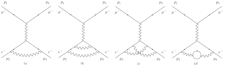
The QED form factors also contain the contribution of the diagram with a vacuum polarization insertion on the vertex photonic correction (see Figure 1, diagram 1d), due to the same lepton of the external legs. This contribution is enhanced by a term proportional to , where represents the collinear logarithm, which is, in any case, exactly cancelled by the emission of a real leptonic pair, when the latter is integrated on the available phase space Montagna:1998vb . For this reason we define our NNLO photonic corrections by removing the contribution due to the fermionic loop, which will be investigated in the future with real leptonic pair emission. This contribution to the Dirac and Pauli form factors has been computed independently in DR and found to agree with Eqs. (94) and (95) of Ref. Bonciani:2004gi . The final result is finite and independent of the regularization scheme adopted in the intermediate steps.
3 YFS-inspired approximation of the full two-loop amplitude
In this section, we discuss how the full two-loop virtual QED corrections can be approximated to catch its complete IR structure. The aim is to implement a full, although approximate, two-loop QED correction to the process which includes correctly at least all the IR parts. In particular, we are approximating only the diagrams obtained by inserting a virtual photon into a QED one-loop box diagram, all the rest of the corrections being exact. We remark that also the full one-loop corrections to the radiative processes are needed and calculated exactly, including box and pentagon diagrams. The latter are calculated with the techniques described above for one-loop corrections 555For the full one-loop QED corrections to the process of single-photon emission, we find agreement with the matrix elements calculated by using the Recola-Collier package Actis:2016mpe ; Denner:2016kdg . Particular attention is being paid in order to make the pentagon amplitudes numerically stable in phase-space regions where the external photon momentum tends to be soft. The details are beyond the scope of the present paper and will be possibly discussed elsewhere..
The full two-loop virtual amplitude is built-up exploiting the YFS analysis of IR divergencies in QED Yennie:1961ad . The starting point are Eqs. (2.2a-c) of the original YFS paper, where the exact -loop amplitude is formally written extracting order by order IR factors in an iterative way. Stopping at two-loop, their equations can be written as
| (8) |
where represents the tree level amplitude, are the exact -loop amplitudes, (of order ) is the YFS IR virtual factor and the superscript R indicates the non-IR remnant of the amplitude. We stress that IR divergencies are confined only in the terms containing at least one factor.
Restricting to the process under consideration and using momenta labelling as in Fig. 1, the IR factor explicitly reads (see also Refs. Jadach:2000ir ; Schonherr:2008av ; Krauss:2018djz ; Linten:2018dpx )
| (9) |
where
| (10) |
| (11) |
In Eq. (10), is the charge of particle in positron charge units, for an incoming (outgoing) fermion and the arguments of the scalar one-loop functions and follow Collier/LoopTools conventions. We stress that with are the factors which factorize the IR divergence of the diagrams obtained by dressing the underlying amplitude with an extra virtual photon attached to the electron () or muon () line or connecting them (). An analogous separation holds for the exact one-loop amplitude and its non-IR remnant of Eq. (8), i.e. we can write .
We can now approximate the complete two-loop virtual amplitude by writing
| (12) |
where in the second line of Eq. (12) we have put . With little algebra, the previous definition can be also recast in the following form
| (13) |
In Eq. (12), in the first row, () represents the set of two-loop diagrams where the two virtual photons are both attached to the electron (muon) line, whereas represents the diagrams where one photon is on the electron line and the other one on the muon line 666This set can be easily computed exactly, for instance by using one-loop renormalized vertex form factors.. The second row contains the full IR part of Eq. (8). The third and fourth rows finally subtract from the second one the IR content already accounted for in . In other words, the approximation misses only the non-IR remnant of the two-loop diagrams where at least two photons connect the electron and muon lines, which are not known yet for the process under consideration. This is made possibly more explicit in the equivalent form of Eq. (13), where each term in the second row, approximately accounting for the missing contributions, has a factor with an “” subscript. Despite being incomplete, the exact IR structure of the full two-loop amplitude, with massive electron and muon, is present in Eqs. (12) and (13): on the one side this can be used to cross-check the IR part of the final calculation once it is available, on the other side it can be implemented into the Monte Carlo generator for phenomenological studies. We stress that, when we add to the rest of the exact contributions, the sum is perfectly independent of the fictitious photon mass and thus the result is meaningful.
On the accuracy side, heuristic considerations, also based upon an analogous numerical analysis at one-loop order, bring us to estimate the size of the dominant missing non-IR corrections to be in the range of a few , as discussed later.
4 Numerical results
In this Section, we show and discuss the phenomenological results obtained by using a fully differential MC code, Mesmer, which implements the theoretical approach described in Section 2 and Section 3. We adopt the parameters and typical running condition of the MUonE experiment already described in detail in Ref. Alacevich:2018vez , which we briefly remind here: the reference frame is the laboratory frame, where the energy of the incoming is GeV, the electron is assumed to be at rest inside a bulk target and thus . In this kinematical condition, the collinear logarithms and are of the order of and , respectively. We study the numerical impact of QED NNLO photonic corrections to observables assuming the following event selections (Setup 2 and Setup 4 of Ref. Alacevich:2018vez ):
-
1.
and GeV (i.e. ). The angular cuts model the typical acceptance conditions of the experiment and the electron energy threshold is imposed to guarantee the presence of two charged tracks in the detector (Setup 1);
-
2.
the same criteria as above, with the additional acoplanarity cut . We remind the reader that this event selection is considered in order to mimic an experimental cut which allows to stay close to the elasticity curve given by the tree-level relation between the electron and muon scattering angles (Setup 2)777The acoplanarity cut partially removes radiative events and thus enhances the fraction of quasi-elastic events, as illustrated by Fig. 3 of Ref. Alacevich:2018vez . Here it is used merely as a possible cut for selecting elastic events, without pretending it to be realistic. Indeed, from the experimental point of view, the extraction of the hadronic contribution to the running of could benefit from selecting events in the elastic region.,
where , and are the scattering and azimuthal angles and the energy, in the laboratory frame, of the outgoing electron and muon, respectively.
For Setup 1 and Setup 3 of Ref. Alacevich:2018vez , with GeV, the NNLO QED photonic effects are similar in size to the ones presented here and therefore are not considered for the sake of brevity.
The input parameters for the simulations are set to
and the considered differential observables are the following ones:
| (14) |
where .
For definiteness, we remark that all calculations and simulations are performed in the center of mass (c.m.) frame and then the momenta are boosted to the laboratory frame, where the initial-state electron is at rest. The soft-hard separator , not Lorentz invariant, is defined in the c.m. reference frame and its default value is taken to be . We checked both at integrated and differential level that the cross-sections are independent of the unphysical parameters and .
Within the full set of NLO and NNLO QED corrections, there are three gauge-invariant subsets of photonic contributions corresponding to:
-
1.
virtual and real corrections along the electron line;
-
2.
virtual and real corrections along the muon line;
-
3.
the rest of the virtual and real corrections, including box-like contributions, up-down interference of real photon radiation and so on.
In Section 4.1 we present the exact QED NNLO photonic corrections for the distributions of Eq. (14) for the electron and muon line separately. In Section 4.2 we present the results for our approximation to the full QED NNLO virtual photonic corrections described in Sect. 3 888We remind the reader that in our approximation any real radiation contribution is exact, including all finite mass effects.. All the figures show the difference in per cent between the NNLO and NLO predictions relative to the tree-level differential cross section, i.e.
| (15) |
where stand for electron-line only, muon-line only and the full set of NNLO corrections. For the sake of clarity, all the figures contain insets which display the NLO corrections w.r.t. the LO predictions, according to
| (16) |
In order to quantify the purely photonic effects, we do not include any vacuum polarization correction neither in the NLO nor in the NNLO cross sections. The absolute values and shapes of the observables can be obtained from Ref. Alacevich:2018vez . In this Section, figures with two panels show corrections in Setup 1 on the left and in Setup 2 on the right, unless stated otherwise.
| (b) | Setup 1 | Setup 2 | ||
|---|---|---|---|---|
| 255.1176(5) | 255.8437(5) | 222.8545(3) | 222.7714(3) | |
Before showing the effects on the distributions, we quote in Tab. 1 the integrated cross-sections for the two Setups, showing the different classes of corrections. The symbols stand for the cross sections with corrections along the electron line only, along the muon line only and the full approximate contributions, respectively, with the perturbative accuracy given by the subscripts. The subsets of corrections coming from electron or muon line separately are the same for both processes and , as expected. For Setup 1 the correction to the cross section along the electron line amounts to less than 0.01% with positive sign, with respect to the NLO prediction, while the correction along the muon line is below the level, still compatible with zero within the statistical integration uncertainty. For Setup 2 the correction along the electron line becomes of the order of % and the one along the muon line below the % level. The numbers in the last row of the table are italicized to indicate that these cross-sections are approximate according to the discussion of Sect. 3. Numerically, the full corrections in Setup 1 amount to about %, with respect to the NLO prediction, for the process with beam, while it amounts to about % with in the initial state. Given the inherent uncertainty, roughly estimated to be of the order of % in Section 3, these estimates can not be considered conclusive yet. When including the acoplanarity cut (Setup 2), the approximate NNLO corrections become of the order of %, because of IR effects enhancement, thus being more robust in view of the intrinsic uncertainty of the approximate prediction discussed before.
4.1 Exact NNLO corrections from one leptonic line
In this Section we present the results for the relative contribution of the NNLO photonic corrections to the differential distributions according to Eq. (15). In particular, we consider the exact NNLO corrections due to electron and muon radiation, which represent different gauge invariant subsets of the whole NNLO corrections. The correction along the electron line is particularly important, because, as shown in Ref. Alacevich:2018vez , already at NLO level it is enhanced w.r.t. the radiation from the muon line, as a consequence of the small ratio . Moreover, it gives the bulk of the correction for some observables or in particular phase-space regions.
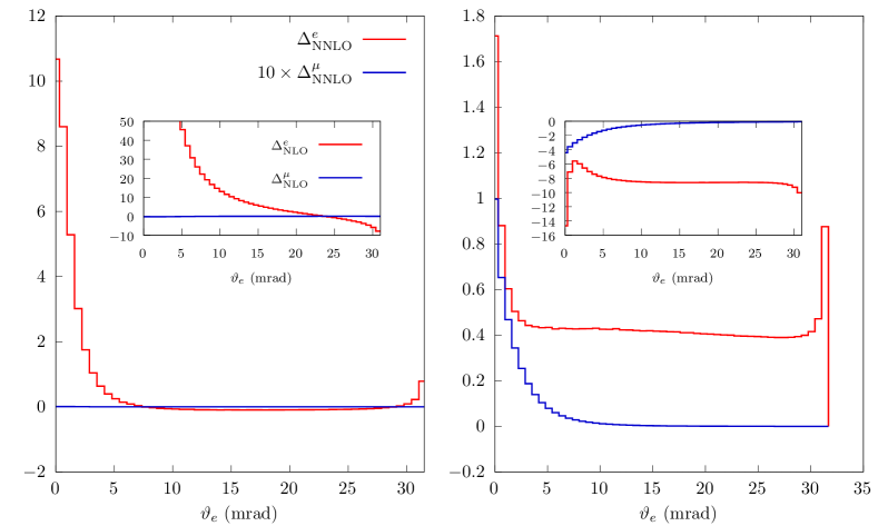
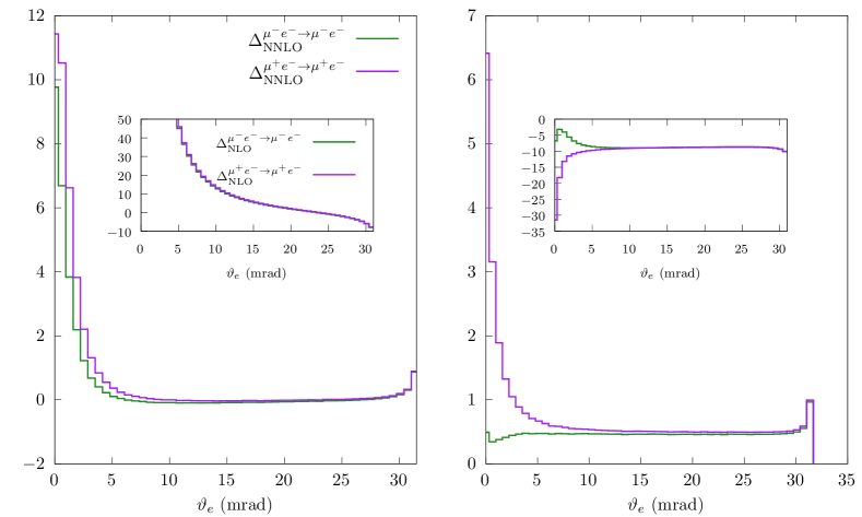
Figure 3 shows the effects of NNLO corrections, according to Eq. (15), for the observable . In Setup 1, the correction along the electron line (red histogram) is flat over a large portion of scattering angles larger than about mrad, being of the order of a few at most, and displays a steep increase for , where it reaches the order of . As can be seen from the inset, the electron scattering angle distribution is quite sensitive to NLO corrections, in particular for small values of , where the NLO correction becomes particularly enhanced as due to hard bremsstrahlung effects and because the tree-level differential cross section tends to zero. As a consequence, the increase of the NNLO correction for is not surprising. Contrarily to the correction along the electron line, the one along the muon line (blue histogram, multiplied by a factor of 10) is flat over the whole angular spectrum and invisible on the plot scale. The shape of the corrections remains qualitatively the same also in the presence of the additional acoplanarity cut of Setup 2, even if the size of the correction along the electron line becomes larger () for a wide range of . This is a consequence of the effects of the IR enhancement introduced effectively by the acoplanarity cut. Indeed the NLO correction grows to negative values of the order of . In Setup 2, the NNLO correction due to electron radiation is about for mrad and amounts to at the opposite kinematical boundary. Even in the presence of the acoplanarity cut, the NNLO correction along the muon line remains flat over the entire spectrum, increasing to about for , consistently with the behaviour of the NLO correction shown in the inset.
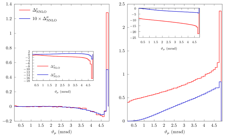
Figure 4 shows the effects of NNLO corrections for the observable 999In this case, we do not show muon scattering angles because the corrections are huge and would spoil the readability of the plots. The reason for this feature is that the LO prediction becomes negligible in the above angular range, as a consequence of the applied acceptance cuts, while the single- and double-radiative events populate the region.. In Setup 1 (left panel), the NNLO correction along the electron line (red histogram) has a non-trivial shape, remaining of the order of and dropping to about from mrad to mrad, with a sharp increase in the last two bins, reaching the level of at the kinematical limit. Interestingly, the NNLO correction along the muon line (blue histogram) displays the same shape of the correction along the electron line but with a reduction in size by a factor of ten (a factor of 30 in the last bin). The shapes of the corrections change when the acoplanarity cut is added (right panel). In this case the correction along the electron line (red histogram) becomes an increasing function of , ranging from for in the left corner of the plot to about at the upper kinematical limit. This large and positive correction can be understood by looking at the inset, which shows that the NLO correction varies monotonically between and , as enhanced by IR effects introduced by the acoplanarity cut. The NNLO correction along the muon line displays qualitatively a similar shape and reaches about at the upper kinematical limit.
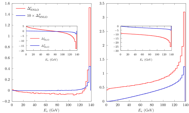
Figure 5 shows the effects of NNLO corrections for the observable . In Setup 1, the NNLO correction along the electron line is negative, not exceeding the level up to energies of the order of GeV, where it shows a change of slope towards positive values, reaching the level of for the maximum available energy. This feature reflects the behaviour of the NLO correction, shown in the inset, which ranges from to in the region GeV and drops to about at the kinematical limit, signalling the presence of enhanced IR effects because of missing available phase space for real photon emission. For Setup 2, the IR enhancement of the NNLO corrections is visible over the entire energy range, changing monotonically from about for to about at the upper kinematical limit. The NNLO correction along the muon line is similar in shape to the one along the electron line but with reduced size by about a factor of .
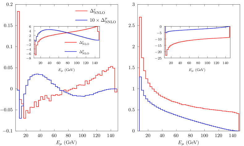
In Fig. 6 we show the effects of NNLO corrections on . In the case of Setup 1, the shapes of the contributions along the electron line (red histogram) and the muon line (blue histogram) are quite different. The former displays a sharp peak, of the order of in the first bin for the minimum muon energy and then ranges monotonically from up to about . The correction along the muon line shows a more rich structure, never exceeding the size of . When including the acoplanarity cut (Setup 2), the NNLO correction along the electron line becomes a monotonically decreasing function of , ranging from to about . The NNLO correction along the muon line (in blue) displays qualitatively a similar behaviour.
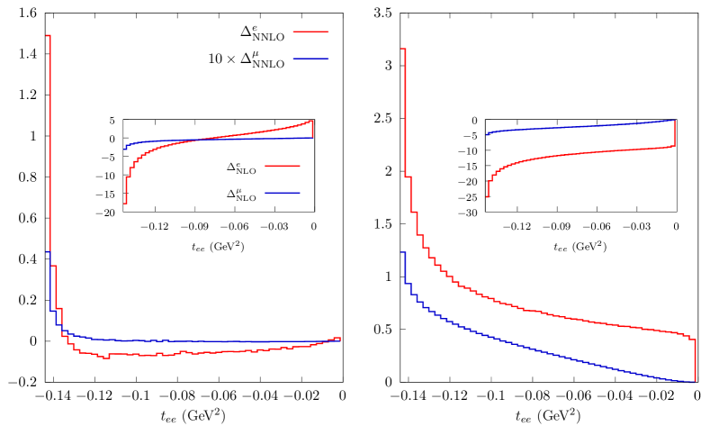
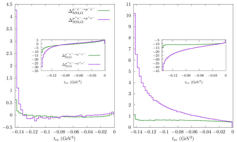
Figure 7 shows the size of NNLO corrections on . In Setup 1, the correction along the electron line (red histogram) is slightly negative, never exceeding the -0.1% level, for GeV2. For comparison, it is worth noticing that the NLO correction changes by about , by looking at red line in the inset. For lower values (larger absolute values) of , the correction shows a steep increase to positive values, reaching about at the kinematical boundary, where the NLO correction reaches about w.r.t. the tree-level prediction. The NNLO correction along the muon line (blue histogram) displays a similar behaviour, as a function of , but with much smaller size: it does not exceed the level in the window GeV2 and reaches the size of about at the kinematical boundary. The right panel of Fig. 7 shows the NNLO corrections when the acoplanarity cut is added (Setup 2). The electron-line correction is positive and increasing with increasing , from about up to at the boundary. This can be expected since the corresponding NLO correction on the electron line ranges from about to , because of the increased importance of the IR logarithm in the presence of cuts that tend to suppress hard photon emission. Also the NNLO correction along the muon line (blue histogram) is enhanced in the right panel ranging from about up to . Correspondingly, the NLO correction shown in the inset ranges from to .
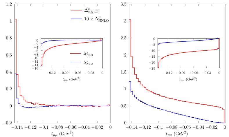
Finally, in Fig. 8 we consider the size of NNLO corrections on . The behaviour of the corrections, as functions of , is similar to those of Fig. 7. In particular, for Setup 1, the correction along the electron (muon) line ranges from about % to at the kinematical boundary. Also in the presence of the acoplanarity cut of Setup 2 (right panel), the shapes of the corrections are similar to the ones of Fig. 7, ranging from about to along the electron (muon) line.
4.2 Approximation to the full NNLO corrections
In Fig. 9, to be compared to Fig. 3, we show how the full (approximate) NNLO correction impacts the distribution. In absence of the acoplanarity cut (Setup 1, left panel), we notice how the NNLO correction is similar to the one stemming only from the electron line, except that at the left corner of the distribution is a few larger for the initiated process and smaller of a similar amount when is in the initial state. A more dramatic change is visible in Setup 2, when the acoplanarity cut is applied. For the case, the NNLO corrections are similar to the electron-line corrections above , but grow to as . For the case instead, also in the region the NNLO correction remains moderate at the level and almost flat. We remark that an analogous difference between and is present also at NLO (see the insets and Figs. 10 and 11 of Ref. Alacevich:2018vez ) and that NNLO corrections tend to reduce the NLO ones. The variation in the corrections for different charge of the muon can be ascribed to different radiation patterns, which interfere destructively in one case and constructively in the other one.
We finally show the NNLO effects on the distribution in Fig. 10, to be compared to Fig. 7. Also in this case, for Setup 1, the largest differences w.r.t. the corrections coming only from electron line occur for close to the kinematical limit , where the phase space allowed for radiation is restricted and IR effects are enhanced. For Setup 2, NNLO corrections are almost flat and of order for incoming , while increase in size going from order to as goes from to for incoming .
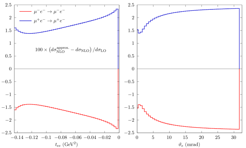
After discussing the numerical impact of the approximate full two-loop amplitude of Sect. 3 on relevant distributions, we conclude by examining its theoretical accuracy, which is necessarily an educated estimate since the exact calculation is not available yet. Firstly, we show how the one-loop box diagrams are approximated by their IR part as obtained from the YFS approach. In other terms, we compare the exact NLO virtual amplitude of Eq. (8) with the approximation
| (17) |
which can be thought as the NLO version of Eq. (13), or, otherwise, the latter can be seen as the NNLO generalization of the former. In Fig. 11, the difference of the exact NLO differential cross section and the approximate one, relative to LO, is shown as a function of the (left) and (right) variables. We remark that the difference depends on the charge of the incoming muon, as expected, but does not depend on the acoplanarity cut because only the virtual amplitude is modified. The approximation differs from the exact result at the level of -. We notice that this is of the same order of . This simple observation brings us to estimate the accuracy of Eq. (13) for the full two-loop amplitude to be of the order of .
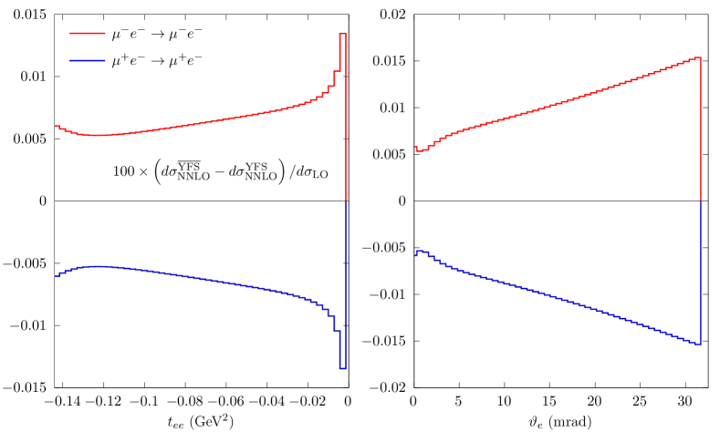
Our estimate is further corroborated by noticing that the IR separation implied by Eq. (8) is not unique because non IR-terms can be freely moved from the factors to the remnants. In our case, where we necessarily set for diagrams with at least two photons connecting the and lines, we can for instance switch off some non-IR terms in the second line of Eq. (13) to probe the size of the missing non-IR terms. For the sake of illustration, we accomplish this by setting to zero non-IR terms (which are also not singular in the limit of vanishing lepton masses) in the functions appearing in Eq. (10). More explicitly, in the expression of the IR function (see Eq. (B.5) of Ref. Dittmaier:2003bc )
| (18) |
where , is the vanishing photon mass and is defined in Eq. (B.7) of Ref. Dittmaier:2003bc , we remove the finite terms in second and third line of Eq. (18). We label this further NNLO approximation as and in Fig. 12 we compare it to the standard one at differential level on the and distributions. The plots show that the (IR-safe) differences lie below the range (in LO units), of the same size of the above estimate based on the NLO result.
5 Summary and prospects
In this work, we have analyzed the NNLO photonic corrections to scattering and presented phenomenological results obtained with a related MC code, named Mesmer. The study is motivated by the recent proposal of measuring the effective electromagnetic coupling constant in the space-like region by using this process (MUonE experiment). From the measurement of the hadronic contribution to the running of , the leading hadronic contribution to the muon anomaly can be derived according to an alternative approach to the standard time-like evaluation of .
The calculation features the exact NNLO contribution of the gauge-invariant subset of QED photonic corrections along the leptonic legs, including all finite mass terms. The IR divergences are regularized by means of a small photon mass and a slicing photon energy parameter to separate soft from hard real radiation. The contribution of the vertex vacuum polarization insertion has been removed, in order to avoid potentially large logarithmic contributions which are cancelled by the real radiation of leptonic pairs, leaving the issue to a future investigation. The complete NNLO calculation, i.e. including also the up-down radiation contribution, has been calculated in an approximate way, since the complete NNLO virtual amplitudes are not yet available in the literature. Nevertheless, a YFS approach allows to approximate the missing NNLO virtual amplitudes with the correct inclusion of all IR enhanced terms. Moreover, the double-real radiation matrix elements as well as the phase space are exact, including all finite lepton mass effects. Also the NLO corrections to the process, which are a part of the NNLO calculation, are exact.
The developed formalism has been implemented in a fixed-order generator able to reach NNLO accuracy for any differential cross sections. The structure of the code is completely general and the YFS approximation to the two-loop diagrams with at least two virtual photons connecting the electron and muon lines can easily be replaced with the corresponding exact amplitude, once available.
By means of the developed MC generator, we have extended a recent analysis from the NLO to the NNLO accuracy. In particular, we have considered a threshold electron energy of 1 GeV in the laboratory frame and two basic reference event selections: one involving only typical acceptance cuts of the MUonE experimental detector for the final state electron and muon; one including also a simplified acoplanarity cut to restrict the events around the elasticity curve given by the tree-level correlation between final state electron and muon scattering angles. We have considered a number of differential distributions, which allow to fully characterize the events of the MUonE experiment and to outline the best data analysis strategy to extract the HLO contribution to the running of the electromagnetic coupling constant in the space-like region.
The phenomenological study of the different observables points out that the size of the NNLO corrections, w.r.t. the LO differential cross-sections, is at the level of a few for several regions of phase space in the presence of acceptance cuts only, leaving some corners of phase space where the corrections can grow up to the per cent level. As already remarked in the previous NLO analysis, the only exception is the electron scattering angle distribution which is particularly sensitive to photon radiation, in the region of small scattering angles where the LO prediction tends to zero as . A similar feature of the LO prediction is also present for the muon scattering angle distribution, but in a very small range around . Moreover, the typical size of the NNLO corrections grows up to the order of a few per mille in the presence of the acoplanarity cut, reaching the several per cent level at the boundaries of the phase space. This is a signal that IR terms start to dominate over the rest of the matrix elements (as already noticed in the NLO analysis) and definitely points to the relevance of the next step of matching the fixed order calculation with an all order exclusive resummation procedure of multi-photon emission, for instance by generalizing to NNLO accuracy the matching of NLO corrections with a QED Parton Shower of Ref. Balossini:2006wc . This step is left to future work and it is by now under consideration.
Acknowledgements.
We are sincerely grateful to all our MUonE colleagues for stimulating collaboration and many useful discussions, which are the framework of the present study. In particular we thank the PSI/Zurich group (P. Banerjee, T. Engel, A. Signer and Y. Ulrich) for continuous exchange and careful cross-check of our results, which helped to validate the technical precision of the developed Monte Carlo program. We are also indebted to P. Mastrolia and A. Primo for providing us with updated expressions of the two-loop form factors. The work of M.C. has been supported by the “Investissements d’avenir, Labex ENIGMASS”.References
- (1) Muon g-2 Collaboration, G. W. Bennett et al., Final Report of the Muon E821 Anomalous Magnetic Moment Measurement at BNL, Phys. Rev. D73 (2006) 072003, [hep-ex/0602035].
- (2) F. Jegerlehner and A. Nyffeler, The Muon g-2, Phys. Rept. 477 (2009) 1–110, [0902.3360].
- (3) F. Jegerlehner, The Anomalous Magnetic Moment of the Muon, Springer Tracts Mod. Phys. 274 (2017) pp. 1–693.
- (4) T. Aoyama et al., The anomalous magnetic moment of the muon in the Standard Model, 2006.04822.
- (5) Muon g-2 Collaboration, J. Grange et al., Muon (g-2) Technical Design Report, 1501.06858.
- (6) Fermilab E989 Collaboration, G. Venanzoni, The New Muon g-2 experiment at Fermilab, Nucl. Part. Phys. Proc. 273-275 (2016) 584–588, [1411.2555].
- (7) J-PARC muon g-2/EDM Collaboration, H. Iinuma, New approach to the muon g-2 and EDM experiment at J-PARC, J. Phys. Conf. Ser. 295 (2011) 012032.
- (8) J-PARC g-2 Collaboration, T. Mibe, Measurement of muon g-2 and EDM with an ultra-cold muon beam at J-PARC, Nucl. Phys. Proc. Suppl. 218 (2011) 242–246.
- (9) F. Jegerlehner, The Muon g-2 in Progress, Acta Phys. Polon. B49 (2018) 1157, [1804.07409].
- (10) A. Keshavarzi, D. Nomura, and T. Teubner, The muon and : a new data-based analysis, Phys. Rev. D97 (2018), no. 11 114025, [1802.02995].
- (11) M. Davier, A. Hoecker, B. Malaescu, and Z. Zhang, A new evaluation of the hadronic vacuum polarisation contributions to the muon anomalous magnetic moment and to , Eur. Phys. J. C 80 (2020), no. 3 241, [1908.00921]. [Erratum: Eur.Phys.J.C 80, 410 (2020)].
- (12) M. Della Morte, A. Francis, V. Gülpers, G. Herdoiza, G. von Hippel, H. Horch, B. Jäger, H. B. Meyer, A. Nyffeler, and H. Wittig, The hadronic vacuum polarization contribution to the muon from lattice QCD, JHEP 10 (2017) 020, [1705.01775].
- (13) Budapest-Marseille-Wuppertal Collaboration, S. Borsanyi et al., Hadronic vacuum polarization contribution to the anomalous magnetic moments of leptons from first principles, Phys. Rev. Lett. 121 (2018), no. 2 022002, [1711.04980].
- (14) H. B. Meyer and H. Wittig, Lattice QCD and the anomalous magnetic moment of the muon, 1807.09370.
- (15) H. B. Meyer and H. Wittig, Lattice QCD and the anomalous magnetic moment of the muon, Prog. Part. Nucl. Phys. 104 (2019) 46–96, [1807.09370].
- (16) RBC, UKQCD Collaboration, T. Blum, P. A. Boyle, V. Gülpers, T. Izubuchi, L. Jin, C. Jung, A. Jüttner, C. Lehner, A. Portelli, and J. T. Tsang, Calculation of the hadronic vacuum polarization contribution to the muon anomalous magnetic moment, Phys. Rev. Lett. 121 (2018), no. 2 022003, [1801.07224].
- (17) D. Giusti, F. Sanfilippo, and S. Simula, Light-quark contribution to the leading hadronic vacuum polarization term of the muon from twisted-mass fermions, Phys. Rev. D 98 (2018), no. 11 114504, [1808.00887].
- (18) D. Giusti and S. Simula, Ratios of the hadronic contributions to the lepton from Lattice QCD+QED simulations, 2003.12086.
- (19) S. Borsanyi et al., Leading-order hadronic vacuum polarization contribution to the muon magnetic momentfrom lattice QCD, 2002.12347.
- (20) M. Dalla Brida, L. Giusti, T. Harris, and M. Pepe, Multi-level Monte Carlo computation of the hadronic vacuum polarization contribution to , 2007.02973.
- (21) B. Lautrup and E. de Rafael, On sixth-order radiative corrections to the muon -Factor, Nuovo Cim. A 64 (1969) 322–324.
- (22) B. Lautrup, A. Peterman, and E. de Rafael, Recent developments in the comparison between theory and experiments in quantum electrodynamics, Phys. Rept. 3 (1972) 193–260.
- (23) C. M. Carloni Calame, M. Passera, L. Trentadue, and G. Venanzoni, A new approach to evaluate the leading hadronic corrections to the muon -2, Phys. Lett. B746 (2015) 325–329, [1504.02228].
- (24) G. Abbiendi et al., Measuring the leading hadronic contribution to the muon g-2 via scattering, Eur. Phys. J. C77 (2017), no. 3 139, [1609.08987].
- (25) A. B. Arbuzov, D. Haidt, C. Matteuzzi, M. Paganoni, and L. Trentadue, The Running of the electromagnetic coupling alpha in small angle Bhabha scattering, Eur. Phys. J. C34 (2004) 267–275, [hep-ph/0402211].
- (26) OPAL Collaboration, G. Abbiendi et al., Measurement of the running of the QED coupling in small-angle Bhabha scattering at LEP, Eur. Phys. J. C45 (2006) 1–21, [hep-ex/0505072].
- (27) MUonE Collaboration, G. Abbiendi et al., Letter of Intent: the MUonE project, Tech. Rep. CERN-SPSC-2019-026, SPSC-I-252, CERN, Geneva, Jun, 2019.
- (28) M. Alacevich, C. M. Carloni Calame, M. Chiesa, G. Montagna, O. Nicrosini, and F. Piccinini, Muon-electron scattering at NLO, JHEP 02 (2019) 155, [1811.06743].
- (29) S. Di Vita, S. Laporta, P. Mastrolia, A. Primo, and U. Schubert, Master integrals for the NNLO virtual corrections to scattering in QED: the non-planar graphs, 1806.08241.
- (30) P. Mastrolia, M. Passera, A. Primo, and U. Schubert, Master integrals for the NNLO virtual corrections to scattering in QED: the planar graphs, JHEP 11 (2017) 198, [1709.07435].
- (31) T. Engel, C. Gnendiger, A. Signer, and Y. Ulrich, Small-mass effects in heavy-to-light form factors, JHEP 02 (2019) 118, [1811.06461].
- (32) T. Engel, A. Signer, and Y. Ulrich, A subtraction scheme for massive QED, JHEP 01 (2020) 085, [1909.10244].
- (33) M. Fael and M. Passera, Muon-Electron Scattering at Next-To-Next-To-Leading Order: The Hadronic Corrections, Phys. Rev. Lett. 122 (2019), no. 19 192001, [1901.03106].
- (34) M. Fael, Hadronic corrections to - scattering at NNLO with space-like data, JHEP 02 (2019) 027, [1808.08233].
- (35) A. Masiero, P. Paradisi, and M. Passera, New physics at the MUonE experiment at CERN, 2002.05418.
- (36) P. B. Dev, W. Rodejohann, X.-J. Xu, and Y. Zhang, MUonE sensitivity to new physics explanations of the muon anomalous magnetic moment, JHEP 05 (2020) 053, [2002.04822].
- (37) P. Banerjee et al., Theory for muon-electron scattering @ 10ppm: A report of the MUonE theory initiative, Eur. Phys. J. C 80 (2020), no. 6 591, [2004.13663].
- (38) D. R. Yennie, S. C. Frautschi, and H. Suura, The infrared divergence phenomena and high-energy processes, Annals Phys. 13 (1961) 379–452.
- (39) P. Banerjee, T. Engel, A. Signer, and Y. Ulrich, QED at NNLO with McMule, SciPost Phys. 9 (2020) 027, [2007.01654].
- (40) G. ’t Hooft and M. J. G. Veltman, Scalar One Loop Integrals, Nucl. Phys. B153 (1979) 365–401.
- (41) A. Denner, Techniques for calculation of electroweak radiative corrections at the one loop level and results for W physics at LEP-200, Fortsch. Phys. 41 (1993) 307–420, [0709.1075].
- (42) A. Denner and S. Dittmaier, Electroweak Radiative Corrections for Collider Physics, Phys. Rept. 864 (2020) 1–163, [1912.06823].
- (43) J. Kuipers, T. Ueda, J. A. M. Vermaseren, and J. Vollinga, FORM version 4.0, Comput. Phys. Commun. 184 (2013) 1453–1467, [1203.6543].
- (44) B. Ruijl, T. Ueda, and J. Vermaseren, FORM version 4.2, 1707.06453.
- (45) A. Denner, S. Dittmaier, and L. Hofer, Collier: a fortran-based Complex One-Loop LIbrary in Extended Regularizations, Comput. Phys. Commun. 212 (2017) 220–238, [1604.06792].
- (46) T. Hahn, Feynman Diagram Calculations with FeynArts, FormCalc, and LoopTools, PoS ACAT2010 (2010) 078, [1006.2231].
- (47) T. Hahn and M. Perez-Victoria, Automatized one loop calculations in four-dimensions and D-dimensions, Comput. Phys. Commun. 118 (1999) 153–165, [hep-ph/9807565].
- (48) W. Bernreuther, R. Bonciani, T. Gehrmann, R. Heinesch, T. Leineweber, P. Mastrolia, and E. Remiddi, Two-loop QCD corrections to the heavy quark form-factors: The Vector contributions, Nucl. Phys. B706 (2005) 245–324, [hep-ph/0406046].
- (49) J. Gluza, A. Mitov, S. Moch, and T. Riemann, The QCD form factor of heavy quarks at NNLO, JHEP 07 (2009) 001, [0905.1137].
- (50) P. Mastrolia and E. Remiddi, Two loop form-factors in QED, Nucl. Phys. B664 (2003) 341–356, [hep-ph/0302162].
- (51) F. A. Berends, W. L. van Neerven, and G. J. H. Burgers, Higher Order Radiative Corrections at LEP Energies, Nucl. Phys. B297 (1988) 429. [Erratum: Nucl. Phys.B304,921(1988)].
- (52) G. J. H. Burgers, On the Two Loop QED Vertex Correction in the High-energy Limit, Phys. Lett. 164B (1985) 167–169.
- (53) J. Ablinger, A. Behring, J. Blümlein, G. Falcioni, A. De Freitas, P. Marquard, N. Rana, and C. Schneider, Heavy quark form factors at two loops, Phys. Rev. D 97 (2018), no. 9 094022, [1712.09889].
- (54) J. Blümlein, P. Marquard, N. Rana, and C. Schneider, The Heavy Fermion Contributions to the Massive Three Loop Form Factors, Nucl. Phys. B 949 (2019) 114751, [1908.00357].
- (55) J. Ablinger, J. Blümlein, P. Marquard, N. Rana, and C. Schneider, Automated Solution of First Order Factorizable Systems of Differential Equations in One Variable, Nucl. Phys. B 939 (2019) 253–291, [1810.12261].
- (56) J. Blümlein, P. Marquard, and N. Rana, Asymptotic behavior of the heavy quark form factors at higher order, Phys. Rev. D 99 (2019), no. 1 016013, [1810.08943].
- (57) J. Ablinger, J. Blümlein, P. Marquard, N. Rana, and C. Schneider, Heavy Quark Form Factors at Three Loops in the Planar Limit, Phys. Lett. B 782 (2018) 528–532, [1804.07313].
- (58) G. Montagna, M. Moretti, O. Nicrosini, A. Pallavicini, and F. Piccinini, Light pair correction to Bhabha scattering at small angle, Nucl. Phys. B547 (1999) 39–59, [hep-ph/9811436].
- (59) R. Bonciani, A. Ferroglia, P. Mastrolia, E. Remiddi, and J. J. van der Bij, Two-loop N(F)=1 QED Bhabha scattering differential cross section, Nucl. Phys. B701 (2004) 121–179, [hep-ph/0405275].
- (60) S. Actis, A. Denner, L. Hofer, J.-N. Lang, A. Scharf, and S. Uccirati, RECOLA: REcursive Computation of One-Loop Amplitudes, Comput. Phys. Commun. 214 (2017) 140–173, [1605.01090].
- (61) S. Jadach, B. Ward, and Z. Was, Coherent exclusive exponentiation for precision Monte Carlo calculations, Phys. Rev. D 63 (2001) 113009, [hep-ph/0006359].
- (62) M. Schönherr and F. Krauss, Soft Photon Radiation in Particle Decays in SHERPA, JHEP 12 (2008) 018, [0810.5071].
- (63) F. Krauss, J. M. Lindert, R. Linten, and M. Schönherr, Accurate simulation of W, Z and Higgs boson decays in Sherpa, Eur. Phys. J. C 79 (2019), no. 2 143, [1809.10650].
- (64) R. Linten, Precision simulations in Drell-Yan production processes. PhD thesis, Durham U. (main), 2018.
- (65) S. Dittmaier, Separation of soft and collinear singularities from one loop N point integrals, Nucl. Phys. B 675 (2003) 447–466, [hep-ph/0308246].
- (66) G. Balossini, C. M. Carloni Calame, G. Montagna, O. Nicrosini, and F. Piccinini, Matching perturbative and parton shower corrections to Bhabha process at flavour factories, Nucl. Phys. B758 (2006) 227–253, [hep-ph/0607181].