The Global Landscape of Neural Networks: An Overview

Abstract

One of the major concerns for neural network training is that the non-convexity of the associated loss functions may cause bad landscape. The recent success of neural networks suggests that their loss landscape is not too bad, but what specific results do we know about the landscape? In this article, we review recent findings and results on the global landscape of neural networks. First, we point out that wide neural nets may have sub-optimal local minima under certain assumptions. Second, we discuss a few rigorous results on the geometric properties of wide networks such as “no bad basin”, and some modifications that eliminate sub-optimal local minima and/or decreasing paths to infinity. Third, we discuss visualization and empirical explorations of the landscape for practical neural nets. Finally, we briefly discuss some convergence results and their relation to landscape results.

I Introduction

Deep neural networks have led to remarkable empirical successes in various artificial intelligence tasks, sparking an interest in the theory behind their architectures and training. In the early days when the power of neural networks were not fully harnessed, researchers favored models such as supporting vector machines which could be studied using convex optimization techniques. A major concern in the case of neural networks is that the non-convexity of the associated loss functions may cause complicated and strange optimization landscapes. However, recent experience shows that neural networks can often be trained to find the global minima of appropriately chosen loss functions, thus it is of great interest to understand the loss landscape of neural networks.

A closely related problem is to understand the landscape of the objectives in non-convex matrix problems. In this context, it has been established that the landscape is benign (e.g., every local minimum is a global minimum) for quite a few matrix problems, such as matrix completion and phase retrieval, under certain assumptions (see, e.g., [10] for a survey). Although there are still many cases that remain difficult to analyze, there is much optimism that non-convex matrix problems (under proper assumptions) often have benign landscapes.

For the landscape of neural networks, the status is less clear. One might be interested in getting a “yes” or “no” answer to questions such as “does a neural network have sub-optimal local minima?”, or “can a neural-net problem be solved to find global minima?”. Much progress has been made, but a fully satisfying answer is still not available. We hope this article can explain the existing results in a coherent way so that they are relatively easy to understand.

Compared to another recent survey [46], this article focuses on global landscape and contains formal theorem statements, while [46] covered many aspects of neural net optimization and did not present formal theorems. We suggest readers unfamiliar with neural-net optimization to read [46] for a big picture, and read this article for more in-depth understanding of the global landscape. We focus on results that can apply to deep nets, thus we do not discuss many results on shallow nets which are reviewed in [46] (there is a restriction on the number of references from the journal, so we only select a subset of references in this article).

I-A Summary

The goal of this survey is to provide an overview of the recent progress on the global landscape of neural networks. The central questions to answer are:

• Q1: How to explain the good performance of neural-net optimization algorithms, despite the non-convexity?

• Q2 (rigorous evidence for Q1): To prove a rigorous result, what conditions are needed, and what property can be established?

• Q3: How to design the system so that a rigorous theory can be established?

Based on these high-level questions, we organize the existing results in a flow as follows.

• An initial explanation is Hypothesis 1: “every local-min is a global-min”. The first rigorous evidence is that deep linear networks have no sub-optimal local minima, under mild conditions (Sec. III).

• However, practitioners find that narrow neural-nets cannot be solved well, while over-parameterized neural-nets can. Thus researchers believe that a crucial condition is “over-parameterization”. Results on linear networks do not utilize this condition, thus are not enough to explain practice.

• For non-linear over-parameterized neural nets, sub-optimal local-min can exist under certain assumptions (Sec. IV-C). An alternative Hypothesis 2 is that local descent algorithms “avoid” sub-optimal local-min in neural-net training.

• One explanation of Hypothesis 2 is the following. For many over-parameterized neural-nets no “bad valleys/basins” exist (Sec. IV-D). Thus even if sub-optimal local minima exist, they cannot be strong attractors and thus iterates will not be attracted to them (see Sec. VII-A for such a conjecture).

• With stronger assumptions (e.g. ultra-wide nets), it can be rigorously proved that gradient descent can avoid reaching the area with sub-optimal local minima, thus converging to global minima (Sec. VII-C). Due to space reason, we only touch the surface of this sub-area in this article.

• The above research assumes no modification of the neural-net landscape. If we are allowed to design the landscape (e.g., adding regularizers), then proving “every local-min is global-min” becomes possible for a wide range of neural networks (Sec. VI-B). We further discuss a result that ensures the absence of both bad local-min and decreasing path to infinity (Sec. VI-C).

• Finally, what is the lesson for empirical training? Successful training of neural-nets requires proper initialization, batch normalization, residual connection and wide/deep networks (see [46] for a more thorough survey). The current article focuses on one empirical lesson: large width is important for successful training. For practitioners, many theoretical results in this article can be viewed as evidence of this lesson.

I-B Big picture: the role of landscape analysis

Landscape analysis has been a subject of study since 1980’s; see [8] for an overview. The concern that gradient descent can get stuck at bad local minima has been around for a long time. For instance, Minsky and Papert commented in Perceptrons (expanded edition) that “they speak as though becoming trapped on local maxima were rarely a serious problem” and “we conjecture … will become increasingly intractable as we increase the numbers of input variables”. Reference [8] argued that to address Minky and Papert’s comment, it is “very interesting to investigate the presence of local minima”. Our survey can be viewed as a modern version of the survey [8], by including new results and new understanding, especially results on deep networks. In particular, we will point out that a main claim reviewed in [8] that “over-parameterized 1-hidden-layer network have no sub-optimal local minima” is not rigorous.

The theory of machine learning (for supervised learning) consists of three parts: representation, optimization and generalization. One way to interpret this partition is via the lens of error decomposition: the test error can be decomposed as the sum of representation error, optimization error and generalization error. Landscape analysis is an important component of understanding the optimization error. The optimization error refers to $F(\hat{w})-F^{*}$, where $F$ is the loss function, $\hat{w}$ is the solution (i.e, the parameters of the neural network) found by an algorithm, and $F^{*}$ is the the globally minimal loss. Define $w^{\infty}$ to be a converged solution if the algorithm runs for infinite time and assume it converges. The optimization error can be further decomposed into two parts:

$$[F(\hat{w})-F(w^{\infty})]+[F(w^{\infty})-F^{*}].$$

The first part is the “non-convergence error”, which occurs because either the algorithm is intrinsically not convergent or the algorithm has not converged yet due to limited running time. It is often reasonable to assume $w^{\infty}$ is a stationary point or even a local-min. The second part is the “infinite-time error”, which indicates how far away the converged value is from the global minima value. If every local-min is a global-min, and $w^{\infty}$ is a local minimum, then this term becomes $0$. Proving the convergence of an algorithm is a central task of classical optimization, but it often does not cover the “infinite-time error”. Therefore, landscape analysis provides an understanding of the fundamental limit of the loss function, and is somewhat similar to Shannon’s capacity bound : it indicates how well an algorithm can possibly perform with long training time.

Although our focus is on landscape analysis, we will briefly discuss how a good landscape can possibly lead to the convergence to global-min. Another important topic is the relation of optimization and generalization, such as implicit regularization (e.g. [41, 35]) and the conjecture that wide minima generalize better (e.g. [27]). Due to space, we do not discuss generalization in this article.

II Models

In this section, we present the optimization formulation for a supervised learning problem. Consider input instances $x_{i}\in\mathbb{R}^{d_{x}}$ and output instances $y_{i}\in\mathbb{R}^{d_{y}},i=1,\dots,n$, where $n$ is the number of samples. The goal is to build a model that can predict $y_{i}$ based on $x_{i}$. We use a neural network $f_{\theta}:\mathbb{R}^{d_{x}}\rightarrow\mathbb{R}^{d_{y}}$ to produce a prediction $\hat{y}$ based on an input $x$. For most parts of the article, we consider a fully-connected neural network

$$f_{\theta}(x)=W_{L}\phi(W_{L-1}\dots{\\ }\phi(W_{2}\phi(W_{1}x+b_{1})+b_{2})\dots+b_{L-1}),$$ (1)

where $\phi:\mathbb{R}\rightarrow\mathbb{R}$ is the neuron activation function (or simply “activation”), $W_{j}$ is a matrix of dimension $d_{j}\times d_{j-1}$, $j=1,\dots,L$ and $\theta=(W_{1},b_{1},\dots,W_{L-1},b_{L-1},W_{L})$ is the collection of all parameters. Note that we denote $d_{0}=d_{x}$ and $d_{L}=d_{y}$. We will use $\phi(Z)$ to denote a matrix with each entry $\phi(Z)_{ij}$ being $\phi(Z_{ij}).$

For a certain loss $\ell(\cdot,\cdot)$, the problem of finding the optimal parameters can be written as

$$\min_{\theta}F(\theta)\triangleq\frac{1}{n}\sum_{i=1}^{n}\ell(y_{i},f_{\theta}(x_{i})).$$ (2)

For regression problems, $\ell(y,z)$ is often the quadratic loss $\ell(y,z)=\|y-z\|^{2}$. For binary classification problem, a popular choice of $\ell$ is the logistic loss $\ell(y,z)=\log(1+\exp(-yz))$.

Finally, we present a few standard definitions. We say $\bar{\theta}$ is a global minimum (or simply global-min) of function $F$ iff $F(\bar{\theta})\leq F(\theta),\forall\;\theta.$ We say $\bar{\theta}$ is a critical point of function $F$ iff $\nabla F(\bar{\theta})=0.$ We say $\hat{\theta}$ is a local minimum (or simply local-min) of a function $F(\theta)$ iff there exists an open set $B$ that contains $\hat{\theta}$ such that $F(\hat{\theta})\leq F(\theta),\forall\theta\in B$. We say $\hat{\theta}$ is a strict local-min if the inequality is strict for any other $\theta\in B$. The local maximum can be defined in a similar way (replacing $\leq$ by $\geq$). We say $\hat{\theta}$ is a saddle point iff it is a critical point and neither a local minimum nor a local maximum.

III Linear neural networks

The initial hypothesis is that “every local-min is global-min” in practical neural-nets. The results on linear neural networks were considered early evidence (though not strong), thus historically important. Besides the historical reasons, studying linear networks can help develop technical tools. We remark that linear neural networks are rarely used in practice since their representation power is the same as a linear model, so non-theory readers can skip this section if not interested.

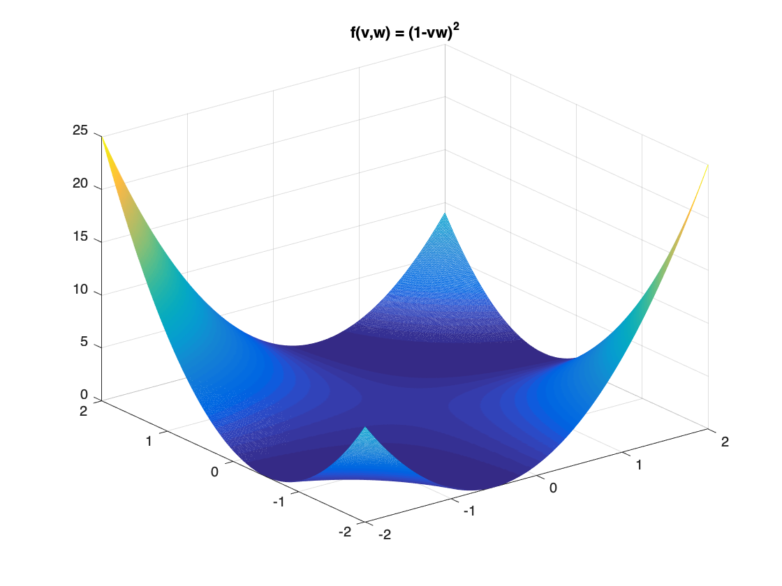
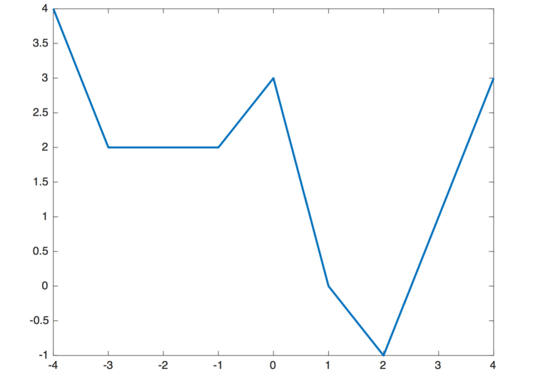
Toy example. We consider the simplest linear neural network problem

$$\min_{v,w\in\mathbb{R}}(vw-1)^{2}.$$

This is a non-convex problem, but it is easy to prove that every local minimum is a global minimum. We plot the function and its contour in Figure 1.

Figure 1: The loss surface of $f(v,w)=(1-vw)^{2}$. All global minima lie in the two curved regions in dark blue.

Hamiltonian of a spin-glass system. Choromanska et al. [12] analyzed the global landscape of multi-layer networks. The motivation was to study a multi-layer network with ReLU activations, but the ReLU activations are removed by adding a somewhat unrealistic assumption, thus essentially converting the network into a multi-layer linear network. Under a few other assumptions, the loss function is transformed to a polynomial function $\sum_{i_{1},\dots,i_{L}=1}^{p}X_{i_{1},i_{2},\dots,i_{L}}w_{i_{1}}\dots w_{i_{L}}$ with Gaussian random coefficients $X_{i_{1},i_{2},\dots,i_{L}}$.

Definition III.1.

(index) The index of a critical point is the number of negative eigenvalues of the Hessian at this point.

They computed the limit of the expected number of stationary points with a given index as the width $p$ goes to infinity. Based on the calculations, they described a layered structure for stationary points with different indices: low-index stationary points (including local minima) are closer to global minima than high-index stationary points (the precise statement is highly technical and omitted here). While their neural network model is somewhat far from practice, the description of the landscape is rather unique and not seen in other works .

Deep linear networks. Kawaguchi [25] extended an early work [7] on 2-layer linear networks to deep linear networks, showing that every local minimum is a global minimum. More specifically, the following problem was studied:

$$\text{P}_{1}:\quad\min_{W_{1},W_{2},\dots,W_{L}}\|Y-W_{L}W_{L-1}\dots W_{1}X\|_{F}^{2},$$ (3)

where $W_{i}\in\mathbb{R}^{d_{i}\times d_{i-1}},i=1,\dots,L$. [25, Theorem 2.3] is the first landscape result on this problem; below we state a slightly stronger version in [39].

Theorem III.1.

[39] Suppose $X$ and $Y$ have full row rank, then every local minimum of the problem (3) is a global minimum.

The proof of [25] is rather complicated, and [39] provided a simpler and more intuitive proof. The idea of [39] is to view the optimization problem (3) as a re-parameterization of a “mother” problem $\text{P}_{2}:$ $\min_{\text{rank}(R)\leq p}\|Y-RX\|_{F}^{2}$ where $p=\min\{d_{0},d_{1},\dots,d_{L}\}$. Note that the effective search space of the original problem $\{W_{L}\dots W_{2}W_{1}\mid W_{i}\in\mathbb{R}^{d_{i}\times d_{i-1}}\}$ is the same as the new search space $\{R:\text{rank}(R)\leq p\}$, which is why we call P2 a “mother problem”. The first step is to prove that any local-min of $P_{1}$ achieves the value of a local-min of $\text{P}_{2}$, and the second step is to prove that $\text{P}_{2}$ has no sub-optimal local-min.

Characterization of all critical points. [49] and [51] provided a more precise characterization of the critical points of deep linear networks. We briefly discuss the results of [49] for the problem (3).

Theorem III.2.

[49] Assume $d_{x}\leq n,d_{y}\leq n$, $XX^{T}$ and $XY^{T}$ are full rank, $YX^{T}(XX^{T})^{-1}X$ has distinct singular values. Further, assume the thinnest layer is the input or the output layer, i.e.,

$$\min_{0\leq i\leq L}d_{i}=\min\{d_{x},d_{y}\}.$$ (4)

For the problem (3), every critical point $(W_{L},\dots,W_{1})$ with the product $W_{L}\dots W_{2}W_{1}$ being full rank is a global minimum, and every critical point with $W_{L}\dots W_{2}W_{1}$ being singular is a saddle point.

The result listed above has a rather clean conclusion: it links full-rankness to global minima. Full-rankness will appear in the analysis of non-linear networks too, which we discuss later.

IV Over-parameterized Networks

A major goal of theoretical research is to identify critical factors of modern neural networks that contribute to successful training. Nowadays, it is commonly believed that large width is one such factor. One evidence is the empirical observation that wide networks are easier to train than narrow networks (e.g. achieving smaller training and test error). Another evidence is that pruned models can achieve similar performance to the original model (e.g., [21]), implying that there are many redundant parameters to help optimization. It is thus an interesting theoretical question whether over-parameterization indeed leads to a benign landscape.

In this section, we discuss the landscape of deep over-parameterized networks (more precisely, wide networks).

IV-A Toy example: single neuron

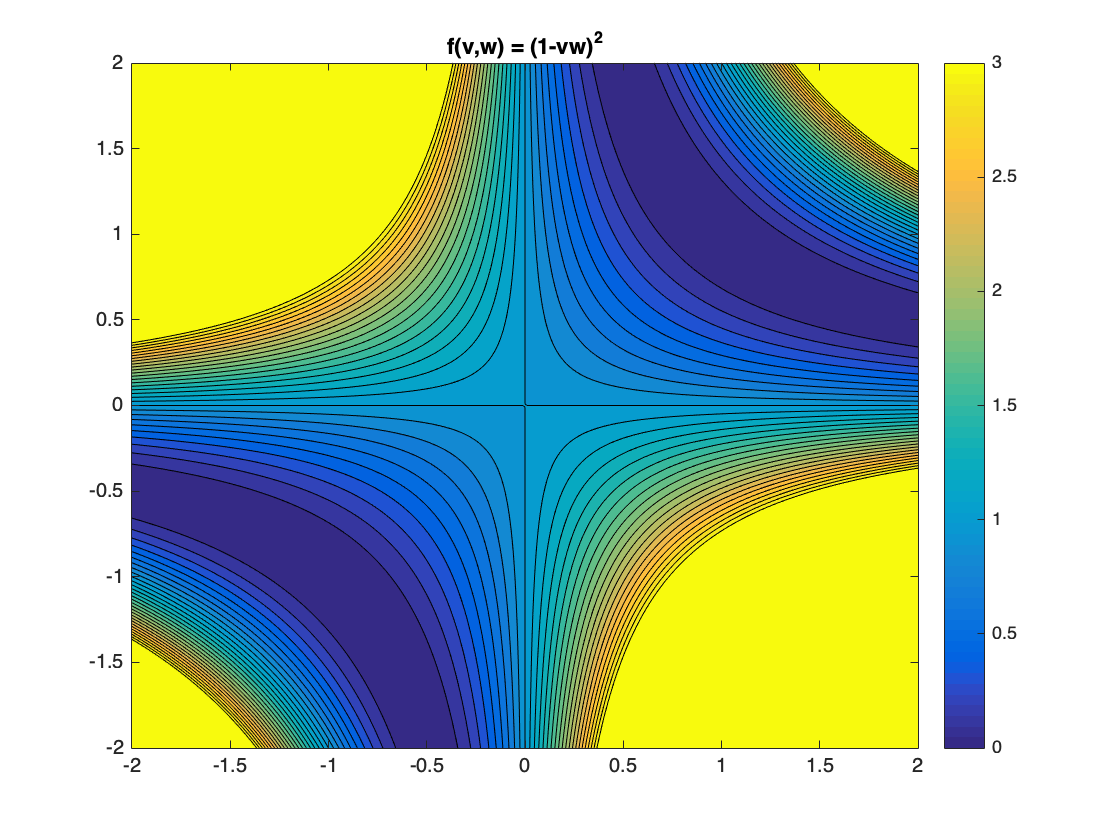
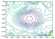
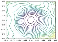
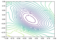
As a toy example, we consider the case $n=d_{1}=1$, i.e., a single sample and a non-linear network with a single neuron. Suppose the associated objective function is $\min_{v,w\in\mathbb{R}}(1-v\phi(w))^{2}.$ We visualize the landscape for a special activation in Figure 2, and it shows that there are infinitely many sub-optimal local minima.

The following result describes the landscape of the above toy model for general activation functions.

Figure 2: The loss surface of $\min_{v,w\in\mathbb{R}}(y-v\phi(wx))^{2}$ with $(x,y)=(1,1)$, and $\phi(z)=-(z-1)^{2}/8$. The red point $(v,W)=(1,1)$ is a sub-optimal local minimum, but it is not a strict local-min (flat along one direction, and curved along the orthogonal direction).

Proposition IV.1.

[14] Suppose $x,y\in\mathbb{R}\backslash\{0\}$. The function $F(w,v)=(y-v\phi(wx))^{2}$ where $v,w\in\mathbb{R}$ has no sub-optimal local minima if and only if the following condition holds: if $\phi(t)=0$, then $t$ is not a local minimum or local maximum of $\phi$.

This result shows that the landscape depends on the neuron activation. For instance, if $\phi(t)=\max\{t,0\}$ (ReLU activation) or $\phi(t)=t^{2}$, then sub-optimal local-min exists; if $\phi(t)=t^{2}+1$ or $\phi$ is strictly increasing, then there is no sub-optimal local-min. When $x$ and $y$ are in high-dimensional space, what conditions guarantee the non-existence of sub-optimal local minima are still not fully understood, though partial progress has been made. In the next two subsections, we discuss a few results for more general neural-nets.

IV-B Bad local-min for ReLU networks

Due to the popularity of ReLU activation, a few works analyzed 2-layer ReLU networks. For instance, [37] [45] constructed sub-optimal local minima for 2-layer ReLU networks under different settings. The existence of sub-optimal local minima for ReLU networks is not surprising, since Proposition IV.1 showed that even for single-neuron network with ReLU activation, sub-optimal local-min can exist. Nevertheless, a rigorous analysis for multi-neuron ReLU networks is non-trivial and requires other techniques. Due to space reason, we do not review these results in detail here.

IV-C Does over-parameterization eliminate bad local-min, for smooth neurons?

One major result reviewed in the survey [8] is that a wide one-hidden-layer network has no sub-optimal local minima. At that time, researchers thought the assumption of “many hidden neurons” is restricted. Nowadays, this assumption is considered rather reasonable, thus it is worthwhile to revisit this classical result more carefully. [8] did not cite the full result, and we cite the version of [48] below.

Claim IV.1.

[48, Theorem 3] Consider the problem $\min_{v\in\mathbb{R}^{1\times p},W\in\mathbb{R}^{p\times d_{x}}}\sum_{i=1}^{n}(y_{i}-v\phi(Wx_{i}))^{2}$, where $\phi$ is a sigmoid function. Assume the width $p\geq n$, and there is one index $k$ such that $x_{ik}\neq x_{jk}$, $\forall i\not=j$. Then every local minimum is a global minimum.

Unfortunately, it was recently found that the claim did not hold. A counter-example to this claim was given in [14]. A modification to this claim will be discussed later.

Cavity of the proof of Claim IV.1. To prove Claim IV.1, [48] first proved the function satisfies the following property (called “Property PT” for short).

Definition IV.1.

(Property PT) We say a function $F$ satisfies Property PT if starting from any point $\theta$, there exists an arbitrarily small perturbation such that from the perturbed point $\hat{\theta}$, there exists a strictly decreasing path to a global minimum.

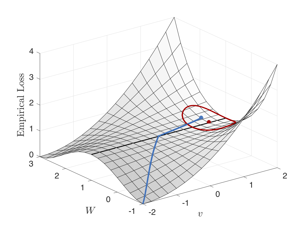
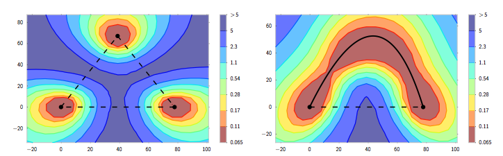
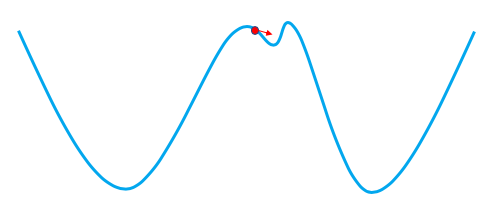
[48] claimed that Property PT implies the non-existence of sub-optimal local minimum. This deduction contains a cavity, as demonstrated in Figure 2. If starting from a sub-optimal local-min (red point), after a small perturbation (the blue point), there is a strictly decreasing path (colored in blue) to the global minimum. Therefore, even if the function satisfies Property PT, sub-optimal local minimum can still exist.

Existence of sub-optimal local-min for arbitrarily wide networks.

The cavity of the proof of ClaimIV.1 does not imply the claim itself does not hold, since there may be other proof methods. Nevertheless, [14] proved that Claim IV.1 does not hold by providing a counter-example.

Proposition IV.2.

Let $n\geq 3$. For a neural network with sigmoid activation and input data $x_{1},\cdots,x_{n}\in\mathbb{R}$ where $x_{i}\neq x_{j}$ for all $i\neq j$, there exists output data $y_{1},\cdots,y_{n}$ such that the empirical loss has a sub-optimal local minimum.

Besides the sigmoid activation, [14] also proved a stronger negative result that for a large class of smooth activation functions, arbitrarily wide and deep networks, generic input data $x_{i}$’s with dimension $d_{x}^{2}+3d_{x}/2<n$, there exist output data $y_{i}$’s such that sub-optimal local minima exist. It is unknown whether allowing picking labels (e.g. label smoothing) can eliminate sub-optimal local-min.

IV-D Absence of bad valleys and basins

Although sub-optimal local-min can exist for wide neural networks, researchers indeed found that a large width is critical for good performance. Thus one may expect that wide networks exhibit some nice geometrical properties. In this subsection, we review results on such properties.

No spurious valley for increasing activations.

Definition IV.2.

A spurious valley is a connected component of a sub-level set $\{\theta:F(\theta)\leq c\}$ which does not contain a global minimum of the loss $F(\theta)$.

The non-existence of spurious valley guarantees the non-existence of sub-optimal strict local-min. Although there may still exist sub-optimal non-strict local minima, the absence of spurious valley ensures that starting from any of these sub-optimal local-min, there exists a non-decreasing path (not necessarily strictly decreasing path) to a region with smaller loss [47].

Reference [47] proved that no spurious valley exists (implying no bad basin) for 1-hidden-layer network with “low intrinsic dimension”. Reference [42] further proved that there is no spurious valley for wide deep neural networks where the last hidden layer has no less neurons than the number of samples, under a few assumptions on the activation functions. This is given in the following theorem.

Theorem IV.1.

Suppose that an arbitrarily deep fully connected neural network $f_{\theta}(x)$ satisfies the following assumptions:

• The activation function $\sigma$ is strictly monotonic and $\sigma(\mathbb{R})=\mathbb{R}$;

• For any integer $p\geq 2$, there do not exist non-zero coefficients $(\lambda_{i},a_{i})^{p}_{i=1}$ with $a_{i}\not=a_{j}$, $\forall i\not=j$, such that $\sigma(x)=\sum^{p}_{i=1}\lambda_{i}\sigma(x-a_{i})$ for every $x\in\mathbb{R}$;

• $d_{L-1}\geq n$;

• All the training samples are distinct.

Then the empirical loss $F(\theta)$ has no spurious valleys.

No sub-optimal basin for any continuous activations. The “no spurious valley” result in [44] holds for strictly increasing analytic activation functions, but it does not cover many non-smooth or non-monotone activations that are commonly applied in practice, such as leaky ReLU or swish. Reference [32] analyzed deep over-parameterized neural networks with any continuous activations. The result relies on a notion called setwise strict local minimum, defined below.

Definition IV.3 (Setwise strict local minimum).

We say a compact subset $X\in S$ is a strict local minimum of $f:S\rightarrow\mathbb{R}$ in the sense of sets if there exists $\varepsilon>0$ such that for all $x\in X$ and for all $y\in S\setminus X$ satisfying $\|x-y\|_{2}\leq\varepsilon$, it holds that $f(x)<f(y)$.

Figure 3: An example of a function without sub-optimal basin (left) and a function with sub-optimal basin (right). Both functions have bad non-strict local minima, consisting a plateau of $(-3,-1)$. Notice that the plateau in the right figure lies in a sub-optimal basin. Source: reprinted from [32].

Definition IV.3 generalizes the notion of strict local minimum from the sense of points to the sense of sets. Subsequently, we introduce the concept of sub-optimal basin.

Definition IV.4.

A sub-optimal basin of a function $f:S\rightarrow\mathbb{R}$ is a setwise strict local minimum that does not contain a global minimum of $f$.

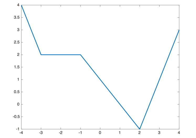
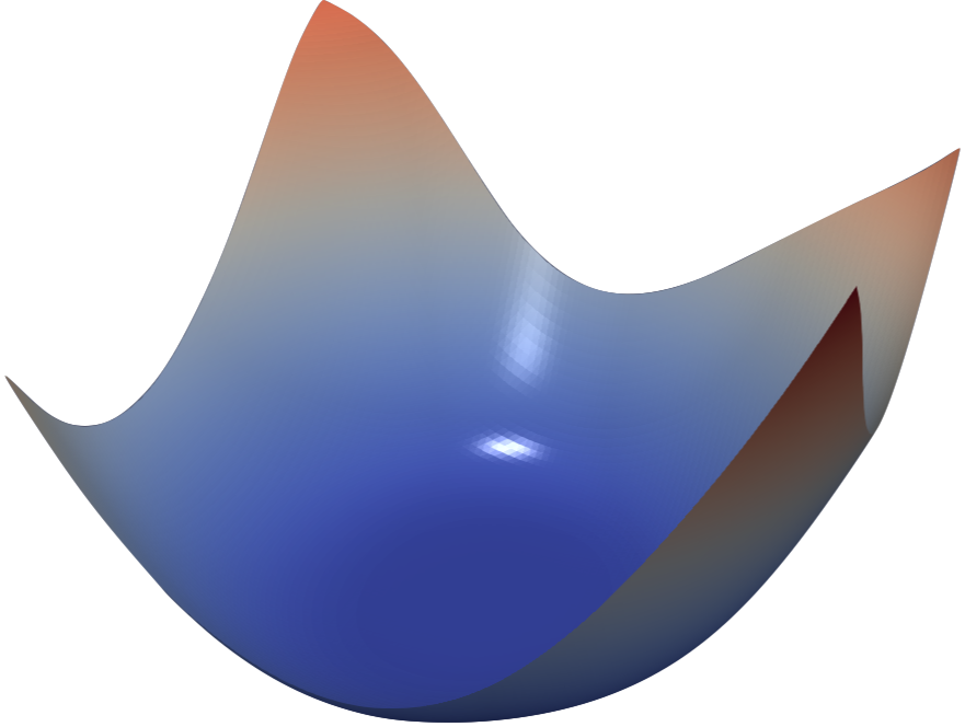
A function that has no sub-optimal basin may still have (pointwise) sup-optimal local minima, which can only form flat areas called “plateaus”. We note that such plateau cannot lie in a bottom of a sub-optimal basin, as illustrated in Figure 3. Reference [32] proved that for all deep neural networks where the last hidden layer is wider than the number of samples, the loss function has no sub-optimal basin.

Theorem IV.2.

Suppose that an arbitrarily deep fully connected neural network $f_{\theta}(x)$ satisfies the following assumptions:

• There exists $k$ such that $(x_{i})_{k}\neq(x_{j})_{k},\forall i\not=j$, where $(x_{i})_{k}$ indicates the $k$-th entry of $x_{i}$.

• $d_{L-1}\geq n$;

• The activation $\sigma_{l}$ is continuous, $l=1,\cdots,L$.

Assume the loss function $l(a,b)$ is convex respect to $b$. Then the empirical loss $F(\theta)$ defined in (2) has no sub-optimal basin.

Remark 1: The two theorems can be generalized to deep neural networks with one wide layer (not necessarily the widest); see, e.g., [32, Theorem 2]. Due to space, we do not review these results.

Remark 2: “Sub-optimal basin” is closely related to “spurious valley”: every sub-optimal basin must contain a spurious valley, but not vice versa. If a function has no spurious valley, then it does not have set-wise local minima; the reverse is not true . Why are there two notions “valley” and “basin”? Different “conclusions” (no spurious valley v.s. no set-wise local minima) require different set of assumptions (strictly increasing smooth neurons v.s. any continuous neuron), thus the two results are currently not replaceable. It is an open question whether there exists a universal result that includes both results as special cases.

Remark 3: We implicitly assume that a global-min exists. In machine learning, global-min may not exist and only global infimum exists; but for simplicity of presentation, we do not add this extra degree of complication throughout the article.

IV-E Narrow Networks

Previous results assume that the network width is large (at least $n$). Reference [32] presented a result showing $n-1$ neurons are not enough to eliminate sub-optimal basins.

Proposition IV.3.

For any $n$ input data $x_{1},\cdots,x_{n}\in\mathbb{R}$ with $x_{i}\neq x_{j}^{\prime},\forall i\neq j$, there exists $n$ output $y_{1},\cdots,y_{n}\in\mathbb{R}$ and a $1$-hidden-layer neural network with $n-1$ neurons such that the empirical loss $E(\cdot)$ has bad strict local minimum.

This result together with Theorem IV.2 demonstrate that adding enough neurons can eliminate sub-optimal basins. Note that this result has a number of restrictions (e.g. special output data and special neurons), and a general condition for the existence of sub-optimal basins requires more research.

V Empirical Explorations of Landscape

We have discussed a few theoretical results on wide neural-nets. In this part, we discuss some empirical explorations which reveal non-trivial properties of the landscape . Some of the findings are consistent with the theoretical results we discussed before, and some of findings call for more in-depth theoretical understanding.

V-A Visualization of the landscape

Landscape is a geometrical subject, thus visualization of the landscape will be very useful for understanding. For one-dimensional or two-dimensional functions, it is common to draw the plot $(w,f(w))$ for $w$ in an interval (1-dim) or a box (2-dim), and draw the contour $\{w:f(w)=c\}$ for various values of $c$. However, visualizing objects in a high-dimensional space is difficult in general. A number of dimensionality reduction schemes have been suggested to partially visualize the landscape of neural networks.

In [19], the authors consider the straight line between two points $\theta_{1}$ and $\theta_{2}$, and evaluate the function on the line segment connecting them. Consider an algorithm that generates a sequence of points $\theta^{k}=\mathcal{A}(\theta^{k-1}),k=1,2,\dots,T$, where $T$ is the total number of iterations. One example is the gradient descent algorithm $\mathcal{A}(\theta)=\theta-\eta\nabla F(\theta)$ for a certain learning rate $\eta$; instead of GD, [19] tested the popular SGD (stochastic gradient descent). They pick a random initial point $\theta^{0}=\theta_{1}$, and pick the converged solution $\theta^{T}=\theta_{2}$, and draw the plot of the function $F_{[\theta_{1},\theta_{2}]}(\alpha),\alpha\in[0,1]$, where

$$F_{[\theta_{1},\theta_{2}]}(\alpha)\triangleq F(\alpha\theta_{1}+(1-\alpha)\theta_{2}).$$

They showed empirically that the function value is decreasing from $\alpha=0$ to $\alpha=1$ (except a small bump near the initial point sometimes). This phenomenon will naturally occur when optimizing a convex function, but why this happens in neural network training is largely unknown. We present their finding as the following formal conjecture.

Conjecture V.1.

Consider a random initial point $\theta^{0}$ and suppose SGD generates a sequence $\theta^{k},k=1,2,\dots$. Further, assume the limit $\lim_{k=1}^{\infty}\theta^{k}=\theta^{*}$ exists. Then under certain conditions on the neural nets, $F_{[\theta^{0},\theta^{*}]}(\alpha)$ is a strictly decreasing function in the interval $\alpha\in[0,1]$.

Reference [33] visualized the landscape by projecting it onto a 2-dimensional space. More specifically, a center point $\theta_{0}$ and two vectors $v_{1}$ and $v_{2}$ are picked, and the function values $F(\theta_{0}+\alpha v_{1}+\beta v_{2})$ are plotted for $\alpha,\beta\in[-1,1].$ The basis vectors $v_{1},v_{2}$ are chosen by a certain special scaling (called “filter normalization”) of random Gaussian vectors. It was empirically shown in [33] that the 2-dimensional landscape is highly correlated with the trainability of the networks as demonstrated in Figure 4: deep networks without skip connections are hard to train, and their 2-dimensional landscapes have “dramatic non-convexities”; in contrast, deep ResNet and DenseNet are easy to train in practice and they indeed have convex contours. To help readers understand the empirical findings, we present a conjecture below.

Figure 4: Figure from [33] visualizing the landscape by projecting onto a 2-dimensional space. Left: ResNet-110 with no skip connections. Right: DenseNet with 121 layers. Source: reprinted from [33].

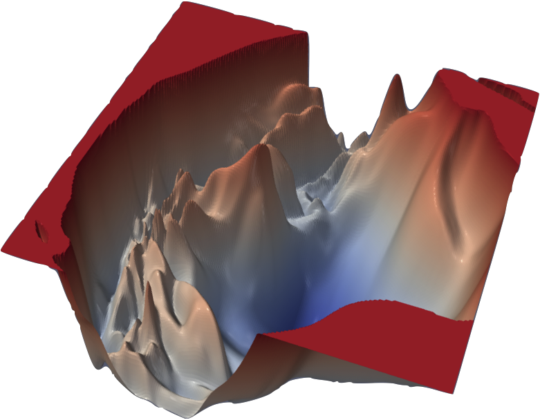
Conjecture V.2.

Consider a global minimum $\theta^{*}$, and two vectors $v_{1},v_{2}$ drawn by a certain rule (e.g. Gaussian distribution). Define the function

$$G_{v_{1},v_{2}}(\alpha,\beta)=F(\theta^{*}+\alpha v_{1}+\beta v_{2}),\alpha,\beta\in\mathbb{R}.$$

Then for standard neural nets with width above a threshold $c_{1}$, or ResNet with width above a threshold $c_{2}<c_{1}$, $G_{v_{1},v_{2}}(\alpha,\beta)$ has no sub-optimal basins. In addition, for standard neural-nets with width below a threshold $c_{1}^{\prime}<c_{1}$, $G_{v_{1},v_{2}}(\alpha,\beta)$ has many basins.

Theorem IV.2 and Proposition IV.3 discussed earlier (appeared in [32]) show a distinction between narrow and wide networks, thus have a similar flavor to Conjecture V.2. Nevertheless, it is unknown whether the original version of Conjecture V.2 can be proved.

Figure 5: Figure from [33] visualizing the landscape of ResNet-56 with different width. From left to right, the width is 1, 2, 4, 8 times as large as the original ResNet-56. The test error are $13.31\%$, $10.26\%$, $9.69\%$, $8.70\%$. Source: reprinted from [33].

V-B Mode connectivity

In this subsection, we present another interesting empirical finding, supported by some theoretical results. Draxler et al. [15] and Garipov et al. [18] empirically found that two global minima can be connected by an (almost) equal-value path. This means that the “modes” (meaning different global minima) are connected via equal-value path, which explains the terminology “mode connectivity”. We provide a formal description below.

Define $M(v_{1},v_{2},v_{3})$ as the linear space spanned by $v_{i},i=1,2,3$ for any three vectors $v_{1},v_{2},v_{3}$ (assuming linearly independent). Reference [18] generated Figure 6 (left part) as follows: first, train a standard 164-layer ResNet to find three solutions $\theta_{i}^{*},i=1,2,3$ by starting from three random initial points; second, define a function $f(s,t)=F(s\theta_{1}+t\theta_{2}+(1-s-t)\theta_{3})$, where $s,t\in\mathbb{R}$; third, draw the contour of the function $f(s,t)$ for $s,t$ in certain intervals. Note that we can interpret the three solutions as three global minima, even though they are not exact global minima. The plot shows that the three solutions lie at the bottom of three basins, thus we can make the following conjecture.

Conjecture V.3.

Suppose $\theta_{i}^{*},i=1,2,3$ are three global minima of $F$. Then in any continuous path in the plane $M(\theta_{1}^{*},\theta_{2}^{*},\theta_{3}^{*})$ that connects $\theta_{1}^{*}$ and $\theta_{2}^{*}$, the maximum of $F$ is strictly larger than $F(\theta_{1}^{*})$.

To understand whether $\theta_{1}^{*}$ and $\theta_{2}^{*}$ are connected via some equal-value path, we can search over the space of paths. Figure 6 (right part) empirically showed that there exists a simple path that connects two global minima.

Conjecture V.4.

Suppose $\theta_{1}^{*}$ and $\theta_{2}^{*}$ are two global minima of $F$. There exists $\theta_{0}$ such that the following holds: there exists a continuous path in the plane $M(\theta_{1}^{*},\theta_{2}^{*},\theta_{0})$ that connects $\theta_{1}^{*}$ and $\theta_{2}^{*}$ and passes $\theta_{0}$, along which the value of $F$ is constant.

In optimization language, mode connectivity means that the sub-level set $\{\theta\mid F(\theta)\leq F^{*}\}$, which is the same as $\{\theta\mid F(\theta)=F^{*}\}$, is connected, where $F^{*}$ is the global minimal value. These findings are partially motivated by Freeman and Bruna [17], who proved a stronger property that the sub-level set $\{\theta\mid F(\theta)\leq c\}$ is connected for any $c$, for deep linear networks and 1-hidden-layer ultra-wide ReLU networks. Kuditipudi et al. [29] and [42] provided a theoretical justification on this phenomenon; due to space limit, we do not discuss their results in detail.

Now we describe the empirical method used in [15] and [18] to verify mode connectivity. The goal is to find a equal-value path connecting two global-min. In practice it is hard to find exact global minima, thus a reasonable replacement is to train a neural-net to find two different solutions $\theta_{i}^{*},i=1,2$ by starting from two random initial points. To find a path $P$ connecting two points $\theta_{1}^{*}$ and $\theta_{2}^{*}$ with “equal-value”, these works use an optimization problem: find a path with the lowest “energy”, where the “energy” can be defined in different ways. [15] minimizes the “infinity-norm” of the path $P$, i.e., solve $\min_{P\text{ from }\theta_{1}^{*}\text{ to }\theta_{2}^{*}}\max_{\theta\in P}F(\theta)$, and [18] minimizes the “$\ell_{1}$-norm” of the path, i.e., solve $\min_{P\text{ from }\theta_{1}^{*}\text{ to }\theta_{2}^{*}}\mathbb{E}_{\theta}F(\theta)$, where $\theta$ is drawn from a certain random distribution on the path $P$.

We briefly discuss the practical tricks used in [18]. There is a huge number of continuous paths from $\theta_{1}^{*}$ to $\theta_{2}*$. To restrict the search space of the paths, it considers a subclass of paths, such as the class of Bezier curves $\theta_{\psi}(t)=(1-t)^{2}\theta^{*}_{1}+2t(1-t)\psi+t^{2}\theta^{*}_{2},t\in[0,1]$, where $\psi$ is any parameter. Then they use SGD to solve

$$\min_{\psi}E_{t\sim\text{U}[0,1]}F(\theta_{\psi}(t)).$$

The result is illustrated in Figure 6 (right part). The choice of Bezier curve is arbitrary, and they also report results of using other curves.

Figure 6: Figure from [18] illustrating mode connectivity. These are the contours of the loss of a 164-layer ResNet trained on CIFAR100, as a function of the network weights in a two-dimensional subspace. This subspace is spanned by the three points $\theta_{1}^{*},\theta_{2}^{*}$ (which are fixed) and $\psi$ (which can be changed). Here $\theta_{1}^{*},\theta_{2}^{*}$ are two solutions (likely local optima) found by training the network from two independent initial points. Left figure: $\psi$ is another solution found by training from another initial point, and we can see the barriers between the three minima. Right figure: $\psi$ is found by solving a problem, and we can see a quadratic Bezier curve connecting the two optima along a path of near-constant loss. Source: reprinted from [18].

Mode connectivity is not only an interesting geometrical finding, but has practical implications. For example, mode connectivity implies that once we find two global minima, there is likely to be a connected path between the two minima. This provides an opportunity for searching for better minima which yield lower test errors. In [18], such a technique has been proposed.

V-C Saddle points or local minima

An influential, early paper in the recent wave of landscape analysis by Dauphin et al [13] studied what points caused training difficulties. It advocated the hypothesis that saddle points instead of local minima are a major issue for neural network training. The underlying logic is the following: under the conjecture that most local minima are close to global minima, if an algorithm gets stuck at a point with a large error, then it is likely to be a saddle point instead of a local minimum. This claim is one of motivations for many later works on escaping saddle points (see Sec. VII-B). Whether saddle points or local minima are a more severe issue remains an interesting question.

VI Eliminating bad local minima for non-linear networks

We have discussed that eliminating sub-optimal local minima globally is difficult, thus we resort to more complicated concepts such as spurious valleys. In this section, we follow a different path: we still try to eliminate bad local minima, but allow the modification of other parts of the game. First, we discuss results that eliminate bad local minima in a subset but not the whole space. Second, we show how to force all local minima to fall into a subset so that no bad local-min exists. Third, we discuss the limitation of eliminating bad-min, and discuss a stronger landscape property and a result on it.

VI-A Eliminating bad local-min in a subset

Local minima with full-rank post-activation matrices. Reference [43, Theorem 3.4, 3.8] provided conditions for the absence of local-min with certain full-rank condition. Below we present a different version in [32]. Define $z_{0}(x)=x$ and $z_{k}(x)=\phi(W_{k-1}z_{k-1}(x)+b_{k}),$, $k=1,2,\dots,L$. Then we can write $f_{w}(x)=W_{L}Z_{L}(x)$. Let $X=(x_{1},\dots,x_{n})$ and let $Z_{L}(X)=(z_{L}(x_{1}),\dots,z_{L}(x_{n})).$

Claim VI.1.

Define $\mathcal{W}_{\rm L,full}=\{\theta:Z_{L}(X)\text{ is full rank}\}$. Every local minimum of $F(\theta)$ in the set $\mathcal{W}_{\rm L,full}$ is a global minimum.

Claim VI.2.

Suppose the $k$-th order derivative of the activation function $\sigma^{(k)}(0)$ are non-zero, for $k=0,1,2,\dots,n-1.$ Then the set $\mathcal{W}_{\rm L,full}$ is dense.

Claim VI.1 is of interest in its own since it is rather simple. The results discussed in Sec. IV-D can be viewed as more modern versions (with no restriction to a subset).

Local minima with full-rank NTK. There is another simple result of a similar flavor. For simplicity of presentation, we assume $d_{y}=1$. Define

$$G(\theta)=(\frac{\partial f_{\theta}(x_{1})}{\partial\theta},\dots,\frac{\partial f_{\theta}(x_{n})}{\partial\theta})\in\mathbb{R}^{P\times n}$$ (5)

where $P$ is the number of parameters, and define neural tangent kernel (NTK)

$$K(\theta)=G(\theta)^{T}G(\theta).$$ (6)

Claim VI.3.

Suppose $d_{y}=1$ and $\ell(a,b)=(a-b)^{2}.$ Define $\mathcal{W}_{\rm NTK}=\{\theta:K(\theta)\text{ is full rank}\}$. Every critical point $\theta^{*}$ of $F(\theta)$ in the set $\mathcal{W}_{\rm NTK,full}$ is a global minimum with zero value.

Proof: Let $e_{i}^{*}=f_{\theta^{*}}(x_{i})-y_{i}$ and $e^{*}=(e_{1}^{*};\dots;e_{n}^{*})\in\mathbb{R}^{n\times 1}$. Since $F(\theta)=\frac{1}{n}\sum_{i=1}^{n}(y_{i}-f_{\theta}(x_{i}))^{2},$ we have

$$\frac{dF(\theta^{*})}{d\theta}=\frac{2}{n}G(\theta^{*})e^{*}.$$

If $\frac{dF(\theta^{*})}{d\theta}=0$ and $G(\theta^{*})$ is full rank, we have $e^{*}=0$ and thus $F(\theta^{*})=0$, implying $\theta^{*}$ is a global-min. Q.E.D.

Full-rankness of $G(\theta)$ is equivalent to the full-rankness of $K(\theta)$; we do not need $K(\theta)$ here but we still define $K(\theta)$ since it is critical in NTK theory. Despite simplicity, Claim VI.3 can be viewed as the foundation of the NTK theory we discussed later.

Local minima with an inactive neuron. The idea of considering local minima with special structure dates back to at least the classical work on Burer-Monteiro factorization [9]. It showed that for a certain class of non-convex matrix problem, a local-min with a zero column must be a global-min. This result is not directly related to neural nets, but it indicated an interesting direction.

Reference [20] analyzed a two-layer neural network $W_{2}\phi(W_{1}x)$ with positive homogeneous activations (e.g. ReLU, linear). It proved that a local-min with one inactive neuron is a global-min (a formal result is somewhat technical and omitted here). Note that the optimization variables are the two weight matrices $W_{1}$ and $W_{2}$, thus “an inactive neuron” means that there is an index $j$ such that the $j$-th row of $W_{1}$ and $W_{2}^{\top}$ are both zero. This can be viewed as a variant of the result of [9].

Comments. Eliminating bad local-min in a subset itself is of limited interest, since an algorithm may or may not stay in this subset. Extra techniques are required to make these results more interesting. The three results we presented in this subsection are indeed extended to three stronger results ( Theorem IV.2, NTK theory [23] and Theorem VI.2 respectively). Again, we present them here since they are simple and provide some insight.

VI-B Making modifications to eliminate bad local-min

Eliminating bad local-min by ensuring an inactive neuron.

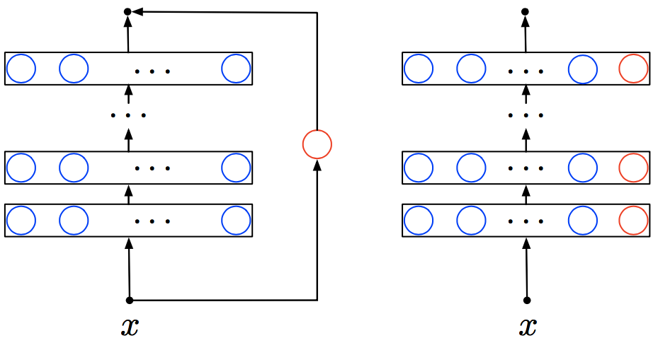
A recent work [36] proved that by slightly modifying the neural network and adding a regularizer, every local minimum is a global minimum. This can be viewed as an extension of the line of works on local minima with special sparse structure [9, 20] as a key idea is to force all local minima to exhibit the special structure. Reference [36] provides two modifications of the system, each of which can ensure no bad local-min exists, for binary classification. In the first modification, for any deep neural network, [36] added a special neuron (e.g. exponential) from input to output and a quadratic regularizer on its weight. The second modification is to use a special neuron (e.g. exponential) at each layer and add regularizers for the weights connected to these special neurons. The two modifications are demonstrated in Figure 7.

Below we present the result for the first modification [36, Theorem 1]. Assume that there exists a $\bm{\theta}$ such that the neural net $f_{\theta}$ can correctly classify all samples in the dataset. Now we add an exponential neuron to the architecture and have a modified function $\tilde{f}(x;\tilde{\bm{\theta}})=f_{\bm{\theta}}(x)+a\exp(\bm{w}^{\top}x+b)$. For the logistic loss function $\ell(y,z)=\log_{2}(1+e^{-yz})$, we consider a modified loss function

$$\tilde{L}_{n}(\tilde{\bm{\theta}})=\sum_{i=1}^{n}\ell\left(y_{i},\tilde{f}(x;\tilde{\bm{\theta}})\right)+\frac{\lambda a^{2}}{2}.$$ (7)

The original loss function is defined as

$$L_{n}(\tilde{\bm{\theta}})=\sum_{i=1}^{n}\ell\left(y_{i},f_{\bm{\theta}}(x_{i}))\right).$$

Theorem VI.1.

([36, Theorem 1]) Under the above settings, we have:

• The function $\tilde{L}_{n}(\tilde{\bm{\theta}})$ has at least one local minimum.

• At every local minimum, $a=0$.

• Assume that $\tilde{\bm{\theta}}^{*}=(\bm{\theta}^{*},a^{*},\bm{w}^{*},b^{*})$ is a local minimum of $\tilde{L}_{n}(\tilde{\bm{\theta}})$, then $\tilde{\bm{\theta}}^{*}$ is a global minimum of $\tilde{L}_{n}(\tilde{\bm{\theta}})$. Furthermore, $\bm{\theta}^{*}$ achieves the minimum loss value on the dataset $\mathcal{D}$, i.e., $\bm{\theta}^{*}\in\arg\min_{\bm{\theta}}{L}_{n}(\bm{\theta})$.

The proof consists of two steps. [36] first showed that at any critical point of the loss function, the exponential neuron is always inactive. This trick allows us to consider local-min in a subset (the topic of the previous subsection). Then [36] proved that a local-min with an inactive neuron is a global-min.

Figure 7: Figure from [36] illustrating the modifications. On the left, a special neuron (e.g. exponential) is added from input to output. On the right, there architecture is a regular fully connected neural network, and at each layer there is a special neuron (e.g. exponential). Source: reprinted from [36].

Extension to multi-class classification and regression. Reference [26] extends [36] (the first modification) to the multi-class classification tasks. Similar to the construction proposed by [36], it added an exponential neuron on the output of the neural network for each class and added an $\ell_{2}$ regularizer for the parameters of all exponential neurons. The high-level proof ideas adopted those of [36] (though with some technical differences). It first showed that at every local minimum of the empirical loss function, all exponential neurons are inactive. Then it showed that a local-min with these neurons inactive must be a global-min.

Limitation of eliminating bad local-min. [36, 26] showed that it is not difficult to prove every local-min is a global-min as long as small modifications can be made. However, [26] argued that there are simple examples where on the modified landscape, there are new paths leading the original local-min to infinity, and thus a descent algorithm might diverge to infinity. We remark that most works on landscape analysis of neural networks mentioned earlier do not explicitly eliminate the possibility that a descent algorithm will diverge to infinity. For instance, for a 3-layer 1-dimensional linear network problem $\min_{x,y,z\in\mathbb{R}}(xyz-1)^{2}$, although no sub-optimal local-min exists according to [25], there is a sequence $(x_{k},y_{k},z_{k})=(-1/k,\sqrt{k},1/k)$ diverging to infinity while the function values are decreasing and converging to $1$, which is clearly a sub-optimal value. This shows that a “decreasing path” to infinity exists even for linear neural networks.

VI-C Eliminating bad local-min and decreasing path to infinity

A natural question is then whether one can further eliminate the possibility of decreasing path to infinity as well as sub-optimal local-min. All the results we discussed so far cannot satisfy both properties together. Some results prove no sub-optimal local-min [25, 36, 37, 26], but their loss functions may have decreasing path to infinity.

Reference  [38] provides a positive answer to the question. [38] considers over-parameterized neural-nets with arbitrary depth. For simplicity of presentation, we state their result for a 1-hidden-layer network. This network can be expressed by $f(x;\bm{\theta})=\sum_{j=1}^{m}a_{j}\text{ReQU}\left(\bm{w}_{j}^{\top}x+b_{j}\right),$ where the scalar $a_{j}$, vector $\bm{w}_{j}$, scalar $b_{j}$ denote the coefficient, weight vector, bias of the $j$-th neuron and $w_{j}$’s) in the neural network and the activation function is $\text{ReQU}(z)=[\max\{z,0\}]^{2}$. Suppose the loss function is logistic: $\ell(y;z)=\log(1+e^{-yz})$. Furthermore, reference [38] assumes that the data points $x_{1},\dots,x_{n}$ are distinct. The loss to minimize is

$$\begin{split}F(\bm{\theta})&=\sum_{i=1}^{n}\ell(y_{i};f(x_{i};\bm{\theta}))+\\ &\frac{1}{3}\sum_{j=1}^{m}\lambda_{j}\left[|a_{j}|^{3}+2\left(\|\bm{w}_{j}\|^{2}_{2}+b_{j}^{2}\right)^{3/2}\right],\end{split}$$ (8)

where all regularizer coefficients $\lambda_{j}$’s are positive numbers and the vector $\bm{\lambda}=(\lambda_{1},...,\lambda_{m})$ consists of all regularizer coefficients. [38] shows that if the network size is larger than the dataset size, i.e., $m\geq n+1$ and the regularizer coefficient vector $\bm{\lambda}$ is chosen in a specific way, then every local-min achieves zero training error. In this result, we use a standard notion called “coercive”: we say $F$ is a coercive function iff $\lim_{\|\theta\|\rightarrow\infty}F(\theta)=\infty$, thus a coercive function has no decreasing path to infinity.

Theorem VI.2.

Let $m\geq n+1$. There exists a $\lambda_{0}=\lambda_{0}(\mathcal{D},\ell)>0$ and a zero measure set $\mathcal{C}\subset\mathbb{R}^{m}$ such that for any $\bm{\lambda}\in(0,\lambda_{0})^{m}\setminus\mathcal{C}$, both of the following statements are true:

• The empirical loss $F(\bm{\theta})$ is coercive.

• Every local minimum $\bm{\theta}^{*}$ of the loss $F(\bm{\theta})$ is a global minimum of $F(\bm{\theta})$, and achieves zero training error.

Remark: When all data points are distinct and the size of the ReQU network is larger than the size of the dataset, it is straightforward to show that the every sample in the dataset can be correctly classified by the neural network. In other words, there exists $\theta^{*}$ such that $F(\theta^{*})=0$. This fact is commonly known as “over-parameterization implies interpolation”.

The limitation of the result is that it considers a special neuron called ReQU. Nevertheless, this result at least shows the possibility of achieving both “no bad local-min” and “no decreasing path to infinity”.

VII Algorithmic Analysis

As mentioned in the introduction, although algorithmic analysis is very important and closely related to optimization landscape, it is not the focus of this short article. Nevertheless, we briefly discuss convergence analysis for a better big picture.

VII-A Intuition: Avoiding Bad Regions

For a landscape with no bad basin (discussed in Sec. IV-D), we expect the training is easier than a landscape with bad basins. Intuitively, without bad basins, global minima are the major attractors for SGD (local-min can only attract a tiny subset of points), thus starting from a random initial point the optimization trajectory will converge to global minima with high probability. See Figure 8 for a conceptual illustration of the global landscape: bad regions exist, but are rare. We formalize this notion of “good landscape” below.

Definition VII.1.

For a given deterministic algorithm $\mathcal{A}$ that maps a point $\theta$ to $\mathcal{A}(\theta)$, define $\phi_{\mathcal{A}}(\theta)=\liminf_{k\rightarrow\infty}F(\mathcal{A}^{k}(\theta))$.

Conjecture VII.1.

(informal) Suppose the neural net has $O(n)$ parameters and the input data are generic. Consider an algorithm $\mathcal{A}(\theta)=\theta-\eta\nabla F(\theta)$. For a proper constant $\eta$, and for a random initial point drawn from a certain distribution (e.g. Xavier initialization), $\text{Pr}(\phi_{\mathcal{A}}(\theta)<\epsilon)>1-\delta,$ where $\epsilon,\delta$ are certain small constants.

Currently there is a gap between the landscape results and the above conjecture. Although landscape results provide positive evidence for the conjecture, we may need to utilize extra properties of the neural-nets to prove the conjecture.

Figure 8: Illustration of a landscape where bad regions (starting from where GD will end up at highly sub-optimal values) occupy a small portion. Bad regions are hard to escape, but they can be avoided for most initial points. For neural-net problems, the loss landscape is more complicated than this figure, but we suspect that a similar claim holds: bad regions occupy a small portion. Results like “No bad basin or spurious valley” provide evidence for this claim, but are not enough to prove it.

Adding noise to GD can further increase the probability of success, since shallow basins can potentially be escaped with noise. There is another perspective (e.g. [28, 50]) on the benefit of noise: running SGD for a function can be seen as running GD for a “smoothed function”. Shallow local-min of the original function may disappear in the “smoothed landscape”. Nevertheless, [28, 50] only studied special shallow networks. A general analysis of deep neural-nets using this perspective is still missing.

VII-B Escaping Bad Points

We distinguish two methods for proving convergence of an algorithm to global-min.

• Avoidance-method: for most initial points the algorithm can avoid bad regions along the trajectory, thus converging to global-min.

• Escape-method: for almost all initial points the algorithm can escape bad regions, thus converging to global-min.

Figure 8 provides an example where the avoidance-method can succeed but the escape-method fails: there is a positive measure of bad region that GD will get stuck, but for most initial points GD avoids this bad region.

The escape-method has been used in matrix optimization to prove convergence to global-min (see [10]). A usual pipeline is: first, prove no sub-optimal local-min exists; second, prove every saddle point is a strict saddle point (critical point whose Hessian has at least one negative eigenvalue); third, noisy GD converges to a global-min based on general results in, e.g, [31],[24].

For neural-nets, a theoretical challenge is that high-order saddle points (a saddle point that is not a strict saddle point) may exist. Reference [4] showed that escaping fourth-order or higher-order saddle points is NP-hard. Therefore, to prove a rigorous convergence result of GD, just proving “no bad local-min” is not enough for general non-convex problems.

That being said, for over-parameterized neural-nets, it is possible that the trajectory did not pass a saddle point since saddle points can only attract a tiny portion of initial points (as Conjecture VII.1 states). A more promising approach towards convergence to global minima seems to be the avoidance-method. We discuss some results related to the avoidance-method in the next subsection.

VII-C Algorithmic Analysis for Ultra-Wide Networks

One way of implementing the avoidance-method is the following two-step approach: (a) prove that in a subset of the parameter space every local-min is a global-min; (b) prove that under certain conditions the optimization trajectory stays in this subset.

Consider the NTK Gram matrix $K(\theta)=G(\theta)^{T}G(\theta)$, where $G(\theta)=(\frac{\partial f_{\theta}(x_{1})}{\partial\theta},\dots,\frac{\partial f_{\theta}(x_{n})}{\partial\theta})$, assuming $d_{y}=1$.

Claim VII.1.

Suppose the conditions of Claim VI.3 hold. Suppose a certain algorithm generates a sequence $\theta(k+1)=\mathcal{A}(\theta(k)),k=0,1,2,\dots,$ where $\mathcal{A}$ is a continuous mapping. Assume there exists $c>0$ such that $\lambda_{\min}(G(\theta(k)))\geq c,\forall k$, where $\lambda_{\min}$ indicates the smallest eigenvalue. Assume a limit point $\theta^{*}$ of the sequence $\{\theta(k)\}$ is a critical point of $F(\theta)$, then $\theta^{*}$ is a global minimum of $F(\theta)$ with zero value.

Proof: Since $\mathcal{A}$ is continuous, the limit point of the sequence $\{\theta(k)\}$ also satisfies $\lambda_{\min}(G(\theta^{*}))\geq c$. According to Claim VI.3, $\theta^{*}$ is a global-min of $F(\theta)$ with zero value. Q.E.D.

Recent works [23, 6, 30] prove that with infinite width (or $poly(n)$ neurons per layer), $K(\theta)$ stays positive-definite along the trajectory of GD with a random initialization, thus finishing the a key step of the convergence proof. The power of the NTK framework is not just proving convergence, but also linear convergence rate, and even generalization error bound. These aspects are beyond the scope of this article, so will not be discussed in detail here. Around the same time as [23], references [52, 16, 2] also prove global convergence of gradient descent under similar “ultra-wide” condition; we skip the details of these results here.

Despite the strong conclusions (convergence, convergence rate, etc.), the assumption of a large width in these convergence results (often a polynomial of $n$, at least $\Omega(n^{2})$) is not satisfied by practical neural nets. Nevertheless, a more important aspect is the theoretical insight. An intuition of NTK theory is that for extremely wide networks, the weights have little change during the whole training procedure, and hence the model behaves as its linearization around the initialization. However, reference [11] showed by experiments that the dynamics of the linearized networks is different from the practical training dynamics, thus the existing results based on NTK may not be enough to fully explain the practical training.

When the theory does not fully match practice, we do not necessarily have to modify theory; we can also modify the practical system (as mentioned in Q3 in the introduction). [23] suggested that one could use kernel GD with the kernel being the NTK to solve machine learning problems. This essentially reduces a complex multi-layer non-linear network to a simple linear model. We stress that this is a new method, and is different from practical training. [6] performed precise computation using kernel GD with NTK, and reported promising results on image classification. One possible issue is that kernel GD is much slower than training a neural net due to high dimension (at least for now).

A convergence result with all assumptions being practical (using common gradient descent; arbitrary depth; not too large width; mild data assumption) is still unknown. Convergence analysis of neural-nets (including but not limited to NTK-type analysis) is a very active area of research (besides the aforementioned works, see, e.g., [3, 5, 34, 22, 1]). It probably requires another whole article to fully review the recent advances. The focus of this article is on the geometric side of neural-nets, as mentioned in the introduction, thus we do not go deeper into convergence analysis.

VIII Conclusion

In this article, we reviewed recent progress on the understanding of the global landscape of neural networks. We discussed various empirical findings on the landscape, and also many theoretical results. We first reviewed the results on deep linear networks that no bad local-min exists. We then discussed why a classical claim on “no bad local-min” for over-parameterized networks fails to hold, and showed that a more rigorous claim should be no spurious valley (or no bad basin). We discussed how to perturb the loss functions to eliminate bad local-min, the limitation of “no bad local-min”, and how to obtain a stronger landscape property. Finally, we briefly discussed the existing convergence analysis (especially NTK).

While the progress is encouraging, there are still many mysteries on the landscape of neural-nets. Many questions presented in this article are not answered (search “Conjecture” or “open” to find them). How to leverage the insight obtained from the theory to design better methods/architectures is also an interesting question.

References

- [1] Z. Allen-Zhu, Y. Li, and Y. Liang. Learning and generalization in overparameterized neural networks, going beyond two layers. In Advances in neural information processing systems, pages 6158–6169, 2019.
- [2] Z. Allen-Zhu, Y. Li, and Z. Song. A convergence theory for deep learning via over-parameterization. In International Conference on Machine Learning, pages 242–252, 2019.
- [3] Z. Allen-Zhu, Y. Li, and Z. Song. On the convergence rate of training recurrent neural networks. In Advances in Neural Information Processing Systems, pages 6673–6685, 2019.
- [4] A. Anandkumar and R. Ge. Efficient approaches for escaping higher order saddle points in non-convex optimization. In Conference on learning theory, pages 81–102, 2016.
- [5] S. Arora, S. Du, W. Hu, Z. Li, and R. Wang. Fine-grained analysis of optimization and generalization for overparameterized two-layer neural networks. In International Conference on Machine Learning, pages 322–332, 2019.
- [6] S. Arora, S. S. Du, W. Hu, Z. Li, R. R. Salakhutdinov, and R. Wang. On exact computation with an infinitely wide neural net. In Advances in Neural Information Processing Systems, pages 8139–8148, 2019.
- [7] P. Baldi and K. Hornik. Neural networks and principal component analysis: Learning from examples without local minima. Neural networks, 2(1):53–58, 1989.
- [8] M. Bianchini and M. Gori. Optimal learning in artificial neural networks: A review of theoretical results. Neurocomputing, 13(2-4):313–346, 1996.
- [9] S. Burer and R. D. Monteiro. A nonlinear programming algorithm for solving semidefinite programs via low-rank factorization. Mathematical Programming, 95(2):329–357, 2003.
- [10] Y. Chi, Y. M. Lu, and Y. Chen. Nonconvex optimization meets low-rank matrix factorization: An overview. IEEE Transactions on Signal Processing, 67(20):5239–5269, 2019.
- [11] L. Chizat, E. Oyallon, and F. Bach. On lazy training in differentiable programming. In Advances in Neural Information Processing Systems, pages 2933–2943, 2019.
- [12] A. Choromanska, M. Henaff, M. Mathieu, G. B. Arous, and Y. LeCun. The loss surfaces of multilayer networks. In Artificial Intelligence and Statistics, pages 192–204, 2015.
- [13] Y. N. Dauphin, R. Pascanu, C. Gulcehre, K. Cho, S. Ganguli, and Y. Bengio. Identifying and attacking the saddle point problem in high-dimensional non-convex optimization. In Advances in neural information processing systems, pages 2933–2941, 2014.
- [14] T. Ding, D. Li, and R. Sun. Sub-optimal local minima exist for almost all over-parameterized neural networks. arXiv preprint arXiv:1911.01413, 2019.
- [15] F. Draxler, K. Veschgini, M. Salmhofer, and F. Hamprecht. Essentially no barriers in neural network energy landscape. In International Conference on Machine Learning, pages 1309–1318, 2018.
- [16] S. Du, J. Lee, H. Li, L. Wang, and X. Zhai. Gradient descent finds global minima of deep neural networks. In International Conference on Machine Learning, pages 1675–1685, 2019.
- [17] C. D. Freeman and J. B. Estrach. Topology and geometry of half-rectified network optimization. In International Conference on Learning Representations, 2017.
- [18] T. Garipov, P. Izmailov, D. Podoprikhin, D. P. Vetrov, and A. G. Wilson. Loss surfaces, mode connectivity, and fast ensembling of dnns. In Advances in Neural Information Processing Systems, pages 8789–8798, 2018.
- [19] I. J. Goodfellow, O. Vinyals, and A. M. Saxe. Qualitatively characterizing neural network optimization problems. arXiv preprint arXiv:1412.6544, 2014.
- [20] B. D. Haeffele and R. Vidal. Global optimality in neural network training. In Proceedings of the IEEE Conference on Computer Vision and Pattern Recognition, pages 7331–7339, 2017.
- [21] S. Han, H. Mao, and W. J. Dally. Deep compression: Compressing deep neural networks with pruning, trained quantization and huffman coding. arXiv preprint arXiv:1510.00149, 2015.
- [22] J. Howard. Now anyone can train Imagenet in 18 minutes. https://www.fast.ai/2018/08/10/fastai-diu-imagenet/, 2018.
- [23] A. Jacot, F. Gabriel, and C. Hongler. Neural tangent kernel: Convergence and generalization in neural networks. In Advances in neural information processing systems, pages 8571–8580, 2018.
- [24] C. Jin, R. Ge, P. Netrapalli, S. M. Kakade, and M. I. Jordan. How to escape saddle points efficiently. In Proceedings of the 34th International Conference on Machine Learning-Volume 70, pages 1724–1732. JMLR. org, 2017.
- [25] K. Kawaguchi. Deep learning without poor local minima. In Advances in neural information processing systems, pages 586–594, 2016.
- [26] K. Kawaguchi and L. P. Kaelbling. Elimination of all bad local minima in deep learning. arXiv preprint arXiv:1901.00279, 2019.
- [27] N. S. Keskar, D. Mudigere, J. Nocedal, M. Smelyanskiy, and P. T. P. Tang. On large-batch training for deep learning: Generalization gap and sharp minima. arXiv preprint arXiv:1609.04836, 2016.
- [28] B. Kleinberg, Y. Li, and Y. Yuan. An alternative view: When does sgd escape local minima? In International Conference on Machine Learning, pages 2698–2707, 2018.
- [29] R. Kuditipudi, X. Wang, H. Lee, Y. Zhang, Z. Li, W. Hu, R. Ge, and S. Arora. Explaining landscape connectivity of low-cost solutions for multilayer nets. In Advances in Neural Information Processing Systems, pages 14574–14583, 2019.
- [30] J. Lee, L. Xiao, S. Schoenholz, Y. Bahri, R. Novak, J. Sohl-Dickstein, and J. Pennington. Wide neural networks of any depth evolve as linear models under gradient descent. In Advances in neural information processing systems, pages 8572–8583, 2019.
- [31] J. D. Lee, M. Simchowitz, M. I. Jordan, and B. Recht. Gradient descent only converges to minimizers. In Conference on learning theory, pages 1246–1257, 2016.
- [32] D. Li, T. Ding, and R. Sun. On the benefit of width for neural networks: Disappearance of bad basins. arXiv preprint arXiv:1812.11039, 2018.
- [33] H. Li, Z. Xu, G. Taylor, C. Studer, and T. Goldstein. Visualizing the loss landscape of neural nets. In Advances in Neural Information Processing Systems, pages 6391–6401, 2018.
- [34] Y. Li and Y. Liang. Learning overparameterized neural networks via stochastic gradient descent on structured data. In Advances in Neural Information Processing Systems, pages 8157–8166, 2018.
- [35] Y. Li, T. Ma, and H. Zhang. Algorithmic regularization in over-parameterized matrix sensing and neural networks with quadratic activations. In Conference On Learning Theory, pages 2–47, 2018.
- [36] S. Liang, R. Sun, J. D. Lee, and R. Srikant. Adding one neuron can eliminate all bad local minima. In Advances in Neural Information Processing Systems, pages 4355–4365, 2018.
- [37] S. LIANG, R. Sun, Y. Li, and R. Srikant. Understanding the loss surface of neural networks for binary classification. In International Conference on Machine Learning, pages 2835–2843, 2018.
- [38] S. Liang, R. Sun, and R. Srikant. Revisiting landscape analysis in deep neural networks: Eliminating decreasing paths to infinity. arXiv preprint arXiv:1912.13472, 2019.
- [39] H. Lu and K. Kawaguchi. Depth creates no bad local minima. arXiv preprint arXiv:1702.08580, 2017.
- [40] Y. Nesterov and V. Spokoiny. Random gradient-free minimization of convex functions. Foundations of Computational Mathematics, 17(2):527–566, 2017.
- [41] B. Neyshabur. Implicit regularization in deep learning. arXiv preprint arXiv:1709.01953, 2017.
- [42] Q. Nguyen. On connected sublevel sets in deep learning. In International Conference on Machine Learning, pages 4790–4799, 2019.
- [43] Q. Nguyen and M. Hein. The loss surface of deep and wide neural networks. In International Conference on Machine Learning, pages 2603–2612, 2017.
- [44] Q. Nguyen, M. C. Mukkamala, and M. Hein. On the loss landscape of a class of deep neural networks with no bad local valleys. In International Conference on Learning Representations, 2019.
- [45] I. Safran and O. Shamir. Spurious local minima are common in two-layer relu neural networks. In International Conference on Machine Learning, pages 4433–4441, 2018.
- [46] R.-Y. Sun. Optimization for deep learning: An overview. Journal of the Operations Research Society of China, 2019.
- [47] L. Venturi, A. Bandeira, and J. Bruna. Neural networks with finite intrinsic dimension have no spurious valleys. arXiv preprint arXiv:1802.06384, 15, 2018.
- [48] X. Yu and S. Pasupathy. Innovations-based MLSE for Rayleigh flat fading channels. IEEE Transacations on Communications, pages 1534–1544, 1995.
- [49] C. Yun, S. Sra, and A. Jadbabaie. Global optimality conditions for deep neural networks. In International Conference on Learning Representations, 2018.
- [50] M. Zhou, T. Liu, Y. Li, D. Lin, E. Zhou, and T. Zhao. Towards understanding the importance of noise in training neural networks. arXiv preprint arXiv:1909.03172, 2019.
- [51] Y. Zhou and Y. Liang. Critical points of neural networks: Analytical forms and landscape properties. In International Conference on Learning Representations, 2018.
- [52] F. Zou, L. Shen, Z. Jie, J. Sun, and W. Liu. Weighted adagrad with unified momentum. arXiv preprint arXiv:1808.03408, 2018.