Active Control and Sustained Oscillations
in actSIS Epidemic Dynamics

Abstract

An actively controlled Susceptible-Infected-Susceptible (actSIS) contagion model is presented for studying epidemic dynamics with continuous-time feedback control of infection rates. Our work is inspired by the observation that epidemics can be controlled through decentralized disease-control strategies such as quarantining, sheltering in place, social distancing, etc., where individuals actively modify their contact rates with others in response to observations of infection levels in the population. Accounting for a time lag in observations and categorizing individuals into distinct sub-populations based on their risk profiles, we show that the actSIS model manifests qualitatively different features as compared with the SIS model. In a homogeneous population of risk-averters, the endemic equilibrium is always reduced, although the transient infection level can exhibit overshoot or undershoot. In a homogeneous population of risk-tolerating individuals, the system exhibits bistability, which can also lead to reduced infection. For a heterogeneous population comprised of risk-tolerators and risk-averters, we prove conditions on model parameters for the existence of a Hopf bifurcation and sustained oscillations in the infected population.

1 Introduction

Deterministic compartmental models in epidemiology have provided valuable insights for the understanding of evolutionary dynamics of infectious disease spread in a host population (Kermack and McKendrick (1927)). These models have also been widely applied to study various other spreading dynamics, including but not limited to information dissemination in social networks (Jin et al. (2013)), sentiment contagion in human society (Zhao et al. (2014)) and the propagation of systemic risks in financial market (Demiris et al. (2014)). Although these deterministic models unavoidably ignore some important details such as individual heterogeneity and network structure, they adequately capture the qualitative features of the spreading dynamics, including transient system behavior and stability of solutions. The models have been shown to be close approximations of certain Markov chain models of the underlying stochastic dynamics, see, e.g., Sahneh et al. (2013). The Susceptible-Infected-Susceptible (SIS) model has been widely studied and applied in epidemiological modeling. While its assumption that individuals acquire no immunity after recovery may not be suitable for certain diseases, it provides a worst case scenario, which is valuable for a large class of contagious diseases in general.

The SIS model in its simplest form assumes a constant infection rate. However, it is well acknowledged that the rate can vary over time due to the different control strategies taken by individuals, which in turn affects the contagion dynamics. Indeed, understanding such models and their extensions is fundamental to developing disease control strategies. A review of analysis and control of epidemics is provided in Nowzari et al. (2016).

In this paper, we propose a model with feedback controlled infection rates to account for active control strategies. Individuals modify their contact rates with others based on what they observe about the level of infection in the population. We model a time lag in the observations and distinguish individuals as risk-averters, risk-tolerators, and risk-ignorers. Risk-averters represent those who change their contact rate with others in the opposite direction as the change in the observed infected population level, e.g., those who could and did stay at home and practiced increased social distancing during the COVID-19 pandemic as they saw the infected population grow. Risk-tolerators represent those whose contact rate with others changes in the same direction as the change in the observed infected population level, e.g., health care workers, delivery workers, and other essential workers, who were obliged to work during the COVID-19 pandemic. Risk-ignorers represent those who do not actively modify their contact rates.

Our work contributes to the literature in the following ways. First, while active and passive spreading was first distinguished in the social economics literature (see Hartmann et al. (2008)), our model rigorously demonstrates the differences between them, and we prove new results on the dynamics of contagion with active control. Further, our model serves as one form of the state-dependent approaches discussed in Rands (2010) that offer evolutionarily grounded ways for studying social contagion in collective processes. Second, our feedback model uses a low-pass filter of the measured infected population level. This models the observation delay and introduces an important robustness to uncertainty. This is in contrast to contagion models which feed back infected population level directly, as in Baker (2020); Franco (2020). Third, we prove a new and relatively simple scenario under which sustained oscillations appear within epidemiological frameworks without external forcing. Understanding mechanisms that can lead to oscillations is critically important in the context of infectious disease spread (Lin et al. (1999); Dushoff et al. (2004); Camacho et al. (2011), Xu et al. (2020)). It is likewise of great interest in many other socio-economic processes, e,g., the rise and fall of business cycles (Mishchenko (2014)) and fluctuation of behavioral preferences in social networks (Pais et al. (2012)). Fourth, in contrast to control strategies that require global knowledge about the exact underlying spreading dynamics, e.g., Nowzari et al. (2016), our work provides evidence for the promise of tunable decentralized active control strategies to manage the dynamics of epidemics.

The paper is organized as follows. In Section 2, we review the Susceptible-Infected-Susceptible (SIS) model. We introduce the actively controlled Susceptible-Infected-Susceptible (actSIS) model in homogeneous populations of risk-tolerators and risk-averters respectively in Section 3, where we analyze the equilibrium solutions and stability conditions and show their qualitatively different features as compared with the SIS model. We examine the actSIS model in a heterogeneous population comprised of risk-tolerators and risk-averters in Section 4, and prove conditions for a Hopf bifurcation with a stable limit cycle. We conclude in Section 5.

2 Background

2.1 SIS in a well-mixed population

Consider a disease spreading in a large, randomly-mixed population, where individuals are divided into either susceptible (S) or infected (I) classes. Susceptible individuals get infected at rate $\beta$ while infected individuals recover at rate $\delta$. Let $p(t)$ be the fraction of infected individuals and $s(t)$ the fraction of susceptible individuals at time $t$. The SIS model is

$$\dot{s}=-\beta sp+\delta p,\;\;\;\dot{p}=\beta sp-\delta p.$$ (1)

The force of infection term $\beta p$ in (1) describes the rate at which susceptible individuals get infected (Muench (1934)). It can be decomposed into three terms: $\beta p=\bar{\beta}\times\alpha\times p$, where $\bar{\beta}$ is the transmission rate of the disease and an intrinsic property of the disease, and $\alpha$ is the effective number of contacts per unit time. Since $s(t)=1-p(t)$, (1) can be rewritten as

$$\dot{p}=\beta\left(1-p\right)p-\delta p.$$ (2)

The steady-state behavior of solutions to the well-mixed SIS model (2) is characterized by the basic reproduction number $\mathcal{R}_{0}=\beta/\delta$, a key concept in epidemiology that defines the epidemic threshold of a particular infection (Diekmann et al. (1990)). If $\mathcal{R}_{0}>1$, the disease persists and a nonzero fraction of the population is infected at steady state: as $t\rightarrow\infty$, $p(t)\rightarrow 1-\delta/\beta$, the endemic equilibrium (EE). If $\mathcal{R}_{0}\leq 1$, the disease dies out at steady state: as $t\rightarrow\infty$, $p(t)\rightarrow 0$, the infection free equilibrium (IFE). At $\mathcal{R}_{0}=1$, there is a transcritical bifurcation.

2.2 Network SIS model

A natural extension of the homogeneous population setting is the introduction of heterogeneities of various kinds. Characterizing population heterogeneity in terms of infection and/or recovery rates has been discussed both in population subgroups (Anderson and May (1992)) and in networks (Hethcote and Yorke (1984), Pagliara and Leonard (2020)). In the following, we review the network SIS model that was originally introduced as the multi-group SIS model in Lajmanovich and Yorke (1976).

Consider a heterogeneous population of $n$ sub-populations, each large, well-mixed and homogeneous. Let susceptible individuals in sub-population $i$ get infected through contact with infected individuals in sub-population $j$ at rate $\beta_{ij}\geq 0$ and infected individuals in sub-population $i$ recover at rate $\delta_{i}\geq 0$. The rate $\beta_{ij}$ can be decomposed as $\beta_{ij}=\bar{\beta}\times\alpha_{ij}$ where $\bar{\beta}$ is the transmission rate and $\alpha_{ij}$ represents the effective contact rate between sub-population $i$ and $j$. The network SIS model is

$$\dot{p_{i}}=\left(1-p_{i}\right)\sum_{i=1}^{n}\beta_{ij}p_{j}-\delta_{i}p_{i},$$ (3)

where $p_{i}(t)$ denotes the fraction of infected individuals in the $i$th sub-population, or equivalently, the probability that a typical individual in sub-population $i$ is infected at time $t$. Let $B=\left\{\beta_{jk}\right\}$ and $\Gamma=\operatorname{diag}\left(\delta_{1},\ldots,\delta_{N}\right)$ be the infection matrix and the recovery matrix, respectively.

For the network SIS model (3), the basic reproduction number is $\mathcal{R}_{0}=\rho\left(B\Gamma^{-1}\right)$, where $\rho$ denotes the spectral radius. For $\mathcal{R}_{0}\leq 1,$ solutions converge to the IFE as $t\rightarrow\infty$ while for $R_{0}>1,$ solutions converge to the EE. See Lajmanovich and Yorke (1976), Fall et al. (2007), Mei et al. (2017) for details.

3 Homogeneous Population

Our proposal of the actively controlled Susceptible-Infected-Susceptible (actSIS) model is based on the following observations. First, individuals conduct behavioral changes as they acquire information of the epidemics which consequently affect their contact rates with others (Funk et al. (2009)). Such information, however, often involves estimations that are delayed and unavoidably omits details in the finer time scale. We are motivated in part by the model and study of change in susceptibility after first infection as presented Pagliara and Leonard (2020).

Accordingly, we present the actSIS model for studying epidemic dynamics with continuous-time feedback control of infection rates. We let the infection rate be the product of the intrinsic transmission rate $\bar{\beta}$ and an effective contact rate $\alpha(\cdot)$ that is actively modified by individuals based on their observations of the system state. To account for the uncertainty and delay in measurements of the infection level in the population, we let the feedback responses depend on the filtered state $p_{s}$ of the infected fraction $p$, where $p_{s}$ tracks $p$ and possibly some external stimulus $r(t)$ with a time constant $\tau_{s}$. The actSIS model is

$$\dot{p} =\beta(1-p)p-\delta p,$$ (4)

$$\tau_{s}\dot{p_{s}} =-p_{s}+p+r,$$

$$\beta =\bar{\beta}\alpha(p_{s}).$$

Acknowledging that people conduct social-behavioral changes in a soft-threshold manner (Smaldino et al. (2018)), we consider sigmoidal-shaped functions for the feedback response $\alpha(\cdot)$. Similar feedback mechanisms in neuronal dynamics have been shown to exhibit ultra-sensitivity and robustness to inputs and variability (Sepulchre et al. (2019)). Let $\phi:[0,1]\rightarrow[0,1]$ be a monotonically increasing saturating function

$$\phi(p;\mu,\nu)=\left(1+\left(\frac{p\cdot(1-\mu)}{\mu\cdot(1-p)}\right)^{-\nu}\right)^{-1},$$

with location parameter $\mu\in(0,1)$ and slope parameter $\nu\in(0,1)$. For risk-tolerators we define $\alpha$ to vary directly with $p_{s}$:

$$\alpha\left(p_{s}\right) =\phi\left(p_{s};\mu_{T},\gamma_{T}\right)=:\phi^{T}\left(p_{s}\right).$$ (5)

For risk-averters we define $\alpha$ to vary inversely with $p_{s}$:

$$\alpha\left(p_{s}\right) =1-\phi\left(p_{s};\mu_{A},\gamma_{A}\right)=:1-\phi^{A}\left(p_{s}\right).$$ (6)

It is not surprising to find that the EE of the actSIS model for both risk-tolerators and risk-averters is upper bounded by that of the SIS model, since the incorporation of feedback responses $\alpha(\cdot)\in[0,1]$ always decreases the effective infection rates. However, the underlying structure resulting in these lower endemic solutions differs among types of individuals, and the actSIS model shows qualitatively different dynamical features as compared to the SIS model.

For homogeneous risk-tolerators, (4) undergoes a saddle node bifurcation and exhibits bistability as illustrated in Fig. 1 and Fig. 2(a). The saddle node bifurcation point is greater than the transcritical bifurcation point in the SIS model, which has implications for control design since it implies that it is more difficult for the disease to spread in a population of risk-averters than in a population of risk-ignorers.

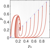
(a) Phase Portrait

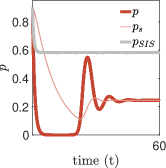
(b) Undershoot and overshoot

Figure 3: The EE as a stable focus. (a) Phase portrait of the actSIS model for a homogeneous population of risk-averters. Grey arrows depict the vector fields. The initial conditions and end points of the simulations are plotted as circles and squares respectively. Starting from low initial values, $p$ exhibits a rapid increase followed by a decrease to the EE. Starting from high initial values, $p$ exhibits a rapid decrease to nearly zero before an increase to the equilibrium state. (b) For $p(0)=p_{s}(0)=0.9$, the transient state $p$ undershoots to near zero for a long time and then overshoots. The parameters are $\bar{\beta}=2.4,\mu_{A}=0.25,\nu_{A}=8$.

For homogeneous risk-averters, (4) undergoes a transcritical bifurcation, as in the SIS model, but with a reduced EE, as illustrated in Fig. 2(b). Further, the EE becomes a stable focus under certain conditions, resulting in large overshoot and/or undershoot in the transient dynamics, as illustrated in Fig. 3.

We devote the rest of this section to the detailed description and proof of these rich dynamics. For simplicity of exposition, we set $\delta=1,\tau_{s}=10$ throughout the rest of this paper.

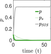
(a) IFE

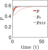
(b) EE

Figure 1: Bi-stability of risk-tolerators. The IFE and EE are both stable solutions for $\bar{\beta}>\bar{\beta}_{c}$ in the actSIS model for risk-tolerators. a) For $p(0)=0.1$, the solution (green) of actSIS (risk-tolerators) converges to the IFE, whereas the solution (grey) of SIS (risk-ignorers) converges to the EE. b) For $p(0)=0.4$, the solution (red) of actSIS and the solution (grey) of SIS converge to the EE. Parameters for all simulations are $\bar{\beta}=2.4,\mu_{T}=0.35,\nu_{T}=8.$ For these parameters, $\bar{\beta}_{c}=1.87<\bar{\beta}$.

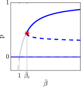
(a) Risk-tolerators

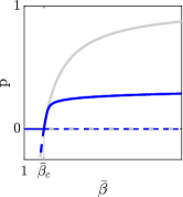
(b) Risk-averters

Figure 2: Bifurcation diagrams of the actSIS model. a) For homogeneous risk-tolerators, the actSIS model undergoes a saddle-node bifurcation at bifurcation point $\bar{\beta}_{c}>1$. b) For homogeneous risk-averters, the actSIS model undergoes a transcritical bifurcation at $\bar{\beta}=1$ as in the SIS model. The EE for the actSIS models are upper-bounded by that of the SIS model in both cases. The bifurcation diagrams of the actSIS models are drawn in blue and the SIS in grey. Solid curves denote stable solutions and dashed curves denote unstable solutions. Parameters for these plots are $\mu_{T}=0.35,\nu_{T}=8,\mu_{A}=0.25,\nu_{A}=8.$ The bifurcation diagrams: Fig.1 and Fig. 4 (a), are produced with the MATLAB package matcont (Dhooge et al. (2003)).

Theorem 3.1 (Steady-state behavior of the actSIS model with homogeneous risk-tolerators)

Consider the actSIS dynamics for a homogeneous population of risk-tolerators given by (4) with $r(t)=0$ and $\alpha(\cdot)=\phi^{T}(\cdot)$. Then the following hold:

1. There are two types of equilibrium solutions:

   1. IFE: $p=p_{s}=0$. It is always stable;

   2. EE: $p=p_{s}=p^{*}$ satisfying $\phi^{T}(p^{*})(1-p^{*})=\frac{\delta}{\bar{\beta}}$. There are zero, one, or two such solutions. A solution is stable if $\Phi^{T\prime}(p^{*})\cdot(1-p^{*})^{2}<\frac{\delta}{\bar{\beta}}$.

2. The system undergoes a saddle node bifurcation at the bifurcation point $(\bar{\beta}_{c},p^{*})$ with stable upper branch (stable EE) and unstable lower branch (unstable EE). The epidemic threshold $\bar{\beta}_{c}/\delta$ is always larger than that of the SIS model, i.e., $\bar{\beta}_{c}/\delta>1$.

3. For $\bar{\beta}>\bar{\beta}_{c}$ the system exhibits bistability of the IFE and the EE. For $\bar{\beta}\leq\bar{\beta}_{c}$ the IFE is the only stable equilibrium.

4. As $\bar{\beta}_{c}<\bar{\beta}\rightarrow\infty$, $p^{*}\rightarrow 1-\delta/\bar{\beta}$, the EE of SIS.

Proof.

1. The equilibrium solutions are straightforward to compute. For stability, we compute the Jacobian as

   $$J^{T}=\begin{bmatrix}\bar{\beta}\phi^{T}(p_{s})(1-2p)-\delta&\bar{\beta}(1-p)p{\phi^{T}}^{\prime}(p_{s})\\ \frac{1}{\tau_{s}}&-\frac{1}{\tau_{s}}\end{bmatrix}.$$ (7)

   For the IFE, (7) reduces to

   $$\left.J^{T}\right|_{\text{IFE}}=\begin{bmatrix}-\delta&0\\ \frac{1}{\tau_{s}}&-\frac{1}{\tau_{s}}\end{bmatrix},$$ (8)

   implying that the IFE is always stable. For the EE,

   $$\left.J^{T}\right|_{\text{EE}}=\begin{bmatrix}-\delta\frac{p^{*}}{1-p^{*}}&\bar{\beta}(1-p^{*})p^{*}{\phi^{T}}^{\prime}(p^{*})\\ \frac{1}{\tau_{s}}&-\frac{1}{\tau_{s}}\end{bmatrix}.$$ (9)

   Stability requires the equilibrium solution to satisfy $\frac{\delta}{1-p^{*}}-\bar{\beta}(1-p^{*})\phi^{T\prime}(p^{*})>0$. Since $p^{*}\in(0,1)$ , it is equivalent to requiring that $\phi^{T\prime}(p^{*})\cdot(1-p^{*})^{2}<\frac{\delta}{\bar{\beta}}$.

2. We start by computing the critical value $\bar{\beta}_{c}$. Since $\phi^{T}(\cdot)$ is a monotonically increasing function taking values between 0 and 1, $g(p):=\phi^{T}(p)(1-p)$ takes value between 0 and 1 and it first increases from 0 (since $g(0)=0$) and then decreases to 0 ($g(1)=0$). Depending on parameter values ($\mu_{T},\nu_{T},\bar{\beta},\delta$), the EE has either zero, one or two solutions. Let $h(p):=\phi^{T\prime}(p)\cdot(1-p)^{2}$. It first increases and then decreases for $p\in[0,1]$. Denoting $\hat{p}:=\mathop{\mathrm{argmax}}\limits_{p}g(p)$, one can check that $h(p)$ intersects with $g(p)$ at three points: $0,\hat{p}$ and $1$. This implies that when the EE has two solutions (when $\delta/\beta<g(\hat{p})$), the smaller solution is unstable and the larger one is stable. $\bar{\beta}_{c}$ can be solved analytically by solving $\bar{\beta}_{c}=\delta/g(\hat{p})$.

   To prove the existence of a saddle-node bifurcation, we use the classification of equilibria for a two-dimensional system presented in Section 4.2.5 in Izhikevich (2007). Specifically, we show that one of the eigenvalues of the Jacobian at $(\bar{\beta}_{c},p^{*})$ becomes zero. Using equations $\bar{\beta}_{c}=\delta/g(\hat{p})$ and $g^{\prime}(\hat{p})=0$, one can easily verify the determinant of the Jacobian at $(\bar{\beta}_{c},p^{*})$ equals zero thus the existence of a saddle node bifurcation.

   Since $g(\hat{p})\in(0,1)$, we have $\bar{\beta}_{c}/\delta$ is always larger than the epidemic threshold in the SIS model.

3. This follows directly from (i) and (ii).

4. Comparing the equations satisfied by the EE solutions for the SIS and the homogeneous actSIS (risk-tolerators) model, we observe that $\phi^{T}(p^{*})$ and $p^{*}$ increase with $\bar{\beta}$. As $\phi^{T}(p^{*})$ approaches $1$, $p^{*}$ approaches $1-\delta/\bar{\beta}$.

∎

Theorem 3.2 (Steady-state behavior of the actSIS model with homogeneous risk-averters)

Consider the actSIS dynamics for a homogeneous population of risk-averters given by (4) with $r(t)=0$ and $\alpha(\cdot)=1-\phi^{A}(\cdot)$. Then the following hold:

1. There are two equilibrium solutions:

   1. IFE: $p_{s}=p=0$. It is stable if $\bar{\beta}<\delta$;

   2. EE: $p_{s}=p=p^{*}$ satisfying $(1-\Phi^{A}(p^{*}))(1-p^{*})=\delta/\bar{\beta}$. It is always stable if it exists, which is when $\bar{\beta}>\delta$.

2. The EE is a stable focus if $b>(a-c)^{2}/(4ac)$, where $a=\frac{\delta p^{*}}{1-p^{*}},b=\frac{1-p^{*}}{1-\phi^{A}(p^{*})}\phi^{A\prime}(p^{*}),c=\frac{1}{\tau_{s}}$.

3. The EE is always upper bounded by $1-\delta/\bar{\beta}$, the SIS EE.

Proof.

1. Since $1-\Phi^{A}(\cdot)$ is monotone decreasing, there exists at most one EE solution when $\delta/\bar{\beta}<1$. The Jacobian of (4) is

   $$J=\begin{bmatrix}\bar{\beta}(1-\Phi^{A}(p_{s}))(1-2p)-\delta&-\bar{\beta}(1-p)p\phi^{A\prime}(p_{s})\\ \frac{1}{\tau_{s}}&-\frac{1}{\tau_{s}}\end{bmatrix},$$ (10)

   which simplifies to

   $$\left.J\right|_{\text{IFE}}=\begin{bmatrix}\bar{\beta}-\delta&0\\ \frac{1}{\tau_{s}}&-\frac{1}{\tau_{s}}\end{bmatrix},$$ (11)

   for the IFE, and

   $$\left.J\right|_{\text{EE}}=\begin{bmatrix}-\frac{\delta p^{*}}{1-p^{*}}&-\bar{\beta}(1-p^{*})p^{*}\phi^{A\prime}(p^{*})\\ \frac{1}{\tau_{s}}&-\frac{1}{\tau_{s}}\end{bmatrix}$$ (12)

   for the EE. Therefore, the IFE is stable when $\bar{\beta}<\delta$. For the EE, stability requires $\frac{\delta p^{*}}{1-p^{*}}+\bar{\beta}(1-p^{*})p^{*}\Phi^{A\prime}(p^{*})>0$. Since ${\Phi^{A}}^{\prime}(p^{*})$ is always non-negative, the stability conditions always holds when such a solution exists.

2. We prove when EE is a stable focus, by proving when (12) has a pair of complex-conjugate eigenvalues with negative real part. We use the classification of equilibria for a two-dimensional system according to the trace and determinant of the Jacobian (Izhikevich (2007)). Denoting $A:=\left.J\right|_{\text{EE}}$ and using the definitions of $a,b$ and $c$, we have $\operatorname{Tr}(A)=-(a+c)$ and $\det(A)=ac(1+b)$. Therefore the condition $b>\frac{(a-c)^{2}}{4ac}$, guarantees that $\operatorname{Tr}(A)^{2}-4\det(A)<0$, and together with $\operatorname{Tr}(A)<0$, that the EE is a stable focus.

3. As $\bar{\beta}$ increases, the right hand side of $(1-\Phi^{A}(p^{*}))(1-p^{*})=\delta/\bar{\beta}$ decreases. As a result, $p^{*}$ increases with $\bar{\beta}$. On the other hand, $1-\phi^{A}(p^{*})$ decreases away from $1$ thus the EE are always bounded above by $1-\delta/\bar{\beta}$.

∎

4 Heterogeneous Population

We introduce the heterogeneous network actSIS model. The transmission rates, recovery rates and feedback responses can all be distinct. However, we restrict to the following set up as a first step in exploring the role of heterogeneity. Let the population comprise two homogeneous sub-populations, risk-tolerators and risk-averters, which differ only in their feedback responses to the infection. We assume the disease transmission occurs across sub-populations but not within. For the generalization of the network SIS model (3) to the network actSIS model, this translates as $n=2$, $\bar{\beta}_{i}=\bar{\beta}$, $\delta_{i}=\delta$, $\beta_{ii}=0$, $\alpha(\cdot)=\alpha^{1}(\cdot)$ for all risk-tolerators and $\alpha(\cdot)=\alpha^{2}(\cdot)$ for all risk-averters. Let $p_{1}(t)$ ($p_{2}(t)$) denote the fraction of risk-tolerators (risk-averters) that are infected at time $t$. Let $\beta_{12}=\bar{\beta}\alpha^{1}(p_{s_{2}})=\bar{\beta}\phi^{T}\left(p_{s_{2}}\right)$ be the effective infection rate from risk-averters to risk-tolerators, and $\beta_{21}=\bar{\beta}\alpha^{2}(p_{s_{1}})=\bar{\beta}\left(1-\phi^{A}\left(p_{s_{1}}\right)\right)$ from risk-tolerators to risk-averters. The heterogeneous network actSIS model in the case of these two subpopulations is

$$\dot{p}_{1}=\left(1-p_{1}\right)\beta_{12}\cdot p_{2}-\delta p_{1},$$ (13)

$$\dot{p}_{2}=\left(1-p_{2}\right)\beta_{21}\cdot p_{1}-\delta p_{2},$$

$$\tau_{s}\dot{p}_{s_{1}}=-p_{s_{1}}+p_{1},$$

$$\tau_{s}\dot{p}_{s_{2}}=-p_{s_{2}}+p_{2}.$$

The equilibrium solutions satisfy $p_{1}^{*}=p_{s_{1}}^{*},p_{2}^{*}=p_{s_{2}}^{*}$ and

$$\frac{p_{1}^{*}}{1-p_{1}^{*}}\cdot\frac{1}{\alpha^{1}\left(p_{2}^{*}\right)p_{2}^{*}}=\frac{p_{2}^{*}}{1-p_{2}^{*}}\cdot\frac{1}{\alpha^{1}\left(p_{2}^{*}\right)p_{1}^{*}}=\frac{\delta}{\bar{\beta}}.$$ (14)

As shown in Fig. 4(a), there are model parameters for which system (13) undergoes a Hopf bifurcation with a stable limit cycle. As $\bar{\beta}$ increases from zero, system (13) undergoes a saddle-node bifurcation from a single stable IFE to bistability of the EE and the IFE. As $\bar{\beta}$ increases further across the Hopf bifurcation point $\bar{\beta}^{*}$, the system exhibits a stable limit cycle about the EE. For completeness, we present the following theorem (Theorem 3.4.2 in Guckenheimer and Holmes (1983)), which we use to prove the existence of stable limit cycles for (13).

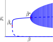
(a) Hopf bifurcation of system (13)

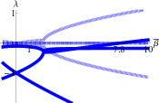
(b) Verification of (H2)

Figure 4: Hopf bifurcation. (a) Bifurcation diagram for $p_{1}$ with bifurcation parameter $\bar{\beta}$. For small positive values of $\bar{\beta}$, the IFE is the only stable solution. As $\bar{\beta}$ increases a saddle-node bifurcation leads to bistability of the IFE and EE. As $\bar{\beta}$ continues to increase there is a Hopf bifurcation (red dot) and stable oscillations about the EE. The blue solid curves depict stable solutions, while dashed curves depict unstable solutions. (b) The real and imaginary parts of the eigenvalues of the Jacobian $D_{p}\boldsymbol{f}$ at $(\boldsymbol{p}^{\mathbf{*}},\bar{\beta}^{*})$ are plotted in solid and dashed lines. At around $\bar{\beta}^{*}=7.8$, a pair of complex eigenvalues crosses the real line ($x$-axis) with a nonzero derivative, verifying (H2). Parameters are $\delta=1,\tau_{s}=10,\mu_{T}=0.45,\nu_{T}=0.8,\mu_{A}=0.45,\nu_{A}=20.$

Theorem 4.1 (Guckenheimer and Holmes)

Suppose that the heterogeneous actSIS model (13) expressed as $\dot{\boldsymbol{p}}=\boldsymbol{f}(\boldsymbol{p},\bar{\beta})$, $\boldsymbol{p}=(p_{1},p_{2},p_{s_{1}},p_{s_{2}})$, $\bar{\beta}\in\mathbb{R}$, has an equilibrium at $\left(\boldsymbol{p}^{\mathbf{*}},\bar{\beta}^{*}\right)$ and the following properties are satisfied:

• ($\mathrm{H}1$)   The Jacobian $\left.D_{p}\boldsymbol{f}\right|_{\left(\boldsymbol{p}^{\mathbf{*}},\bar{\beta}^{*}\right)}$ has a simple pair of pure imaginary eigenvalues $\lambda\left(\bar{\beta}^{*}\right)$ and $\overline{\lambda\left(\bar{\beta}^{*}\right)}$ and no other eigenvalues with zero real parts,

• $\left.(\mathrm{H}2)\;\frac{d}{d\bar{\beta}}(\operatorname{Re}\lambda(\bar{\beta}))\right|_{\left(\bar{\beta}=\bar{\beta}^{*}\right)}\neq 0$.

Then the dynamics undergo a Hopf bifurcation at $\left(\boldsymbol{p}^{\mathbf{*}},\bar{\beta}^{*}\right)$ resulting in periodic solutions. The stability of the periodic solutions is given by the sign of the first Lyapunov coefficient of the dynamics $\left.\ell_{1}\right|_{\left(\boldsymbol{p}^{\mathbf{*}},\bar{\beta}^{*}\right)}.$ If $\ell_{1}<0,$ then these solutions are stable limit cycles and the Hopf bifurcation is supercritical, while if $\ell_{1}>0,$ the periodic solutions are repelling.

We show in Proposition 4.2 conditions on the model parameters that guarantee that the non-hyperbolicity condition (H1) is satisfied for the heterogeneous actSIS model (13). We verify numerically that condition (H2) is satisfied and $\ell_{1}<0$.

Proposition 4.2

Denote $m=(1-p_{1}^{*})(1-p_{2}^{*})$, $q=p_{1}^{*}\beta_{21}^{*}/p_{2}^{*}$, $s=p_{2}^{*}\beta_{12}^{*}/p_{1}^{*}$, $v=p_{1}^{*}\beta_{21}^{\prime*}/p_{2}^{*}$, $w=p_{2}^{*}\beta_{12}^{\prime*}/p_{1}^{*}$, $\beta_{12}^{*}=\bar{\beta}\alpha^{1}\left(p_{2}^{*}\right),$ $\beta_{21}^{*}=\bar{\beta}\alpha^{2}\left(p_{1}^{*}\right))$. Then, for system (13), the non-hyperbolicity condition (H1) in Theorem 4.1 is satisfied if

$$c>0,\quad a\neq 0,$$

where

$$a :=s+q+\frac{2}{\tau_{s}},$$

$$ac :=\frac{2}{\tau_{s}}(1-m)sq+\frac{1}{\tau_{s}^{2}}(s+q)-m(v\beta_{12}^{*}+w\beta_{21}^{*}).$$

Proof.

For a four-dimensional system to satisfy (H1)
the eigenvalues of the Jacobian $\left.D_{p}\boldsymbol{f}\right|_{\left(\boldsymbol{p}^{\mathbf{*}},\bar{\beta}^{*}\right)}$ must satisfy

$$\left(\lambda^{2}+c\right)\left(\lambda^{2}+a\lambda+b\right)=0,$$ (15)

for some $a\neq 0$,$b\in\mathbb{R}$,and $c>0$. We compute the Jacobian
$\displaystyle\left.D_{p}\boldsymbol{f}\right|_{\left(\boldsymbol{p}^{\mathbf{*}},\bar{\beta}^{*}\right)}=\begin{bmatrix}-\beta_{12}^{*}p_{2}^{*}-\delta&(1-p_{1}^{*})\beta_{12}^{*}&0&(1-p_{1}^{*})p_{2}^{*}\beta_{12}^{\prime*}\\ (1-p_{2}^{*})\beta_{21}^{*}&-\beta_{21}^{*}p_{1}^{*}-\delta&(1-p_{2}^{*})p_{1}^{*}\beta_{21}^{\prime*}&0\\ \frac{1}{\tau_{s}}&0&-\frac{1}{\tau_{s}}&0\\ 0&\frac{1}{\tau_{s}}&0&-\frac{1}{\tau_{s}}\\ \end{bmatrix}$ which has eigenvalues that satisfy

$$\left(\frac{1}{\tau_{s}}+\lambda\right)^{2}\left(s+\lambda\right)\left(q+\lambda\right)-m\left(\frac{1}{\tau_{s}}+\lambda\right)^{2}sq$$ (16)

$$-m\left(\frac{1}{\tau_{s}}+\lambda\right)v\beta_{12}^{*}-m\left(\frac{1}{\tau_{s}}+\lambda\right)w\beta_{21}^{*}-mvw =0.$$

Matching coefficients of (15) and (16), we derive the expressions for $a$, $b$, and $c$, in terms of the model parameters ($\bar{\beta},\mu_{T},\gamma_{T},\mu_{A},\gamma_{A}$) for (13) to satisfy the first part of (H1). We have $\lambda\left(\bar{\beta}^{*}\right)=\sqrt{c}\mathrm{i}$, a pure imaginary eigenvalue. $a\neq 0$ guarantees there are no other eigenvalues with zero real part. ∎

A proof of conditions guaranteeing (H2) of Theorem 4.1 is the subject of ongoing work. Fig 4(b) shows numerically that (H2) is satisfied for the parameters selected. We also checked that $\ell_{1}<0$. An illustration of the sustained oscillations corresponding to the stable limit cycle of (13) is depicted in Fig 5.

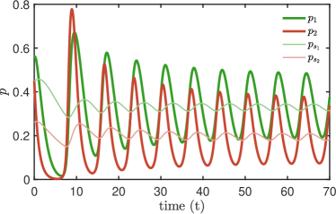
(a) Sustained oscillations

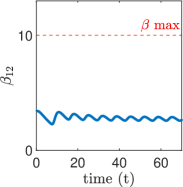
(b) $\beta_{12}$ evolution

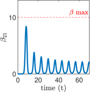
(c) $\beta_{21}$ evolution

Figure 5: Stable limit cycles of the heterogeneous actSIS model. a) When $\bar{\beta}>\bar{\beta}^{*}$, system (13) exhibits stable oscillations. States $p_{1}$ and $p_{2}$ initially decrease quickly due to different mechanisms: $p_{1}$ decreases because $p_{s_{2}}(0)<\mu_{T}$, which drives $\beta_{12}$ down and $p_{2}$ decreases because $p_{s_{1}}(0)>\mu_{A}$, which drives $\beta_{21}$ down. The low $p_{1}$ leads to a decrease in $p_{s_{1}}$, which in turn drives up $\beta_{21}$, thus increasing $p_{2}$. The increase in $p_{2}$ leads to an increase in $p_{s_{2}}$, which in turn drives up $p_{1}$. The process repeats resulting in sustained oscillations. b-c): The time evolution of the effective infection rates. Parameters used for the simulation: $\bar{\beta}=8.8$, $\mu_{T}=0.45,\nu_{T}=0.8,\mu_{A}=0.3,\nu_{A}=20$. Initial conditions: $p_{1}(0)=0.55,p_{2}(0)=0.45,p_{s_{1}}(0)=0.45,p_{s_{2}}(0)=0.66.$

5 Final remarks

The actSIS model incorporates two novel mechanisms as compared with the SIS model: a feedback mechanism for the effective infection rates, and a time scale separation between the state of the system and the state used in the feedback law. The qualitative differences we have shown for the actSIS model are due to both of the mechanisms. We have observed sustained oscillations even when some of the individuals are risk-ignorers and under relaxed assumptions on interconnections. We will examine the broader set of possibilities in future work and consider applications in other biological and socio-ecological processes.

References

- Anderson and May (1992) Anderson, R.M. and May, R.M. (1992). Infectious diseases of humans: dynamics and control. Oxford University Press.
- Antweiler (2018) Antweiler, W. (2018). A sigmoid-logit probability function for the (0,1) domain. URL http://wernerantweiler.ca/blog.php?item=2018-11-03.
- Baker (2020) Baker, R. (2020). Reactive social distancing in a SIR model of epidemics such as COVID-19. arXiv:2003.08285v1.
- Camacho et al. (2011) Camacho, A., Ballesteros, S., Graham, A.L., Carrat, F., Ratmann, O., and Cazelles, B. (2011). Explaining rapid reinfections in multiple-wave influenza outbreaks: Tristan da cunha 1971 epidemic as a case study. Proceedings of the Royal Society B: Biological Sciences, 278(1725), 3635–3643.
- Demiris et al. (2014) Demiris, N., Kypraios, T., and Smith, L.V. (2014). On the epidemic of financial crises. Journal of the Royal Statistical Society. Series A (Statistics in Society), 697–723.
- Dhooge et al. (2003) Dhooge, A., Govaerts, W., and Kuznetsov, Y.A. (2003). MATCONT: a MATLAB package for numerical bifurcation analysis of ODEs. ACM Transactions on Mathematical Software (TOMS), 29(2), 141–164.
- Diekmann et al. (1990) Diekmann, O., Heesterbeek, J.A.P., and Metz, J.A. (1990). On the definition and the computation of the basic reproduction ratio R0 in models for infectious diseases in heterogeneous populations. J. of Mathematical Biology, 28(4), 365–382.
- Dushoff et al. (2004) Dushoff, J., Plotkin, J.B., Levin, S.A., and Earn, D.J. (2004). Dynamical resonance can account for seasonality of influenza epidemics. Proc. National Academy of Sciences, 101(48), 16915–16916.
- Fall et al. (2007) Fall, A., Iggidr, A., Sallet, G., and Tewa, J.J. (2007). Epidemiological models and lyapunov functions. Mathematical Modelling of Natural Phenomena, 2(1), 62–83.
- Franco (2020) Franco, E. (2020). A feedback SIR (fSIR) model highlights advantages and limitations of infection-based social distancing. sociarXiv:2004.13216v1s.
- Funk et al. (2009) Funk, S., Gilad, E., Watkins, C., and Jansen, V.A. (2009). The spread of awareness and its impact on epidemic outbreaks. Proc. National Academy of Sciences, 106(16), 6872–6877.
- Guckenheimer and Holmes (1983) Guckenheimer, J. and Holmes, P. (1983). Nonlinear Oscillations, Dynamical Systems, and Bifurcations of Vector Fields. Springer-Verlag.
- Hartmann et al. (2008) Hartmann, W.R., Manchanda, P., Nair, H., Bothner, M., Dodds, P., Godes, D., Hosanagar, K., and Tucker, C. (2008). Modeling social interactions: Identification, empirical methods and policy implications. Marketing Letters, 19(3-4), 287–304.
- Hethcote and Yorke (1984) Hethcote, H.W. and Yorke, J.A. (1984). Lecture Notes in Biomathematics. Springer.
- Izhikevich (2007) Izhikevich, E.M. (2007). Dynamical Systems in Neuroscience. MIT press.
- Jin et al. (2013) Jin, F., Dougherty, E., Saraf, P., Cao, Y., and Ramakrishnan, N. (2013). Epidemiological modeling of news and rumors on twitter. In Proceedings of the 7th Workshop on Social Network Mining and Analysis, 1–9.
- Kermack and McKendrick (1927) Kermack, W.O. and McKendrick, A.G. (1927). A contribution to the mathematical theory of epidemics. Proceedings of the Royal Society of London. Series A, 115(772), 700–721.
- Lajmanovich and Yorke (1976) Lajmanovich, A. and Yorke, J.A. (1976). A deterministic model for gonorrhea in a nonhomogeneous population. Mathematical Biosciences, 28(3-4), 221–236.
- Lin et al. (1999) Lin, J., Andreasen, V., and Levin, S.A. (1999). Dynamics of influenza A drift: the linear three-strain model. Mathematical Biosciences, 162, 33–51.
- Mei et al. (2017) Mei, W., Mohagheghi, S., Zampieri, S., and Bullo, F. (2017). On the dynamics of deterministic epidemic propagation over networks. Annual Reviews in Control, 44, 116–128.
- Mishchenko (2014) Mishchenko, Y. (2014). Oscillations in rational economies. PloS One, 9(2), e87820.
- Muench (1934) Muench, H. (1934). Derivation of rates from summation data by the catalytic curve. Journal of the American Statistical Association, 29(185), 25–38.
- Nowzari et al. (2016) Nowzari, C., Preciado, V.M., and Pappas, G.J. (2016). Analysis and control of epidemics: A survey of spreading processes on complex networks. IEEE Control Syst. Mag., 36(1), 26–46.
- Pagliara and Leonard (2020) Pagliara, R. and Leonard, N.E. (2020). Adaptive susceptibility and heterogeneity in contagion models on networks. IEEE Transactions on Automatic Control. 10.1109/TAC.2020.2985300.
- Pais et al. (2012) Pais, D., Caicedo-Nunez, C.H., and Leonard, N.E. (2012). Hopf bifurcations and limit cycles in evolutionary network dynamics. SIAM Journal on Applied Dynamical Systems, 11(4), 1754–1784.
- Rands (2010) Rands, S.A. (2010). Group movement ’initiation’ and state-dependent decision-making. Behavioural Processes, 84(3), 668–670.
- Sahneh et al. (2013) Sahneh, F.D., Scoglio, C., and Van Mieghem, P. (2013). Generalized epidemic mean-field model for spreading processes over multilayer complex networks. IEEE/ACM Transactions on Networking, 21(5), 1609–1620.
- Sepulchre et al. (2019) Sepulchre, R., Drion, G., and Franci, A. (2019). Control across scales by positive and negative feedback. Annual Review of Control, Robotics, and Autonomous Systems, 2, 89–113.
- Smaldino et al. (2018) Smaldino, P.E., Aplin, L.M., and Farine, D.R. (2018). Sigmoidal acquisition curves are good indicators of conformist transmission. Scientific Reports, 8(1), 1–10.
- Xu et al. (2020) Xu, B., Cai, J., He, D., Chowell, G., and Xu, B. (2020). Mechanistic modelling of multiple waves in an influenza epidemic or pandemic. Journal of Theoretical Biology, 486, 110070.
- Zhao et al. (2014) Zhao, L., Wang, J., Huang, R., Cui, H., Qiu, X., and Wang, X. (2014). Sentiment contagion in complex networks. Physica A: Statistical Mechanics and its Applications, 394, 17–23.