Dualities for three-dimensional $\mathcal{N}=2$ $SU(N_{c})$ chiral adjoint SQCD

Abstract

We study dualities for 3d $\mathcal{N}=2$ $SU(N_{c})$ SQCD at Chern–Simons level $k$ in presence of an adjoint with polynomial superpotential. The dualities are dubbed chiral because there is a different amount of fundamentals $N_{f}$ and antifundamentals $N_{a}$. We build a complete classification of such dualities in terms of $|N_{f}-N_{a}|$ and $k$. The classification is obtained by studying the flow from the non-chiral case, and we corroborate our proposals by matching the three-sphere partition functions. Finally, we revisit the case of $SU(N_{c})$ SQCD without the adjoint, comparing our results with previous literature.

1 Introduction

The rich web of 3d $\mathcal{N}=2$ infrared dualities represents an active field of research both because of its similarities with less or non-supersymmetric cases, and because of its connection with exact results in mathematical physics through localization. This latter aspect led to a systematic study of many physical dualities, once the formal structure of the three-sphere partition function of $\mathcal{N}=2$ models was successfully computed via localization in Kapustin:2009kz ; Jafferis:2010un ; Hama:2010av ; Hama:2011ea . Indeed it was soon realized Willett:2011gp ; Benini:2011mf that the identities among the partition functions of the dualities known at the time, namely Aharony Aharony:1997gp and Giveon–Kutasov Giveon:2008zn dualities, already appeared in the mathematical literature as integral identities among hyperbolic hypergeometric gamma functions VanDeBult . This result was interesting also because many other integral identities were available in the mathematical literature, suggesting the existence of yet-to-be-discovered dualities. Indeed for $U(N_{c})$ SQCD the systematic analysis of Benini:2011mf provided a classification scheme for chiral dualities. This name originates from the fact that such dualities feature in general a different number of fundamental and antifundamental matter fields.

In this paper we study chiral dualities for 3d $\mathcal{N}=2$ SQCD with $SU(N_{c})$ gauge group, Chern–Simons (CS) interactions, and adjoint matter, extending the analysis of Aharony:2014uya ; Hwang:2015wna ; Nii:2019qdx ; Nii:2020xgd . For consistency with the classification of Benini:2011mf , we divide the dualities into two main classes denoted $[p,q]$ and $[p,q]^{*}$ (that we will review in section 2). In this classification it is possible to recover non-chiral dualities as well: Aharony duality corresponds to the $[0,0]$ case, and Giveon–Kutasov duality corresponds to the $[p,p]$ case. (Furthermore the $[0,0]$ and the $[p,0]$ cases require further singlets and interactions in the dual phase, with respect to the other dualities in the $[p,q]$ family.)

Two generalizations of the results of Benini:2011mf have been discussed in the literature.

• In Aharony:2014uya chiral dualities for $SU(N_{c})$ SQCD are tackled. The authors identify two classes of dualities that are reminiscent of the $[p,q]$ and $[p,q]^{*}$ classes of Benini:2011mf . Actually the relation between Aharony:2014uya and Benini:2011mf is more involved.

  Indeed by applying the standard procedure of gauging the topological symmetry of the $U(N_{c})$ case of Benini:2011mf one does not recover the $SU(N_{c})$ case of Aharony:2014uya . This is due to the presence of CS interactions: the application of local mirror symmetry is necessary to obtain the expected duality. This problem is reminiscent of the one discussed in Aharony:2013dha to connect Giveon–Kutasov duality for $U(N_{c})_{k}$ to the one for non-chiral $SU(N_{c})_{k}$ SQCD obtained from circle reduction of 4d Seiberg duality (in addition to a real mass flow).

• Another generalization of Benini:2011mf has been proposed in Hwang:2015wna , which studies dualities for $U(N_{c})$ chiral SQCD with adjoint matter. In this case the authors discuss the extension of the $[p,q]^{*}$ case, as well as the $[p,0]$ one, but neglect the general $[p,q]$ case. More recently, some discussion on dualities for $SU(N_{c})$ chiral SQCD with adjoint matter appeared in Nii:2019qdx . The author focuses on a specific $[p,q]^{*}$ case with vanishing CS level.

Motivated by these results, in this paper we provide a complete classification of 3d $\mathcal{N}=2$ infrared dualities for $SU(N_{c})$ chiral adjoint SQCD. In order to obtain such a classification we first reconsider the case of $SU(N_{c})$ chiral SQCD (section 3), obtaining a classification that slightly differs from the one of Aharony:2014uya , and then discuss the generalization of Benini:2011mf to the case of $U(N_{c})$ with adjoint matter (section 4). Finally we study the case of $SU(N_{c})$ with adjoint matter and provide a classification of chiral dualities (section 5). As a check of our proposals we match the three-sphere partition functions. Our results are summarized in tables 1 and 2. In section 6 we briefly present our conclusions.

Several appendices complement our analysis. In appendix A we show how to distinguish the $SU(N_{c})_{k_{1}}$ from the $U(1)_{k_{2}}$ CS contribution in the localized three-sphere partition function of $U(N_{c})_{k_{1},k_{1}+N_{c}k_{2}}$. In appendix B we write down the real mass flow (starting from the $SU(N_{c})$ version of Giveon–Kutasov duality appearing in Aharony:2013dha ) producing the dualities of (Aharony:2014uya, ) at the level of the partition function. In appendix C we write down the real mass flow (again starting from the $SU(N_{c})_{k}$ duality of Aharony:2013dha ) producing the dualities of section 3, i.e. a reformulation of the chiral dualities of Aharony:2014uya . The interrelation between the sections and appendices of this paper and previous literature is presented in figures 1, 2, and 3. Finally in appendix D we discuss the D3-D5-NS5 brane engineering of the dualities of Benini:2011mf .

2 Known dualities for $U(N_{c})$ and $SU(N_{c})$ chiral SQCD

The mathematical notation $[p,q]$, $[p,q]^{*}$ we mentioned in the introduction can be traded for a more physical one in terms of the effective CS level on the Coulomb branch of a $U(N_{c})_{k}$ gauge theory. Defining

$$k_{\pm}\equiv k\pm\frac{1}{2}(N_{f}-N_{a})\ ,$$ (1)

we have Benini:2011mf :

$$[p,q]_{a}\equiv[-k_{+},-k_{-}]_{a}\ , [p,q]_{b}\equiv[k_{+},k_{-}]_{b}\ ,$$ (2a)

$$[p,q]_{a}^{*}\equiv[-k_{+},k_{-}]_{a}^{*}\ , [p,q]_{b}^{*}\equiv[k_{+},-k_{-}]_{b}^{*}\ ,$$ (2b)

where $\pm k_{\pm}$ represents the effective CS level on the Coulomb branch for positive and negative values of the real scalar $\sigma$ in the vector multiplet. The “type” of the theory (i.e. the subscript $a$ or $b$) is then determined by requiring $p,q\geq 0$. (In practice, given $\{k,N_{f},N_{a}\}$ one computes $k_{\pm}$ via (1) and picks the case where both $p$ and $q$ are non-negative. This selects the type of the theory.) Notice that the dual of a type-$a$ theory (be it in the $[p,q]$ or $[p,q]^{*}$ class) is a type-$b$ theory Benini:2011mf . Moreover the cases $[p,0]$ and $[0,q]$ are obtained as limiting cases of $[p,q]$ in the obvious way.

With this notation in place, we are ready to collect the results that have been obtained in the literature so far. Chiral dualities for $U(N_{c})$ gauge theories were studied in Benini:2011mf . In the $[p,q]$ case we have a duality between:

• an electric model, consisting of $U(N_{c})_{k}$ SQCD with $N_{f}$ fundamentals $Q$, $N_{a}$ antifundamentals $\tilde{Q}$, $|N_{f}-N_{a}|<2k$, and vanishing superpotential, $W=0$;

• a magnetic model consisting of $U(\widetilde{N}_{c})_{-k}$ SQCD, where $\widetilde{N}_{c}\equiv\frac{1}{2}(N_{f}+N_{a})+k-N_{c}$, with $N_{f}$ fundamentals, $N_{a}$ antifundamentals, the meson $M=Q\tilde{Q}$, and $W=Mq\tilde{q}$.

Further, when $p$ and/or $q$ are vanishing these dualities are modified by the presence of extra singlets in the dual, magnetic, phase. These singlets are identified with the monopole operators of the electric phase. For example if both $p$ and $q$ are vanishing (the case of Aharony duality) we have:

• an electric model, consisting of $U(N_{c})$ SQCD with $N_{f}$ fundamentals $Q$, $N_{f}$ anti-fundamentals $\tilde{Q}$, and $W=0$;

• a magnetic model consisting of $U(\widetilde{N}_{c})$ SQCD, where $\widetilde{N}_{c}\equiv N_{f}-N_{c}$, with $N_{f}$ fundamentals, $N_{f}$ antifundamentals, the meson $M=Q\tilde{Q}$, two new singlets $T_{\pm}$ identified with the monopole and the anti-monopole of the electric phase, and $W=Mq\tilde{q}+T_{+}t_{-}+T_{-}t_{+}$, where $t_{\pm}$ are the monopole and the antimonopole of the dual phase.

If instead only $q=0$ we have:

• an electric model, consisting of $U(N_{c})_{(N_{f}-N_{a})/2}$ SQCD with $N_{f}$ fundamentals $Q$, $N_{a}<N_{f}$ antifundamentals $\tilde{Q}$, and $W=0$;

• a magnetic model consisting of $U(\widetilde{N}_{c})_{(N_{a}-N_{f})/2}$ SQCD, where $\widetilde{N}_{c}\equiv N_{f}-N_{c}$, with $N_{f}$ fundamentals, $N_{a}$ antifundamentals, the meson $M=Q\tilde{Q}$, a new singlet $T_{+}$, and $W=Mq\tilde{q}+T_{+}t_{-}$.

In the $[p,q]^{*}$ case we have a duality between:

• an electric model, consisting of $U(N_{c})_{k}$ SQCD with $N_{f}$ fundamentals $Q$, $N_{a}$ antifundamentals $\tilde{Q}$, $|N_{f}-N_{a}|>2k$, and $W=0$;

• a magnetic model consisting of $U(\widetilde{N}_{c})_{-k}$ SQCD, where $\widetilde{N}_{c}\equiv\max(N_{f},N_{a})-N_{c}$, with $N_{f}$ fundamentals, $N_{a}$ antifundamentals, the meson $M=Q\tilde{Q}$, and $W=Mq\tilde{q}$.

In the case of $SU(N_{c})$ a similar classification was obtained in Aharony:2014uya . The authors obtained the analog of the $[p,q]$ and $[p,q]^{*}$ classes. In the electric phase the theory corresponds to $SU(N_{c})_{k}$ SQCD with $N_{f}$ fundamentals $Q$, $N_{a}$ antifundamentals $\tilde{Q}$, and $W=0$. As in the classification of Benini:2011mf , the dual magnetic model depends instead on the relative value of $2k$ with respect to $\Delta F\equiv|N_{f}-N_{a}|$. If $\Delta F\leq 2k$ the dual model is $SU(\widetilde{N}_{c})_{-k}\times U(1)_{\widetilde{N}_{c}-k}$, where $\widetilde{N}_{c}\equiv\frac{1}{2}(N_{f}+N_{a})+k-N_{c}$, with $N_{f}$ fundamentals, $N_{a}$ antifundamentals, the meson $M=Q\tilde{Q}$, and $W=Mq\tilde{q}$. If $\Delta F>2k$ the dual model is $SU(\widetilde{N}_{c})_{-k}\times U(1)_{\tilde{N}_{c}-k}\times U(1)_{0}$, where $\widetilde{N}_{c}\equiv\max(N_{f},N_{a})-N_{c}$, with $N_{f}$ fundamentals, $N_{a}$ antifundamentals, the meson $M=Q\tilde{Q}$, and $W=Mq\tilde{q}$. There is also a mixed CS term, at level $1$, between the two $U(1)$ gauge groups.

Observe that the chiral class denoted $[p,0]$ in Benini:2011mf , corresponding to the case $\Delta F=2k$, was not distinguished from the case $\Delta F<2k$ in the analysis of Aharony:2014uya . More recently Nii:2020xgd claimed that actually these two cases are distinguished. In the following we will support this latter claim.

As observed in Aharony:2014uya the chiral dualities for $SU(N_{c})$ SQCD cannot be easily obtained from the ones for $U(N_{c})$ SQCD by gauging the topological $U(1)$ symmetry. This is because there are CS interactions that make this step nontrivial. Observe also that the $SU(N_{c})$ chiral dualities have been obtained starting from the non-chiral duality for $SU(N_{c})_{k}$ with matter. Nevertheless another possibility would be to start from the $SU(N_{c})$ version of Aharony duality (i.e. at zero CS level) obtained in Park:2013wta and then flow to the chiral $SU(N_{c})$ cases. This construction would be more similar to the one obtained in Benini:2011mf for the $U(N_{c})$ case. We are going to perform such a construction in the next section, and comment on the relation with Aharony:2014uya in appendix B.

We end this section by compactly presenting the known dualities for $U(N_{c})$ and $SU(N_{c})$ chiral SQCD in table 1. In section 3 we will rederive the chiral dualities for $SU(N_{c})$ SQCD, finding different dual descriptions than the ones presented in table 1. Their equivalence is then proven in appendix B. In table 2 we anticipate the results for $U(N_{c})$ and $SU(N_{c})$ chiral SQCD with one adjoint matter field, presented in section 4 and 5 respectively.

case	$|N_{f}-N_{a}|$ vs. $2k$	electric phase	magnetic phase	ref.
$[0,0]$	$0=0$	$U(N_{c})_{0}$ w/ $(N_{f},N_{f})$; $W=0$	$U(N_{f}-N_{c})_{0}$ w/ $(N_{f},N_{f}),M=Q\tilde{Q},T_{\pm}$; $W=Mq\tilde{q}+T_{+}t_{-}+T_{-}t_{+}$	Aharony:1997gp
$[p,0]$	$\Delta F=2k$	$U(N_{c})_{k}$ w/ $(N_{f},N_{a}),N_{a}<N_{f}$; $W=0$	$U(N_{f}-N_{c})_{-k}$ w/ $(N_{a},N_{f}),M=Q\tilde{Q},T_{+}$; $W=Mq\tilde{q}+T_{+}t_{-}$	Benini:2011mf
$[p,p]$	$0<2k$	$U(N_{c})_{k}$ w/ $(N_{f},N_{f})$; $W=0$	$U(N_{f}-N_{c}+|k|)_{-k}$ w/ $(N_{f},N_{f}),M=Q\tilde{Q}$; $W=Mq\tilde{q}$	Giveon:2008zn
$[p,q]$	$\Delta F<2k$	$U(N_{c})_{k}$ w/ $(N_{f},N_{a})$; $W=0$	$U(\tfrac{1}{2}(N_{f}+N_{a})+|k|-N_{c})_{-k}$ w/ $(N_{a},N_{f}),M=Q\tilde{Q}$; $W=Mq\tilde{q}$	Benini:2011mf
$[p,q]^{*}$	$\Delta F>2k$		$U(\max(N_{f},N_{a})-N_{c})_{-k}$ w/ $(N_{a},N_{f}),M=Q\tilde{Q}$; $W=Mq\tilde{q}$
$[0,0]$	$0=0$	$SU(N_{c})_{0}$ w/ $(N_{f},N_{f})$; $W=0$	$U(N_{f}-N_{c})_{0}$ w/ $(N_{f},N_{f}),(b,\tilde{b}),M=Q\tilde{Q},Y$; $W=\eqref{WARSW}$	Aharony:2013dha (Park:2013wta )
$[p,q]$	$\Delta F<2k$	$SU(N_{c})_{k}$ w/ $(N_{f},N_{a})$; $W=0$	$SU(\widetilde{N}_{c})_{-k}\times U(1)_{\widetilde{N}_{c}-k}$ $\widetilde{N}_{c}\equiv\tfrac{1}{2}(N_{f}+N_{a})+|k|-N_{c}$ w/ $(N_{a},N_{f}),M=Q\tilde{Q}$; $W=Mq\tilde{q}$	Aharony:2014uya
$[p,0]$	$\Delta F=2k$		$SU(\widetilde{N}_{c})_{-k}\times U(1)_{{\widetilde{N}_{c}}/{2}-k}$ $\widetilde{N}_{c}\equiv\tfrac{1}{2}(N_{f}+N_{a})+|k|-N_{c}$ w/ $(N_{a},N_{f}),M=Q\tilde{Q},T_{-}$; $W=$ (Nii:2020xgd, , Eq. (7.45))	Nii:2020xgd
$[p,q]^{*}$	$\Delta F>2k$		$SU(\widetilde{N}_{c})_{-k}\times(U(1)_{\widetilde{N}_{c}-k}\times U(1)_{0})_{1}$ $\widetilde{N}_{c}\equiv\max(N_{f},N_{a})-N_{c}$ w/ $(N_{a},N_{f}),M=Q\tilde{Q}$; $W=Mq\tilde{q}$	Aharony:2014uya

Table 1: Summary of chiral dualities for $U(N_{c})$ and $SU(N_{c})$ SQCD with $(N_{f},N_{a})\in(\mathbf{N}_{c},\overline{\mathbf{N}_{c}})$ matter fields. Here $U(N_{c})_{k}\equiv U(N_{c})_{k,k}=SU(N_{c})_{k}\times U(1)_{0}$ (neglecting global issues). The notation $(U(1)\times U(1))_{1}$ means there is a mixed CS term at level $1$ between the two gauge $U(1)$’s. (One of the two factors may be the abelian center of $U(\widetilde{N}_{c})$.) The dictionary between the non-negative integers $p,q$ and the effective CS level $k_{\pm}$ on the Coulomb branch is as in formulae (1)-(2).

case	$|N_{f}-N_{a}|$ vs. $2k$	electric phase	magnetic phase	ref.
$[0,0]_{\text{adj}}$	$0=0$	$U(N_{c})_{0}$ w/ $(N_{f},N_{f}),X$; $W=\operatorname{Tr}X^{n+1}$	$U(nN_{f}-N_{c})_{0}$ w/ $(N_{f},N_{f}),Y,M_{j}=QX^{j}\tilde{Q}$, $T_{j,+}=T_{+}X^{j},T_{j,-}=T_{-}X^{j}$, $j=0,\ldots,n-1$; $W=\eqref{wKP}$	Kim:2013cma
$[p,p]_{\text{adj}}$	$0<2k$	$U(N_{c})_{k}$ w/ $(N_{f},N_{f}),X$; $W=\operatorname{Tr}X^{n+1}$	$U(n(N_{f}+|k|)-N_{c})_{-k}$ w/ $(N_{f},N_{f}),Y,M_{j}=QX^{j}\tilde{Q}$, $j=0,\ldots,n-1$; $W=\eqref{Wniarchos}$	Niarchos:2008jb
$[p,q]_{\text{adj}}$	$\Delta F<2k$	$U(N_{c})_{k}$ w/ $(N_{f},N_{a}),X$; $W=\operatorname{Tr}X^{n+1}$	$U(n(\tfrac{1}{2}(N_{f}+N_{a})+|k|)-N_{c})_{-k}$ w/ $(N_{a},N_{f}),Y,M_{j}=QX^{j}\tilde{Q}$, $j=0,\ldots,n-1$; $W=\eqref{wd}$	here
$[p,0]_{\text{adj}}$	$\Delta F=2k$		$U(n(\tfrac{1}{2}(N_{f}+N_{a})+|k|)-N_{c})_{-k}$ w/ $(N_{a},N_{f}),Y,M_{j}=QX^{j}\tilde{Q}$, $T_{j,-}=T_{-}X^{j},\ j=0,\ldots,n-1$; $W=\eqref{wdd}$	Hwang:2015wna
$[p,q]^{*}_{\text{adj}}$	$\Delta F>2k$		$U(n\max(N_{f},N_{a})-N_{c})_{-k}$ w/ $(N_{a},N_{f}),Y,M_{j}=QX^{j}\tilde{Q}$, $j=0,\ldots,n-1$; $W=\eqref{Wddd}$
$[0,0]_{\text{adj}}$	$0=0$	$SU(N_{c})_{0}$ w/ $(N_{f},N_{f}),X$; $W=\operatorname{Tr}X^{n+1}$	$(U(nN_{f}-N_{c})_{0}\times U(1)_{0})_{1}$ w/ $(N_{f},N_{f}),Y,M_{j}=QX^{j}\tilde{Q}$, $(T_{j,+},T_{j,-})\in(+,-)$, $j=0,\ldots,n-1$; $W=\eqref{SU00adj}$	Park:2013wta
$[p,q]_{\text{adj}}$	$\Delta F<2k$	$SU(N_{c})_{k}$ w/ $(N_{f},N_{a}),X$; $W=\operatorname{Tr}X^{n+1}$	$(U(n(\tfrac{1}{2}(N_{f}+N_{a})+|k|)-N_{c})_{-k}\times U(1)_{-n})_{1}$ w/ $(N_{a},N_{f}),Y,M_{j}=QX^{j}\tilde{Q}$, $j=0,\ldots,n-1$; $W=\eqref{pqsuadj}$	here
$[p,0]_{\text{adj}}$	$\Delta F=2k$		$(U(nN_{f}-N_{c})_{-k}\times U(1)_{-n/2})_{1}$ w/ $(N_{a},N_{f}),Y,M_{j}=QX^{j}\tilde{Q}$, $T_{j,+}\in(+)$, $j=0,\ldots,n-1$; $W=\eqref{Wp0suadj}$
$[p,q]^{*}_{\text{adj}}$	$\Delta F>2k$		$(U(n\max(N_{f},N_{a})-N_{c})_{-k}\times U(1)_{0})_{1}$ w/ $(N_{a},N_{f}),Y,M_{j}=QX^{j}\tilde{Q}$, $j=0,\ldots,n-1$; $W=\eqref{wpqasdj*}$

Table 2: Summary of chiral dualities for $U(N_{c})$ and $SU(N_{c})$ adjoint SQCD with $(N_{f},N_{a})\in(\mathbf{N}_{c},\overline{\mathbf{N}_{c}})$ matter fields, and one field $X$ in the $\mathbf{Adj}$ of the electric gauge group. The dual adjoint field in the magnetic phase is $Y$. The notation is as in table 1.

3 Reformulating the dualities for $SU(N_{c})$ chiral SQCD

In this section we discuss the existence of families of 3d chiral dualities for $SU(N_{c})_{k}$ CS matter theories very similar to the ones derived in Aharony:2014uya . The main differences between the two families of dualities (i.e. ours and theirs) are the following:

• the case $\Delta F\equiv|N_{f}-N_{a}|<2k$ and $\Delta F=2k$ are treated separately in our description;

• there is a different amount of $U(1)$ gauge factors.

In appendix B we will then show that the dualities obtained here and the ones discussed in Aharony:2014uya ; Nii:2020xgd are related by some mirror transformations, similarly to what is expected in the non-chiral case Aharony:2013dha .

We derive the chiral dualities by flowing from the generalization of Aharony duality to $SU(N_{c})$ non-chiral SQCD with vanishing CS level. We perform a real mass flow on the electric side considering large vacuum expectation values (VEVs) for some of the scalars in the background vector multiplets associated to the global symmetries. This procedure leads to a chiral $SU(N_{c})$ model. Then we match this limit on the magnetic side, by considering also large VEVs for the scalars in the vector multiplet of the gauge symmetry.

On the electric side we have $SU(N_{c})_{0}$ SQCD with global $SU(N_{f})_{L}\times SU(N_{f})_{R}\times U(1)_{B}\times U(1)_{A}\times U(1)_{R}$ symmetry and vanishing superpotential. The charges are as follows:

$$\begin{array}[]{c|cccccc}&SU(N_{c})&SU(N_{f})_{L}&SU(N_{f})_{R}&U(1)_{B}&U(1)_{A}&U(1)_{R}\\ \hline\cr Q&\mathbf{N}_{c}&\mathbf{N}_{f}&\mathbf{1}&1&1&\Delta\\ \tilde{Q}&\overline{\mathbf{N}_{c}}&\mathbf{1}&\overline{\mathbf{N}_{f}}&-1&1&\Delta\\ \end{array}$$ (3)

The dual model is a $U(\widetilde{N}_{c})_{0}\times U(1)_{0}$ gauge theory, $\widetilde{N}_{c}\equiv N_{f}-N_{c}$, with a mixed CS term between the center $U(1)\subset U(\widetilde{N}_{c})$ and the other $U(1)$ gauge factor. The matter content is summarized in the following table:

$$\begin{array}[]{c|cccccc}&U(\widetilde{N}_{c})\times U(1)&SU(N_{f})_{L}&SU(N_{f})_{R}&U(1)_{B}&U(1)_{A}&U(1)_{R}\\ \hline\cr\rule{0.0pt}{15.0pt}q&\widetilde{\mathbf{N}}_{c,0}&\overline{\mathbf{N}_{f}}&\mathbf{1}&0&-1&1-\Delta\\ \tilde{q}&\overline{\widetilde{\mathbf{N}}_{c}}_{,0}&\mathbf{1}&\mathbf{N}_{f}&0&-1&1-\Delta\\ M&\mathbf{1}_{0}&\mathbf{N}_{f}&\overline{\mathbf{N}_{f}}&0&2&2\Delta\\ T_{+}&\mathbf{1}_{1}&\mathbf{1}&\mathbf{1}&N_{c}&N_{f}&N_{f}(1-\Delta)-N_{c}+1\\ T_{-}&\mathbf{1}_{-1}&\mathbf{1}&\mathbf{1}&-N_{c}&N_{f}&N_{f}(1-\Delta)-N_{c}+1\\ \end{array}$$ (4)

The superpotential is

$$W=Mq\tilde{q}+T_{-}t_{+}+T_{+}t_{-}$$ (5)

where $t_{\pm}$ and are the monopole and antimonopole of the $U(\widetilde{N}_{c})$ gauge group, respectively. The fields $T_{\mp}$ are charged with charge $-1$ and $+1$ (respectively) with respect to the $U(1)$ gauge group. Observe that the normalization of the baryonic symmetry is conventional, because it can be combined arbitrarily with the gauge symmetry.

A very useful way to understand this freedom consists of studying this duality at the level of the three-sphere partition function. The identity between the three-sphere partition functions of the electric of the magnetic theory can be obtained starting from the one for the $U(N_{c})$ Aharony duality, namely

$$Z_{\text{ele}}^{U(N_{c})}(\mu;\nu;\lambda)= \ \prod_{a,b=1}^{N_{f}}\Gamma_{h}(\mu_{a}+\nu_{a})Z_{\text{mag}}^{U(N_{f}-N_{c})}(\omega-\nu;\omega-\mu;-\lambda)\cdot$$

$$\ \cdot\Gamma_{h}\left(\pm\frac{\lambda}{2}-m_{A}N_{f}+\omega(N_{f}-N_{c}+1)\right)\ ,$$ (6)

where

$$Z^{U(N)}(\mu;\nu;\lambda)\equiv\int\prod_{i=1}^{N}d\sigma_{i}\,e^{i\pi\lambda\sum_{i}\sigma_{i}}\prod_{a=1}^{N_{f}}\left(\Gamma_{h}(\mu_{a}+\sigma_{i})\Gamma_{h}(\nu_{a}-\sigma_{i})\right)\!\!\!\!\!\prod_{1\leq i<j\leq N}\!\!\!\!\!\Gamma_{h}^{-1}(\pm(\sigma_{i}-\sigma_{j}))\ .$$ (7)

In this definition $\Gamma_{h}$ are hyperbolic hypergeometric gamma functions and they correspond to the one-loop determinants for the matter and vector multiplets obtained from localization. We refer the reader to VanDeBult for a definition of these functions and to Benini:2011mf for a more physical approach. Furthermore in formula (7) we used the shortcut $\Gamma_{h}(\pm x)\equiv\Gamma_{h}(x)\Gamma_{h}(-x)$. The vectors $\mu_{a}$ and $\nu_{a}$, collecting the masses of the fundamental and antifundamental fields respectively, can be further constrained by the symmetries of the problem. In this case the constraints $\sum_{a=1}^{N_{f}}\mu_{a}=\sum_{a=1}^{N_{f}}\nu_{a}=N_{f}m_{A}$ reproduce the presence of the axial mass (in addition to the nonabelian flavor symmetries). In this notation the R-charge is hidden in the imaginary part of these masses, while the parameter $\lambda$ is a Fayet–Iliopoulos (FI) term, corresponding to the real mass of the topological symmetry. Another useful term often appearing in the partition function, and that will play a prominent role in this paper, is the CS contribution at level $k$. It corresponds to a term $e^{-i\pi k\sum_{i}\sigma_{i}^{2}}$ coming from the classical action in the localization procedure.

We now add a term $\frac{1}{2}e^{-i\pi\lambda N_{c}m_{B}}$ to both sides of (3), and gauge the topological $U(1)$ symmetry by integrating over $\lambda$. On the electric side we can first shift $\sigma_{i}\rightarrow\sigma_{i}+m_{B}$ and then use the identity

$$\frac{1}{2}\int d\lambda e^{i\pi\lambda\sum_{i=1}^{N_{c}}\sigma_{i}}=\delta\left(\sum_{i=1}^{N_{c}}\sigma_{i}\right)$$ (8)

such that the electric theory has $SU(N_{c})$ gauge group.

On the dual side we cannot use the same trick because the monopoles are charged under the topological symmetry. Moreover, to be consistent with the baryonic charges of the dual quarks in (4), we do not shift the gauge symmetry by $m_{B}$. Then the magnetic side has partition function $Z_{\text{mag}}(\omega-\nu;\omega-\mu;-2\xi)$ reading

$$Z_{\text{mag}}= \prod_{a,b=1}^{N_{f}}\Gamma_{h}(\mu_{a}+\nu_{b})\int d\xi\,\Gamma_{h}\left(\pm\xi-m_{A}N_{f}+\omega(\widetilde{N}_{c}+1)\right)\cdot$$

$$\int\prod_{i=1}^{\widetilde{N}_{c}}d\tilde{\sigma}_{i}\prod_{i<j}\Gamma_{h}(\pm(\tilde{\sigma}_{i}-\tilde{\sigma}_{j}))^{-1}\,e^{-2i\pi\xi\left(\sum_{i}\tilde{\sigma}_{i}+({N_{c}}/{\widetilde{N}_{c}})m_{B}\right)}\cdot$$

$$\cdot\prod_{i=1}^{\widetilde{N}_{c}}\left(\prod_{a=1}^{N_{f}}\Gamma_{h}(\omega-\mu_{a}-\tilde{\sigma}_{i})\Gamma_{h}(\omega-\nu_{a}+\tilde{\sigma}_{i})\right)\ ,$$ (9)

where we have used the substitution $\lambda=2\xi$ in order to have a proper charge normalization for the fields $T_{\pm}$ in the $U(1)$ gauge sector. It is also possible to apply mirror symmetry locally to the $U(1)$ gauge sector associated to the gauging of the topological symmetry in this magnetic phase. This sector corresponds to SQED with one flavor and local mirror symmetry introduces a superpotential for its monopole and antimonopole, identified with the baryon $b$ and the antibaryon $\tilde{b}$ of the dual $U(N_{f}-N_{c})$ SQCD. These fields interact through a new singlet $Y$, corresponding to the monopole operator of the electric model. The dual model in this case has superpotential

$$W=Mq\tilde{q}+Yb\tilde{b}+t_{+}+t_{-}\ .$$ (10)

In this way one obtains the construction of Aharony:2013dha for the $SU(N_{c})$ version of Aharony duality. The dual partition function becomes

$$Z_{\text{mag}}= \ \prod_{a,b=1}^{N_{f}}\Gamma_{h}(\mu_{a}+\nu_{b})\Gamma_{h}\Big{(}2\omega(N_{f}-N_{c}+1)-\sum(\mu_{a}+\nu_{a})\Big{)}\cdot$$

$$\cdot\int\frac{\prod_{i=1}^{\widetilde{N}_{c}}d\tilde{\sigma}_{i}}{\prod_{i<j}\Gamma_{h}(\pm(\tilde{\sigma}_{i}-\tilde{\sigma}_{j}))}\Gamma_{h}\left(\pm\sum_{i=1}^{\widetilde{N}_{c}}\tilde{\sigma}_{i}+\frac{1}{2}\sum(\mu_{a}+\nu_{a})-\omega\widetilde{N}_{c}\right)\cdot$$

$$\cdot\prod_{i=1}^{\widetilde{N}_{c}}\left(\prod_{a=1}^{N_{f}}\Gamma_{h}\left(\omega-\mu_{a}-\tilde{\sigma}_{i}+m_{B}\frac{N_{c}}{\widetilde{N}_{c}}\right)\Gamma_{h}\left(\omega-\nu_{a}+\tilde{\sigma}_{i}-m_{B}\frac{N_{c}}{\widetilde{N}_{c}}\right)\right)\ .$$ (11)

We will mostly focus on the first version of the duality, with the extra $U(1)$ sector. This is because it is easily generalizable to the case with adjoint matter. In appendix C we will discuss the flows in the magnetic dual identified by (3) in the case without adjoint matter, in order to compare with the results discussed here and in Aharony:2014uya ; Nii:2020xgd .

The next step consists of performing a real mass flow in order to obtain three families of dualities, that we classify according to the relative value of $\Delta F=|N_{f}-N_{a}|$ with respect to $2k$, and dub as follows:

• $\Delta F<2k$: the $SU$ generalization of the $[p,q]$ case;

• $\Delta F=2k$: the $SU$ generalization of the $[p,0]$ case;

• $\Delta F>2k$: the $SU$ generalization of the $[p,q]^{*}$ case.

Let us discuss the three cases separately.

3.1 $\Delta F<2k$: $SU$ generalization of the $[p,q]$ case

In this case we assign a positive large real mass to $N_{f}-N_{f}^{(1)}$ fundamentals and a positive large real mass to $N_{f}-N_{f}^{(2)}$ antifundamentals. The electric theory is $SU(N_{c})_{k}$ with $N_{f}^{(1)}$ fundamentals and $N_{f}^{(2)}$ antifundamentals. The CS level generated by this real mass flow is $k=N_{f}-\tfrac{1}{2}(N_{f}^{(1)}+N_{f}^{(2)})$ and $\Delta F=|N_{f}^{(1)}-N_{f}^{(2)}|<2k=2N_{f}-N_{f}^{(1)}-N_{f}^{(2)}$.

On the magnetic side the situation is more complicated. First of all, because of the normalization of the baryonic symmetry, we need to consider a nonzero vacuum for the scalar in the vector multiplet. Furthermore we also need to shift the scalar in the vector multiplet of the gauged topological symmetry. We are left with $U(k+\tfrac{1}{2}(N_{f}^{(1)}+N_{f}^{(2)})-N_{c})_{-k}\times U(1)$ gauge symmetry with a mixed CS level, at level $1$, between the $U(1)$ symmetries. There are $N_{f}^{(1)}$ dual antifundamentals and $N_{f}^{(2)}$ dual fundamentals and there is a superpotential $W=Mq\tilde{q}$. Furthermore in presence of nonzero CS levels there are also nontrivial contact terms in the two-point functions of the global symmetry currents Closset:2012vp ; Closset:2012vg . Their difference is physical and it appears explicitly in the partition function. This can be checked in all the dualities studied in this paper.

The real mass flow just described can be reproduced on the three-sphere partition function. It corresponds to assigning the following mass parameters:

$$\left\{\begin{array}[]{llll}m_{A}&\to&m_{A}+\frac{2N_{f}-N_{f}^{(1)}-N_{f}^{(2)}}{2N_{f}}s;&\\ m_{B}&\to&m_{B}-\frac{N_{f}^{(1)}-N_{f}^{(2)}}{2N_{f}}s;&\\ m_{a}&\to&m_{a}-\frac{N_{f}-N_{f}^{(1)}}{N_{f}}s,&a=1,\dots N_{f}^{(1)};\\ m_{a}&\to&m_{a}+\frac{N_{f}^{(1)}}{N_{f}}s,&a=N_{f}^{(1)}+1,\dots N_{f};\\ n_{a}&\to&n_{a}-\frac{N_{f}-N_{f}^{(2)}}{N_{f}}s,&a=1,\dots N_{f}^{(2)};\\ n_{a}&\to&n_{a}+\frac{N_{f}^{(2)}}{N_{f}}s,&a=N_{f}^{(2)}+1,\dots N_{f};\\ \tilde{\sigma}_{i}&\to&\tilde{\sigma}_{i}-\frac{N_{f}^{(1)}-N_{f}^{(2)}}{2N_{f}}s;&\\ \xi&\to&\xi+\frac{N_{f}^{(1)}-N_{f}^{(2)}}{2}s.\\ \end{array}\right.$$ (12)

The real mass flow consists of studying the large $s$ limit on both sides of the identity between the electric and the magnetic $SU(N)$ non-chiral partition functions. The divergent contributions cancel between the electric and the magnetic phase and we obtain a new identity $Z_{\text{ele}}=Z_{\text{mag}}$ that reproduces the duality discussed above. The electric and the magnetic partition functions read respectively

$$Z_{\text{ele}}= \ \frac{1}{N_{c}!}\int\prod_{i=1}^{N_{c}}d\sigma_{i}\,\delta\left(\sum_{i=1}^{N_{c}}\sigma_{i}\right)\prod_{i<j}\Gamma_{h}(\pm(\sigma_{i}-\sigma_{j}))^{-1}\,e^{-i\pi k\sum_{i}\sigma_{i}^{2}}\cdot$$

$$\cdot\prod_{i=1}^{N_{c}}\left(\prod_{a=1}^{N_{f}^{(1)}}\Gamma_{h}(\mu_{a}+m_{B}+\sigma_{i})\cdot\prod_{b=1}^{N_{f}^{(2)}}\Gamma_{h}(\nu_{a}-m_{B}-\sigma_{i})\right)\ ,$$ (13)

and

$$Z_{\text{mag}}= \ \frac{e^{i\pi\phi}}{\widetilde{N}_{c}!}\prod_{a=1}^{N_{f}^{(1)}}\prod_{b=1}^{N_{f}^{(2)}}\Gamma_{h}(\mu_{a}+\nu_{b})\int d\xi e^{i\pi\xi(\xi+2m_{B}N_{c})}\int\prod_{i=1}^{\widetilde{N}_{c}}d\tilde{\sigma}_{i}\,e^{i\pi(k\sum_{i}\tilde{\sigma}_{i}^{2}-(\eta-2\xi)\sum_{i}\tilde{\sigma}_{i})}\cdot$$

$$\cdot\prod_{i=1}^{\widetilde{N}_{c}}\left(\prod_{a=1}^{N_{f}^{(1)}}\Gamma_{h}(\omega-\mu_{a}-\tilde{\sigma}_{i})\cdot\prod_{b=1}^{N_{f}^{(2)}}\Gamma_{h}(\omega-\nu_{b}+\tilde{\sigma}_{i})\right)\prod_{i<j}\Gamma_{h}(\pm(\tilde{\sigma}_{i}-\tilde{\sigma}_{j}))^{-1}\ ,$$ (14)

where

$$\eta\equiv\left(N_{f}^{(1)}-N_{f}^{(2)}\right)m_{A}\ .$$ (15)

The complex exponent $\phi$ is needed to match the CS contact terms as discussed above. It reads

$$\phi= \ m_{B}^{2}N_{c}(N_{f}^{(1)}+N_{f}^{(2)}+4k)+2\omega m_{B}(N_{f}^{(1)}-N_{f}^{(2)})N_{c}-2m_{A}m_{B}(N_{f}^{(1)}-N_{f}^{(2)})N_{c}+$$

$$-2\omega m_{A}[2N_{f}^{(1)}N_{f}^{(2)}-(N_{f}^{(1)}+N_{f}^{(2)})N_{c}]-m_{A}^{2}[2(N_{f}^{(1)}+N_{f}^{(2)})k+(N_{f}^{(1)}-N_{f}^{(2)})^{2}]+$$

$$+\omega^{2}[2N_{c}^{2}-3(N_{f}^{(1)}+N_{f}^{(2)})N_{c}-4kN_{c}+(N_{f}^{(1)}+N_{f}^{(2)}+2k)^{2}+N_{f}^{(1)}N_{f}^{(2)}]+$$

$$-(N_{f}^{(1)}+2k)\sum_{a=1}^{N_{f}^{(1)}}m_{a}^{2}-(N_{f}^{(2)}+2k)\sum_{b=1}^{N_{f}^{(2)}}n_{b}^{2}\ .$$ (16)

We can also compare this result with the one expected from the duality obtained in Aharony:2014uya . This can be done by computing the gausssian integral over $\xi$ in formula (3.1). Completing the square with a term $(\sum_{i=1}^{\tilde{N}_{c}}\sigma_{i}+m_{B}N_{c})^{2}$ yields

$$Z_{\text{mag}}= \ \frac{e^{i\pi\phi}}{\widetilde{N}_{c}!}\prod_{a=1}^{N_{f}^{(1)}}\prod_{b=1}^{N_{f}^{(2)}}\Gamma_{h}(\mu_{a}+\nu_{b})\int\frac{\prod_{i=1}^{\widetilde{N}_{c}}d\tilde{\sigma}_{i}}{\prod_{i<j}\Gamma_{h}(\pm(\tilde{\sigma}_{i}-\tilde{\sigma}_{j}))}\,e^{i\pi(k\sum_{i}\tilde{\sigma}_{i}^{2}-\eta\sum_{i}\tilde{\sigma}_{i})}\cdot$$

$$\cdot e^{i\pi\left(\sum_{i}\tilde{\sigma}_{i}+m_{B}N_{c}\right)^{2}}\prod_{i=1}^{\widetilde{N}_{c}}\left(\prod_{a=1}^{N_{f}^{(1)}}\Gamma_{h}(\omega-\mu_{a}-\tilde{\sigma}_{i})\cdot\prod_{b=1}^{N_{f}^{(2)}}\Gamma_{h}(\omega-\nu_{b}+\tilde{\sigma}_{i})\right)\ .$$ (17)

Using the results of appendix A, we observe that the magnetic gauge group is $SU(\widetilde{N}_{c})_{-k}\times U(1)_{\widetilde{N}_{c}-k}$, consistently with the duality discussed in Aharony:2014uya .

3.2 $\Delta F=2k$: $SU$ generalization of the $[p,0]$ case

In this case we assign a positive large real mass to $N_{f}-N_{f}^{(1)}$ antifundamentals. The electric theory is $SU(N_{c})_{k}$ with $N_{f}$ fundamentals and $N_{f}^{(1)}$ antifundamentals. The CS level generated by this real mass flow is $k=\tfrac{1}{2}(N_{f}-N_{f}^{(1)})$ and $\Delta F=|N_{f}-N_{f}^{(1)}|=2k$. On the magnetic side we take again a nonzero vacuum for the scalar in the vector multiplet, and we shift the scalar in the vector multiplet of the gauged topological symmetry. We are left with $U\big{(}\widetilde{N}_{c}\equiv k+\tfrac{1}{2}(N_{f}+N_{f}^{(1)})-N_{c}\big{)}_{-k}\times U(1)$ gauge symmetry with a mixed CS level, at level $1$, between the $U(1)$ symmetries. In the $U(1)$ sector the field with charge $+1$ is massive and is integrated out. The field with charge $-1$ is massless, because the shift induced by real masses is canceled against the one of the real scalar of the gauged topological $U(1)$. In the $U(\widetilde{N}_{c})$ sector there are $N_{f}$ dual antifundamentals and $N_{f}^{(1)}$ dual fundamentals interacting through the superpotential $W=Mq\tilde{q}+{T_{-}}t_{+}$.

One of the main differences with respect to the analysis of Aharony:2014uya is the fact that, starting from the duality for $SU(N_{c})$ SQCD at vanishing CS level, we can distinguish the $\Delta F<2k$ case (in other words, the $[p,q]$ case of Benini:2011mf ) from the $\Delta F=2k$ case (the $[p,0]$ case). Another important difference with Aharony:2014uya is that here there is charged matter field in the $U(1)$ gauge sector.

The real mass flow just described can be reproduced on the three-sphere partition function. This corresponds to assigning the following mass parameters:

$$\left\{\begin{array}[]{llll}m_{A}&\to&m_{A}+\frac{N_{f}-N_{f}^{(1)}}{2N_{f}}s;&\\ m_{B}&\to&m_{B}-\frac{N_{f}-N_{f}^{(1)}}{2N_{f}}s;&\\ n_{a}&\to&n_{a}-\frac{N_{f}-N_{f}^{(1)}}{N_{f}}s,&a=1,\dots N_{f}^{(1)};\\ n_{a}&\to&n_{a}+\frac{N_{f}^{(1)}}{N_{f}}s,&a=N_{f}^{(1)}+1,\dots,N_{f}-N_{f}^{(1)};\\ \tilde{\sigma}_{i}&\to&\tilde{\sigma}_{i}-\frac{N_{f}-N_{f}^{(1)}}{2N_{f}}s;&\\ \xi&\to&\xi+\frac{N_{f}-N_{f}^{(1)}}{2}s.&\\ \end{array}\right.$$ (18)

The real mass flow consists of studying the large $s$ limit on both sides of the identity between the electric and the magnetic $SU(N)$ non-chiral partition functions. The divergent contributions cancel between the electric and the magnetic phase, and we obtain a new identity $Z_{\text{ele}}=Z_{\text{mag}}$, where

$$Z_{\text{ele}}= \ \frac{1}{N_{c}!}\int\prod_{i=1}^{N_{c}}d\sigma_{i}\,\delta\left(\sum_{i=1}^{N_{c}}\sigma_{i}\right)\prod_{i<j}\Gamma_{h}(\pm(\sigma_{i}-\sigma_{j}))^{-1}\,e^{-i\pi k\sum_{i}\sigma_{i}^{2}}\cdot$$

$$\cdot\prod_{i=1}^{N_{c}}\left(\prod_{a=1}^{N_{f}}\Gamma_{h}(\mu_{a}+\sigma_{i}+m_{B})\cdot\prod_{b=1}^{N_{f}^{(1)}}\Gamma_{h}(\nu_{a}-\sigma_{i}-m_{B})\right)\ ,$$ (19)

and

$$Z_{\text{mag}}= \ \frac{e^{\frac{i\pi}{2}\phi}}{\widetilde{N}_{c}!}\prod_{a=1}^{N_{f}}\prod_{b=1}^{N_{f}^{(1)}}\Gamma_{h}(\mu_{a}+\nu_{b})\cdot\int d\xi e^{i\pi\xi\rho}\Gamma_{h}(N_{f}(\omega-m_{A})-\omega(N_{c}-1)+\xi)$$

$$\int\frac{\prod_{i=1}^{\widetilde{N}_{c}}d\tilde{\sigma}_{i}}{\prod_{i<j}\Gamma_{h}(\pm(\tilde{\sigma}_{i}-\tilde{\sigma}_{j}))}\,e^{i\pi k\sum_{i}\tilde{\sigma}_{i}^{2}}e^{i\pi\frac{\xi^{2}}{2}-i\pi(\eta-2\xi)\sum_{i}\tilde{\sigma}_{i}}\cdot$$

$$\cdot\prod_{i=1}^{\widetilde{N}_{c}}\left(\prod_{a=1}^{N_{f}}\Gamma_{h}(\omega-\mu_{a}-\tilde{\sigma}_{i})\cdot\prod_{b=1}^{N_{f}^{(1)}}\Gamma_{h}(\omega-\nu_{b}+\tilde{\sigma}_{i})\right)\ ,$$ (20)

with

$$\eta\equiv 2km_{A},\quad\rho\equiv N_{f}(m_{A}-\omega)+N_{c}(2m_{B}+\omega)\ .$$ (21)

The complex exponent $\phi$ is needed to match the CS contact terms and reads

$$\phi= \ 2N_{c}\left(k\left(m_{B}+\omega\right)\left(m_{B}-2m_{A}+\omega\right)+\omega N_{f}\left(m_{A}-\omega\right)\right)+$$ (22)

$$+N_{f}\left(\omega-m_{A}\right)\left(m_{A}\left(6k-N_{f}\right)+\omega\left(N_{f}-2k\right)\right)+\omega^{2}N_{c}^{2}-2k\sum_{a=1}^{N_{f}}m_{a}^{2}\ .$$

We conclude the analysis by matching the result obtained here with the one discussed recently in Nii:2020xgd . In order to compare the result we need to get rid of the integral over the $U(1)$ sector identified by $\xi$. This is done by using the formula (Benini:2011mf, , Eqs. (6.10) & (6.11))

$$\int d\xi e^{i\pi\left(\frac{\xi^{2}}{2}+\xi(2\lambda+\omega-m)\right)}\Gamma_{h}(m+\xi)=e^{i\pi\left(m^{2}-m(\lambda+\omega)-\frac{\lambda^{2}}{2}\right)}\Gamma_{h}(\omega+\lambda-m)\ ,$$ (23)

corresponding to the application of local mirror symmetry on this $U(1)_{-1/2}$ sector with one negatively charged chiral superfield (the so-called “half mirror symmetry” of Dorey:1999rb ). Using (23) we obtain

$$\int d\xi e^{i\pi\left(\frac{\xi^{2}}{2}+\xi(N_{f}(\omega-m_{A})-N_{c}(2m_{B}+\omega)+2\sum_{i=1}^{\tilde{N}_{c}}\tilde{\sigma}_{i})\right)}\Gamma_{h}(N_{f}(\omega-m_{A})-\omega(N_{c}-1)+\xi)\ =$$

$$e^{i\pi\left[N_{f}\left(m_{A}-\omega\right)\left(N_{c}\left(m_{B}+2\omega\right)-\omega\right)+N_{f}^{2}\left(\omega-m_{A}\right){}^{2}-N_{c}\left(\frac{1}{2}m_{B}^{2}N_{c}-\omega\left(N_{c}-1\right)\left(m_{B}+\omega\right)\right)\right]}\,\cdot$$

$$\cdot e^{i\pi\left((N_{f}(m_{A}-\omega)-N_{c}\left(m_{B}-\omega\right)-\omega)\sum_{i}\tilde{\sigma}_{i}-\frac{1}{2}\left(\sum_{i}\tilde{\sigma}_{i}\right)^{2}\right)}\Gamma_{h}\left(N_{f}(m_{A}\!-\!\omega)\!+\!N_{c}(m_{B}\!+\!\omega)\!+\!\sum_{i=1}^{\widetilde{N}_{c}}\tilde{\sigma}_{i}\right)\ .$$ (24)

We then plug this integral into (3.2), thus reproducing the dual phase discussed in Nii:2020xgd (see appendix C.2 for details on the flow studied in Nii:2020xgd on the partition function). Indeed using the results of appendix A the magnetic gauge group is found to be $SU(\widetilde{N}_{c})_{-k}\times U(1)_{-k+\widetilde{N}_{c}/2}$, with superpotential

$$W=Mq\tilde{q}+t_{+}\ .$$ (25)

The $\Gamma_{h}$ on the RHS of (3.2) corresponds to the contribution of the charged baryon $b$ in (10) that remains massless after the real mass flow.

3.3 $\Delta F>2k$: $SU$ generalization of the $[p,q]^{*}$ case

In this case we assign a positive large real mass to $N_{f}^{(1)}$ antifundamentals and a negative large real mass to $N_{f}^{(2)}$ antifundamentals. The electric theory is $SU(N_{c})_{k}$ with $N_{f}$ fundamentals and $N_{a}$ antifundamentals with $N_{a}=N_{f}-N_{f}^{(1)}-N_{f}^{(2)}$. The CS level generated by this real mass flow is $k=\frac{1}{2}(N_{f}^{(1)}-N_{f}^{(2)})$ and $\Delta F=N_{f}-N_{a}=N_{f}^{(1)}+N_{f}^{(2)}>2k=N_{f}^{(1)}-N_{f}^{(2)}$. On the magnetic side the situation is more complicated. First of all, because of the normalization of the baryonic symmetry, we need to consider a nonzero vacuum for the scalar in the vector multiplet. Furthermore we also need to shift the scalar in the vector multiplet of the gauged topological symmetry. We are left with $U(N_{f}-N_{c})_{-k}\times U(1)$ gauge symmetry with a mixed CS level, at level $1$, between the two $U(1)$ symmetries. In the $U(1)$ sector obtained by gauging the topological symmetry both the fields with charge $+1$ and $-1$ are massive. In the $U(\widetilde{N}_{c})$ sector there are $N_{f}$ dual antifundamentals and $N_{a}$ dual fundamentals and there is a superpotential $W=Mq\tilde{q}$.

By a parity transformation one can also define the case where $N_{f}<N_{a}$. In general one has an electric $U(N_{c})_{k}$ theory with $N_{f}$ fundamentals, $N_{a}$ antifundamentals, and $|N_{f}-N_{a}|>k$, dual to $U(\,\max(N_{f},N_{a})-N_{c})_{-k}$ with $N_{f}$ dual antifundamentals, $N_{a}$ dual fundamentals, and the superpotential $W=Mq\tilde{q}$.

The real mass flow just described can be reproduced on the three-sphere partition function. This corresponds to assigning the following mass parameters:

$$\left\{\begin{array}[]{llll}m_{A}&\to&m_{A}+\frac{N_{f}^{(1)}-N_{f}^{(2)}}{2N_{f}}s;&\\ m_{B}&\to&m_{B}-\frac{N_{f}^{(1)}-N_{f}^{(2)}}{2N_{f}}s;&\\ n_{a}&\to&n_{a}-\frac{N_{f}^{(1)}-N_{f}^{(2)}}{N_{f}}s,&a=1,\dots,N_{f}-N_{f}^{(1)}-N_{f}^{(2)}=N_{a};\\ n_{a}&\to&n_{a}+\frac{N_{f}-N_{f}^{(1)}+N_{f}^{(2)}}{N_{f}}s,&a=N_{a}+1,\dots,N_{f}^{(1)}+N_{a}=N_{f}-N_{f}^{(2)};\\ n_{a}&\to&n_{a}-\frac{N_{f}+N_{f}^{(1)}-N_{f}^{(2)}}{N_{f}}s,&a=N_{f}-N_{f}^{(2)}+1,\dots,N_{f};\\ \tilde{\sigma}_{i}&\to&\tilde{\sigma}_{i}-\frac{N_{f}^{(1)}-N_{f}^{(2)}}{2N_{f}}s;&\\ \xi&\to&\xi+2(N_{f}^{(1)}+N_{f}^{(2)})s.&\\ \end{array}\right.$$ (26)

The real mass flow consists of studying the large $s$ limit on both sides of the identity between the electric and the magnetic $SU(N)$ non-chiral partition functions. The divergent contributions cancel between the electric and the magnetic phase and we obtain a new identity $Z_{\text{ele}}=Z_{\text{mag}}$, where

$$Z_{\text{ele}}= \ \frac{1}{N_{c}!}\int\prod_{i=1}^{N_{c}}d\sigma_{i}\prod_{i<j}\Gamma_{h}(\pm(\sigma_{i}-\sigma_{j}))^{-1}\,\delta\left(\sum_{i=1}^{N_{c}}\sigma_{i}\right)\,e^{-i\pi k\sum_{i}\sigma_{i}^{2}}\cdot$$

$$\cdot\prod_{i=1}^{N_{c}}\left(\prod_{a=1}^{N_{f}}\Gamma_{h}(\mu_{a}+\sigma_{i}+m_{B})\cdot\prod_{b=1}^{N_{a}}\Gamma_{h}(\nu_{b}-\sigma_{i}-m_{B})\right)\ ,$$ (27)

and

$$Z_{\text{mag}}= \ \frac{e^{i\pi\phi}}{\widetilde{N}_{c}!}\prod_{a=1}^{N_{f}}\prod_{b=1}^{N_{a}}\Gamma_{h}(\mu_{a}+\nu_{b})\int d\xi e^{-2i\pi\xi\rho}\int\prod_{i=1}^{\widetilde{N}_{c}}d\tilde{\sigma}_{i}\prod_{i<j}\Gamma_{h}(\pm(\tilde{\sigma}_{i}-\tilde{\sigma}_{j}))^{-1}\cdot$$

$$\cdot e^{i\pi\left(k\sum_{i}\tilde{\sigma}_{i}^{2}+(\eta+2\xi)\sum_{i}\tilde{\sigma}_{i}\right)}\prod_{i=1}^{\widetilde{N}_{c}}\left(\prod_{a=1}^{N_{f}}\Gamma_{h}(\omega-\mu_{a}-\tilde{\sigma}_{i})\prod_{b=1}^{N_{a}}\Gamma_{h}(\omega-\nu_{a}+\tilde{\sigma}_{i})\right)\ ,$$ (28)

where

$$\eta\equiv 2km_{A},\quad\rho=2(N_{f}(m_{A}-\omega)+N_{c}(m_{B}+\omega))\ .$$ (29)

The complex exponent $\phi$ is needed to match the CS contact terms, and reads:

$$\phi=-k\bigg{(}\sum_{a=1}^{N_{f}}m_{a}^{2}+N_{c}\left(m_{B}+\omega\right)\left(2m_{A}\!-\!m_{B}\!-\!\omega\right)+N_{f}\left(3m_{A}^{2}-4\omega m_{A}+\omega^{2}\right)\!\!\bigg{)}\ .$$ (30)

Summary of this section

In this section we have derived the chiral dualities for 3d $\mathcal{N}=2$ $SU(N_{c})$ SQCD borrowing the classification of Benini:2011mf (where similar dualities were obtained for $U(N_{c})$ SQCD). The dualities found here have been obtained by matching the real mass flows between the electric and the magnetic phase of the duality of Park:2013wta . We have studied this flow on the integral identities corresponding to the matching of the partition functions. These results can be compared against the ones obtained by Aharony:2014uya , where the real mass flow was performed starting from the duality for $SU(N_{c})_{k}$ SQCD, i.e. the $SU(N_{c})$ version of Giveon–Kutasov duality obtained in Aharony:2013dha . We have studied this flow on the partition function in appendix B, matching the results with the ones of this section. A further check of the flow and of the dualities studied here can be done using a different version of the dual model of Park:2013wta . As discussed above, this dual model was obtained in Aharony:2013dha and its partition function has been reported in formula (3). We have performed this check in appendix C, discussing the matching for the $[p,q]$ and $[p,0]$ cases, whereas we have not found the flow that reproduces the $[p,q]^{*}$ case.

In order to simplify the reading of the appendices and the interrelation with the results obtained here we summarize the situation in figures 1, 2 and 3, where the various flows and their relation is made explicit for the $[p,q]$, $[p,0]$, and $[p,q]^{*}$ case respectively.

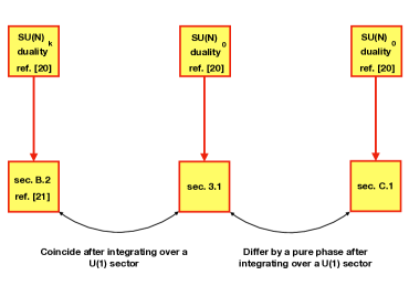
Figure 1: The various real mass flows leading to the $[p,q]$ case studied in this paper and their relation. We report the references corresponding to the UV duality where the RG flows considered here start.

Figure 2: The various real mass flows leading to the $[p,0]$ case studied in this paper and their relation. We report the references corresponding to the UV duality where the RG flows considered here start.

Figure 3: The various real mass flows leading to the $[p,q]^{*}$ case studied in this paper and their relation. We report the references corresponding to the UV duality where the RG flows considered here start.

4 Dualities for $U(N_{c})$ chiral adjoint SQCD

In this section we extend the chiral dualities of Benini:2011mf to $U(N_{c})$ gauge theories with adjoint matter. Again we can distinguish three cases, identified by the relative size of $\Delta F$ with respect to the CS level $2k$. In order to furnish a uniform picture we once again borrow the notation of Benini:2011mf , and distinguish the three classes $[p,q]_{\text{adj}}$, $[p,0]_{\text{adj}}$, and $[p,q]_{\text{adj}}^{*}$, where the subscript adj denotes the presence of an adjoint multiplet. Actually the last two cases analyzed in this section have already been studied in Hwang:2015wna , while the third case has not appear in the literature yet (to the best of the authors’ knowledge).

Let us first state the duality in the non-chiral case Kim:2013cma (see also Nii:2014jsa ). The electric theory is 3d $\mathcal{N}=2$ $U(N_{c})$ SQCD, with $N_{f}$ pairs of fundamentals $Q$ and antifundamentals $\tilde{Q}$ and one adjoint $X$. There is a superpotential

$$W=\operatorname{Tr}X^{n+1}\ .$$ (31)

The fields are charged under the various symmetries as follows:

$$\begin{array}[]{c|cccccc}&U(N_{c})&SU(N_{f})_{L}&SU(N_{f})_{R}&U(1)_{T}&U(1)_{A}&U(1)_{R}\\ \hline\cr Q&\mathbf{N}_{c}&\mathbf{N}_{f}&\mathbf{1}&0&1&\Delta\\ \tilde{Q}&\overline{\mathbf{N}_{c}}&\mathbf{1}&\overline{\mathbf{N}_{f}}&0&1&\Delta\\ X&\mathbf{Adj}&\mathbf{1}&\mathbf{1}&0&0&\frac{2}{n+1}\\ \end{array}$$ (32)

The dual theory is 3d $\mathcal{N}=2$ $U(nN_{f}-N_{c})$ SQCD, with $N_{f}$ pairs of dual fundamentals $q$ and dual antifundamentals $\tilde{q}$ and one adjoint $Y$. There are also $nN_{f}^{2}$ singlets $M_{j}=QX^{j}\tilde{Q}$ with $j=0,\dots,n-1$, corresponding to the (dressed) mesons, which are non-vanishing in the chiral ring of the electric theory, and $2n$ singlets $T_{j,+}=T_{+}X^{j}$ and $T_{j,-}=T_{-}X^{j}$ with $j=0,\dots,n-1$, corresponding to the (dressed) monopoles and antimonopoles (respectively) of the electric theory acting as singlets in the magnetic phase. The dual superpotential is

$$W=\operatorname{Tr}Y^{n+1}+\sum_{j=0}^{n-1}(M_{j}qY^{j}\tilde{q}+T_{j,+}t_{n-1-j,-}+T_{j,-}t_{n-1-j,+})\ .$$ (33)

The fields are charged under the various symmetries as follows:

$$\begin{array}[]{c|cccccc}&U(\widetilde{N}_{c})&SU(N_{f})_{L}&SU(N_{f})_{R}&U(1)_{T}&U(1)_{A}&U(1)_{R}\\ \hline\cr\rule{0.0pt}{15.0pt}q&\widetilde{\mathbf{N}}_{c}&\overline{\mathbf{N}_{f}}&\mathbf{1}&0&-1&\frac{2}{k+1}-\Delta\\ \tilde{q}&\overline{\widetilde{\mathbf{N}}_{c}}&\mathbf{1}&\mathbf{N}_{f}&0&-1&\frac{2}{k+1}-\Delta\\ Y&\mathbf{Adj}&\mathbf{1}&\mathbf{1}&0&0&\frac{2}{k+1}\\ M_{j}&\mathbf{1}&\mathbf{N}_{f}&\overline{\mathbf{N}_{f}}&0&2&2\Delta+\frac{2j}{k+1}\\ T_{j,+}&\mathbf{1}&\mathbf{1}&\mathbf{1}&1&-N_{f}&N_{f}(1-\Delta)-\frac{2}{k+1}(N_{c}-1-j)\\ T_{j,-}&\mathbf{1}&\mathbf{1}&\mathbf{1}&-1&-N_{f}&N_{f}(1-\Delta)-\frac{2}{k+1}(N_{c}-1-j)\\ \end{array}$$ (34)

The equivalence between the electric and the magnetic partition function was discussed in Amariti:2014iza and corresponds to the identity

$$Z_{\text{ele}}^{U(N_{c})}(\tau;\mu;\nu;\lambda)= \ \prod_{j=0}^{n-1}\Gamma_{h}\left(\pm\frac{\lambda}{2}-\frac{1}{2}\sum(\mu_{a}+\nu_{a})+\tau(j-N_{c}+1)+\omega N_{f}\right)$$

$$\cdot\prod_{a,b=1}^{N_{f}}\Gamma_{h}(\mu_{a}+\nu_{b}+j\omega\tau)\cdot Z_{\text{mag}}^{U(nN_{f}-N_{c})}(\tau;\tau-\nu;\tau-\mu;-\lambda)$$ (35)

where the partition function of a $U(N_{c})$ gauge theory with an adjoint and $N_{f}$ pairs of fundamentals and antifundamentals is

$$Z^{U(N_{c})}(\tau;\mu;\nu;\lambda)= \ \frac{\Gamma_{h}(\tau)^{N_{c}}}{N_{c}!}\int\prod_{i=1}^{N_{c}}d\sigma_{i}\prod_{i<j}\frac{\Gamma_{h}(\tau\pm(\sigma_{i}-\sigma_{j}))}{\Gamma_{h}(\pm(\sigma_{i}-\sigma_{j}))}e^{i\pi\lambda\sum_{i}\sigma_{i}}\cdot$$

$$\cdot\prod_{i=1}^{N_{c}}\left(\prod_{a=1}^{N_{f}}\Gamma_{h}(\mu_{a}+\sigma_{i})\cdot\Gamma_{h}(\nu_{a}-\sigma_{i})\right)\ .$$ (36)

The mass parameters are $\mu_{a}\equiv m_{A}+m_{a}$ and $\nu_{a}\equiv m_{A}+n_{a}$, and are constrained by $\sum_{a=1}^{N_{f}}m_{a}=\sum_{a=1}^{N_{f}}n_{a}=0$. Moreover the superpotential (31) imposes $\tau=\frac{2}{n+1}\omega$.

A comment regarding the identity (4) is in order. That relation was obtained in Amariti:2014iza by reducing the identity between the electric and the magnetic side of the 4d Kutasov–Schwimmer–Seiberg duality Kutasov:1995ve ; Kutasov:1995np ; Kutasov:1995ss , i.e. by reducing the superconformal index of each side and equating the two. As is customary for many superconformal index identities, its existence was not established rigorously, although several hints towards the existence of such a relation were furnished in Spiridonov:2009za . Furthermore in Dolan:2008qi a perturbative proof was discussed at large $N_{c}$ at fixed $N_{f}$. Here we will assume (4) holds.

The chiral dualities in the classes $[p,q]_{\text{adj}}$, $[p,0]_{\text{adj}}$, and $[p,q]_{\text{adj}}^{*}$ can be obtained by studying the real mass flows analogous to the ones formulated in Benini:2011mf . Again we study these three cases separately.

4.1 $\Delta F<2k$: the $[p,q]_{\mathrm{adj}}$ case

In this case we assign a positive large real mass to $N_{f}-N_{f}^{(1)}$ fundamentals and a positive large real mass to $N_{f}-N_{f}^{(2)}$ antifundamentals. The electric theory is $U(N_{c})_{k}$ with $N_{f}^{(1)}$ fundamentals and $N_{f}^{(2)}$ antifundamentals. The CS level generated by this real mass flow is $k=N_{f}-\tfrac{1}{2}(N_{f}^{(1)}+N_{f}^{(2)})$ and $\Delta F=|N_{f}^{(1)}-N_{f}^{(2)}|<2k=2N_{f}-N_{f}^{(1)}-N_{f}^{(2)}$. The dual gauge group is $U(nN_{f}-N_{c})_{-k}$, with $N_{f}^{(1)}$ antifundamentals and $N_{f}^{(2)}$ fundamentals. The (dressed) monopoles and antimonopoles acting as singlets in the dual phase are massive and we integrate them out. We are left with the superpotential

$$W=\operatorname{Tr}Y^{n+1}+\sum_{j=0}^{n-1}M_{j}qY^{j}\tilde{q}\ .$$ (37)

The real mass flow just described can be reproduced on the three-sphere partition function. This corresponds to assigning the following mass parameters:

$$\left\{\begin{array}[]{l l l l l}m_{A}&\to&m_{A}-s\frac{N_{f}^{(1)}+N_{f}^{(2)}-2N_{f}}{2N_{f}};&\\ m_{a}&\to&m_{a}+s\frac{N_{f}^{(1)}-N_{f}}{2N_{f}},&a=1,\dots,N_{f}^{(1)};\\ m_{a}&\to&m_{a}+s\frac{N_{f}^{(1)}}{2N_{f}},&a=N_{f}^{(1)}+1,\dots,N_{f}-N_{f}^{(1)};\\ n_{a}&\to&n_{a}+s\frac{N_{f}^{(2)}-N_{f}}{2N_{f}},&a=1,\dots,N_{f}^{(2)};\\ n_{a}&\to&n_{a}+s\frac{N_{f}^{(2)}}{2N_{f}},&a=N_{f}^{(2)}+1,\dots,N_{f}-N_{f}^{(2)};\\ \sigma_{i}&\to&\sigma_{i}-s\frac{N_{f}^{(1)}-N_{f}^{(2)}}{2N_{f}},&i=1,\dots,N_{c};\\ \tilde{\sigma}_{i}&\to&\tilde{\sigma}_{i}-s\frac{N_{f}^{(1)}-N_{f}^{(2)}}{2N_{f}},&i=1,\dots,nN_{f}-N_{c};\\ \lambda&\to&\lambda+s\big{(}N_{f}^{(1)}-N_{f}^{(2)}\big{)}&\end{array}\right.$$ (38)

The real mass flow consists of studying the large $s$ limit on both sides of the identity (4). The divergent contributions cancel between the electric and the magnetic phase and we obtain a new identity $Z_{\text{ele}}=Z_{\text{mag}}$ that reproduces the duality discussed above. The electric partition function is

$$Z_{\text{ele}}= \ \frac{\Gamma_{h}(\tau)^{N_{c}}}{N_{c}!}\int\prod_{i=1}^{N_{c}}d\sigma_{i}\prod_{i<j}\frac{\Gamma_{h}(\tau\pm(\sigma_{i}-\sigma_{j}))}{\Gamma_{h}(\pm(\sigma_{i}-\sigma_{j}))}\,e^{-i\pi k\sum_{i}\sigma_{i}(\sigma_{i}-\hat{\lambda})}\cdot$$

$$\cdot\prod_{i=1}^{N_{c}}\left(\prod_{a=1}^{N_{f}^{(1)}}\Gamma_{h}(\mu_{a}+\sigma_{i})\cdot\prod_{b=1}^{N_{f}^{(2)}}\Gamma_{h}(\nu_{a}-\sigma_{i})\right)\ ,$$ (39)

with

$$\hat{\lambda}\equiv\lambda+(N_{f}^{(1)}-N_{f}^{(2)})(m_{A}-\omega)\ .$$ (40)

The magnetic one is

$$Z_{\text{mag}}= \ \frac{e^{i\pi\phi}\Gamma_{h}(\tau)^{\widetilde{N}_{c}}}{\widetilde{N}_{c}!}\prod_{a=1}^{N_{f}^{(1)}}\prod_{b=1}^{N_{f}^{(2)}}\Gamma_{h}(\mu_{a}+\nu_{b}+j\omega\tau)\cdot$$

$$\int\prod_{i=1}^{\widetilde{N}_{c}}d\sigma_{i}\prod_{i<j}\frac{\Gamma_{h}(\tau\pm(\sigma_{i}-\sigma_{j}))}{\Gamma_{h}(\pm(\sigma_{i}-\sigma_{j}))}\,e^{\frac{i\pi}{4}\lambda^{2}n}e^{i\pi k\sum_{i}\sigma_{i}(\sigma_{i}-\tilde{\lambda})}$$

$$\cdot\prod_{i=1}^{\widetilde{N}_{c}}\left(\prod_{a=1}^{N_{f}^{(1)}}\Gamma_{h}(\tau-\mu_{a}-\sigma_{i})\cdot\prod_{b=1}^{N_{f}^{(2)}}\Gamma_{h}(\tau-\nu_{a}+\sigma_{i})\right)\ ,$$ (41)

with

$$\tilde{\lambda}\equiv\lambda+(N_{f}^{(1)}-N_{f}^{(2)})(m_{A}-\tau+\omega)$$ (42)

The complex exponent $\phi$ reads

$$\phi= -\frac{1}{2}\bigg{\{}\frac{1}{2}n\bigg{[}(N_{f}^{(1)}-N_{f}^{(2)}+2k)\sum_{a=1}^{N_{f}^{(1)}}m_{a}^{2}+(N_{f}^{(2)}-N_{f}^{(1)}+2k)\sum_{b=1}^{N_{f}^{(2)}}n_{b}^{2}\bigg{]}+$$

$$+m_{A}\bigg{[}\frac{1}{2}(N_{f}^{(2)}+N_{f}^{(1)})(N_{f}^{(2)}+N_{f}^{(1)}+2k)(nm_{A}+2((n-2)\omega+\tau))+$$

$$-4N_{f}^{(2)}N_{f}^{(1)}(nm_{A}+\tau-2\omega)+2N_{c}(N_{f}^{(2)}+N_{f}^{(1)})(\tau-2\omega)\bigg{]}\bigg{\}}+$$

$$+n\tau\bigg{\{}\frac{\tau}{2}\big{[}(\widetilde{N}_{c}^{2}+(N_{f}^{(1)}-N_{c})(N_{f}^{(2)}-N_{c}))-\frac{(n-1)^{2}}{8}(N_{f}^{(2)}+N_{f}^{(1)}+2k)\cdot$$

$$\cdot(N_{f}^{(2)}+N_{f}^{(1)})\big{]}-\frac{n-1}{12}\omega\big{[}\frac{1}{4}(N_{f}^{(2)}+N_{f}^{(1)}+2k)^{2}-N_{f}^{(1)}N_{f}^{(2)}-2\big{]}\bigg{\}}\ .$$ (43)

4.2 $\Delta F=2k$: the $[p,0]_{\mathrm{adj}}$ case

In this case we assign a positive large real mass to $N_{f}-N_{f}^{(1)}$ fundamentals. The electric theory is $U(N_{c})_{k}$ with $N_{f}^{(1)}$ fundamentals and $N_{f}$ antifundamentals. The CS level generated by this real mass flow is $k=\tfrac{1}{2}(N_{f}-N_{f}^{(1)})$ and $\Delta F=N_{f}-N_{f}^{(1)}=2k$. The dual gauge group is $U(nN_{f}-N_{c})_{-k}$, with $N_{f}^{(1)}$ antifundamentals and $N_{f}$ fundamentals. The (dressed) monopoles acting as singlets in the dual phase are massive and we integrate them out. On the other hand the antimonopoles remain massless because the shift due to the large mass is compensated by a shift of the FI. The dual superpotential is

$$W=\operatorname{Tr}Y^{n+1}+\sum_{j=0}^{n-1}M_{j}qY^{j}\tilde{q}+{T}_{j,-}t_{n-1-j,+}\ .$$ (44)

Equivalently we can assign a positive large real mass to $N_{f}-N_{f}^{(2)}$ antifundamentals, this latter case being related to the former by a parity transformation. The difference is that the last term in the dual superpotential (44) becomes ${T}_{j,-}t_{n-1-j,+}$.

The real mass flow just described can be reproduced on the three-sphere partition function. This corresponds to assigning the following mass parameters:

$$\left\{\begin{array}[]{l l l l }m_{A}&\to&m_{A}+s\frac{N_{f}-N_{f}^{(1)}}{2N_{f}};&\\ m_{a}&\to&m_{a}-s\frac{N_{f}-N_{f}^{(1)}}{N_{f}},&a=1,\dots,N_{f}^{(1)};\\ m_{a}&\to&m_{a}+s\frac{N_{f}^{(1)}}{N_{f}},&a=N_{f}^{(1)}+1,\dots,N_{f};\\ \sigma_{i}&\to&\sigma_{i}+s\frac{N_{f}-N_{f}^{(1)}}{2N_{f}},&i=1,\dots,N_{c};\\ \tilde{\sigma}_{i}&\to&\tilde{\sigma}_{i}+s\frac{N_{f}-N_{f}^{(1)}}{2N_{f}},&i=1,\dots,nN_{f}-N_{c};\\ \lambda&\to&\lambda+s(N_{f}-N_{f}^{(1)}).&\end{array}\right.$$ (45)

The real mass flow consists of studying the large $s$ limit on both sides of the identity (4). The divergent contributions cancel between the electric and the magnetic phase and we obtain a new identity $Z_{\text{ele}}=Z_{\text{mag}}$ that reproduces the duality discussed above. The electric partition function is

$$Z_{\text{ele}}= \ \frac{\Gamma_{h}(\tau)^{N_{c}}}{N_{c}!}\int\prod_{i=1}^{N_{c}}d\sigma_{i}\prod_{i<j}\frac{\Gamma_{h}(\tau\pm(\sigma_{i}-\sigma_{j}))}{\Gamma_{h}(\pm(\sigma_{i}-\sigma_{j}))}\,e^{-i\pi k\sum_{i}\sigma_{i}(\sigma_{i}-\hat{\lambda})}\cdot$$

$$\cdot\prod_{i=1}^{N_{c}}\left(\prod_{a=1}^{N_{f}^{(1)}}\Gamma_{h}(\mu_{a}+\sigma_{i})\cdot\prod_{b=1}^{N_{f}}\Gamma_{h}(\nu_{a}-\sigma_{i})\right)\ ,$$ (46)

with

$$\hat{\lambda}\equiv\lambda-\big{(}N_{f}-N_{f}^{(1)}\big{)}(m_{A}-\omega)\ .$$ (47)

The magnetic one is

$$Z_{\text{mag}}= \ \frac{e^{\frac{i\pi}{2}n\phi}\Gamma_{h}(\tau)^{\widetilde{N}_{c}}}{\widetilde{N}_{c}!}\prod_{a=1}^{N_{f}^{(1)}}\prod_{b=1}^{N_{f}}\Gamma_{h}(\mu_{a}+\nu_{b}+j\omega\tau)$$

$$\int\prod_{i=1}^{\widetilde{N}_{c}}d\tilde{\sigma}_{i}\prod_{i<j}\frac{\Gamma_{h}(\tau\pm(\tilde{\sigma}_{i}-\tilde{\sigma}_{j}))}{\Gamma_{h}(\pm(\tilde{\sigma}_{i}-\tilde{\sigma}_{j}))}\,e^{-i\pi k\sum_{i}\tilde{\sigma}_{i}(\tilde{\sigma}_{i}+\tilde{\lambda})}\cdot$$

$$\cdot\prod_{i=1}^{\widetilde{N}_{c}}\left(\prod_{a=1}^{N_{f}^{(1)}}\Gamma_{h}(\tau-\mu_{a}-\tilde{\sigma}_{i})\cdot\prod_{b=1}^{N_{f}}\Gamma_{h}(\tau-\nu_{a}+\tilde{\sigma}_{i})\right)\ ,$$ (48)

with

$$\tilde{\lambda}\equiv\ \lambda-\big{(}N_{f}-N_{f}^{(1)}\big{)}(m_{A}-\tau+\omega)\ .$$ (49)

The complex exponent $\phi$ reads

$$\phi= \ N_{f}(N_{f}^{(1)}-4k)m_{A}^{2}-\frac{\omega}{3}\bigg{[}\tau-\omega+(N_{f}^{(1)}+2k)(10k(\tau-\omega)-3N_{f}^{(1)}\omega)\bigg{]}-2k\sum_{b=1}^{N_{f}}n_{b}^{2}+$$

$$+2m_{A}(2k\tau N_{f}+N_{f}^{(1)}\tau N_{c}-\omega N_{f})+N_{c}\tau((N_{f}-N_{f}^{(1)}+N_{c})\tau-2\omega N_{f})\ .$$ (50)

4.3 $\Delta F>2k$: the $[p,q]_{\mathrm{adj}}^{*}$ case

This is the case that has not been discussed in Hwang:2015wna . In this case one assigns a positive mass to $N_{f}^{(1)}$ antifundamentals and a negative mass to $N_{f}^{(2)}$ antifundamentals. The CS level is $k=\tfrac{1}{2}(N_{f}^{(1)}-N_{f}^{(2)})$ and $\Delta F=N_{f}^{(1)}+N_{f}^{(2)}>2k\equiv N_{f}^{(1)}-N_{f}^{(2)}$. The electric theory is $U(N_{c})_{k}$ with $N_{f}$ fundamentals and $N_{a}$ antifundamentals with $N_{a}=N_{f}-N_{f}^{(1)}-N_{f}^{(2)}$. The dual gauge group is $U(nN_{f}-N_{c})_{-k}$ with $N_{a}$ fundamentals and $N_{f}$ antifundamentals. The (dressed) monopoles and antimonopoles acting as singlets in the dual phase are massive and we integrate them out. We are left with the dual superpotential

$$W=\operatorname{Tr}Y^{n+1}+\sum_{j=0}^{n-1}M_{j}qY^{j}\tilde{q}\ .$$ (51)

By a parity transformation one can also obtain the case where $N_{f}<N_{a}$. In general one has an electric $U(N_{c})_{k}$ theory with $N_{f}$ fundamentals, $N_{a}$ antifundamentals, and $|N_{f}-N_{a}|>2k$, dual to $U(n\,\max(N_{f},N_{a})-N_{c})_{-k}$ with $N_{f}$ dual antifundamentals, $N_{a}$ dual fundamentals, and the superpotential (51).

The real mass flow just described can be reproduced on the three-sphere partition function. This corresponds to assigning the following mass parameters:

$$\left\{\begin{array}[]{l l l l }m_{A}&\to&m_{A}+s\frac{N_{f}^{(1)}-N_{f}^{(2)}}{N_{f}};&\\ n_{a}&\to&n_{a}-s\frac{N_{f}^{(1)}-N_{f}^{(2)}}{N_{f}},&a=1,\dots,N_{a};\\ n_{a}&\to&n_{a}+s\frac{N_{f}-N_{f}^{(1)}+N_{f}^{(2)}}{N_{f}},&a=N_{a}+1,\dots,N_{a}+N_{f}^{(2)}=N_{f}-N_{f}^{(1)};\\ n_{a}&\to&n_{a}-s\frac{N_{f}+N_{f}^{(1)}-N_{f}^{(2)}}{N_{f}},&a=N_{a}+N_{f}^{(2)}+1,\dots,N_{f};\\ \sigma_{i}&\to&\sigma_{i}-s\frac{N_{f}^{(1)}-N_{f}^{(2)}}{N_{f}},&i=1,\dots,N_{c};\\ \tilde{\sigma}_{i}&\to&\tilde{\sigma}_{i}-s\frac{N_{f}^{(1)}-N_{f}^{(2)}}{N_{f}};&i=1,\dots,nN_{f}-N_{c},\\ \lambda&\to&\lambda-s(N_{f}^{(1)}+N_{f}^{(2)});&\end{array}\right.$$ (52)

The real mass flow consists of studying the large $s$ limit on both sides of the identity (4). The divergent contributions cancel between the electric and the magnetic phase and we obtain a new identity $Z_{\text{ele}}=Z_{\text{mag}}$ that reproduces the duality discussed above. The electric partition function is

$$Z_{\text{ele}}= \ \frac{\Gamma_{h}(\tau)^{N_{c}}}{N_{c}!}\int\prod_{i=1}^{N_{c}}d\sigma_{i}\prod_{i<j}\frac{\Gamma_{h}(\tau\pm(\sigma_{i}-\sigma_{j}))}{\Gamma_{h}(\pm(\sigma_{i}-\sigma_{j}))}\,e^{-i\pi k\sum_{i}\sigma_{i}(\sigma_{i}-\hat{\lambda})}\cdot$$

$$\prod_{i=1}^{N_{c}}\left(\prod_{a=1}^{N_{f}}\Gamma_{h}(\mu_{a}+\sigma_{i})\cdot\prod_{b=1}^{N_{a}}\Gamma_{h}(\nu_{a}-\sigma_{i})\right)\ ,$$ (53)

with

$$\hat{\lambda}\equiv\lambda-2k(m_{A}-\omega)\ .$$ (54)

The magnetic one is

$$Z_{\text{mag}}= \ \frac{e^{i\pi nk\phi}\Gamma_{h}(\tau)^{\widetilde{N}_{c}}}{\widetilde{N}_{c}!}e^{i\pi\lambda n\left(\tau N_{c}-N_{f}\left(\omega-m_{A}\right)\right)}\prod_{a=1}^{N_{f}}\prod_{b=1}^{N_{a}}\Gamma_{h}(\mu_{a}+\nu_{b}+j\omega\tau)\cdot$$

$$\int\prod_{i=1}^{\widetilde{N}_{c}}d\tilde{\sigma}_{i}\prod_{i<j}\frac{\Gamma_{h}(\tau\pm(\tilde{\sigma}_{i}-\tilde{\sigma}_{j}))}{\Gamma_{h}(\pm(\tilde{\sigma}_{i}-\tilde{\sigma}_{j}))}\,e^{i\pi k\sum_{i}\tilde{\sigma}_{i}(\tilde{\sigma}_{i}-\tilde{\lambda})}\cdot$$

$$\cdot\prod_{i=1}^{\widetilde{N}_{c}}\left(\prod_{a=1}^{N_{f}}\Gamma_{h}(\tau-\mu_{a}-\tilde{\sigma}_{i})\cdot\prod_{b=1}^{N_{a}}\Gamma_{h}(\tau-\nu_{a}+\tilde{\sigma}_{i})\right)\ ,$$ (55)

with

$$\tilde{\lambda}\equiv\lambda-2k(m_{A}-\tau+\omega)\ .$$ (56)

The complex exponent $\phi$ reads

$$\phi=\tau N_{c}\left(\tau-2m_{A}\right)-N_{f}\left(3m_{A}^{2}-2m_{A}(\tau+\omega)-\frac{1}{3}(n-4)\tau\omega\right)-\sum_{a=1}^{N_{f}}m_{a}^{2}\ .$$ (57)

5 Dualities for $SU(N_{c})$ chiral adjoint SQCD

In this section we generalize the construction to the case of $SU(N_{c})$ SQCD with $N_{f}$ flavors $Q$ and $\tilde{Q}$ and an adjoint $X$, interacting through the superpotential in (31). The dual model was derived in Park:2013wta (see also Nii:2014jsa ). It is a $U(nN_{f}-N_{c})\times U(1)$ gauge theory with $N_{f}$ flavors $q$ and $\tilde{q}$ in the nonabelian sector, and $n$ pairs $(T_{j,+},T_{j,-}$ (with $j=0,\dots,n-1$) of opposite gauge charge in the $U(1)$ gauge sector. These latter fields interact through the superpotential with the dressed monopoles $t_{i,+}$ and antimonopoles $t_{i,-}$ of the $U(nN_{f}-N_{c})$ sector. Such monopoles and antimonopoles carry charge $-1$ and $+1$ (respectively) under the $U(1)$ gauge group as well. The superpotential of the dual gauge theory is

$$W=\operatorname{Tr}Y^{n+1}+\sum_{j=0}^{n-1}M_{j}qY^{j}\tilde{q}+T_{j,+}t_{n-1-j,-}+T_{j,-}t_{n-1-j,+}\ ,$$ (58)

where $M_{j}=QX^{j}\tilde{Q}$ are the $nN_{f}^{2}$ dressed mesons of the electric theory acting as singlets in the dual phase. There is also a level-$1$ mixed CS term between the abelian center $U(1)\subset U(nN_{f}-N_{c})$ and the other $U(1)$ gauge factor.

The fields are charged under the various symmetries as follows:

$$\begin{array}[]{c|cccccc}&SU(N_{c})&SU(N_{f})_{L}&SU(N_{f})_{R}&U(1)_{B}&U(1)_{A}&U(1)_{R}\\ \hline\cr Q&\mathbf{N}_{c}&\mathbf{N}_{f}&\mathbf{1}&1&1&\Delta\\ \tilde{Q}&\overline{\mathbf{N}_{c}}&\mathbf{1}&\overline{\mathbf{N}_{f}}&-1&1&\Delta\\ X&\mathbf{Adj}&\mathbf{1}&\mathbf{1}&0&0&\frac{2}{n+1}\\ \end{array}$$ (59)

The dual model is a $U(\widetilde{N}_{c})\times U(1)$ gauge theory, with a mixed CS term between $U(1)\subset U(\widetilde{N}_{c})$ and the other $U(1)$ gauge symmetry. The fields are charged under the various symmetries as follows:

$$\begin{array}[]{c|cccccc}&U(\widetilde{N}_{c})\times U(1)&SU(N_{f})_{L}&SU(N_{f})_{R}&U(1)_{B}&U(1)_{A}&U(1)_{R}\\ \hline\cr\rule{0.0pt}{15.0pt}q&\widetilde{\mathbf{N}}_{c,0}&\overline{\mathbf{N}_{f}}&\mathbf{1}&0&-1&1-\Delta\\ \tilde{q}&\overline{\widetilde{\mathbf{N}}_{c}}_{,0}&\mathbf{1}&\mathbf{N}_{f}&0&-1&1-\Delta\\ Y&\mathbf{Adj}_{0}&\mathbf{1}&\mathbf{1}&0&0&\frac{2}{n+1}\\ M_{j}&\mathbf{1}_{0}&\mathbf{N}_{f}&\overline{\mathbf{N}_{c}}&0&2&2\left(\Delta+\frac{j}{n+1}\right)\\ T_{j,+}&\mathbf{1}_{1}&\mathbf{1}&\mathbf{1}&N_{c}&N_{f}&N_{f}(1-\Delta)+\frac{2(j-N_{c}+1)}{n+1}\\ T_{j,-}&\mathbf{1}_{-1}&\mathbf{1}&\mathbf{1}&-N_{c}&N_{f}&N_{f}(1-\Delta)+\frac{2(j-N_{c}+1)}{n+1}\\ \end{array}$$ (60)

The duality for $SU(N_{c})$ adjoint SQCD can be represented at the level of the partition function, by manipulating the identity (4). We first multiply the partition function by a factor $\frac{1}{2}e^{-i\pi\lambda N_{c}m_{B}}$. Then we gauge the topological symmetry, i.e. we integrate over $\lambda$. By shifting $\sigma_{i}\rightarrow\sigma_{i}+m_{B}$ we produce a factor $\delta(\sigma_{1}+\dots+\sigma_{N_{c}})$. The partition function of the electric theory then becomes

$$Z_{\text{ele}}= \ \frac{\Gamma_{h}(\tau)^{N_{c}}}{N_{c}!}\int\prod_{i=1}^{N_{c}}d\sigma_{i}\,\delta\left(\sum_{i=1}^{N_{c}}\sigma_{i}\right)\prod_{i<j}\frac{\Gamma_{h}(\tau\pm(\sigma_{i}-\sigma_{j}))}{\Gamma_{h}(\pm(\sigma_{i}-\sigma_{j}))}\cdot$$

$$\cdot\prod_{i=1}^{N_{c}}\left(\prod_{a=1}^{N_{f}}\Gamma_{h}(\mu_{a}+\sigma_{i}+m_{B})\cdot\Gamma_{h}(\nu_{a}-\sigma_{i}-m_{B})\right)\ .$$ (61)

On the dual side the theory is $U(nN_{f}-N)\times U(1)$, and there is a mixed CS term between the two $U(1)$s. The partition function is then

$$Z_{\text{mag}}= \ \frac{\Gamma_{h}(\tau)^{\widetilde{N}_{c}}}{\widetilde{N}_{c}!}\,\prod_{j=0}^{n-1}\prod_{a,b=1}^{N_{f}}\Gamma_{h}(\mu_{a}+\nu_{b}+j\omega\tau)\cdot$$

$$\int d\xi\prod_{j=0}^{n-1}\Gamma_{h}\left(\pm\xi-\frac{1}{2}\sum(\mu_{a}+\nu_{a})+\tau(j-N_{c}+1)+\omega N_{f}\right)\cdot$$

$$\int\prod_{i=1}^{\widetilde{N}_{c}}d\tilde{\sigma}_{i}\prod_{i<j}\frac{\Gamma_{h}(\tau\pm(\tilde{\sigma}_{i}-\tilde{\sigma}_{j}))}{\Gamma_{h}(\pm(\tilde{\sigma}_{i}-\tilde{\sigma}_{j}))}\,e^{-2i\pi\xi\sum_{i}(\tilde{\sigma}_{i}+\frac{N_{c}}{nN_{f}-N_{c}}m_{B})}\cdot$$

$$\cdot\prod_{i=1}^{nN_{f}-N_{c}}\left(\prod_{a=1}^{N_{f}}\Gamma_{h}(\tau-\mu_{a}-\tilde{\sigma}_{i})\Gamma_{h}(\tau-\nu_{a}+\tilde{\sigma}_{i})\right)\ .$$ (62)

We can shift $\tilde{\sigma}_{i}$ in the magnetic partition function and define a more canonical baryonic symmetry. Again, in order to have a proper charge normalization for the fields in the $U(1)$ sector we have used the substitution $\lambda=2\xi$ in (4).

The equivalence between (5) and (5) corresponds to the duality of Park:2013wta at the level of the partition function. Observe that in both cases there is an overall factor $\Gamma_{h}(\tau)^{\operatorname{rk}(G)}$, where $\operatorname{rk}(G)$ is $N_{c}$ on the electric and $\widetilde{N}_{c}=nN_{f}-N_{c}$ on the dual side. Actually, in the final identity, because we are dealing with an $SU(N_{c})$ gauge group on the electric side the rank is rather given by $\operatorname{rk}(G)=N_{c}-1$. On the dual side this corresponds to considering a new singlet $\beta$ and a superpotential coupling $W\propto\beta\,\operatorname{Tr}Y$. By integrating out the massive fields we are left with the overall contribution $\Gamma_{h}(\tau)^{\widetilde{N}_{c}-1}$ on the magnetic side, that corresponds to a traceleness requirement for the adjoint of the dual gauge group. Equivalently on the dual side we consider the adjoint of the $SU(\widetilde{N}_{c})\subset U(\widetilde{N}_{c})$ subgroup.

In the following, starting from the identity between (5) and (5), we consider the three different real mass flows that correspond to the three generalizations of $[p,q]_{\text{adj}}^{*}$, $[p,0]_{\text{adj}}$ and $[p,q]_{\text{adj}}$.

5.1 $\Delta F<2k$: $SU$ generalization of the $[p,q]_{\mathrm{adj}}$ case

In this case the real mass flow generalizes the one studied in section 3.1. We assign a positive large real mass to $N_{f}-N_{f}^{(1)}$ fundamentals and a positive large real mass to $N_{f}-N_{f}^{(2)}$ antifundamentals. The electric theory is $SU(N_{c})_{k}$ adjoint SQCD with $N_{f}^{(1)}$ fundamentals and $N_{f}^{(2)}$ antifundamentals. The CS level generated by this real mass flow is $k=N_{f}-\tfrac{1}{2}(N_{f}^{(1)}+N_{f}^{(2)})$ and $\Delta F=|N_{f}^{(1)}-N_{f}^{(2)}|<2k=2N_{f}-N_{f}^{(1)}-N_{f}^{(2)}$.

On the dual we must consider a nonzero vacuum for the scalar in the vector multiplet and we must shift the scalar in the vector multiplet of the gauged topological symmetry. We are left with $U\big{(}n(\tfrac{1}{2}(N_{f}^{(1)}+N_{f}^{(2)})+k)-N_{c}\big{)}_{-k}\times U(1)_{-n}$ gauge symmetry with a mixed CS level, at level $1$, between the two $U(1)$ symmetries. There are $N_{f}^{(1)}$ dual antifundamentals and $N_{f}^{(2)}$ dual fundamentals and there is a superpotential

$$W=\operatorname{Tr}Y^{n+1}+\sum_{j=0}^{n-1}M_{j}qY^{j}\tilde{q}\ .$$ (63)

The real mass flow just described corresponds to the assignment (12) followed by a large $s$ limit. Defining $\mu_{a}\equiv m_{a}+m_{A}+m_{B}$ and $\nu_{a}\equiv n_{a}+m_{A}-m_{B}$ we have

$$Z_{\text{ele}}= \ \frac{1}{N_{c}!}\int\prod_{i=1}^{N_{c}}d\sigma_{i}\,e^{-i\pi k\sum_{i}\sigma_{i}^{2}}\,\delta\left(\sum_{i=1}^{N_{c}}\sigma_{i}\right)\prod_{i<j}\frac{\Gamma_{h}(\tau\pm(\sigma_{i}-\sigma_{j}))}{\Gamma_{h}(\pm(\sigma_{i}-\sigma_{j}))}\,\cdot$$

$$\cdot\prod_{i=1}^{N_{c}}\left(\prod_{a=1}^{N_{f}^{(1)}}\Gamma_{h}(\mu_{a}+\sigma_{i})\cdot\prod_{b=1}^{N_{f}^{(2)}}\Gamma_{h}(\nu_{a}-\sigma_{i})\right)\ .$$ (64)

The magnetic partition function is

$$Z_{\text{mag}}= \ \frac{e^{i\pi\phi}}{\widetilde{N}_{c}!}\prod_{j=0}^{n-1}\prod_{a=1}^{N_{f}^{(1)}}\prod_{b=1}^{N_{f}^{(2)}}\Gamma_{h}(\mu_{a}+\nu_{b}+j\omega\tau)\int d\xi e^{i\pi(n\xi^{2}+2\xi m_{B}N_{c})}\cdot$$

$$\int\prod_{i=1}^{\widetilde{N}_{c}}d\sigma_{i}\,e^{i\pi(k\sum_{i}\tilde{\sigma}_{i}^{2}+2(\xi-\eta)\sum_{i}\tilde{\sigma}_{i})}\,\prod_{i<j}\frac{\Gamma_{h}(\tau\pm(\tilde{\sigma}_{i}-\tilde{\sigma}_{j}))}{\Gamma_{h}(\pm(\tilde{\sigma}_{i}-\tilde{\sigma}_{j}))}\,\cdot$$

$$\cdot\prod_{i=1}^{\widetilde{N}_{c}}\left(\prod_{a=1}^{N_{f}^{(1)}}\Gamma_{h}(\tau-\mu_{a}-\tilde{\sigma}_{i})\cdot\prod_{b=1}^{N_{f}^{(2)}}\Gamma_{h}(\tau-\nu_{b}+\tilde{\sigma}_{i})\right)\ ,$$ (65)

where

$$\eta\equiv\frac{N_{f}^{(1)}-N_{f}^{(2)}}{2}(m_{A}-\tau+\omega)\ .$$ (66)

The complex exponent $\phi$ reads

$$\phi= \ \frac{n}{4}\bigg{[}(2k+N_{f}^{(1)}-N_{f}^{(2)})\sum_{a=1}^{N_{f}^{(1)}}m_{a}^{2}+(2k-N_{f}^{(1)}+N_{f}^{(2)})\sum_{b=1}^{N_{f}^{(2)}}n_{b}^{2}\bigg{]}-kN_{c}m_{B}^{2}+$$

$$+N_{c}m_{A}m_{B}(N_{f}^{(1)}-N_{f}^{(2)})+\frac{nm_{A}}{4}\bigg{\{}(n-1)\tau\big{[}N_{f}^{(1)}(N_{f}^{(1)}+2k)+N_{f}^{(2)}(N_{f}^{(2)}+2k)\big{]}+$$

$$-4N_{c}\tau(N_{f}^{(1)}+N_{f}^{(2)})+4(\tau+\omega)N_{f}^{(1)}N_{f}^{(2)}\bigg{\}}+\frac{nm_{A}^{2}}{4}\bigg{\{}2k(N_{f}^{(1)}+N_{f}^{(2)})-6N_{f}^{(1)}N_{f}^{(2)}+$$

$$+{N_{f}^{(1)}}^{2}+{N_{f}^{(2)}}^{2}\bigg{\}}-N_{c}\omega m_{B}(N_{f}^{(1)}-N_{f}^{(2)})-\frac{n\tau}{24}\bigg{\{}3\tau\bigg{[}n^{2}(N_{f}^{(1)}+N_{f}^{(2)}+2k)^{2}+$$

$$-\frac{1}{2}(N_{f}^{(1)}+N_{f}^{(2)}+2k)((n-1)^{2}(N_{f}^{(1)}+N_{f}^{(2)})+8nN_{c})-4N_{c}(N_{f}^{(1)}+N_{f}^{(2)})+$$

$$+4N_{f}^{(1)}N_{f}^{(2)}+8N_{c}^{2}\bigg{]}+2\omega(n-1)\bigg{[}N_{f}^{(1)}N_{f}^{(2)}+2-\frac{1}{4}(N_{f}^{(1)}+N_{f}^{(2)}+2k)^{2}\bigg{]}\bigg{\}}\ .$$ (67)

5.2 $\Delta F=2k$: $SU$ generalization of the $[p,0]_{\mathrm{adj}}$ case

In this case the real mass flow generalizes the one studied in section 3.2. We assign a positive large real mass to $N_{f}-N_{f}^{(1)}$ antifundamentals. The electric theory is $SU(N_{c})_{k}$ adjoint SQCD with $N_{f}$ fundamentals and $N_{f}^{(1)}$ antifundamentals and superpotential $W=\operatorname{Tr}X^{n+1}$ The CS level generated by this real mass flow is $k=\tfrac{1}{2}(N_{f}-N_{f}^{(1)})$ and $\Delta F=|N_{f}-N_{f}^{(1)}|=2k$. On the magnetic side we take again a nonzero vacuum for the scalar in the vector multiplet, and we shift the scalar in the vector multiplet of the gauged topological symmetry. We are left with $U\big{(}\widetilde{N}_{c}\equiv n\big{(}k+\tfrac{1}{2}(N_{f}+N_{f}^{(1)})\big{)}-N_{c}\big{)}_{-k}\times U(1)_{-\frac{n}{2}}$ gauge symmetry with a mixed CS level, at level $1$, between the $U(1)$ symmetries. In the $U(1)$ sector the fields $T_{j,-}$ are massive and are integrated out. The fields $T_{j,+}$ are massless, because the shift induced by real masses is canceled against the one of the real scalar of the gauged topological $U(1)$. In the $U(\widetilde{N}_{c})$ sector there are also $N_{f}$ dual antifundamentals and $N_{f}^{(1)}$ dual fundamentals. The dual superpotential is

$$W=\operatorname{Tr}Y^{n+1}+\sum_{j=0}^{n-1}M_{j}qY^{j}\tilde{q}+T_{j,+}\,t_{n-1-j,-}\ .$$ (68)

The real mass flow corresponds to the assignment (18), followed by a large $s$ limit. The electric partition function is

$$Z_{\text{ele}}= \ \frac{1}{N_{c}!}\int\prod_{i=1}^{N_{c}}d\sigma_{i}\,e^{-i\pi k\sum_{i}\sigma_{i}^{2}}\,\delta\left(\sum_{i=1}^{N_{c}}\sigma_{i}\right)\prod_{i<j}\frac{\Gamma_{h}(\tau\pm(\sigma_{i}-\sigma_{j}))}{\Gamma_{h}(\pm(\sigma_{i}-\sigma_{j}))}\,\cdot$$

$$\cdot\prod_{i=1}^{N_{c}}\left(\prod_{a=1}^{N_{f}}\Gamma_{h}(\mu_{a}+\sigma_{i}+m_{B})\cdot\prod_{b=1}^{N_{f}^{(1)}}\Gamma_{h}(\nu_{a}-\sigma_{i}-m_{B})\right)\ .$$ (69)

The magnetic one is

$$Z_{\text{mag}}= \ \frac{e^{i\pi\phi}}{\widetilde{N}_{c}!}\prod_{j=0}^{n-1}\prod_{a=1}^{N_{f}}\prod_{b=1}^{N_{f}^{(1)}}\Gamma_{h}(\mu_{a}+\nu_{b}+j\omega\tau)\cdot$$

$$\int d\xi e^{\frac{i\pi}{2}n\xi^{2}+i\pi\xi(nN_{f}(\omega-m_{A})+N_{c}(2m_{B}+n\tau))}\prod_{j=0}^{n-1}\Gamma_{h}((\omega-m_{A})N_{f}-\xi+\tau(j-N_{c}+1))\cdot$$

$$\int\prod_{i=1}^{\widetilde{N}_{c}}d\tilde{\sigma}_{i}\,e^{i\pi(k\sum_{i}\tilde{\sigma}_{i}^{2}+2(\xi-\eta)\sum_{i}\tilde{\sigma}_{i})}\,\prod_{i<j}\frac{\Gamma_{h}(\tau\pm(\tilde{\sigma}_{i}-\tilde{\sigma}_{j}))}{\Gamma_{h}(\pm(\tilde{\sigma}_{i}-\tilde{\sigma}_{j}))}\,\cdot$$

$$\cdot\prod_{i=1}^{\widetilde{N}_{c}}\left(\prod_{a=1}^{N_{f}}\Gamma_{h}(\tau-\mu_{a}-\tilde{\sigma}_{i})\cdot\prod_{b=1}^{N_{f}^{(1)}}\Gamma_{h}(\tau-\nu_{b}+\tilde{\sigma}_{i})\right)\ ,$$ (70)

with

$$\eta\equiv k\left(m_{A}-\tau+\omega\right)\ .$$ (71)

The complex exponent $\phi$ reads

$$\phi= \ n(N_{f}^{(1)}-N_{f})\sum_{a=1}^{N_{f}}m_{a}^{2}-2\eta(nN_{f}(m_{A}-\omega)+N_{c}(m_{B}+n\tau))\ +$$

$$+N_{f}^{(1)}(nN_{f}(m_{A}-\omega)^{2}-N_{c}(m_{B}+n\tau)^{2})+N_{f}N_{c}(2n\tau(m_{A}+m_{B})+m_{B}^{2})\ +$$

$$+n\tau(\tau N_{c}(N_{c}-N_{f})-\frac{1}{6}(N_{f}(N_{f}-N_{f}^{(1)})-1)(n-1)\omega)\ .$$ (72)

5.3 $\Delta F>2k$: $SU$ generalization of the $[p,q]_{\mathrm{adj}}^{*}$ case

In this case the real mass flow generalizes the one studied in section 3.3. We assign a positive large real mass to $N_{f}^{(1)}$ antifundamentals and a negative large real mass to $N_{f}^{(2)}$ antifundamentals. The electric theory is $SU(N_{c})_{k}$ with $N_{f}$ fundamentals and $N_{a}$ antifundamentals with $N_{a}=N_{f}-N_{f}^{(1)}-N_{f}^{(2)}$. The CS level generated by this real mass flow is $k=\frac{1}{2}(N_{f}^{(1)}-N_{f}^{(2)})$ and $\Delta F=N_{f}-N_{a}=N_{f}^{(1)}+N_{f}^{(2)}>2k=N_{f}^{(1)}-N_{f}^{(2)}$. On the magnetic side we need to consider a nonzero vacuum for the scalar in the vector multiplet and we also need to shift the scalar in the vector multiplet of the gauged topological symmetry. We are left with $U(nN_{f}-N_{c})_{-k}\times U(1)_{0}$ gauge symmetry with a mixed CS level, at level $1$, between the two $U(1)$ symmetries. In the $U(1)$ sector obtained by gauging the topological symmetry all the fields $T_{j,\pm}$ are massive. In the $U(\widetilde{N}_{c})$ sector there are $N_{f}$ dual antifundamentals and $N_{a}$ dual fundamentals and there is a superpotential

$$W=\operatorname{Tr}Y^{n+1}+\sum_{j=0}^{n-1}M_{j}qY^{j}\tilde{q}\ .$$ (73)

By a parity transformation one can also define the case where $N_{f}<N_{a}$. In general one has an electric $SU(N_{c})_{k}$ theory with $N_{f}$ fundamentals, $N_{a}$ antifundamentals, and $|N_{f}-N_{a}|>2k$, dual to $(U(n\max(N_{f},N_{a})-N_{c})_{-k}\times U(1)_{0})_{1}$ with $N_{f}$ dual antifundamentals, $N_{a}$ dual fundamentals, and the superpotential (73).

The real mass flow corresponds to the assignment (26) , followed by a large $s$ limit: The electric partition function is

$$Z_{\text{ele}}= \ \frac{1}{N_{c}!}\int\prod_{i=1}^{N_{c}}d\sigma_{i}\,e^{-i\pi k\sum_{i}\sigma_{i}^{2}}\,\delta\left(\sum_{i=1}^{N_{c}}\sigma_{i}\right)\prod_{i<j}\frac{\Gamma_{h}(\tau\pm(\sigma_{i}-\sigma_{j}))}{\Gamma_{h}(\pm(\sigma_{i}-\sigma_{j}))}\,\cdot$$

$$\cdot\prod_{i=1}^{N_{c}}\left(\prod_{a=1}^{N_{f}}\Gamma_{h}(\mu_{a}+\sigma_{i}+m_{B})\prod_{b=1}^{N_{f}-N_{f}^{(1)}-N_{f}^{(2)}}\Gamma_{h}(\nu_{b}-\sigma_{i}-m_{B})\right)\ .$$ (74)

The magnetic one is

$$Z_{\text{mag}}= \ \frac{e^{i\pi\phi}}{\widetilde{N}_{c}!}\prod_{j=0}^{n-1}\prod_{a=1}^{N_{f}}\prod_{b=1}^{N_{f}-N_{f}^{(1)}-N_{f}^{(2)}}\Gamma_{h}(\mu_{a}+\nu_{b}+j\omega\tau)\int d\xi\,e^{2i\pi\xi(nN_{f}(m_{A}-\omega)+N_{c}(m_{B}+n\tau))}$$

$$\cdot\prod_{i=1}^{\widetilde{N}_{c}}d\tilde{\sigma}_{i}\,e^{i\pi(k\sum_{i}\tilde{\sigma}_{i}^{2}+2i\pi(\xi-\eta)\sum_{i}\tilde{\sigma}_{i})}\,\prod_{i<j}\frac{\Gamma_{h}(\tau\pm(\tilde{\sigma}_{i}-\tilde{\sigma}_{j}))}{\Gamma_{h}(\pm(\tilde{\sigma}_{i}-\tilde{\sigma}_{j}))}\,\cdot$$

$$\cdot\prod_{i=1}^{\widetilde{N}_{c}}\left(\prod_{a=1}^{N_{f}}\Gamma_{h}(\tau-\mu_{a}-\tilde{\sigma}_{i})\cdot\prod_{b=1}^{N_{f}-N_{f}^{(1)}-N_{f}^{(2)}}\Gamma_{h}(\tau-\nu_{a}+\tilde{\sigma}_{i})\right)\ ,$$ (75)

with

$$\eta\equiv k(m_{A}+\omega-\tau)\ .$$ (76)

The complex exponent $\phi$ reads

$$\phi= \ k\bigg{\{}N_{c}(\tau-2m_{A}+m_{B})(n\tau+m_{B})-n\sum_{a=1}^{N_{f}}m_{a}^{2}\ +$$

$$+nN_{f}\bigg{[}m_{A}((n+3)\tau-m_{A})+\frac{(n-4)}{3}\tau\omega\bigg{]}\bigg{\}}\ .$$ (77)

6 Conclusions

In this paper we have provided a full classification of 3d $\mathcal{N}=2$ dualities for adjoint SQCD with unitary and special unitary gauge group and a different amount of fundamentals $N_{f}$ and antifundamentals $N_{a}$. The classification generalizes the construction of Benini:2011mf for $U(N_{c})$ SQCD and the one of Aharony:2014uya ; Nii:2020xgd for $SU(N_{c})$ SQCD. It distinguishes three cases, depending on the relative value of the difference $\Delta F=|N_{f}-N_{a}|$ with respect to the CS level $k$. We have kept the notation of Benini:2011mf where the $\Delta F<2k$ case is denoted $[p,q]$, $\Delta F=2k$ is denoted $[p,0]$, and $\Delta F>2k$ is denoted $[p,q]^{*}$. The analysis of Benini:2011mf was performed starting from the original case of Aharony duality, where $N_{f}=N_{a}$ and the CS level is vanishing, and subsequently applying a real mass flow to produce chiral dualities. The dualities were corroborated by an analysis of the flow at the level of three-sphere partition functions (i.e. by matching them across dual phases). Here we have derived chiral dualities for $SU(N_{c})$ SQCD starting from the $SU(N_{c})$ version of Aharony duality (i.e. at zero CS level). This is different from the analysis of Aharony:2014uya where the starting point was the generalization of Giveon–Kutasov duality for $SU(N_{c})_{k}$ SQCD. We have commented in appendix B on the relation between the two approaches. In this way we have also studied the flow of Aharony:2014uya on the three-sphere partition function. Then we have extended our analysis of chiral dualities to the case of adjoint SQCD. We have considered the non-chiral dualities for $U(N_{c})$ and $SU(N_{c})$ adjoint SQCD of Nii:2014jsa ; Amariti:2014iza and performed the real mass flow on the corresponding integral identities between three-sphere partition functions. In this way we have obtained a complete classification. Notice that one can further simplify the integral identities of section 5 by performing the $\xi$ integral (corresponding to the $U(1)$ gauge sector). The analysis in the $[p,q]_{\text{adj}}$ and $[p,q]^{*}_{\text{adj}}$ is straightforward (one performs a gaussian integral in the former and uses identity (8) in the latter), analogously to what done in section 3. The $[p,0]_{\text{adj}}$ case is more complex because the $\xi$ integral corresponds to $U(1)_{-n/2}$ with $n$ negatively charged fields, which is not (known to be) dual to a set of singlets.

As a bonus, we have obtained integral identities for $U(N_{c})$ CS matter theories where the CS level of the $SU(N_{c})$ factor differs from the one of the $U(1)$ factor. These types of integrals have not been thoroughly investigated so far, but they can be interesting for checking e.g. the dualities recently studied in Nii:2020ikd .

Further checks and generalizations of our analysis are possible. For instance it would be desirable to match the moduli space between the dual phases, extending the analysis of Nii:2014jsa to the case of adjoint SQCD. Another independent check of the dualities that we have constructed here consists of computing the superconformal indices of the dual phases, and matching them at least for small rank $N_{c}$.

It could also be possible to obtain the chiral dualities for adjoint SQCD studied in section 4 starting from the non-chiral dualities at nonzero CS level discussed in Niarchos:2008jb ; Niarchos:2009aa ; Kapustin:2011vz . In such a case the electric theory corresponds to $U(N_{c})_{k}$ SQCD with $N_{f}$ pairs of fundamentals and antifundamentals $Q$ and $\tilde{Q}$ and an adjoint $X$ with superpotential $W=\operatorname{Tr}X^{n+1}$, while the dual model is $U(n(N_{f}+|k|)-N_{c})_{-k}$ SQCD with $N_{f}$ pairs of fundamentals and antifundamentals, an adjoint $Y$ and $nN_{f}$ singlets $M_{j}=QX^{j}\tilde{Q}$, with superpotential

$$W=\operatorname{Tr}Y^{n+1}+\sum_{j=0}^{n-1}M_{j}qY^{j}\tilde{q}\ .$$ (78)

The relevant integral identities to match the partition functions were given in Amariti:2014iza . The $SU(N_{c})$ version of this duality can be obtained by gauging the topological symmetry and it can be used to also reproduce the dualities studied in section 5.

Other chiral dualities can be derived from the non-chiral ones of Giacomelli:2017vgk ; Giacomelli:2019blm and of Pasquetti:2019tix : the latter case is interesting because the integral identities needed to match the three-sphere partition functions are known. Another possibility would be constructing chiral dualities for SQCD with two adjoints (which is studied in Hwang:2018uyj ).

Appendix A $SU(N_{c})_{k_{1}}\times U(1)_{k_{2}}$ and the partition function

In order to compare the results obtained here with the ones discussed in Aharony:2014uya ; Nii:2020xgd , it is necessary to distinguish the values of the CS levels of the $SU(N_{c})$ and the $U(1)$ factor of $U(N_{c})=(SU(N_{c})\times U(1))/\mathbb{Z}_{N_{c}}$. In general we have obtained here CS contributions to the partition function of the form

$$\exp\left[-i\pi k_{1}\sum_{i=1}^{N_{c}}\sigma_{i}^{2}-i\pi k_{2}\left(\sum_{i=1}^{N_{c}}\sigma_{i}\right)^{2}\right]\ .$$ (79)

We want to isolate the $U(1)$ factor from the first term in the exponent. This can be done by redefining $\sigma_{i}=\frac{x_{0}}{\sqrt{N_{c}}}-x_{i}$ with $x_{1}+\dots+x_{N_{c}}=0$. In this way (79) becomes

$$\delta\left(\sum_{i=1}^{N_{c}}x_{i}\right)\exp\left[-i\pi k_{1}\sum_{i=1}^{N_{c}}x_{i}^{2}-i\pi\left(k_{1}+N_{c}k_{2}\right)x_{0}^{2}\right]\ ,$$ (80)

i.e. we have shown that (79) corresponds to the CS contribution to the partition function of the gauge group $U(N_{c})_{k_{1},k_{1}+N_{c}k_{2}}$, where $k_{1}$ is the CS level of the $SU(N_{c})$ factor (with eigenvalues $\{x_{i}\}_{i=1}^{N_{c}}$) and $k_{1}+N_{c}k_{2}$ is the CS level of the $U(1)$ factor (with eigenvalue $x_{0}$).

Appendix B The flow of Aharony:2014uya on the partition function

In this section we discuss the real mass flow from the $SU(N)_{k}$ Giveon–Kutasov duality presented in (Aharony:2013dha, , Eq. (3.23)) to the chiral dualities. This is the flow originally considered in Aharony:2014uya and here we study this flow as an infinite limit on the real masses on the partition function. The starting point is the identity between the electric $SU(N)_{k}$ (for $k>0$) theory with $N_{f}$ pairs of fundamentals and antifundamentals and its $U(N_{f}-N_{c}+k)_{-k,N_{f}-N_{c}}$ dual with $N_{f}$ pairs of dual fundamentals and antifundamentals and superpotential $W=Mq\tilde{q}$. Up to our knowledge the integral identity relating these two phases has not appeared in the literature so far: for this reason we start our analysis by deriving such an identity by gauging the topological symmetry of Giveon–Kutasov duality. Then we study the $[p,q]$, $[p,0]$, and $[p,q]^{*}$ cases separately, comparing the relations obtained here with the ones discussed in the section 3.

B.1 Integral identity for $SU(N_{c})_{k}$ duality

Our starting point is the identity

$$Z_{U(N_{c})_{k}}(\mu;\nu;2\xi)=\prod_{a,b=1}^{N_{f}}\Gamma_{h}(\mu_{a}+\nu_{b})Z_{U(N_{f}-N_{c}+k)_{-k}}(\omega-\nu;\omega-\mu;-2\xi)\ .$$ (81)

We then add a term $e^{2i\pi m_{B}\xi}$ on both sides and gauge the topological symmetry by integrating over $\xi$. We arrive at the identity $Z_{\text{ele}}=Z_{\text{mag}}$ with

$$Z_{\text{ele}}= \ \frac{1}{N_{c}!}\int\prod_{i=1}^{N_{c}}d\sigma_{i}\,\delta\left(\sum_{i=1}^{N_{c}}\sigma_{i}\right)\prod_{i<j}\Gamma_{h}(\pm(\sigma_{i}-\sigma_{j}))^{-1}\,e^{-i\pi k\left(m_{B}^{2}N_{c}+\sum_{i}\sigma_{i}^{2}\right)}\cdot$$

$$\cdot\prod_{i=1}^{N_{c}}\left(\prod_{a=1}^{N_{f}}\Gamma_{h}(\mu_{a}+m_{B}+\sigma_{i})\Gamma_{h}(\nu_{a}-m_{B}-\sigma_{i})\right)\ ,$$ (82)

$$Z_{\text{mag}}= \ \frac{e^{-\frac{i\pi}{2}\phi}}{\widetilde{N}_{c}!}\prod_{a,b=1}^{N_{f}}\Gamma_{h}(\mu_{a}+\nu_{b})\int\prod_{i=1}^{\widetilde{N}_{c}}d\tilde{\sigma}_{i}e^{i\pi\left(k\sum_{i}\tilde{\sigma}_{i}^{2}-\left(N_{c}m_{B}-\sum_{i}\tilde{\sigma}_{i}\right)^{2}\right)}$$

$$\cdot\prod_{i=1}^{\widetilde{N}_{c}}\left(\prod_{a=1}^{N_{f}}\Gamma_{h}(\omega-\mu_{a}-\tilde{\sigma}_{i})\Gamma_{h}(\omega-\nu_{a}+\tilde{\sigma}_{i})\right)\prod_{i<j}{\Gamma_{h}(\pm(\tilde{\sigma}_{i}-\tilde{\sigma}_{j}))}^{-1}\ .$$ (83)

The complex exponent $\phi$ reads

$$\phi= \ k\sum_{a=1}^{N_{f}}\left(m_{a}^{2}+n_{a}^{2}\right)+2\omega\widetilde{N}_{c}\left(k\omega-2m_{A}N_{f}\right)\ +$$

$$-4k\omega m_{A}N_{f}+2m_{A}^{2}N_{f}(k-N_{f})-2\omega^{2}\widetilde{N}_{c}^{2}-k^{2}\omega^{2}\ .$$ (84)

The dual partition function in (B.1) coincides with the one obtained in (3.1).

B.2 $\Delta F<2k$

Here we study the flow of Aharony:2014uya corresponding the the $\Delta F<2k$, i.e. $[p,q]$ case. In this case the real mass flow corresponds to shifting the mass parameters appearing in the partition function as follows:

$$\left\{\begin{array}[]{llll}m_{A}&\to&m_{A}-s\frac{N_{f}^{(m)}}{2N_{f}};&\\ m_{B}&\to&m_{B}-s\frac{N_{f}^{(m)}}{2N_{f}};&\\ m_{a}&\to&m_{a}-s\frac{\left(N_{f}-N_{f}^{(m)}\right)}{N_{f}},&a=1,\dots,N_{f}^{(m)};\\ m_{a}&\to&m_{a}+s\frac{N_{f}^{(m)}}{N_{f}},&a=N_{f}^{(m)}+1,\dots,N_{f}-N_{f}^{(m)}\end{array}\right.$$ (85)

with $s>0$. On the magnetic side we also shift $\sigma$ by a term $-s\frac{N_{f}^{(m)}}{2N_{f}}$. After canceling the infinite contributions, that coincide on the electric and magnetic side, we obtain the identity $Z_{\text{ele}}=Z_{\text{mag}}$, where

$$Z_{\text{ele}}= \ \frac{1}{N_{c}!}\int\prod_{i=1}^{N_{c}}d\sigma_{i}\,\delta\left(\sum_{i=1}^{N_{c}}\sigma_{i}\right)\prod_{i<j}\Gamma_{h}(\pm(\sigma_{i}-\sigma_{j}))^{-1}\,e^{-i\pi\left(k+\tfrac{1}{2}N_{f}^{(m)}\right)\sum_{i}\sigma_{i}^{2}}\cdot$$

$$\cdot\prod_{i=1}^{N_{c}}\left(\prod_{a=1}^{N_{f}-N_{f}^{(m)}}\Gamma_{h}(\mu_{a}+m_{B}+\sigma_{i})\prod_{a=1}^{N_{f}}\Gamma_{h}(\nu_{a}-m_{B}-\sigma_{i})\right)\ ,$$ (86)

and

$$Z_{\text{mag}}= \ \frac{e^{-\frac{i\pi}{2}\phi}}{\widetilde{N}_{c}!}\prod_{a=1}^{N_{f}-N_{f}^{(m)}}\prod_{b=1}^{N_{f}}\Gamma_{h}(\mu_{a}+\nu_{b})\int\prod_{i=1}^{\widetilde{N}_{c}}d\tilde{\sigma}_{i}\,e^{i\pi\left(\eta\sum_{i}\tilde{\sigma}_{i}+\left(k+\tfrac{1}{2}N_{f}^{(m)}\right)\sum_{i}\tilde{\sigma}_{i}^{2}-\left(\sum_{i}\tilde{\sigma}_{i}\right)^{2}\right)}\cdot$$

$$\cdot\prod_{a=1}^{N_{f}-N_{f}^{(m)}}\Gamma_{h}(\omega-\mu_{a}-\tilde{\sigma}_{i})\prod_{a=1}^{N_{f}}\Gamma_{h}(\omega-\nu_{a}+\tilde{\sigma}_{i})\prod_{i<j}\frac{1}{\Gamma_{h}(\pm(\tilde{\sigma}_{i}-\tilde{\sigma}_{j}))}\ ,$$ (87)

with $\widetilde{N}_{c}\equiv N_{f}-N_{c}+k$ and $\eta\equiv 2N_{c}m_{B}-N_{f}m_{A}$. The complex exponent $\phi$ reads

$$\phi= -k\sum_{a=1}^{N_{f}-N_{f}^{(m)}}m_{a}^{2}-(N_{f}^{(m)}+k)\sum_{b=1}^{N_{f}}n_{b}^{2}+N_{c}\left[2m_{B}(m_{A}-\omega)N_{f}^{(m)}+\right.$$

$$+\left.\omega((\omega-2m_{A})N_{f}^{(m)}-4N_{f}(\omega-m_{A})-2k\omega)+m_{B}^{2}(N_{f}^{(m)}+2k)\right]\ +$$

$$+N_{f}(\omega-m_{A})\left[m_{A}(3N_{f}^{(m)}+2k)+km_{A}^{2}N_{f}^{(m)}+2N_{f}^{2}(\omega-m_{A})^{2}+\right.$$

$$+\left.2N_{c}^{2}(\omega^{2}-m_{B}^{2})+k^{2}\omega^{2}+\omega(2k-N_{f}^{(m)})\right]\ .$$ (88)

It is straightforward to prove that this result coincides with the one obtained in section 3.1 upon using the dictionary

$$\{N_{f},N_{f}^{(m)},k\}_{\text{here}}=\{N_{f}^{(2)},N_{f}^{(2)}-N_{f}^{(1)},N_{f}-N_{f}^{(2)}\}_{\text{sec.}\,\ref{pqPP}}\ .$$ (89)

B.3 $\Delta F=2k$

The $\Delta F=2k$, $[p,0]$ case is obtained by studying the above flow with $s<0$ and $N_{f}^{(m)}=k$. Actually the analysis of Aharony:2014uya for $s<0$ was performed in the whole range $N_{f}^{(m)}\leq k$. In this case one considers the real masses

$$\left\{\begin{array}[]{llll}m_{A}&\to&m_{A}-s\frac{N_{f}^{(m)}}{2N_{f}};&\\ m_{B}&\to&m_{B}-s\frac{N_{f}^{(m)}}{2N_{f}};&\\ m_{a}&\to&m_{a}-s\frac{\left(N_{f}-N_{f}^{(m)}\right)}{N_{f}},&a=1,\dots,N_{f}^{(m)};\\ m_{a}&\to&m_{a}+s\frac{N_{f}^{(m)}}{N_{f}},&a=N_{f}^{(m)}+1,\dots,N_{f}-N_{f}^{(m)}.\end{array}\right.$$ (90)

In the dual phase the shift on the scalar in the vector multiplet breaks the gauge symmetry as well. Explicitly, the shift is given by

$$\left\langle\tilde{\sigma}\right\rangle\to\begin{bmatrix}\tilde{\sigma}_{(N_{f}-N_{c})\times(N_{f}-N_{c})}&0\\ 0&\theta_{k\times k}\end{bmatrix}-s\begin{bmatrix}\left(\frac{N_{f}^{(m)}}{2N_{f}}\right)\mathbf{1}_{N_{f}-N_{c}}&0\\ 0&\left(\frac{N_{f}^{(m)}}{2N_{f}}-1\right)\mathbf{1}_{k}\end{bmatrix}\ ,$$ (91)

where $\mathbf{1}_{n}$ denotes the $n\times n$ identity matrix. In this case the divergent phase does not cancel in general between the electric and the magnetic side. In effect, we are left with a term $e^{-2i\pi s(N_{f}^{(m)}-k)\varphi}$ where

$$\varphi=N_{f}^{(m)}(m_{A}-\omega)+\sum_{j=0}^{k}\theta_{j}\ .$$ (92)

For $N_{f}^{(m)}<k$ we expect that the divergent term is balanced by a shift in the FI due to the VEV acquired by the dual fundamentals needed to solve the D-term equation (3.9) of Aharony:2014uya . Such a shift can be expected to arise from the Higgs branch localization Fujitsuka:2013fga ; Benini:2013yva . Following the discussion of Fujitsuka:2013fga one can see that the Higgsing does not affect the one-loop determinants of the chiral fields while it affects the contribution from the classical action. This naive argument supports the fact that the dual model is equivalent to the $[p,q]$ one discussed above.

On the other hand the term (92) cancels out when $N_{f}^{(m)}=k$. In such a case we arrive at the identity $Z_{\text{ele}}=Z_{\text{mag}}$, where

$$Z_{\text{ele}}= \ \frac{1}{N_{c}!}\int\prod_{i=1}^{N_{c}}d\sigma_{i}\,\delta\left(\sum_{i=1}^{N_{c}}\sigma_{i}\right)\prod_{i<j}\Gamma_{h}(\pm(\sigma_{i}-\sigma_{j}))^{-1}\,e^{-i\pi\frac{k}{2}\sum_{i}\sigma_{i}^{2}}\cdot$$

$$\cdot\prod_{i=1}^{N_{c}}\left(\prod_{a=1}^{N_{f}-k}\Gamma_{h}(\mu_{a}+m_{B}+\sigma_{i})\prod_{a=1}^{N_{f}}\Gamma_{h}(\nu_{a}-m_{B}-\sigma_{i})\right)\ ,$$ (93)

and

$$Z_{\text{mag}}= \ \frac{e^{\frac{i\pi}{2}\phi}}{(N_{f}-N_{c})!k!}\prod_{a=1}^{N_{f}-k}\prod_{b=1}^{N_{f}}\Gamma_{h}(\mu_{a}+\nu_{b})\int\prod_{i=1}^{N_{f}-N_{c}}d\tilde{\sigma}_{i}\prod_{j=1}^{k}d\theta_{j}$$

$$\cdot e^{i\pi\left(\frac{k}{2}\sum_{i=1}^{N_{f}-N_{c}}\tilde{\sigma}_{i}^{2}-(\sum_{i=1}^{N_{f}-N_{c}}\tilde{\sigma}_{i})^{2}\right)}\cdot$$

$$\cdot e^{i\pi\left(\frac{k}{2}\sum_{j=1}^{k}\theta_{j}^{2}-(\sum_{j=1}^{k}\theta_{j})^{2}\right)+i\pi\sum_{j=1}^{k}\theta_{j}\left(m_{A}(2N_{f}-k)-2m_{B}N_{c}-2\omega\left(N_{f}-N_{c}\right)\right)}\cdot$$

$$\cdot e^{-i\pi\sum_{i=1}^{N_{f}-N_{c}}\tilde{\sigma}_{i}\left(k\left(m_{A}-2\omega\right)+2m_{B}N_{c}\right)-2i\pi\sum_{i=1}^{N_{f}-N_{c}}\tilde{\sigma}_{i}\sum_{j=1}^{k}\theta_{i}}\cdot$$

$$\cdot\prod_{i=1}^{N_{f}-N_{c}}\left(\prod_{a=1}^{N_{f}-k}\Gamma_{h}(\omega-\mu_{a}-\tilde{\sigma}_{i})\prod_{a=1}^{N_{f}}\right)\Gamma_{h}(\omega-\nu_{a}+\tilde{\sigma}_{i})\prod_{i<j}{\Gamma_{h}(\pm(\tilde{\sigma}_{i}-\tilde{\sigma}_{j}))}^{-1}$$

$$\cdot\prod_{j=1}^{k}\prod_{a=1}^{k}\Gamma_{h}(\omega-\mu_{a}-\theta_{j})\prod_{i<j}{\Gamma_{h}(\pm(\theta_{i}-\theta_{j}))}^{-1}\ ,$$ (94)

where the $\theta_{j}$ sector corresponds to $U(k)_{-\frac{k}{2},\frac{k}{2}}$ with $k$ fundamentals. The complex exponent $\phi$ reads

$$\phi= -k\left(\sum_{a=1}^{k}m_{a}^{2}+\sum_{b=1}^{N_{f}}n_{b}^{2}\right)-kN_{c}\left(m_{B}-\omega\right)\left(2m_{A}-m_{B}-3\omega\right)+2N_{c}^{2}\left(\omega^{2}-m_{B}^{2}\right)+$$

$$+N_{f}\left(m_{A}-\omega\right)\left(k\left(m_{A}-3\omega\right)+4\omega N_{c}\right)+2N_{f}^{2}\left(m_{A}-\omega\right){}^{2}+k^{2}\left(\omega^{2}-m_{A}^{2}\right)\ .$$ (95)

In order to reproduce the $[p,0]$ dualities obtained in section 3.2 we should show that this $\theta$ sector can be dualized into a singlet. This is easily achieved for $k=1$, since $U(1)_{1/2}$ with one negatively charged field is dual to a singlet. (This is the half mirror symmetry of Dorey:1999rb we already encountered in (23).) For higher $k$ one then proceeds by dualizing one massive chiral at a time.

B.4 $\Delta F>2k$

We conclude our analysis by studying the $[p,q]^{*}$ case. In this case we consider the real masses

$$\left\{\begin{array}[]{llll}m_{A}&\to&m_{A}-s\frac{N_{f}^{(m)}}{2N_{f}};&\\ m_{B}&\to&m_{B}-s\frac{N_{f}^{(m)}}{2N_{f}};&\\ m_{a}&\to&m_{a}-s\frac{\left(N_{f}-N_{f}^{(m)}\right)}{N_{f}},&a=1,\dots,N_{f}^{(m)};\\ m_{a}&\to&m_{a}+s\frac{N_{f}^{(m)}}{N_{f}},&a=N_{f}^{(m)}+1,\dots,N_{f},\end{array}\right.$$ (96)

with $s<0$ and $N_{f}^{(m)}<k$. In the dual phase the shift on the scalar in the vector multiplet breaks the gauge symmetry as well. Explicitly the shift is

$$\left\langle\tilde{\sigma}\right\rangle\to\begin{bmatrix}\tilde{\sigma}_{(N_{f}-N_{c})\times(N_{f}-N_{c})}&0\\ 0&\theta_{k\times k}\end{bmatrix}+s\begin{bmatrix}\left(\frac{N_{f}^{(m)}}{2N_{f}}\right)\mathbf{1}_{N_{f}-N_{c}}&0\\ 0&\left(\frac{N_{f}^{(m)}}{2}\left(\frac{1}{N_{f}}-\frac{2}{k}\right)\right)\mathbf{1}_{k}\end{bmatrix}\ ,$$ (97)

In this case the divergent phase cancel between the electric and the magnetic side and we are left with the identity $Z_{\text{ele}}=Z_{\text{mag}}$, where

$$Z_{\text{ele}}= \ \frac{1}{N_{c}!}\int\prod_{i=1}^{N_{c}}d\sigma_{i}\,\delta\left(\sum_{i=1}^{N_{c}}\sigma_{i}\right)\prod_{i<j}\Gamma_{h}(\pm(\sigma_{i}-\sigma_{j}))^{-1}\,e^{-i\pi\left(k-\tfrac{1}{2}N_{f}^{(m)}\right)\sum_{i}\sigma_{i}^{2}}\cdot$$

$$\cdot\prod_{i=1}^{N_{c}}\left(\prod_{a=1}^{N_{f}-N_{f}^{(m)}}\Gamma_{h}(\mu_{a}+m_{B}+\sigma_{i})\prod_{a=1}^{N_{f}}\Gamma_{h}(\nu_{a}-m_{B}-\sigma_{i})\right)\ ,$$ (98)

and

$$Z_{\text{mag}}= \ \frac{e^{\frac{i\pi}{2}\phi}}{(N_{f}-N_{c})!k!}\prod_{a=1}^{N_{f}-N_{f}^{(m)}}\prod_{b=1}^{N_{f}}\Gamma_{h}(\mu_{a}+\nu_{b})\int\prod_{i=1}^{\widetilde{N}_{c}}d\tilde{\sigma}_{i}\prod_{j=1}^{k}d\theta_{j}\prod_{1\leq i<j\leq k}\frac{1}{\Gamma_{h}(\pm(\theta_{i}-\theta_{j}))}$$

$$\cdot\prod_{1\leq i<j\leq\widetilde{N}_{c}}\frac{1}{\Gamma_{h}(\pm(\tilde{\sigma}_{i}-\tilde{\sigma}_{j}))}\,e^{i\pi\left(\left(k-\tfrac{1}{2}N_{f}^{(m)}\right)\sum_{i=1}^{N_{f}-N_{c}}\tilde{\sigma}_{i}^{2}-(\sum_{i=1}^{N_{f}-N_{c}}\tilde{\sigma}_{i})^{2}\right)}\cdot$$

$$\cdot e^{i\pi\left(k\sum_{j=1}^{k}\theta_{j}^{2}-(\sum_{j=1}^{k}\theta_{j})^{2}\right)+2i\pi\sum_{j=1}^{k}\theta_{i}\left(N_{f}(m_{A}-\omega)-N_{c}(m_{B}-\omega)\right)}\cdot$$

$$\cdot e^{-i\pi\sum_{i=1}^{N_{f}-N_{c}}\tilde{\sigma}_{i}\left(N_{f}^{(m)}m_{A}-2k\omega+2m_{B}N_{c}\right)-2i\pi\sum_{i=1}^{N_{f}-N_{c}}\tilde{\sigma}_{i}\sum_{j=1}^{k}\theta_{i}}\cdot$$

$$\cdot\prod_{i=1}^{\widetilde{N}_{c}}\left(\prod_{a=1}^{N_{f}-N_{f}^{(m)}}\Gamma_{h}(\omega-\mu_{a}-\tilde{\sigma}_{i})\prod_{a=1}^{N_{f}}\Gamma_{h}(\omega-\nu_{a}+\tilde{\sigma}_{i})\right)\ ,$$ (99)

The complex exponent $\phi$ reads

$$\phi= \ (N_{f}^{(m)}-k)\sum_{b=1}^{N_{f}}n_{b}^{2}-k\sum_{a=1}^{N_{f}}m_{a}^{2}-N_{c}N_{f}^{(m)}\left(m_{B}-\omega\right)\left(2m_{A}+m_{B}-\omega\right)\ +$$

$$+N_{f}\left(m_{A}-\omega\right)\left[\left(3m_{A}-\omega\right)N_{f}^{(m)}-2k\left(m_{A}+\omega\right)+4\omega N_{c}\right]+2N_{f}^{2}\left(m_{A}-\omega\right)^{2}+$$

$$+2m_{B}^{2}N_{c}\left(k-N_{c}\right)\ +\omega^{2}(k^{2}-2kN_{c}+2N_{c}^{2})\ .$$ (100)

The relevant part of the partition function (B.4) that we are going to focus on is

$$\ \frac{1}{\widetilde{N}_{c}!k!}\int\prod_{i=1}^{\widetilde{N}_{c}}d\tilde{\sigma}_{i}\frac{e^{i\pi\left(k_{\text{eff}}\sum_{i}\tilde{\sigma}_{i}^{2}-\left(\sum_{i}\tilde{\sigma}_{i}\right)^{2}\right)}}{\prod_{1\leq i<j\leq\widetilde{N}_{c}}\Gamma_{h}(\pm(\tilde{\sigma}_{i}-\tilde{\sigma}_{j}))}\prod_{j=1}^{k}d\theta_{j}\prod_{1\leq i<j\leq k}\frac{1}{\Gamma_{h}(\pm(\theta_{i}-\theta_{j}))}$$

$$\cdot e^{i\pi\left(k\sum_{j=1}^{k}\theta_{j}^{2}-\left(\sum_{j=1}^{k}\theta_{j}\right)^{2}+2\rho\sum_{j=1}^{k}\theta_{i}-\eta\sum_{i=1}^{\widetilde{N}_{c}}\tilde{\sigma}_{i}-2\sum_{i=1}^{\widetilde{N}_{c}}\tilde{\sigma}_{i}\sum_{j=1}^{k}\theta_{i}\right)}\cdot$$

$$\cdot\prod_{i=1}^{\widetilde{N}_{c}}\left(\prod_{a=1}^{N_{f}^{(1)}}\Gamma_{h}(\omega-\mu_{a}-\tilde{\sigma}_{i})\prod_{a=1}^{N_{f}^{(2)}}\Gamma_{h}(\omega-\nu_{a}+\tilde{\sigma}_{i})\right)\ ,$$ (101)

with

$$k_{\text{eff}}\equiv k-\tfrac{1}{2}N_{f}^{(m)}\ ,$$ (102)

$$\rho\equiv\left(N_{f}(m_{A}-\omega)-N_{c}(m_{B}-\omega)\right)\ ,$$ (103)

$$\eta\equiv\left(N_{f}^{(m)}m_{A}-2k\omega+2m_{B}N_{c}\right)\ .$$ (104)

We can further substitute $\theta_{i}\rightarrow\xi_{i}+\frac{\xi}{k}$, with $\sum_{i=1}^{k}\xi_{i}=0$. The integral (B.4) then becomes

$$\ \frac{1}{\widetilde{N}_{c}!k!}\int\prod_{i=1}^{\widetilde{N}_{c}}d\tilde{\sigma}_{i}\prod_{j=1}^{k}\,d\xi_{i}\,\delta\left(\sum_{i=1}^{k}\xi_{i}\right)\,d\xi$$

$$e^{i\pi\left(k_{\text{eff}}\sum_{i=1}^{\widetilde{N}_{c}}\tilde{\sigma}_{i}^{2}-\left(\sum_{i=1}^{\widetilde{N}_{c}}\tilde{\sigma}_{i}\right)^{2}+k\sum_{j=1}^{k}\xi_{i}^{2}+2\rho\xi-(\eta+2\xi)\sum_{i=1}^{N}\tilde{\sigma}_{i}\right)}\cdot$$

$$\cdot\prod_{i=1}^{\widetilde{N}_{c}}\left(\prod_{a=1}^{N_{f}^{(1)}}\Gamma_{h}(\omega-\mu_{a}-\tilde{\sigma}_{i})\prod_{a=1}^{N_{f}^{(2)}}\Gamma_{h}(\omega-\nu_{a}+\tilde{\sigma}_{i})\right)\cdot$$

$$\cdot\prod_{1\leq i<j\leq\widetilde{N}_{c}}\frac{1}{\Gamma_{h}(\pm(\tilde{\sigma}_{i}-\tilde{\sigma}_{j}))}\prod_{1\leq i<j\leq k}\frac{1}{\Gamma_{h}(\pm(\xi_{i}-\xi_{j}))}\ .$$ (105)

The $\xi$ integral yields $\delta\left(\rho-\sum_{i=1}^{\widetilde{N}_{c}}\tilde{\sigma}_{i}\right)$, while the integral over $\xi_{i}$ corresponds to an $SU(k)_{-k}$ pure CS theory. Performing the latter yields $e^{\frac{i\pi}{2}k^{2}\omega^{2}}$. All in all (B.4) becomes

$$\ \frac{e^{\frac{i\pi}{2}k^{2}\omega^{2}+\frac{i\pi}{2}\phi}}{\widetilde{N}_{c}!}\int\frac{\prod_{i=1}^{\widetilde{N}_{c}}d\tilde{\sigma}_{i}}{\prod_{i<j}\Gamma_{h}(\pm(\tilde{\sigma}_{i}-\tilde{\sigma}_{j}))}\,\delta\left(\sum_{i=1}^{\widetilde{N}_{c}}\tilde{\sigma}_{i}\right)\,e^{i\pi\left(k_{\text{eff}}\sum_{i=1}^{\widetilde{N}_{c}}\tilde{\sigma}_{i}^{2}+(k_{\text{eff}}-1)\rho^{2}-\rho\eta\right)}\cdot$$

$$\cdot\prod_{i=1}^{\widetilde{N}_{c}}\left(\prod_{a=1}^{N_{f}^{(1)}}\Gamma_{h}\left(\omega-\mu_{a}-\tilde{\sigma}_{i}+\frac{\rho}{\widetilde{N}_{c}}\right)\prod_{a=1}^{N_{f}^{(2)}}\Gamma_{h}\left(\omega-\nu_{a}+\tilde{\sigma}_{i}-\frac{\rho}{\widetilde{N}_{c}}\right)\right)\ .$$ (106)

Notice that the above result coincides with (3.3) once we perform the $\xi$ integral in that formula (which yields a $\delta(\rho+\sum_{i}\sigma_{i}$)) and shift $\sigma_{i}\rightarrow\sigma_{i}-\frac{\rho}{\widetilde{N}_{c}}$:

$$Z_{\text{mag}}= \ \frac{-e^{i\pi(\frac{\phi}{2}+\frac{k\rho^{2}}{\widetilde{N}_{c}}+{\eta\rho})}}{\widetilde{N}_{c}!}\prod_{a=1}^{N_{f}}\prod_{b=1}^{N_{a}}\Gamma_{h}(\mu_{a}+\nu_{b})\int\frac{\prod_{i=1}^{\widetilde{N}_{c}}d\tilde{\sigma}_{i}}{\prod_{i<j}\Gamma_{h}(\pm({\tilde{\sigma}_{i}}-{\tilde{\sigma}_{j}}))}\delta\left(\sum_{i=1}^{\tilde{N}_{c}}\tilde{\sigma}_{i}\right)e^{i\pi{k}\sum_{i}\tilde{\sigma}_{i}^{2}}\cdot$$

$$\cdot\prod_{i=1}^{\widetilde{N}_{c}}\left(\prod_{a=1}^{N_{f}}\Gamma_{h}\left(\omega-\mu_{a}-{\tilde{\sigma}_{i}}+\frac{\rho}{\widetilde{N}_{c}}\right)\prod_{b=1}^{N_{a}}\Gamma_{h}\left(\omega-\nu_{a}+{\tilde{\sigma}_{i}}-\frac{\rho}{\widetilde{N}_{c}}\right)\right)\ .$$ (107)

We have checked that (B.4) and (B.4) are equivalent up to an irrelevant pure phase, confirming the equivalence of the $[p,q]^{*}$ case obtained in Aharony:2014uya and the one obtained here.

Appendix C $SU(N_{c})$ chiral dualities flowing from the duality of Aharony:2013dha

In this appendix we study the real mass flow in the dual models discussed in section 3 starting from the duality for $SU(N_{c})$ SQCD derived in Aharony:2013dha . In this case the dual partition function is given by formula (3). Actually here we shift the gauge symmetry by the baryonic one considering an equivalent version of the the partition function in (3):

$$Z_{\text{mag}}= \ \prod_{a,b=1}^{N_{f}}\Gamma_{h}(\mu_{a}+\nu_{b})\Gamma_{h}\left(2\omega(\widetilde{N}_{c}+1)-\sum_{a}(\mu_{a}+\nu_{a})\right)\cdot$$

$$\int\prod_{i=1}^{\widetilde{N}_{c}}d\tilde{\sigma}_{i}\prod_{i<j}\frac{1}{\Gamma_{h}(\pm(\tilde{\sigma}_{i}-\tilde{\sigma}_{j}))}\prod_{i=1}^{\widetilde{N}_{c}}\left(\prod_{a=1}^{N_{f}}\Gamma_{h}(\omega-\mu_{a}-\tilde{\sigma}_{i})\cdot\Gamma_{h}(\omega-\nu_{a}+\tilde{\sigma}_{i})\right)$$

$$\cdot\Gamma_{h}\left(\pm\left(\sum_{i=1}^{\widetilde{N}_{c}}\tilde{\sigma}_{i}+m_{B}N_{c}\right)+\frac{1}{2}\sum_{a}(\mu_{a}+\nu_{a})-\omega(N_{f}-N_{c})\right)\ .$$ (108)

Using this formula the analysis is more straightforward, because we can use the real mass flows discussed in section 3. These flows correspond to the shifts on the real masses in the partition function summarized in formulae (12), (18), and (26).

C.1 $\Delta F<2k$

In this case, by applying the flow (12) to (C) we cancel the divergent terms against the one obtained on the electric side and we are left with the finite dual magnetic partition function

$$Z_{\text{mag}}= \ e^{\frac{i\pi}{2}\phi}\prod_{a=1}^{N_{f}^{(1)}}\prod_{b=1}^{N_{f}^{(2)}}\Gamma_{h}(\mu_{a}+\nu_{b})\int\prod_{i=1}^{\widetilde{N}_{c}}d\tilde{\sigma}_{i}\,\frac{e^{-i\pi k\sum_{i}\tilde{\sigma}_{i}^{2}+i\pi\left(\sum_{i=1}^{\widetilde{N}_{c}}\tilde{\sigma}_{i}\right)^{2}-i\pi\eta_{2}\sum_{i}\tilde{\sigma}_{i}}}{\prod_{i<j}\Gamma_{h}(\pm(\tilde{\sigma}_{i}-\tilde{\sigma}_{j}))}\cdot$$

$$\cdot\prod_{i=1}^{\widetilde{N}_{c}}\left(\prod_{a=1}^{N_{f}^{(1)}}\Gamma_{h}(\omega-\mu_{a}-\tilde{\sigma}_{i})\cdot\prod_{b=1}^{N_{f}^{(2)}}\Gamma_{h}(\omega-\nu_{b}+\tilde{\sigma}_{i})\right)\ ,$$ (109)

where

$$\eta_{2}\equiv\left(N_{f}^{(1)}-N_{f}^{(2)}\right)m_{A}+2m_{B}N_{c}\ .$$ (110)

The complex exponent $\phi$ reads

$$\phi= \ m_{A}^{2}(N_{f}(N_{f}^{(1)}+N_{f}^{(2)})\!-\!4N_{f}^{(1)}N_{f}^{(2)})+m_{B}^{2}(2(N_{f}\!-\!N_{c})\!-\!(N_{f}^{(1)}+N_{f}^{(2)}))\ +$$

$$+2\left[((N_{f}^{(1)}+N_{f}^{(2)})N_{c}\!-\!2N_{f}^{(1)}N_{f}^{(2)})m_{A}+(N_{f}^{(1)}\!-\!N_{f}^{(2)})m_{B}\right]\omega\ +$$

$$-2(N_{f}^{(1)}\!-\!N_{f}^{(2)})m_{A}m_{B}N_{c}+\big{[}N_{f}^{2}\!-\!1+N_{f}^{(1)}N_{f}^{(2)}-2(2N_{f}+N_{f}^{(1)}+N_{f}^{(2)})N_{c}\ +$$

$$+2N_{c}^{2}\big{]}\omega^{2}-(N_{f}\!-\!N_{f}^{(2)})\sum_{a=1}^{N_{f}^{(1)}}m_{a}^{2}-(N_{f}-N_{f}^{(1)})\sum_{b=1}^{N_{f}^{(1)}}n_{b}^{2}\ .$$ (111)

Observe that (C.1) and (3.1) differ by $e^{i\pi\omega^{2}}$, that is just a pure phase and does not affect the free energy.

C.2 $\Delta F=2k$

In this case, by applying the flow (18) to (C) we cancel the divergent terms against the one obtained on the electric side and we are left with the finite dual magnetic partition function

$$Z_{\text{mag}}= \ {e^{\frac{i\pi}{2}\phi}}\prod_{a=1}^{N_{f}}\prod_{b=1}^{N_{f}^{(1)}}\Gamma_{h}(\mu_{a}+\nu_{b})\int\prod_{i=1}^{\widetilde{N}_{c}}d\tilde{\sigma}_{i}\,\frac{e^{i\pi k\sum_{i}\tilde{\sigma}_{i}^{2}-\frac{i\pi}{2}\big{(}\sum_{i}\tilde{\sigma}_{i}\big{)}^{2}+i\pi\eta\sum_{i}\tilde{\sigma}_{i}}}{\prod_{i<j}\Gamma_{h}(\pm(\tilde{\sigma}_{i}-\tilde{\sigma}_{j}))}\cdot$$

$$\cdot\prod_{i=1}^{\widetilde{N}_{c}}\left(\Gamma_{h}\left(\sum_{i=1}^{N_{f}-N_{c}}\tilde{\sigma}_{i}+N_{f}(m_{A}-\omega)+N_{c}(m_{B}+\omega)\right)\right.\cdot$$

$$\cdot\left.\prod_{a=1}^{N_{f}}\Gamma_{h}(\omega-\mu_{a}-\tilde{\sigma}_{i})\cdot\prod_{a=1}^{N_{f}^{(1)}}\Gamma_{h}(\omega-\nu_{a}+\tilde{\sigma}_{i})\right)\ ,$$ (112)

with

$$\eta\equiv m_{A}N_{f}^{(1)}-m_{B}N_{c}+\omega(N_{c}-N_{f}-1)\ .$$ (113)

The complex exponent $\phi$ reads

$$\phi= \ (N_{f}^{(1)}-N_{f})\sum_{a=1}^{N_{f}}m_{a}^{2}+N_{f}\big{[}2m_{A}(m_{B}N_{c}+\omega N_{c}+\eta)+N_{f}^{(1)}(m_{A}-\omega)^{2}\ +$$

$$+(m_{B}^{2}-\omega^{2})N_{c}-2\eta\omega\big{]}+N_{c}(m_{B}+\omega)\big{[}m_{B}(N_{c}-N_{f}^{(1)})+\omega(N_{c}+N_{f}^{(1)})+2\eta\big{]}\ .$$ (114)

Consistently this result coincides with the one obtained by plugging the identity (23) into the integral (3.2).

C.3 $\Delta F>2k$

In this case, by applying the flow (26) to (C) we cannot cancel the divergent terms against the one obtained on the electric side. The problem can be confined to the difference in the divergent contributions of the identity

$$\int d\xi e^{2\pi i\xi\sum_{i}\left(\tilde{\sigma}_{i}+m_{B}{N_{c}}/{\widetilde{N}_{c}}\right)}\,\Gamma_{h}(\pm\xi-N_{f}m_{A}+\omega(\tilde{N}_{c}+1))=\\ =\Gamma_{h}\left(2\omega(\widetilde{N}_{c}+1)-2N_{f}m_{A}\right)\Gamma_{h}\left(\pm\sum_{i=1}^{\widetilde{N}_{c}}\left(\tilde{\sigma}_{i}+\frac{N_{c}}{\widetilde{N}_{c}}m_{B}\right)+N_{f}m_{A}-\omega\widetilde{N}_{c}\right)\ .$$ (115)

This identity is the one that allows us to transform the integral (3) into (3), proving the equivalence between the duality of Park:2013wta and the one of Aharony:2013dha . However if we plug the flow (26) into this identity we obtain a mismatch in the divergent terms. Furthermore on the LHS side we obtain a purely topological theory while on the RHS one massless singlet is left over. This mismatch may be due to a problem when commuting the integral in $d\xi$ and the infinite shift on $\xi$. We have not found the correct flow on (C) that leads to the expected duality discussed in section (3.3). We leave this problem as an open question for future analysis.

Appendix D Brane engineering of the dualities for $U(N_{c})$ chiral SQCD

In this appendix we discuss the D-brane engineering of the dualities of Benini:2011mf . This is done by leveraging the description of Aharony duality Aharony:1997gp in terms of D-branes derived in Amariti:2015yea ; Amariti:2015mva ; Amariti:2016kat . The latter description contains an aspect that plays a nontrivial role here; namely, the brane setup requires the presence of a circle along which the 4d system has been reduced. This is the reason why this picture differs from the other popular one used to engineer 3d Seiberg like duality, obtained by Giveon and Kutasov in Giveon:2008zn .

In terms of the brane setup the 4d to 3d reduction consists of performing a T-duality along the compact directions, and such a T-duality generates the KK monopole superpotential. A further real mass flow, the transition through infinite coupling and local S-duality are the other necessary steps that must be used to complete the brane derivation of Aharony duality. Here we use this rather involved picture to derive the dualities of Benini:2011mf for SQCD with a number of fundamentals different from the number of antifundamentals and with non-vanishing CS term.

Using the notations of Benini:2011mf we have four models

• The $[0,0]$ case corresponds to the electric theory of Aharony duality: $U(N_{c})$ with $N_{f}$ pairs of fundamentals and antifundamentals and $W=0$.

• The $[p,0]$ case is obtained from $[0,0]$ by integrating out $s_{1}-s_{2}$ (with $s_{1}=N_{f})$ fundamentals with negative real mass. The model is $U(N_{c})_{k}$ with $k=-\frac{1}{2}(s_{1}-s_{2})<0$ and the dual model is $U(s_{1}-N_{c})_{-k}$ with superpotential $W=Mq\tilde{q}+tT$.

• The $[p,q]$ case is obtained from $[0,0]$ by integrating out $N_{f}-s_{1}$ antifundamentals and $N_{f}-s_{2}$ fundamentals, both with negative real mass. The models is $U(N_{c})_{k}$ with $k=\frac{1}{2}(s_{1}+s_{2})-N_{f}<0$ and the dual model is $U(N_{f}-N_{c})_{-k}$ with superpotential $W=Mq\tilde{q}$.

• The $[p,q]^{*}$ case is obtained from $[0,0]$ by integrating out $s_{1}-\tilde{s}$ (with $N_{f}=s_{1}$) antifundamentals with positive real mass and $\tilde{s}-s_{2}$ fundamentals with negative real mass. The model is $U(N_{c})_{k}$ with $k=\tilde{s}-\frac{1}{2}(s_{1}+s_{2})$ and the dual model is $U(s_{1}-N_{c})_{-k}$ with superpotential $W=Mq\tilde{q}$.

Our goal consists of finding the brane description of these RG flows from the brane engineering of Aharony duality. The latter is obtained as follows.

• On the electric side there is a stack of $N_{c}$ D3-branes extended along $x_{012}$ and on a segment along $x_{6}$. This stack is bounded by an NS5-brane and an NS5’-brane, the first along $x_{012345}$ and the second along $x_{012389}$, with $x_{3}$ compact. There are also $N_{f}$ D5-branes placed at $x_{6}=0$ (on the NS5 brane) extended along $x_{012457}$. We must also consider at the position $x_{3}=\pi$ one extra D5-brane at $x_{6}=0$. In the large radius limit this sector does not bring any new massless mode and we will ignore it, but it is crucial to correctly reproduce the duality. This corresponds to the real mass flow that is performed on the field theory side in order to recover the duality of Aharony starting from the effective duality on the circle. This last duality was first obtained by Aharony:2013dha by reducing 4d Seiberg duality on $S^{1}$.

• The magnetic side is obtained by the Hanany–Witten transition Hanany:1996ie , where the NS5 and NS5’-brane are exchanged. During this process, each time a D5-brane crosses the NS5, a D3 is created as to preserve the linking number. This is the origin of the different amount of D3-branes in the dual theory, corresponding to the different rank for the dual gauge group.

Given this configuration we can keep a finite radius for the circle along $x_{3}$ and perform a further real mass flow. In order to understand such a flow we have to study the intersecting brane setup between the NS5 and the D5-branes in the electric theory. This is done in the figure below, where the vertical line is the NS5-brane and the horizontal one is the stack of D5-branes. Observe that the D5-branes can break on the NS5 and this implies that they can move separately on the left and on the right of the NS5 brane. Moving such left and right stacks separately along $x_{3}$ generates the real mass for the fundamentals and the antifundamentals respectively. Observe that a similar brane setup was discussed in Cremonesi:2010ae for the flavoring of the ABJM model in a type IIB string theory setup. Let us discuss the various flows (summarized in figure 4):

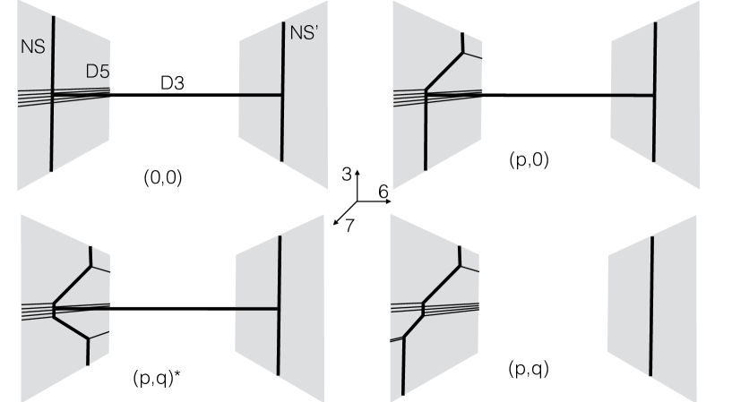
Figure 4: The D3-D5-NS5 brane picture summarizing the dualities of Benini:2011mf . $x_{3}$ is a compact direction.

• Case I: this is Aharony duality. In this case we have the same amount of fundamentals and antifundamentals and giving a real mass is done by moving one semi-infinite D5-branes on the left and on the right of the NS5 brane. In the dual setup the presence of one flavor at $x_{3}=\pi$ is accompanied by the presence of an abelian gauge factor. This is because int he Hanany-Witten transition one D3 brane is created at $x_{3}=\pi$. By locally mirroring such a sector (corresponding to SQED with one flavor) we obtain the electric monopoles acting as singlets in the dual phase, as expected in the Aharony dual theory.

• Case II: this corresponds to assigning a positive (or negative) real mass to some fundamentals (or antifundamentals). Different choices are related by parity transformations. Observe that on the brane setup this corresponds to moving some of the semi-infinite D5-branes along $x_{3}$. In order to preserve supersymmetry this operation requires a motion in the $x_{37}$ plane and the creation of a $(1,k)$-fivebrane. This generates the CS level in the gauge sector. Observe that this motion is not compatible with the effective description on the circle, because the NS5 does not close on itself anymore. Anyway looking at the dual picture we can observe that one of the D1-branes engineering the monopole superpotential survives, and this tells us that we are in presence of half of the original monopole superpotential.

• Case III: the D5’s that have to move are on the same side of the NS5 and two stacks are moved along opposite directions. The CS is the difference in this case and the KK monopole is generically broken, as in case III. This result requires some more care if the number of D5’s going up and down is the same. In this case $k=0$, and in the dual this signals that monopole and antimonopole are integrated out with opposite real mass. The D1 does not survive in the dual case (following the picture this becomes evident).

• Case IV: in this case the flow is generated by moving the left and the right D5-branes in opposite directions. The CS level is additive and both the monopole and the antimonopole are massive in this case.