Curriculum Manager for Source Selection
in Multi-Source Domain Adaptation

Abstract

The performance of Multi-Source Unsupervised Domain Adaptation depends significantly on the effectiveness of transfer from labeled source domain samples. In this paper, we proposed an adversarial agent that learns a dynamic curriculum for source samples, called Curriculum Manager for Source Selection (CMSS). The Curriculum Manager, an independent network module, constantly updates the curriculum during training, and iteratively learns which domains or samples are best suited for aligning to the target. The intuition behind this is to force the Curriculum Manager to constantly re-measure the transferability of latent domains over time to adversarially raise the error rate of the domain discriminator. CMSS does not require any knowledge of the domain labels, yet it outperforms other methods on four well-known benchmarks by significant margins. We also provide interpretable results that shed light on the proposed method.

1 Introduction

Training deep neural networks requires datasets with rich annotations that are often time-consuming to obtain. Previous proposals to mitigate this issue have ranged from unsupervised [21, 18, 42, 29, 8, 30], self-supervised [35, 17, 36, 41], to low shot learning [28, 33, 37, 44]. Unsupervised Domain Adaptation (UDA), when first introduced in [15], sheds precious insights on how adversarial training can be utilized to get around the problem of expensive manual annotations. UDA aims to preserve the performance on an unlabeled dataset (target) using a model trained on a label-rich dataset (source) by making optimal use of the learned representations from the source.

Intuitively, one would expect that having more labeled samples in the source domain will be beneficial. However, having more labeled samples does not equal better transfer, since the source will inadvertently encompass a larger variety of domains. While the goal is to learn a common representation for both source and target in such a Multi-Source Unsupervised Domain Adaptation (MS-UDA) setting, enforcing each source domain distribution to exactly match the target may increase the training difficulty, and generate ambiguous representations near the decision boundary potentially resulting in negative transfer. Moreover, for practical purposes, we would expect the data source to be largely unconstrained, whereby neither the number of domains or domain labels are known. A good example here would be datasets collected from the Internet where images come from unknown but potentially a massive set of users.

To address the MS-UDA problem, we propose an adversarial agent that learns a dynamic curriculum [4] for multiple source domains, named Curriculum Manager for Source Selection (CMSS). More specifically, a constantly updated curriculum during training learns which domains or samples are best suited for aligning to the target distribution. The CMSS is an independent module from the feature network and is trained by maximizing the error of discriminator in order to weigh the gradient reversal back to the feature network. In our proposed adversarial interplay with the discriminator, the Curriculum Manager is forced to constantly re-measure the transferability of latent domains across time to achieve a higher error of the discriminator. Such a procedure of weighing the source data is modulated over the entire training. In effect, the latent domains with different transferability to the target distribution will gradually converge to different levels of importance without any need for additional domain partitioning prior or clustering.

We attribute the following contributions to this work:

• We propose a novel adversarial method during training towards the MS-UDA problem. Our method does not assume any knowledge of the domain labels or the number of domains.

• Our method achieves state-of-the-art in extensive experiments conducted on four well-known benchmarks, including the large-scale DomainNet ($\sim$ 0.6 million images).

• We obtain interpretable results that show how CMSS is in effect a form of curriculum learning that has great effect on MS-UDA when compared to the prior art. This positively differentiates our approach from previous state-of-the-art.

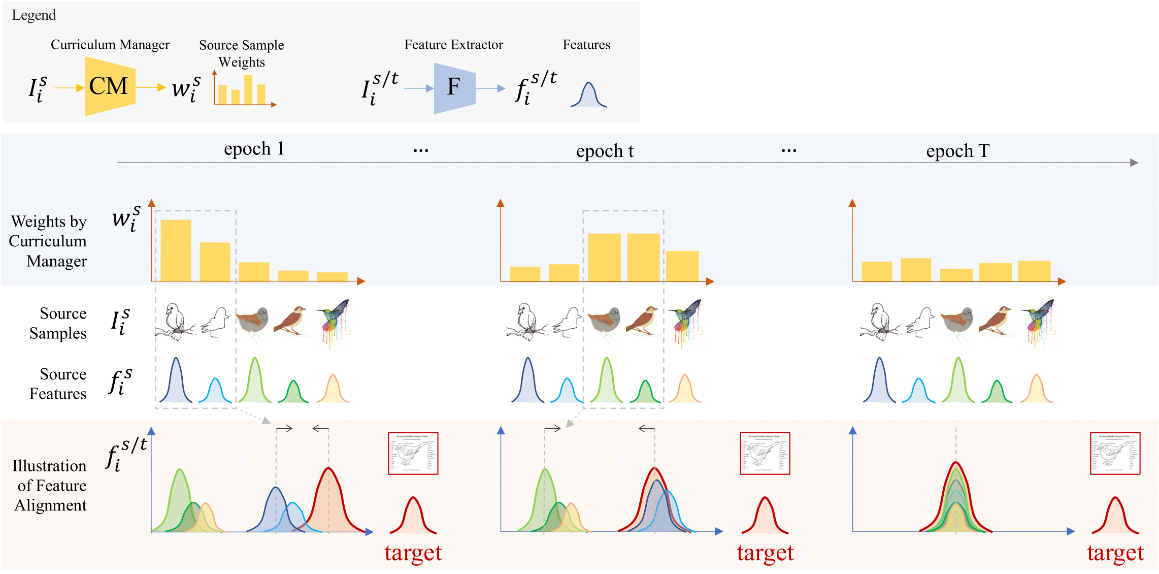
Figure 1: Illustration of CMSS during training. All training samples are passed through the feature network $F$. CMSS prefers samples with better transferability to match the target, and re-measure the transferability at each iteration to keep up with the discriminator. At the end of training after the majority of samples are aligned, the CMSS weights tend to be similar among source samples.

2 Related Work

UDA is an actively studied area of research in machine learning and computer vision. Since the seminal contribution of Ben-David et al. [2, 1], several techniques have been proposed for learning representations invariant to domain shift [23, 11, 25, 10, 45]. In this section, we review some recent methods that are most related to our work.

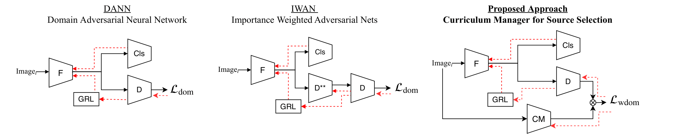
Figure 2: Architecture comparison of left: DANN [15], middle: IWAN [43], and right: proposed method. Red dotted lines indicate backward passes. ($F$: feature extractor, $Cls$: classifier, $D$: domain discriminator, GRL: gradient reversal layer, CM: Curriculum Manager, $\mathcal{L}_{\text{dom}}$: Eq.1 domain loss, $\mathcal{L}_{\text{wdom}}$: Eq.4.0.1 weighted domain loss)

Multi-Source Unsupervised Domain Adaptation (MS-UDA) assumes that the source training examples are inherently multi-modal. The source domains contain labeled samples while the target domain contains unlabeled samples [22, 32, 27, 15, 46]. In [32], adaptation was performed by aligning the moments of feature distributions between each source-target pair. Deep Cocktail Network (DCTN) [40] considered the more realistic case of existence of category shift in addition to the domain shift, and proposes a $k$-way domain adversarial classifier and category classifier to generate a combined representation for the target.

Because domain labels are hard to obtain in the real world datasets, latent domain discovery [27] – a technique for alleviating the need for explicit domain label annotation has many practical applications. Xiong et al. [39] proposed to use square-loss mutual information based clustering with category distribution prior to infer the domain assignment for images. Mancini et al. [27] used a domain prediction branch to guide domain discovery using multiple batch-norm layers.

Domain-Adversarial Training has been widely used [9, 7, 31] since Domain-Adversarial Neural Network (DANN) [15] was proposed. The core idea is to train a discriminator network to discriminate source features from target, and train the feature network to fool the discriminator. Zhao et al. [46] first proposed to generalize DANN to the multi-source setting, and provides theoretical insights on the multi-domain adversarial bounds. Maximum Classifier Discrepancy (MCD) [33] is another powerful [32, 19, 38, 24] technique for performing adaptation in an adversarial manner using two classifiers. The method first updates the classifiers to maximize the discrepancy between the classifiers’ prediction on target samples, followed by minimizing the discrepancy while updating the feature generator.

Domain Selection and Weighting: Some previous methods that employed sample selection and sample weighing techniques for domain adaptation include [13, 14, 12]. Duan et al. [14] proposed using a domain selection machine by leveraging a large number of loosely labeled web images from different sources. The authors of [14] adopted a set of base classifiers to predict labels for the target domain as well as a domain-dependent regularizer based on smoothness assumption. Bhatt et al. [5] proposed to adapt iteratively by selecting the best sources that learn shared representations faster. Chen et al. [9] used a hand-crafted re-weighting vector so that the source domain label distribution is similar to the unknown target label distribution. Mancini et al. [26] modeled the domain dependency using a graph and utilizes auxiliary metadata for predictive domain adaptation. Zhang et al. [43] employed an extra domain classifier that gives the probability of a sample coming from the source domain. The higher the confidence is from such an extra classifier, the more likely it can be discriminated from the target domain, in which case the importance of the said sample is reduced accordingly.

Curriculum for Domain Adaptation aims at an adaptive strategy over time in order to improve the effectiveness of domain transfer. The curriculum can be hand-crafted or learned. Shu et. al [34] designed the curriculum by combining the classification loss and discriminator’s loss as a weighting strategy to eliminate the corrupted samples in the source domain. Another work with similar motivation is [8], in which Chen et. al proposed to use per-category prototype to measure the prediction confidence of target samples. A manually designed threshold $\tau$ is utilized to make a binary decision in selecting partial target samples for further alignment. Kurmi et. al [20] used a curriculum-based dropout discriminator to simulate the gradual increase of sample variance.

3 Preliminaries

3.0.1 Task Formulation:

In multi-source unsupervised domain adaptation (MS-UDA), we are given an input dataset $\mathcal{D}_{\text{src}}=\{(\mathbf{x}_{i}^{s},y_{i}^{s})\}_{i=1}^{N_{s}}$ that contains samples from multiple domains. In this paper, we focus on classification problems, with the set of labels $y_{i}^{s}\in\{1,2,\ldots,n_{c}\}$, where $n_{c}$ is the number of classes. Each sample $\mathbf{x}_{i}^{s}$ has an associated domain label, $d_{i}^{s}\in\{1,2,\ldots,S\}$, where $S$ is the number of source domains. In this work, we assume source domain label information is not known a priori, i.e., number of source domains or source domain label per sample is not known. In addition, given an unlabeled target dataset $\mathcal{D}_{\text{tgt}}=\{\mathbf{x}_{i}^{t}\}_{i=1}^{N_{t}}$, the goal of MS-UDA is to train models using multiple source domains ($\mathcal{D}_{\text{src}}$) and the target domain ($\mathcal{D}_{\text{tgt}}$), and improve performance on the target test set.

3.0.2 Domain-Adversarial training:

First, we discuss the domain-adversarial training formulation from [15] that is the basis from which we extend to MS-UDA. The core idea of domain-adversarial training is to minimize the distributional distance between source and target feature distributions posed as an adversarial game. The model has a feature extractor, a classifier, and a domain discriminator. The classifier takes in feature from the feature extractor and classifies it in $n_{c}$ classes. The discriminator is optimized to discriminate source features from target. The feature network, on the other hand, is trained to fool the discriminator while at the same time achieve good classification accuracy.

More formally, let $F_{\theta}:\mathbb{R}^{3\times w\times h}\to\mathbb{R}^{d}$ denote the feature extraction network, $C_{\phi}:\mathbb{R}^{d}\to\mathbb{R}^{n_{c}}$ denote the classifier, and $D_{\psi}:\mathbb{R}^{d}\to\mathbb{R}^{1}$ denote the domain discriminator. Here, $\theta$, $\phi$ and $\psi$ are the parameters associated with the feature extractor, classifier, and domain discriminator respectively. The model is trained using the following objective function:

$$\max_{\psi}~{}\min_{\theta,\phi}~{}~{}\mathcal{L}_{\text{cls}}-\lambda\mathcal{L}_{\text{dom}}$$ (1)

$$\text{where }~{}~{}~{}~{}\mathcal{L}_{\text{cls}}= -\frac{1}{N_{s}}\sum_{i=1}^{N_{s}}\tilde{\mathbf{y}}_{i}\log(C(F(\mathbf{x}^{s}_{i})))$$

$$\mathcal{L}_{\text{dom}}= -\mathbb{E}_{\mathbf{x}\sim\mathcal{D}_{\text{src}}}\log(D(F(\mathbf{x})))-\mathbb{E}_{\mathbf{x}\sim\mathcal{D}_{\text{tgt}}}\log(1-D(F(\mathbf{x})))$$

$$= -\frac{1}{N_{s}}\sum_{i=1}^{N_{s}}\log(D(F(\mathbf{x}^{s}_{i})))-\frac{1}{N_{t}}\sum_{i=1}^{N_{t}}\log(1-D(F(\mathbf{x}^{t}_{i})))$$

$\mathcal{L}_{\text{cls}}$ is is the cross-entropy loss in source domain (with $\tilde{\mathbf{y}}_{i}$ being the one-hot encoding of the label $y_{i}$), and $\mathcal{L}_{\text{dom}}$ is the discriminator loss that discriminates source samples from the target. Note that both these loss functions use samples from all source domains.

In principle, if domain labels are available, there are two possible choices for the domain discriminator: (1) $k$ domain discriminators can be trained, each one discriminating one of the source domains from the target [15], or (2) a domain discriminator can be trained as a $(k+1)$-way classifier to classify input samples as either one of the source domains or target [46]. However, in our setup, domain labels are unknown and, therefore, these formulations can not be used.

4 CMSS: Curriculum Manager for Source Selection

For the source domain that is inherently multi-modal, our goal is to learn a dynamic curriculum for selecting the best-suited samples for aligning to the target feature distribution. At the beginning of training, the Curriculum Manager is expected to prefer samples with higher transferability for aligning with the target, i.e., source samples which have similar feature distributions to the target sample. Once the feature distributions of these samples are aligned, our Curriculum Manager is expected to prioritize the next round of source samples for alignment. As the training progresses, the Curriculum Manager can learn to focus on different aspects of the feature distribution as a proxy for better transferability. Since our approach learns a curriculum to prefer samples from different source domains, we refer to it is Curriculum Manager for Source Selection (CMSS).

Our approach builds on the domain-adversarial training framework (described in $\S$3). In this framework, our hypothesis is that source samples that are hard for the domain discriminator to separate from the target samples are likely the ones that have similar feature distributions. Our CMSS leverages this and uses the discriminator loss to find source samples that should be aligned first. The preference for source samples is represented as per-sample weights predicted by CMSS. Since our approach is based on domain-adversarial training, weighing $\mathcal{L}_{\text{dom}}$ using these weights will lead to the discriminator encouraging the feature network to bring the distributions of higher weighted source samples closer to the target samples. This signal between the discriminator and feature extractor is achieved using the gradient reversal layer (see [15] for details).

Therefore, our proposed CMSS is trained to predict weights for source samples at each iteration, which maximizes the error of the domain discriminator. Due to this adversarial interplay with the discriminator, the CMSS is forced to re-estimate the preference of source samples across training to keep up with the improving domain discriminator. The feature extractor, $F$, is optimized to learn features that are both good for classification and confuse the discriminator. To avoid any influence from the classification task in the curriculum design, our CMSS also has an independent feature extractor module that learns to predict weights per-sample given the source images and domain discriminator loss.

4.0.1 Training CMSS:

The CMSS weight for every sample in the source domain, $\mathbf{x}^{s}_{i}$, is given by $w^{s}_{i}$. We represent this weighted distribution as $\tilde{\mathcal{D}}_{\text{src}}$. The CMSS network is represented by $G_{\rho}:\mathbb{R}^{c\times w\times h}\to\mathbb{R}^{1}$ with parameters $\rho$. Given a batch of samples, $\mathbf{x}^{s}_{1},\mathbf{x}^{s}_{2},\ldots\mathbf{x}^{s}_{b}$, we first pass these samples to $G_{\rho}$ to obtain an array of scores that are normalized using softmax function to obtain the resulting weight vector. During training, the CMSS optimization objective can be written as

$$\min_{\rho}\left[\frac{1}{N_{s}}\sum_{i=1}^{N_{s}}G_{\rho}(\mathbf{x}^{s}_{i})\log(D(F(\mathbf{x}^{s}_{i})))\right]$$ (2)

With the source sample weights generated by CMSS, the loss function for domain discriminator can be written as

$$\mathcal{L}_{\text{wdom}} =-\frac{1}{N_{s}}\sum_{i=1}^{N_{s}}G_{\rho}(\mathbf{x}^{s}_{i})\log(D(F(\mathbf{x}^{s}_{i})))-\frac{1}{N_{t}}\sum_{i=1}^{N_{t}}\log(1-D(F(\mathbf{x}^{t}_{i})))$$

$$~{}~{}~{}~{}\text{ s.t. }\sum_{i}G_{\rho}(\mathbf{x}^{s}_{i})=N_{s}$$ (3)

The overall optimization objective can be written as

$$\max_{\psi}~{}\min_{\theta,\phi,\rho}~{}~{} \mathcal{L}_{\text{cls}}-\lambda\mathcal{L}_{\text{wdom}}$$ (4)

where $\mathcal{L}_{\text{cls}}$ is the Cross-Entropy loss for source classification and $\mathcal{L}_{\text{wdom}}$ is the weighted domain discriminator loss from Eq. (4.0.1), with weights obtained by optimizing Eq. (2). $\lambda$ is the hyperparameter in the gradient reversal layer. We follow [15] and set $\lambda$ based on the following annealing schedule: $\lambda_{p}=\frac{2}{1+\exp(-\gamma\cdot p)}-1$, where $p$ is the current number of iterations divided by the total. $\gamma$ is set to $10$ in all experiments as in [15]. Details of training are provided in Algorithm  1.

Algorithm 1 Training CMSS (Curriculum Manager for Source Selection)

1:$N_{\text{iter}}$: Total number of training iterations

2:$\gamma$: For computing $\lambda_{p}$ for $\mathcal{L}_{\text{wdom}}$

3:$N_{b}^{s}$ and $N_{b}^{t}$: Batch size for source and target domains

4:Shuffle the source domain samples

5:for $t$ in $(1:N_{\text{iter}})$ do

6:     Compute $\lambda$ according to $2/(1+\exp(-\gamma\cdot(t/N_{iter})))-1$

7:     Sample a training batch from source domains $\{(\mathbf{x}_{i}^{s},y_{i})\}_{i=1}^{N_{b}^{s}}\sim\mathcal{D}_{\text{src}}$ and from target domain $\{\mathbf{x}_{i}^{t}\}_{i=1}^{N_{b}^{t}}\sim\mathcal{D}_{\text{tgt}}$

8:     Update $\rho$ by $\min_{\rho}-\lambda\mathcal{L}_{\text{wdom}}$

9:     Update $\psi$ by $\min_{\psi}\lambda\mathcal{L}_{\text{dom}}$

10:     Update $\theta,\phi$ by $\min_{\theta,\phi}\mathcal{L}_{\text{cls}}-\lambda\mathcal{L}_{\text{wdom}}$

11:end for

4.1 CMSS: Theoretical Insights

We first state the classic generalization bound for domain adaptation [3, 6]. Let $\mathcal{H}$ be a hypothesis space of $VC$-dimension $d$. For a given hypothsis class $\mathcal{H}$, define the symmetric difference operator as $\mathcal{H}\Delta\mathcal{H}=\{h(\mathbf{x})\oplus h^{\prime}(\mathbf{x})|h,h^{\prime}\in\mathcal{H}\}$. Let $\mathcal{D}_{\text{src}}$, $\mathcal{D}_{\text{tgt}}$ denote the source and target distributions respectively, and $\hat{\mathcal{D}}_{\text{src}}$, $\hat{\mathcal{D}}_{\text{tgt}}$ denote the empirical distribution induced by sample of size $m$ drawn from $\mathcal{D}_{\text{src}}$, $\mathcal{D}_{\text{tgt}}$ respectively. Let $\epsilon_{s}$ ($\epsilon_{t}$) denote the true risk on source (target) domain, and $\hat{\epsilon}_{s}$ ($\hat{\epsilon}_{t}$) denote the empirical risk on source (target) domain. Then, following Theorem 1 of [6], with probability of at least $1-\delta$, $\forall h\in\mathcal{H}$ ,

$$\epsilon_{t}(h)\leq\hat{\epsilon}_{s}(h)+\frac{1}{2}d_{\mathcal{H}\Delta\mathcal{H}}(\hat{\mathcal{D}}_{src},\hat{\mathcal{D}}_{tgt})+C$$ (5)

where $C$ is a constant

$$C=\lambda+O\left(\sqrt{\frac{d\log(m/d)+\log(1/\delta)}{m}}\right)$$

Here, $\lambda$ is the optimal combined risk (source + target risk) that can be achieved by hypothesis in $\mathcal{H}$. Let $\{\mathbf{x}^{s}_{i}\}_{i=1}^{m}$, $\{\mathbf{x}^{t}_{i}\}_{i=1}^{m}$ be the samples in the empirical distributions $\hat{\mathcal{D}}_{\text{src}}$ and $\hat{\mathcal{D}}_{\text{tgt}}$ respectively. Then, $P(\mathbf{x}^{s}_{i})=1/m$ and $P(\mathbf{x}^{t}_{i})=1/m$. The empirical source risk can be written as $\hat{\epsilon}_{s}(h)=1/m\sum_{i}\hat{\epsilon}_{\mathbf{x}^{s}_{i}}(h)$

Now consider a CMSS re-weighted source distribution $\hat{\mathcal{D}}_{\text{wsrc}}$, with $P(\mathbf{x}^{s}_{i})=w_{i}$. For $\hat{\mathcal{D}}_{\text{wsrc}}$ to be a valid probability mass function, $\sum_{i}w^{s}_{i}=1$ and $w^{s}_{i}\geq 0$. Note that $\hat{\mathcal{D}}_{\text{src}}$ and $\hat{\mathcal{D}}_{\text{wsrc}}$ share the same samples, and only differ in weights. The generalization bound for this re-weighted distribution can be written as

$$\epsilon_{t}(h)\leq\sum_{i}w_{i}\hat{\epsilon}_{\mathbf{x}^{s}_{i}}(h)+\frac{1}{2}d_{\mathcal{H}\Delta\mathcal{H}}(\hat{\mathcal{D}}_{\text{wsrc}},\hat{\mathcal{D}}_{\text{tgt}})+C$$

Since the bound holds for all weight arrays $\mathbf{w}=[w^{s}_{1},w^{s}_{2}\ldots w^{s}_{m}]$ in a simplex, we can minimize the objective over $\mathbf{w}$ to get a tighter bound.

$$\epsilon_{t}(h)\leq\min_{\mathbf{w}\in\Delta^{m}}\sum_{i}w_{i}\hat{\epsilon}_{\mathbf{x}^{s}_{i}}(h)+\frac{1}{2}d_{\mathcal{H}\Delta\mathcal{H}}(\hat{\mathcal{D}}_{\text{wsrc}},\hat{\mathcal{D}}_{\text{tgt}})+C$$ (6)

The first term is the weighted risk, and the second term $d_{\mathcal{H}\Delta\mathcal{H}}(\hat{\mathcal{D}}_{\text{wsrc}},\hat{\mathcal{D}}_{\text{tgt}})$ is the weighted symmetric divergence which can be realized using our weighted adversarial loss. Note that when $\mathbf{w}=[1/m,1/m,\ldots 1/m]$, we get the original bound (5). Hence, the original bound is in the feasible set of this optimization.

4.1.1 Relaxations.

In practice, deep neural networks are used to optimize the bounds presented above. Since the bound (6) is minimized over the weight vector $\mathbf{w}$, one trivial solution is to assign non-zero weights to only a few source samples. In this case, a neural network can overfit to these source samples, which could result in low training risk and low domain divergence. To avoid this trivial case, we present two relaxations:

• We use the unweighted loss for the source risk (first term in the bound (6)).

• For the divergence term, instead of minimizing $\mathbf{w}$ over all the samples, we optimize only over mini-batches. Hence, for every mini-batch, there is at least one $w_{i}$ which is non-zero. Additionally, we make weights a function of input, i.e., $w_{i}=G_{\rho}(\mathbf{x}^{s}_{i})$, which is realized using a neural network. This will smooth the predictions of $w_{i}$, and make the weight network produce a soft-selection over source samples based on correlation with the target.

Note that the $G_{\rho}$ network discussed in the previous section satisfies these criteria.

5 Experimental Results

In this section, we perform an extensive evaluation of the proposed method on the following tasks: digit classification(MNIST, MNIST-M, SVHN, Synthetic Digits, USPS), image recognition on the large-scale DomainNet dataset (clipart, infograph, paiting, quickdraw, real, sketch), PACS[22] (art, cartoon, photo and sketch) and Office-Caltech10 (Amazon, Caltech, Dslr, Webcam). We compare our method with the following contemporary approaches: Domain Adversarial Neural Network (DANN) [15], Multi-Domain Adversarial Neural Network (MDAN)[46] and two state-of-the-art discrepancy-based approaches: Maximum Classifier Discrepancy (MCD) [33] and Moment Matching for Multi-Source ($M^{3}$SDA) [32]. We follow the protocol used in other multi-source domain adaptation works [27, 32], where each domain is selected as the target domain while the rest of domains are used as source domains. For Source Only and DANN experiments, all source domains are shuffled and treated as one domain. To guarantee fairness of comparison, we used the same model architectures, batch size and data pre-processing routines for all compared approaches. All our experiments are implemented in PyTorch.

5.1 Experiments on Digit Recognition

Following DCTN [40] and $M^{3}$SDA [32], we sample $25000$ images from training subset and $9000$ from testing subset of MNIST, MNIST-M, SVHN and Synthetic Digits. The entire USPS is used since it contains only $9298$ images in total.

In all the experiments, the feature extractor is composed of three $conv$ layers and two $fc$ layers. The entire network is trained from scratch with batch size equals $16$. For each experiment, we run the same setting five times and report the mean and standard deviation. (See Appendix for more experiment details and analyses.) The results are shown in Table 1. The proposed method achieves an 90.8% average accuracy, outperforming other baselines by a large margin ($\sim 3\%$ improvement on the previous state-of-the-art approach).

Table 1: Results on Digits classification. The proposed CMSS achieves 90.8% accuracy. Comparisons with MCD and $M^{3}SDA$ are reprinted from [32]. All experiments are based on a 3-$conv$-layer backbone trained from scratch. (mt, mm, sv, sy, up: MNIST, MNIST-M, SVHN, Synthetic Digits, UPSP)

Models	$mm,sv,sy,up$	$mt,sv,sy,up$	$mt,mm,sy,up$	$mt,mm,sv,up$	$mt,mm,sv,sy$	Avg
	$\to$ $mt$	$\to$ $mm$	$\to$ $sv$	$\to$ $sy$	$\to$ $up$
Source Only	92.3 $\pm$ 0.91	63.7 $\pm$ 0.83	71.5 $\pm$ 0.75	83.4 $\pm$ 0.79	90.7 $\pm$ 0.54	80.3 $\pm$ 0.76
DANN[15]	97.9 $\pm$ 0.83	70.8 $\pm$ 0.94	68.5 $\pm$ 0.85	87.3 $\pm$ 0.68	93.4 $\pm$ 0.79	83.6 $\pm$ 0.82
MDAN[46]	97.2 $\pm$ 0.98	75.7 $\pm$ 0.83	82.2 $\pm$ 0.82	85.2 $\pm$ 0.58	93.3 $\pm$ 0.48	86.7 $\pm$ 0.74
MCD[33]	96.2 $\pm$ 0.81	72.5 $\pm$ 0.67	78.8 $\pm$ 0.78	87.4 $\pm$ 0.65	95.3 $\pm$ 0.74	86.1 $\pm$ 0.64
$M^{3}$SDA[32]	98.4 $\pm$ 0.68	72.8 $\pm$ 1.13	81.3 $\pm$ 0.86	89.5 $\pm$ 0.56	96.1 $\pm$ 0.81	87.6 $\pm$ 0.75
CMSS	99.0 $\pm$ 0.08	75.3 $\pm$ 0.57	88.4 $\pm$ 0.54	93.7 $\pm$ 0.21	97.7 $\pm$ 0.13	90.8 $\pm$ 0.31

5.2 Experiments on DomainNet

Next, we evaluate our method on DomainNet [32] – a large-scale benchmark dataset used for multi-domain adaptation. The DomainNet dataset contains samples from $6$ domains: Clipart, Infograph, Painting, Quickdraw, Real and Sketch. Each domain has 345 categories, and the dataset has $\sim$ 0.6 million images in total, which is the largest existing domain adaptation dataset. We use ResNet-101 pretrained on ImageNet as the feature extractor for in all our experiments. For CMSS, we use a ResNet-18 pretrained on ImageNet. The batch size is fixed to $128$. We conduct experiments over $5$ random runs, and report mean and standard deviation over the 5 runs.

The results are shown in Table 2. CMSS achieves 46.5% average accuracy, outperforming other baselines by a large margin. We also note that our approach achieves the best performance in each experimental setting. It is also worth mentioning that in the experiment when the target domain is Quickdraw (q), our approach is the only one that outperforms Source Only baseline, while all other compared approaches result in negative transfer (lower performance than the source-only model). This is since quickdraw has a significant domain shift compared to all other domains. This shows that our approach can effectively alleviate negative transfer even in such challenging set-up.

Table 2: Results on the DomainNet dataset. CMSS achieves $46.5\%$ average accuracy. When the target domain is quickdraw ${\color[rgb]{0,0,1}q}$, CMSS is the only one that outperforms Source Only which indicates negative transfer has been alleviated. Source Only * is re-printed from [32], Source Only is our implemented results. All experiments are based on ResNet-101 pre-trained on ImageNet. ($c$: clipart, $i$: infograph, $p$: painting, $q$: quickdraw, $r$: real, $s$: sketch)

Models	$i,p,q$	$c,p,q$	$c,i,q$	$c,i,p$	$c,i,p$	$c,i,p$	Avg
	$r,s$ $\to$ $c$	$r,s$ $\to$ $i$	$r,s$ $\to$ $p$	$r,s$ $\to$ $q$	$q,s$ $\to$ $r$	$q,r$ $\to$ $s$
Source Only*	47.6$\pm$0.52	13.0$\pm$0.41	38.1$\pm$0.45	13.3$\pm$0.39	51.9$\pm$0.85	33.7$\pm$0.54	32.9$\pm$0.54
Source Only	52.1$\pm$0.51	23.4$\pm$0.28	47.7$\pm$0.96	13.0$\pm$0.72	60.7$\pm$0.32	46.5$\pm$0.56	40.6$\pm$0.56
DANN[15]	60.6$\pm$0.42	25.8$\pm$0.34	50.4$\pm$0.51	7.7$\pm$0.68	62.0$\pm$0.66	51.7$\pm$0.19	43.0$\pm$0.46
MDAN[46]	60.3$\pm$0.41	25.0$\pm$0.43	50.3$\pm$0.36	8.2$\pm$1.92	61.5$\pm$0.46	51.3$\pm$0.58	42.8$\pm$0.69
MCD[33]	54.3$\pm$0.64	22.1$\pm$0.70	45.7$\pm$0.63	7.6$\pm$0.49	58.4$\pm$0.65	43.5$\pm$0.57	38.5$\pm$0.61
$M^{3}$SDA[32]	58.6$\pm$0.53	26.0$\pm$0.89	52.3$\pm$0.55	6.3$\pm$0.58	62.7$\pm$0.51	49.5$\pm$0.76	42.6$\pm$0.64
CMSS	64.2$\pm$0.18	28.0$\pm$0.20	53.6$\pm$0.39	16.0$\pm$0.12	63.4$\pm$0.21	53.8$\pm$0.35	46.5$\pm$0.24

5.3 Experiments on PACS

PACS [22] is another popular benchmark for multi-source domain adaptation. It contains 4 domains: art, cartoon, photo and sketch. Images of 7 categories are collected for each domain. There are $9991$ images in total. For all experiments, we used ResNet-18 pretrained on ImageNet as the feature extractor following [27]. For the Curriculum Manager, we use the same architecture as the feature extractor. Batch size of $32$ is used. We conduct experiments over $5$ random runs, and report mean and standard deviation over the runs. The results are shown in Table 4 ($a$: art, $c$: cartoon, $p$: painting, $s$: sketch.). CMSS achieves the state-of-the-art average accuracy of 89.5%. On the most challenging sketch (s) domain, we obtain 82.0%, outperforming other baselines by a large margin.

Table 3: Results on PACS

Models	$c,p,s$ $\to$ $a$	$a,p,s$ $\to$ $c$	$a,c,s$ $\to$ $p$	$a,c,p$ $\to$ $s$	Avg
Source Only	74.9$\pm$0.88	72.1$\pm$0.75	94.5$\pm$0.58	64.7$\pm$1.53	76.6$\pm$0.93
DANN[15]	81.9$\pm$1.13	77.5$\pm$1.26	91.8$\pm$1.21	74.6$\pm$1.03	81.5$\pm$1.16
MDAN[46]	79.1$\pm$0.36	76.0$\pm$0.73	91.4$\pm$0.85	72.0$\pm$0.80	79.6$\pm$0.69
WBN[27]	89.9$\pm$0.28	89.7$\pm$0.56	97.4$\pm$0.84	58.0$\pm$1.51	83.8$\pm$0.80
MCD[33]	88.7$\pm$1.01	88.9$\pm$1.53	96.4$\pm$0.42	73.9$\pm$3.94	87.0$\pm$1.73
$M^{3}$SDA[32]	89.3$\pm$0.42	89.9$\pm$1.00	97.3$\pm$0.31	76.7$\pm$2.86	88.3$\pm$1.15
CMSS	88.6$\pm$0.36	90.4$\pm$0.80	96.9$\pm$0.27	82.0$\pm$0.59	89.5$\pm$0.50

Table 4: Results on Office-Caltech10

Models	$A,C,D$	$A,C,W$	$A,D,W$	$C,D,W$	Avg
	$\to$ $W$	$\to$ $D$	$\to$ $C$	$\to$ $A$
Source Only	99.0	98.3	87.8	86.1	92.8
DANN[15]	99.3	98.2	89.7	94.8	95.5
MDAN[46]	98.9	98.6	91.8	95.4	96.1
MCD[33]	99.5	99.1	91.5	92.1	95.6
$M^{3}$SDA[32]	99.5	99.2	92.2	94.5	96.4
CMSS	99.6	99.3	93.7	96.0	97.2

5.4 Experiments on Office-Caltech10

The office-Caltech10 [16] dataset has 10 object categories from 4 different domains: Amazon, Caltech, DSLR, and Webcam. For all the experiments, we use the same architecture (ResNet-101 pretrained on ImageNet) used in [32]. The experimental results are shown in Table 4 (A: Amazon, C: Caltech, D: Dslr, W: Webcam). CMSS achieves state-of-the-art average accuracy of 97.2$\%$.

5.5 Comparison with other re-weighting methods

In this experiment, we compare CMSS with other weighing schemes proposed in the literature. We use IWAN [43] for this purpose. IWAN, originally proposed for partial domain adaption, reweights the samples in adversarial training using outputs of discriminator as sample weights (Refer to Figure 2). CMSS, however, computes sample weights using a separate network $G_{\rho}$ updated using an adversarial game. We adapt IWAN for multi-source setup and compare it against our approach. The results are shown in Table 5 (abbreviations of domains same as Table 2). IWAN obtained $43.1\%$ average accuracy which is close to performance obtained using DANN with combined source domains. For further analysis, we plot how sample weights estimated by both approaches (plotted as mean $\pm$ variance) change as training progresses in Figure 3. We observe that CMSS selects weights with larger variance which demonstrates its sample selection ability, while IWAN has weights all close to $1$ (in which case, it becomes similar to DANN). This illustrates the superiority of our sample selection method. More discussions on sample selection can be found in Section 6.2. CMSS also achieves a faster and more stable convergence in test accuracy compared to DANN [15] where we assume a single source domain (Figure 6), which further supports the effectiveness of the learnt curriculum.

Table 5: Comparing re-weighting methods

Models	$i,p,q$	$c,p,q$	$c,i,q$	$c,i,p$	$c,i,p$	$c,i,p$	Avg
	$r,s$ $\to$ $c$	$r,s$ $\to$ $i$	$r,s$ $\to$ $p$	$r,s$ $\to$ $q$	$q,s$ $\to$ $r$	$q,r$ $\to$ $s$
DANN[15]	60.6	25.8	50.4	7.7	62.0	51.7	43.0
IWAN[43]	59.1	25.2	49.7	12.9	60.4	51.4	43.1
CMSS	64.2	28.0	53.6	16.0	63.4	53.8	46.5

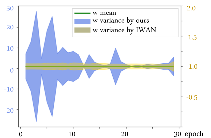
Figure 3: Mean/var of weights over time.

Figure 4: Interpretation results of the sample selection on DomainNet dataset using the proposed method. In each plot, one domain is selected as the target. In each setting, predictions of CMSS are computed for each sample of the source domains. The bars indicate how many of these samples have weight prediction larger than a manually chosen threshold, with each bar denoting a single source domain. Maximum number of samples are highlighted in red. Best viewed in color

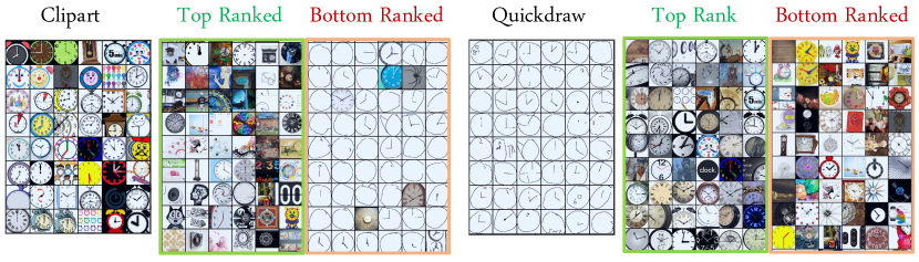
Figure 5: Ranked source samples according to learnt weights (class “Clock” of DomainNet dataset). LHS: Examples of unlabeled target domain Clipart and the Top/Bottom Ranked $\sim$ 50 samples of the source domain composed of Infograph, Painting, Quickdraw, Real and Sketch. RHS: Examples of unlabeled target domain Quickdraw and the Ranked samples of source domain composed of Clipart, Infograph, Painting, Real and Sketch. Weights are obtained at inference time using CMSS trained after $5$ epochs.

6 Interpretations

In this section, we are interested in understanding and visualizing the source selection ability of our approach. We conduct two sets of experiments: (i) visualizations of the source selection curriculum over time, and (ii) comparison of our selection mechanism with other sample re-weighting methods.

6.1 Visualizations of source selection

6.1.1 Domain Preference

We first investigate if CMSS indeed exhibits domain preference over the course of training as claimed. For this experiment, we randomly select $m=34000$ training samples from each source domain in DomainNet and obtain the raw weights (before softmax) generated by CMSS. Then, we calculate the number of samples in each domain passing a manually selected threshold $\tau$. We use the number of samples passing this threshold in each domain to indicate the domain preference level. The larger the fraction, more weights are given to samples from the domains, hence, higher the domain preference. Figure 4 shows the visualization of domain preference for each target domain. We picked $3$ different $\tau$ in each experiment for more precise observation. We observe that CMSS does display domain preference (Clipart - Painting, Infograph - Sketch, Real - Clipart) that is in fact correlated with the visual similarity of the domains. An exception is Quickdraw, where no domain preference is observed. We argue that this is because Quickdraw has significant domain shift compared to all other domains, hence no specific domain is preferred. However, CMSS still produces better performance on Quickdraw. While there is no domain preference for Quickdraw, there is within-domain sample preference as illustrated in Figure 5. That is, our approach chooses samples within a domain that are structurally more similar to the target domain of interest. Hence, just visualizing aggregate domain preference does not depict the complete picture. We will present sample-wise visualization in the next section.

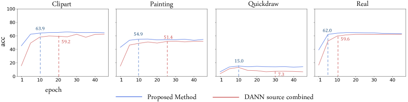
Figure 6: Test accuracy after the model is trained for $t$ epochs. Comparison between CMSS and DANN using source domains combined as one.

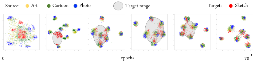
Figure 7: t-SNE visualization of features at six different epochs during training. The shaded region is the migrated range of target features. Dateset used is PACS with sketch as the target domain.

6.1.2 Beyond Domain Preference

In addition to domain preference, we are interested in taking a closer look at sample-wise source selection. To do this, we first obtain the weights generated by CMSS for all source samples and rank the source images according to their weights. An example is shown in Figure 5. For better understanding, we visualize samples belonging to a fixed category (“Clock” in Figure 5). See Appendix for more visualizations.

In Figure 5, we find that notion of similarity discovered by CMSS is different for different domains. When the target domain is Clipart (left panel of Figure 5), source samples with colors and cartoonish shapes are ranked at the top, while samples with white background and simplistic shapes are ranked at the bottom. When the target is Quickdraw (right panel of Figure 5), one would think that CMSS will simply be selecting images with similar white background. Instead, it prefers samples which are structurally similar to the regular rounded clock shape (as most samples in Quickdraw are similar to these). It thus appears that structural similarity is favored in Quickdraw, whereas color information is preferred in Clipart. This provides support that CMSS selects samples according to ease of alignment to the target distribution, which is automatically discovered per domain. We argue that this property of CMSS has an advantage over approaches such as MDAN [46] which simply weighs manually partitioned domains.

6.2 Selection Over Time

In this section, we discuss how source selection varies as training progresses. In Figure 3, we plot mean and variance of weights (output of Curriculum Manager) over training iterations. We observe that the variance is high initially, which indicates many samples have weights away from the mean value of $1$. Samples with higher weights are preferred, while those with low weights contribute less to the alignment. In the later stages, the variance is very low which indicates most of the weights are close to $1$. Hence, our approach gradually adapts to increasingly many source samples over time, naturally learning a curriculum for adaptation. In Figure 7, we plot a t-SNE visualization of features at different epochs. We observe that the target domain sketch (red) first adapts to Art (yellow), and then gradually aligns with Cartoon (green) and Photo (blue).

7 Conclusion

In this paper, we proposed Curriculum Manager for Source Selection (CMSS) that learns a curriculum for Multi-Source Unsupervised Domain Adaptation. A curriculum is learnt that iteratively favors source samples that align better with the target distribution over the entire training. The curriculum learning is achieved by an adversarial interplay with the discriminator, and achieves state-of-the-art on four benchmark datasets. We also shed light on the inner workings of CMSS, and we hope that will pave the way for further advances to be made in this research area.

References

- [1] Ben-David, S., Blitzer, J., Crammer, K., Kulesza, A., Pereira, F., Vaughan, J.W.: A theory of learning from different domains. Machine learning 79(1-2), 151–175 (2010)
- [2] Ben-David, S., Blitzer, J., Crammer, K., Pereira, F.: Analysis of representations for domain adaptation. In: Advances in neural information processing systems. pp. 137–144 (2007)
- [3] Ben-David, S., Blitzer, J., Crammer, K., Pereira, F.: Analysis of representations for domain adaptation. In: Schölkopf, B., Platt, J.C., Hoffman, T. (eds.) Advances in Neural Information Processing Systems 19, pp. 137–144. MIT Press (2007)
- [4] Bengio, Y., Louradour, J., Collobert, R., Weston, J.: Curriculum learning. In: Proceedings of the 26th Annual International Conference on Machine Learning. p. 41–48. ICML ’09, Association for Computing Machinery, New York, NY, USA (2009)
- [5] Bhatt, H.S., Rajkumar, A., Roy, S.: Multi-source iterative adaptation for cross-domain classification. In: IJCAI. pp. 3691–3697 (2016)
- [6] Blitzer, J., Crammer, K., Kulesza, A., Pereira, F., Wortman, J.: Learning bounds for domain adaptation. In: Platt, J.C., Koller, D., Singer, Y., Roweis, S.T. (eds.) Advances in Neural Information Processing Systems 20, pp. 129–136. Curran Associates, Inc. (2008)
- [7] Cao, Z., Long, M., Wang, J., Jordan, M.I.: Partial transfer learning with selective adversarial networks. In: Proceedings of the IEEE Conference on Computer Vision and Pattern Recognition. pp. 2724–2732 (2018)
- [8] Chen, C., Xie, W., Huang, W., Rong, Y., Ding, X., Huang, Y., Xu, T., Huang, J.: Progressive feature alignment for unsupervised domain adaptation. In: Proceedings of the IEEE Conference on Computer Vision and Pattern Recognition. pp. 627–636 (2019)
- [9] Chen, Q., Liu, Y., Wang, Z., Wassell, I., Chetty, K.: Re-weighted adversarial adaptation network for unsupervised domain adaptation. In: Proceedings of the IEEE Conference on Computer Vision and Pattern Recognition. pp. 7976–7985 (2018)
- [10] Chen, Y., Li, W., Sakaridis, C., Dai, D., Van Gool, L.: Domain adaptive faster r-cnn for object detection in the wild. In: Proceedings of the IEEE conference on computer vision and pattern recognition. pp. 3339–3348 (2018)
- [11] Ding, Z., Nasrabadi, N.M., Fu, Y.: Semi-supervised deep domain adaptation via coupled neural networks. IEEE Transactions on Image Processing 27(11), 5214–5224 (2018)
- [12] Duan, L., Tsang, I.W., Xu, D., Chua, T.S.: Domain adaptation from multiple sources via auxiliary classifiers. In: Proceedings of the 26th Annual International Conference on Machine Learning. pp. 289–296. ACM (2009)
- [13] Duan, L., Xu, D., Chang, S.F.: Exploiting web images for event recognition in consumer videos: A multiple source domain adaptation approach. In: 2012 IEEE Conference on Computer Vision and Pattern Recognition. pp. 1338–1345. IEEE (2012)
- [14] Duan, L., Xu, D., Tsang, I.W.H.: Domain adaptation from multiple sources: A domain-dependent regularization approach. IEEE Transactions on Neural Networks and Learning Systems 23(3), 504–518 (2012)
- [15] Ganin, Y., Lempitsky, V.: Unsupervised domain adaptation by backpropagation. arXiv preprint arXiv:1409.7495 (2014)
- [16] Gong, B., Shi, Y., Sha, F., Grauman, K.: Geodesic flow kernel for unsupervised domain adaptation. In: 2012 IEEE Conference on Computer Vision and Pattern Recognition. pp. 2066–2073. IEEE (2012)
- [17] Jeong, R., Aytar, Y., Khosid, D., Zhou, Y., Kay, J., Lampe, T., Bousmalis, K., Nori, F.: Self-supervised sim-to-real adaptation for visual robotic manipulation. arXiv preprint arXiv:1910.09470 (2019)
- [18] Kang, G., Jiang, L., Yang, Y., Hauptmann, A.G.: Contrastive adaptation network for unsupervised domain adaptation. In: Proceedings of the IEEE Conference on Computer Vision and Pattern Recognition. pp. 4893–4902 (2019)
- [19] Kumar, A., Sattigeri, P., Wadhawan, K., Karlinsky, L., Feris, R., Freeman, B., Wornell, G.: Co-regularized alignment for unsupervised domain adaptation. In: Advances in Neural Information Processing Systems. pp. 9345–9356 (2018)
- [20] Kurmi, V.K., Bajaj, V., Subramanian, V.K., Namboodiri, V.P.: Curriculum based dropout discriminator for domain adaptation. arXiv preprint arXiv:1907.10628 (2019)
- [21] Lee, S., Kim, D., Kim, N., Jeong, S.G.: Drop to adapt: Learning discriminative features for unsupervised domain adaptation. In: Proceedings of the IEEE International Conference on Computer Vision. pp. 91–100 (2019)
- [22] Li, D., Yang, Y., Song, Y.Z., Hospedales, T.M.: Deeper, broader and artier domain generalization. In: Proceedings of the IEEE International Conference on Computer Vision. pp. 5542–5550 (2017)
- [23] Li, Y., Tian, X., Gong, M., Liu, Y., Liu, T., Zhang, K., Tao, D.: Deep domain generalization via conditional invariant adversarial networks. In: Proceedings of the European Conference on Computer Vision. pp. 624–639 (2018)
- [24] Liu, H., Long, M., Wang, J., Jordan, M.: Transferable adversarial training: A general approach to adapting deep classifiers. In: International Conference on Machine Learning. pp. 4013–4022 (2019)
- [25] Luo, Y., Zheng, L., Guan, T., Yu, J., Yang, Y.: Taking a closer look at domain shift: Category-level adversaries for semantics consistent domain adaptation. In: Proceedings of the IEEE Conference on Computer Vision and Pattern Recognition. pp. 2507–2516 (2019)
- [26] Mancini, M., Bulò, S.R., Caputo, B., Ricci, E.: Adagraph: Unifying predictive and continuous domain adaptation through graphs. In: Proceedings of the IEEE Conference on Computer Vision and Pattern Recognition. pp. 6568–6577 (2019)
- [27] Mancini, M., Porzi, L., Rota Bulò, S., Caputo, B., Ricci, E.: Boosting domain adaptation by discovering latent domains. In: Proceedings of the IEEE Conference on Computer Vision and Pattern Recognition. pp. 3771–3780 (2018)
- [28] Motiian, S., Jones, Q., Iranmanesh, S., Doretto, G.: Few-shot adversarial domain adaptation. In: Advances in Neural Information Processing Systems. pp. 6670–6680 (2017)
- [29] Ouyang, C., Kamnitsas, K., Biffi, C., Duan, J., Rueckert, D.: Data efficient unsupervised domain adaptation for cross-modality image segmentation. In: International Conference on Medical Image Computing and Computer-Assisted Intervention. pp. 669–677. Springer (2019)
- [30] Pan, Y., Yao, T., Li, Y., Wang, Y., Ngo, C.W., Mei, T.: Transferrable prototypical networks for unsupervised domain adaptation. In: Proceedings of the IEEE Conference on Computer Vision and Pattern Recognition. pp. 2239–2247 (2019)
- [31] Pei, Z., Cao, Z., Long, M., Wang, J.: Multi-adversarial domain adaptation. In: Thirty-Second AAAI Conference on Artificial Intelligence (2018)
- [32] Peng, X., Bai, Q., Xia, X., Huang, Z., Saenko, K., Wang, B.: Moment matching for multi-source domain adaptation. arXiv preprint arXiv:1812.01754 (2018)
- [33] Saito, K., Watanabe, K., Ushiku, Y., Harada, T.: Maximum classifier discrepancy for unsupervised domain adaptation. In: Proceedings of the IEEE Conference on Computer Vision and Pattern Recognition. pp. 3723–3732 (2018)
- [34] Shu, Y., Cao, Z., Long, M., Wang, J.: Transferable curriculum for weakly-supervised domain adaptation. In: Proceedings of the AAAI Conference on Artificial Intelligence. vol. 33, pp. 4951–4958 (2019)
- [35] Sun, Y., Tzeng, E., Darrell, T., Efros, A.A.: Unsupervised domain adaptation through self-supervision. arXiv preprint arXiv:1909.11825 (2019)
- [36] Valada, A., Mohan, R., Burgard, W.: Self-supervised model adaptation for multimodal semantic segmentation. International Journal of Computer Vision pp. 1–47 (2019)
- [37] Wang, T., Zhang, X., Yuan, L., Feng, J.: Few-shot adaptive faster r-cnn. In: Proceedings of the IEEE Conference on Computer Vision and Pattern Recognition. pp. 7173–7182 (2019)
- [38] Wu, Z., Wang, X., Gonzalez, J.E., Goldstein, T., Davis, L.S.: Ace: Adapting to changing environments for semantic segmentation. arXiv preprint arXiv:1904.06268 (2019)
- [39] Xiong, C., McCloskey, S., Hsieh, S.H., Corso, J.J.: Latent domains modeling for visual domain adaptation. In: Twenty-Eighth AAAI Conference on Artificial Intelligence (2014)
- [40] Xu, R., Chen, Z., Zuo, W., Yan, J., Lin, L.: Deep cocktail network: Multi-source unsupervised domain adaptation with category shift. In: Proceedings of the IEEE Conference on Computer Vision and Pattern Recognition. pp. 3964–3973 (2018)
- [41] Yoon, J.S., Shiratori, T., Yu, S.I., Park, H.S.: Self-supervised adaptation of high-fidelity face models for monocular performance tracking. In: Proceedings of the IEEE Conference on Computer Vision and Pattern Recognition. pp. 4601–4609 (2019)
- [42] You, K., Wang, X., Long, M., Jordan, M.: Towards accurate model selection in deep unsupervised domain adaptation. In: International Conference on Machine Learning. pp. 7124–7133 (2019)
- [43] Zhang, J., Ding, Z., Li, W., Ogunbona, P.: Importance weighted adversarial nets for partial domain adaptation. In: Proceedings of the IEEE Conference on Computer Vision and Pattern Recognition. pp. 8156–8164 (2018)
- [44] Zhang, J., Chen, Z., Huang, J., Lin, L., Zhang, D.: Few-shot structured domain adaptation for virtual-to-real scene parsing. In: Proceedings of the IEEE International Conference on Computer Vision Workshops. pp. 0–0 (2019)
- [45] Zhao, H., Combes, R.T.d., Zhang, K., Gordon, G.J.: On learning invariant representation for domain adaptation. arXiv preprint arXiv:1901.09453 (2019)
- [46] Zhao, H., Zhang, S., Wu, G., Moura, J.M., Costeira, J.P., Gordon, G.J.: Adversarial multiple source domain adaptation. In: Advances in Neural Information Processing Systems. pp. 8559–8570 (2018)