Testing the accuracy of 3D-HST photometric redshift estimates as reference samples for deep weak lensing studies

Abstract

Accurate weak lensing mass estimates of clusters are needed in order to calibrate mass proxies for the cosmological exploitation of galaxy cluster surveys. Such measurements require accurate knowledge of the redshift distribution of the weak lensing source galaxies. In this context, we investigate the accuracy of photometric redshifts (photo-$z$s) computed by the 3D-HST team for the Cosmic Assembly Near-infrared Deep Extragalactic Legacy Survey fields, which provide a relevant photometric reference data set for deep weak lensing studies. Through the comparison to spectroscopic redshifts and photo-$z$s based on very deep data from the Hubble Ultra Deep Field, we identify catastrophic redshift outliers in the 3D-HST/CANDELS catalogue. These would significantly bias weak lensing results if not accounted for. We investigate the cause of these outliers and demonstrate that the interpolation of spectral energy distribution (SED) templates and a well-selected combination of photometric data can reduce the net impact for weak lensing studies.

1 Introduction

Weak gravitational lensing is widely known as a tool to study the large-scale structure of the Universe. Distortions of light caused by massive objects within the cosmic web can be used to obtain unbiased estimates of the mass of these objects. One approach to constrain cosmology via weak lensing measurements is provided by cosmic shear (e.g. Schrabback et al., 2010; Jee et al., 2016; Hildebrandt et al., 2018; Troxel et al., 2018; van Uitert et al., 2018; Hikage et al., 2019; Chang et al., 2019). Another route where weak lensing measurements aid cosmological investigations are cluster number counts experiments (e.g. Reiprich & Böhringer, 2002; Allen et al., 2011). In order to infer cosmological constraints from cluster surveys (e.g. Rozo et al., 2010; Mantz et al., 2014; Schellenberger & Reiprich, 2017; Bocquet et al., 2019), we need to calibrate mass-observable scaling relations using weak lensing measurements over a broad redshift range. Galaxy cluster weak lensing mass calibration has so far mostly been done using ground-based data for low redshift clusters (e.g. Marrone et al., 2012; von der Linden et al., 2014; Hoekstra et al., 2015; Applegate et al., 2016; Okabe & Smith, 2016; Stern et al., 2019; Dietrich et al., 2019; McClintock et al., 2019) and space-based data studies of high redshift clusters (e.g. Leauthaud et al., 2010; Hoekstra et al., 2011; Jee et al., 2011; Schrabback et al., 2018).

The South Pole Telescope Sunyaev-Zel’dovich (SPT-SZ) survey (Bleem et al., 2015) has detected a large of sample massive clusters via their Sunyaev-Zel’dovich (SZ; Sunyaev & Zeldovich, 1970, 1972) signal that extend out to high redshifts. Schrabback et al. (2018, S18 hereafter) have performed a weak lensing analysis of a total of 13 high-redshift ($z_{\mathrm{median}}=0.88$) SPT-SZ galaxy clusters in order to aid the SPT-SZ cluster cosmology analysis (Bocquet et al., 2019).

To achieve accurate mass measurements from weak lensing, rigorous measurements of the shapes and redshift distributions of the weak lensing source galaxies must be obtained. The strength of weak lensing signals scales with the redshift-dependent geometric lensing efficiency. In order to accurately interpret the lensing signal and constrain mass models, accurate estimates of the source redshift distribution are therefore indispensable. Due to incompleteness at faint magnitudes, spectroscopic redshifts (spec-$z$s) of galaxies are typically insufficient to fully describe the redshift distribution for faint source samples. If there is sufficient photometric data, photometric redshifts (photo-$z$s) can be estimated directly from the weak lensing survey (e.g. de Jong et al., 2013; Hildebrandt et al., 2017). To probe the weak lensing signal of high-redshift lenses, deeper data are needed, making it expensive to obtain observations in many bands for a large number of targets. A more cost-effective strategy is to obtain cluster field imaging in a few photometric bands only, which are chosen depending on the cluster redshift to facilitate an efficient selection of the main background source population via colour-cuts. A consistent colour selection must then be applied to photometric data from well-studied reference fields that had been covered over a wide range in wavelength, thus providing sufficient amount of photometric data to achieve reliable photo-$z$s (Benítez et al., 2009). In both cases a careful calibration of the inferred redshift distribution is required. This may employ deep spec-$z$s (e.g. Hildebrandt et al., 2018) and potentially higher quality photo-$z$s (e.g. Tanaka et al., 2018).

S18 employed data from the Cosmic Assembly Near-infrared Deep Extragalactic Legacy Survey (CANDELS; Koekemoer et al., 2011; Grogin et al., 2011; Galametz et al., 2013) in order to calibrate the redshift distribution. Importantly, CANDELS includes deep $Hubble\ Space\ Telescope$ ($HST$) near-infrared (NIR) imaging, which greatly improves the photometric redshift estimation of $z\sim 2$ galaxies by probing their $4000\textup{\AA}$/Balmer break. CANDELS also provides sufficient sky coverage over five lines of sight to suppress the impact of line-of-sight variations. Most of the CANDELS fields are also covered by the $HST$ $F814W$ and $F606W$ bands as needed for the colour selection that is used by S18 to remove cluster galaxies and reduce foreground contamination.

In particular S18 employed CANDELS photo-$z$s from 3D-HST (Skelton et al., 2014, S14 hereafter) as reference sample. S18 investigated the photo-$z$ accuracy through comparisons with the Hubble Ultra Deep Field (HUDF; Beckwith et al., 2006) data. They found significant issues with redshift outliers, for which they introduce an approximate empirical re-calibration scheme. The fact that this correction leads to a large ($12\%$) mass bias correction motivates further in-depth analysis of this important systematic issue, which is presented in this paper.

In Section 2 we describe the data and catalogues that are used for our calibrations and tests. In Section 3, we give a summary of the work done by S18, and describe the galaxy selection criteria that are relevant for this work. Section 4 details the comparison metric and the employed photo-$z$ codes. In Section 5, we present our main analysis and results, based on the comparison of different redshift samples, including various sets of photo-$z$s that are computed based on the 3D-HST photometric data with varying inputs and analysis schemes. In Section 6 we discuss the accuracy of our resulting redshift calibration and also compare it to the work done by S18. We summarise these findings in Section 7.

Throughout this paper we assume a standard flat $\Lambda$CDM cosmology characterised by $\Omega_{\mathrm{m}}=0.3$, $\Omega_{\Lambda}=0.7$, and $H_{0}=70h_{70}$ km/s/Mpc with $h_{70}=1$, as approximately consistent with CMB constraints (Hinshaw et al., 2013). All magnitudes are in the AB system and are corrected for galactic extinction according to Schlegel et al. (1998).

2 Photometric Data and Redshift Catalogues

2.1 3D-HST

3D-HST (Brammer et al., 2012) is a 248-orbit $HST$ treasury programme that builds upon the CANDELS programme by adding $HST$ Wide Field Camera 3 (WFC3) G141 grism observations for slitless spectroscopy across $75\%$ of the CANDELS area. Apart from the grism slitless spectroscopy, 3D-HST also yields WFC3 $F140W$ and Advanced Camera for Surveys(ACS) $F814W$ imaging data in parallel. In S14, the 3D-HST team presents photo-$z$s for the five CANDELS fields, employing deep photometric data from $HST$ and ancillary imaging data, with at least five $HST$ photometric bands in each field. They also released their grism slitless spectroscopic redshift estimates (grism-$z$s) and a compilation of spec-$z$s from ground-based programmes (Momcheva et al., 2016). S14 calculated their photo-$z$s using eazy (Brammer et al., 2008), which is an algorithm that estimates photo-$z$ using the spectral energy distribution (SED) template-fitting technique. The SED templates correspond to the default set described in Brammer et al. (2008), which contains four templates derived from a library of PÉGASE stellar population models (Fioc & Rocca-Volmerange, 1997), a young, dusty galaxy template and a red galaxy template, as described in Whitaker et al. (2011). The red galaxy template is derived from the Maraston (2005) stellar population synthesis models with an age of $12.6$Gyr, a Kroupa initial mass function (IMF) and solar metallicity. S14 also modify the templates in the fitting procedure by correcting for subtle differences between the observed SEDs of galaxies and the best-fitting templates. The redshift prior used by S14 is based on the $K$-band apparent magnitude coming from the $K$-band number counts in the light-cone simulation of Blaizot et al. (2005).

2.2 UVUDF

The UVUDF (Teplitz et al., 2013) is an $HST$ programme (GO-12534; PI: Teplitz) that obtained deep, near-ultraviolet (NUV) imaging of the HUDF. The HUDF benefit from large spectral coverage, reaching $28.3$ mag depth for the NUV bands and $29.8$ mag for the optical/NIR. The NUV $F225W$, $F275W$ and $F336W$ bands improve the redshift estimates by sampling the Lyman break of high-redshift galaxies and the Balmer or $4000\textup{\AA}$ break for low-redshift galaxies. The optical data is provided by the four original ACS $F435W$, $F606W$, $F775W$, and $F850LP$ filters (Beckwith et al., 2006). Rafelski et al. (2015, R15 hereafter) have released the photo-$z$s calculated using the acquired NUV data as well as NIR data from the UDF09 and UDF12 programmes (Oesch et al., 2010b, a; Bouwens et al., 2011; Ellis et al., 2013; Koekemoer et al., 2013) and the CANDELS GOODS-S programmes (Grogin et al., 2011; Koekemoer et al., 2011), building upon the photo-$z$s presented in Coe et al. (2006). R15 also compiled matching spec-$z$s from various ground-based programmes, when available. We exploit the greater depth and the greater wavelength range coverage of the UVUDF to provide us with another avenue to test and calibrate photo-$z$s, particularly from S14. This is due to the spatial overlap of the HUDF and the CANDELS/GOODS-S field. These deeper photo-$z$s provide a reference sample that does not suffer from the incompleteness issues of spectroscopic and grism samples.

R15 calculated photo-$z$s using two SED template fitting codes, bpz (Benítez, 2000) and eazy. After comparing, they found that the photo-$z$s computed using bpz perform slightly better in terms of scatter and outlier fraction than the ones from eazy. The bpz SED templates used by R15 are described in Coe et al. (2006). The SED set consists of four elliptical galaxies (Ell), one Lenticular (ESO), two spirals (Sbc and Scd), and four starbursts (SB). These templates are based on those from PÉGASE (Fioc & Rocca-Volmerange, 1997) but re-calibrated based on observed photometry and spec-$z$s from FIREWORKS (Wuyts et al., 2008). R15 also created nine intermediate templates that were interpolated between adjacent templates through the "INTERP" function in bpz. Overall R15 employ 111 galaxy templates. The redshift prior used by R15 is the default prior in bpz which is based on the $F814W$-band apparent magnitude calibrated using HDF-N (Williams et al., 1996) and CFRS (Lilly et al., 1995; Crampton et al., 1995) spec-$z$ catalogues.

2.3 MUSE Hubble Ultra Deep Field Survey

The Multi-Unit Spectroscopic Explorer (MUSE; Bacon et al., 2010) is an integral field spectrograph (IFS) on the Very Large Telescope (VLT). The MUSE Hubble Ultra Deep Field Survey (Bacon et al., 2015) presented spec-$z$s from MUSE in the HUDF in Inami et al. (2017). The galaxies from Inami et al. (2017) were matched to galaxies detected in the R15 catalogue and a detailed photo-$z$s calibration to the 30^th magnitude has been presented in Brinchmann et al. (2017). MUSE has boosted the number of spec-$z$ of detected galaxies in the HUDF from $2\%$ quoted in R15 to $15\%$. Among our 261 colour and magnitude-selected galaxies (see Section 3), $49\%$ now have spectroscopic or grism redshifts ($z_{\mathrm{spec/grism}}$).

2.4 Matching the catalogues

The catalogues are matched based on their coordinates using the function associate that is part of the LDAC tools, requiring that the catalogue positions differ by less than $0\aas@@fstack{\prime\prime}1$. We then extract the matched galaxies with their corresponding photometric data from the S14 catalogue and the R15 catalogue. MUSE spec-$z$s from Inami et al. (2017) are then extracted using the R15 identification number in the catalogue.

3 Summary of the S18 Redshift Calibration

In this section we summarise the work done in S18 regarding redshift distribution calibration, as this marks the starting point for our investigation.

The aim of this study is to calibrate the redshift data from S14, so that they can be used to accurately estimate the source redshift distribution for weak lensing studies such as the one conducted by S18. The lenses studied in S18 are high-redshift galaxy clusters ($0.6\lesssim z\lesssim 1.1$). At the cluster redshifts, the field is over-dense and does not represent the cosmic mean distribution of galaxies. Therefore, S18 applied cuts based on magnitude $24<V_{\mathrm{606}}<26.5$ and colour $V_{\mathrm{606}}-I_{\mathrm{814}}<0.3$ to remove both red and blue galaxies in the redshift range of the galaxy clusters. The study by Thölken et al. (2018) has also used this colour-cut method. It is important to mimic these selection criteria in the reference fields that are used to estimate the source redshift distribution.

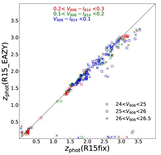
Through comparison with $z_{\mathrm{spec/grism}}$, S18 found that S14 photo-$z$s are reasonably well calibrated but suffer from a few systematic features. First, the comparison to the $z_{\mathrm{spec/grism}}$ revealed the presence of catastrophic redshift outliers, mostly in the form of galaxies at $2<z_{\mathrm{spec/grism}}<3$ that are assigned a redshift below $0.3$ (see also Figure 1 and also Section 5). This might be due to inaccurate template matching and degeneracies of the colour-redshift relation. Other issues that are not as prominent are noticeable redshift focusing (Wolf, 2009) at $1.4<$ photo-$z<1.6$ and the observation that the S14 photo-$z$s tend to generally be biased low compared to $z_{\mathrm{spec/grism}}$ at $z_{\mathrm{spec/grism}}>2.5$.

S18 found that the R15 photo-$z$s, calculated using bpz, performed better than the S14 photo-$z$s in terms of catastrophic outliers and the overall distribution, although R15 slightly overestimated photo-$z$s in the intervals of $1.0<$ photo-$z<1.7$ and $2.6<$ photo-$z<3.7$. Upon fixing the overestimated photo-$z$s by shifting the R15 photo-$z$s in these two intervals, S18 found that the fixed R15 photo-$z$s provide a sufficiently good approximation of the true redshifts. Hence, S18 utilised the fixed R15 photo-$z$s as a reference to obtain a statistical correction for the systematic features of the S14 photo-$z$s.

S18 had applied a statistical ad-hoc calibration method to correct for the systematic bias in the photo-$z$s distribution. The procedure is as follows; for each S14 galaxy with photo-$z<0.3$ and $V_{606}-I_{814}<0.2$ S18 add a randomly drawn offset from the comparison between S14 and the fixed R15 redshifts to its photo-$z$s. S18 also apply a statistical correction for the redshift focusing within the redshift range $1.4<$ photo-$z<1.6$ for galaxies with $V_{606}-I_{814}<0.1$, which are seen as most strongly affected, again randomly sampling from the corresponding $(z_{\mathrm{R15,fix}}-z_{\mathrm{S14}})_{i}$ offsets in the HUDF. For the latter correction S18 split the galaxies into two magnitude ranges ($24<V_{606}<25.5$ and $25.5<V_{606}<26.5$) given that the fainter galaxies appear to suffer from the redshift focusing effects more strongly. They have found that this statistical correction has resulted in a more unbiased distribution of photo-$z$s when compared against R15. The remaining systematic uncertainty of this correction estimated by S18 is $2.2\%$ (in terms of the average geometric lensing efficiency) for the photo-$z$s with an additional $1\%$ to account for variation between CANDELS fields.

In this paper, we investigate the origin of the outliers in the photo-$z$s calculated by S14 with an emphasis on the source population in weak lensing studies of high-redshift galaxy clusters. We also provide a more robust solution to correct for the systematic bias. We will mainly show results for the colour-magnitude-selected sample used in the analysis in S18. We will also show results for a purely magnitude-selected galaxy sample with $23<I_{\mathrm{814}}<27$ in Appendix A, which gives us an added insight to our analysis and might be of relevance for other weak lensing studies such as cosmic shear.

4 Methods

In this section, we explain the comparison metrics, as well as the error calculation that we use to evaluate the photo-$z$s quantitatively. Then, we elaborate on how we re-calculate the photo-$z$s using the algorithms bpz and eazy.

4.1 Comparison metrics

For our weak lensing analysis the most relevant metric of the redshift distribution is given by the mean geometric lensing efficiency, $\langle\beta\rangle$, which is defined as,

$$\langle\beta\rangle=\frac{\sum\beta(z_{i})w_{i}}{\sum w_{i}}\,,\,$$ (1)

where,

$$\beta=\mathrm{max}\left[0,\frac{D_{\mathrm{ls}}}{D_{\mathrm{s}}}\right].$$ (2)

Here, $w$ is the magnitude-dependent shape weight that is obtained through empirical fitting by S18 that down-weights contributions from faint galaxies, and $D_{\mathrm{s}}$ and $D_{\mathrm{ls}}$ indicate the angular diameter distances to the source and between the lens and the source, respectively. This is the most relevant metric of comparison for our studies because the cluster tangential shear scales with $\langle\beta\rangle$. Throughout this study, we assume the lens redshift to be at $z=0.9$ in accordance with the mean redshift of clusters in S18.

We then compare the $\langle\beta\rangle$ values computed from the investigated redshift distribution against a reference value, i.e. $\langle\beta_{\mathrm{ref}}\rangle$, computed from the reference distribution. We derive the relative bias of the mean geometric lensing efficiency by dividing the difference between the test $\langle\beta\rangle$ and $\langle\beta_{\mathrm{ref}}\rangle$ by $\langle\beta_{\mathrm{ref}}\rangle$. The errors on the relative bias are calculated by bootstrapping our galaxy sample. For each bootstrap sample realisation, we compute the $\langle\beta\rangle$ and $\langle\beta_{\mathrm{ref}}\rangle$ before taking the difference and normalising over $\langle\beta_{\mathrm{ref}}\rangle$.

The size of the error also depends on the whole distribution of redshifts. Considering the same sample size, a larger error means that there is a bigger dispersion in the bootstrapped calculation of the relative bias, which indicates that there is a bigger dispersion of $\langle\beta\rangle$$-\langle\beta_{\mathrm{ref}}\rangle$. This means that for a larger error, there is more overall scatter. For the cluster mass calibration, an error of $\lesssim 2\%$ is to be desired.

Another metric of comparison for the photo-$z$s is the catastrophic outlier fraction (COLF), where we defined a galaxy as outlier if it obeys $\left|\Delta z\right|/(1+z_{\mathrm{spec}})>0.6$. A high COLF is a sign that the photo-$z$s may be problematic, albeit being sometimes less biased than photo-$z$s with low COLF.

4.2 Photometric redshift algorithms

To investigate the cause of the difference of the S14 and R15 photo-$z$s, we re-calculate the photo-$z$s by employing the two template fitting algorithms, eazy (Brammer et al., 2008) which was applied by both S14 and R15, and bpz (Benítez, 2000), which was also used by R15. The photo-$z$s from both algorithms should match each other although some difference is possible. We summarise some of the most important differences between eazy and bpz below and refer to Hildebrandt et al. (2010) for further details.

The bpz and eazy codes both implement template-fitting algorithms to fit photometric data to a set of redshifted SEDs of galaxy templates. By integrating the likelihood employing a Bayesian prior they then determine the resulting photo-$z$s. For more details on template-fitting methods, see e.g. Bolzonella et al. (2000); Benítez (2000); Hildebrandt et al. (2010).

We employ the same eazy version that S14 utilised. This includes all the SED templates, priors and settings discussed in detail in Section 2.1.

We use the public bpz package, which employs an SED templates set that concentrates on the properties of high-redshift galaxies. It includes one elliptical, two spirals and an irregular type from Coleman et al. (1980), two starburst galaxies from Kinney et al. (1996), and two steep "blue" $25$Myr and $5$Myr simple stellar population model SEDs from Bruzual & Charlot (2003) that have been added to accommodate the large population of faint blue galaxies observed in the HUDF. An important feature in bpz is the interpolation between galaxy templates to mitigate the problem of incomplete template sets. The redshift prior that is employed in bpz is the default $I$-band based prior (see Section 2.2).

5 Results

Figure 1: Comparison of photo-$z$s in the HUDF including the peak photo-$z$s from eazy computed by the 3D-HST team in the GOODS-South field (left), the eazy photo-$z$s from the UVUDF project (middle), the bpz photo-$z$s from the UVUDF project (right, with small bias corrections applied, see text) to $z_{\mathrm{spec/grism}}$. Different colours and symbols correspond to different colour and magnitude ranges as indicated (based on the 3D-HST photometry).

5.1 S14 and R15 photo-$z$s comparison revisit

In this section we revisit the R15 and S14 photo-$z$s comparison, now including redshifts from MUSE.

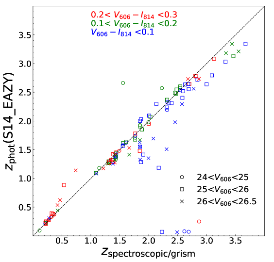
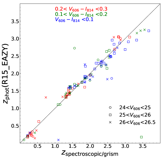
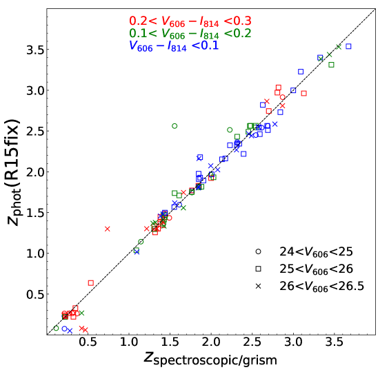
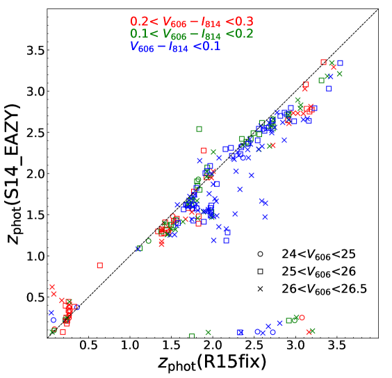
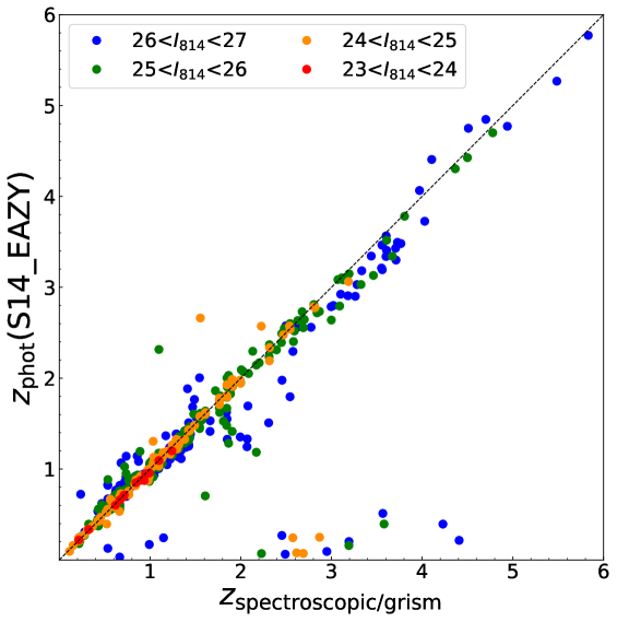
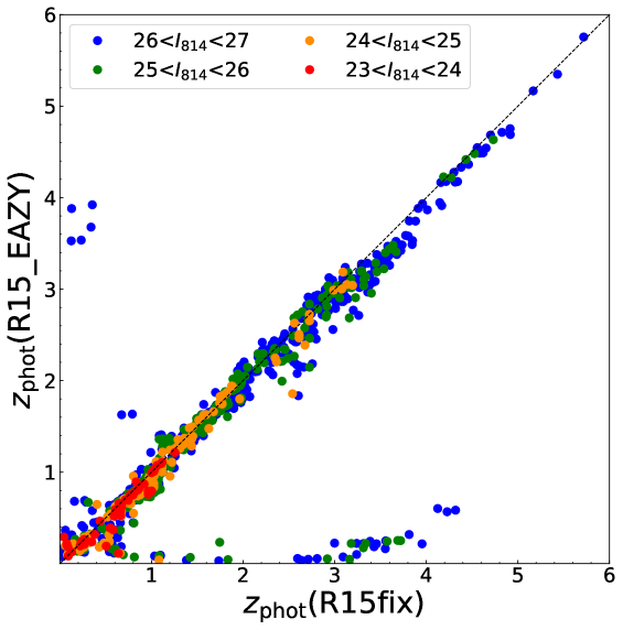
In the S18 comparison, S18 used the Momcheva et al. (2016) grism redshifts and S14 spec-$z$s compilation that includes 66 redshifts for the colour-and-magnitude-selected sample. Through the addition of the MUSE spec-$z$s (Inami et al., 2017) we have been able to include 128 galaxies in total. We perform the redshift comparison of the eazy photo-$z$s from S14 and R15, denoted as $z_{\mathrm{phot}}\texttt{(S14\_EAZY)}$ and $z_{\mathrm{phot}}\texttt{(R15\_EAZY)}$, to the $z_{\mathrm{spec/grism}}$ in Figure 1. Similarly to S18, we find that the $z_{\mathrm{phot}}\texttt{(S14\_EAZY)}$ are reasonably well calibrated but still show the same systematic features as stated in Section 3. We find that the $z_{\mathrm{phot}}\texttt{(R15\_BPZ)}$ still perform better, but are slightly biased high compared to $z_{\mathrm{spec/grism}}$. The bias in the photo-$z$s ranges $1.0<z<1.7$($2.6<z<3.2$) amounts to $0.081$($0.162$). We subtract the median offsets in these ranges ($0.081$ and $0.162$, respectively) from $z_{\mathrm{phot}}\texttt{(R15\_BPZ)}$, yielding $z_{\mathrm{phot}}\texttt{(R15fix)}$, which is shown in Figure 1. For comparison, $z_{\mathrm{phot}}\texttt{(R15\_EAZY)}$ also shows fewer catastrophic outliers than $z_{\mathrm{phot}}\texttt{(S14\_EAZY)}$ but suffers from a larger scatter around the one-to-one line compared to $z_{\mathrm{phot}}\texttt{(R15\_BPZ)}$.

Figure 2: The relative bias in the mean geometric lensing efficiency normalised to the $z_{\mathrm{spec/grism}}$ for the galaxies in our colour-and-magnitude-selected sample that have a match in the spec/grism-$z$s catalogue. The errors are determined via bootstrapping (see text). The right panel shows the corresponding COLF (see text).

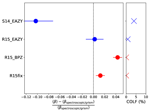
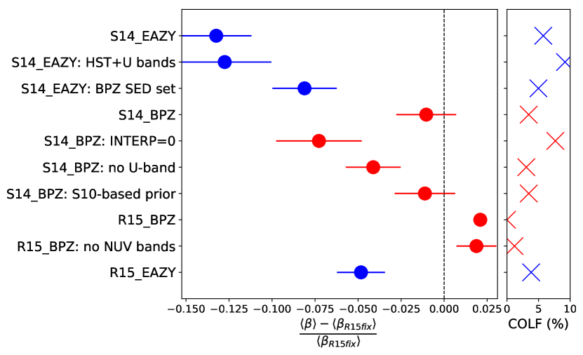
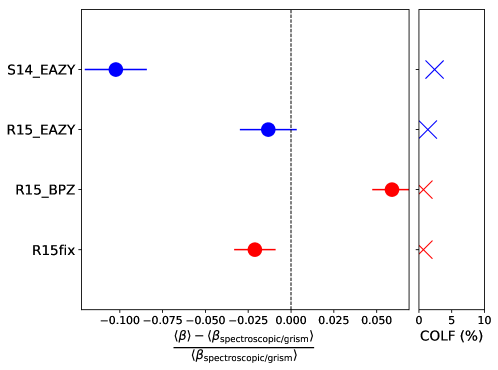
In Figure 2 we show the relative bias in $\langle\beta\rangle$ of $z_{\mathrm{phot}}\texttt{(S14\_EAZY)}$, $z_{\mathrm{phot}}\texttt{(R15\_EAZY)}$, $z_{\mathrm{phot}}\texttt{(R15\_BPZ)}$, and $z_{\mathrm{phot}}\texttt{(R15fix)}$ compared to $z_{\mathrm{spec/grism}}$ along with their corresponding COLF. We see that $z_{\mathrm{phot}}\texttt{(S14\_EAZY)}$ is indeed strongly biased low with a higher COLF compared to the rest. $z_{\mathrm{phot}}\texttt{(R15\_BPZ)}$ is biased high but with zero COLF. $z_{\mathrm{phot}}\texttt{(R15\_EAZY)}$ has a low COLF and $\langle\beta\rangle$ consistent with unbiased, however looking at the size of the error bar, it is much bigger than the error of $z_{\mathrm{phot}}\texttt{(R15\_BPZ)}$, which indicates that it has more scatter, as evident in Figure 1. To establish a new calibration sample, a tight correlation to $z_{\mathrm{spec/grism}}$ is desired. Therefore, we choose $z_{\mathrm{phot}}\texttt{(R15fix)}$, which is only slightly biased high with a smaller error bar. This corresponds to a $\sim+1\%$ overestimation of the $\langle\beta\rangle$, which we will discuss and take into account in Section 6.1. Importantly, $z_{\mathrm{phot}}\texttt{(R15fix)}$ does not suffer from the issue of catastrophic redshift outliers discussed in Section 3, which is essential for its use as a robust reference sample. In contrast, a significant, non-zero catastrophic redshift outlier fraction could depend on selection effects, which might differ between spectroscopic and photometric galaxy samples and lead to biased redshift calibrations when derived from incomplete reference samples.

However, we cannot exclude that spectroscopic selection effects might slightly affect our correction of the $z_{\mathrm{phot}}\texttt{(R15\_BPZ)}$ to $z_{\mathrm{phot}}\texttt{(R15fix)}$. For a conservative sensitivity analysis we assume a scenario in which the correction is preferentially required for galaxies with a spec/grism-$z$ estimate (on average these galaxies likely show stronger emission lines than random galaxies). If we conservatively assume that no correction would be required for half of the galaxies without spec/grism-$z$s, $\langle\beta\rangle$ would shift by $0.8\%$ only. We include this as a systematic uncertainty estimate in our final systematic error budget in Section 6.2.

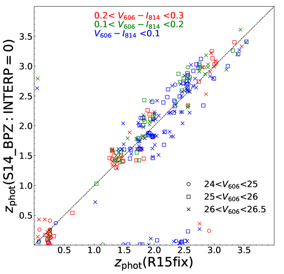
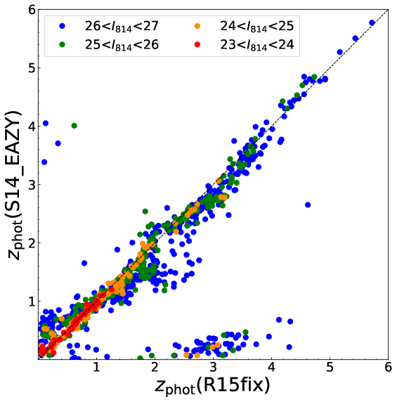
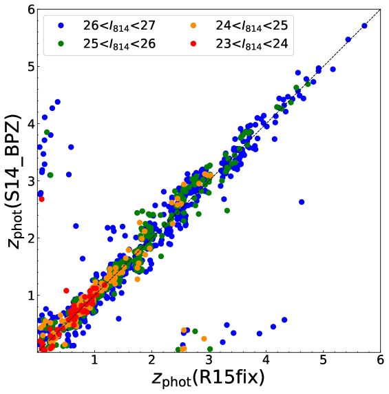
Comparing $z_{\mathrm{phot}}\texttt{(S14\_EAZY)}$ to $z_{\mathrm{phot}}\texttt{(R15fix)}$ in Figure 3 and assuming that $z_{\mathrm{phot}}\texttt{(R15fix)}$ represents the truth, shows that the $z_{\mathrm{phot}}\texttt{(S14\_EAZY)}$ catastrophic outliers are very asymmetric, where many galaxies with a high $z_{\mathrm{phot}}\texttt{(R15fix)}$ are assigned a low $z_{\mathrm{phot}}\texttt{(S14\_EAZY)}$, but not vice versa. At high redshift especially, it is obvious that the redshift distribution inferred from $z_{\mathrm{phot}}\texttt{(S14\_EAZY)}$ is strongly biased low.

Now that we have established $z_{\mathrm{phot}}\texttt{(R15fix)}$ as our new calibration sample, we will calculate the relative bias of various photo-$z$s calculations and normalise it to $\langle\beta_{\mathrm{R15fix}}\rangle$. In the following subsections, we will compare the relative bias/error of the tests we have done to investigate the source of the systematic features that are present in $z_{\mathrm{phot}}\texttt{(S14\_EAZY)}$.

Table 1: Explanation of the labels.

Label	Explanation
S14_eazy	The original photo-$z$s from S14. Bands used for the GOODS-South field are the ground-based $U$, $B$, $V$,
	$R$, $I$, $J$, $H$, $K_{s}$, 14 medium bands, $HST$ $F435W$, $F606W$, $F775W$, $F814W$, $F850LP$, $F125W$, $F140W$,
	$F160W$ bands, and $Spitzer$ $3.6,4.5,5.8,8\mu m$ bands
S14_eazy: $HST$ + $U$ bands	Calculated using only $HST$ bands and ground-based $U$-band
S14_eazy: bpz SED set	As S14_eazy: $HST$ + $U$ bands but changed the SED set from the ones employed by S14 to the ones
	from bpz
S14_bpz	Using bpz with all the changes as above, with "INTERP" set to 2 (see text)
S14_bpz: INTERP=0	As S14_bpz but "INTERP" is set to 0
S14_bpz: no $U$-band	Same as S14_bpz, but with $U$-band removed
S14_bpz: S10-based prior	Same as S14_bpz, but changed the prior from the default to an S10-based prior
R15_bpz	The original bpz photo-$z$s from R15
R15_bpz: no NUV bands	Calculated using bpz with the default settings (see text) using R15 data except for the $F225W$
	and $F275W$ bands removed
R15_eazy	The original eazy photo-$z$s from R15

Figure 3: Comparison of different sets of photo-$z$s to R15fix photo-$z$s for the colour-magnitude-selected sample, with symbols and colours similar to Figure 1.

Figure 4: Relative bias in the mean geometric lensing efficiency for the colour-magnitude-selected sample and different sets of $z_{\mathrm{phot}}$ compared to $z_{\mathrm{phot}}\texttt{(R15fix)}$. Description of the labels is given in Table 1. Errors are computed by bootstrapping the galaxy sample (see text), leading to hardly visible error-bars for (R15_BPZ), which differs from (R15fix) only because of the small redshift offsets described in Section 5.1. Blue(red) indicates that the photo-$z$s are calculated using eazy(bpz).

Figure 5: Same as in Figure 4 but divided into magnitude bins. The points in each magnitude bin are artificially spread out from the median value of each bin for clarity.

5.2 Tests using EAZY

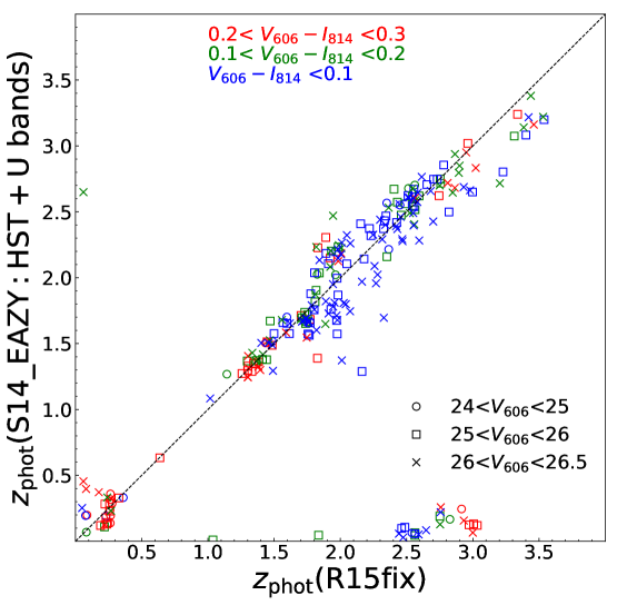
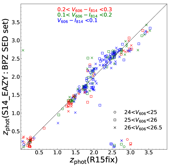
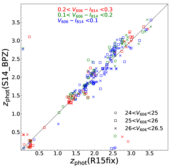
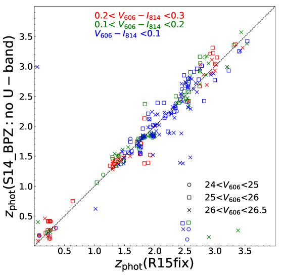
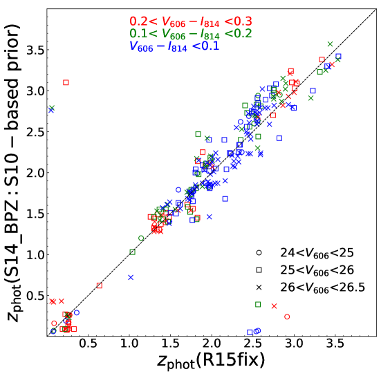
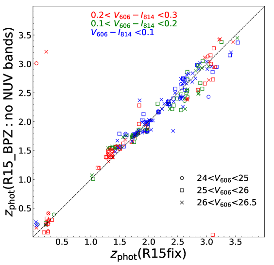
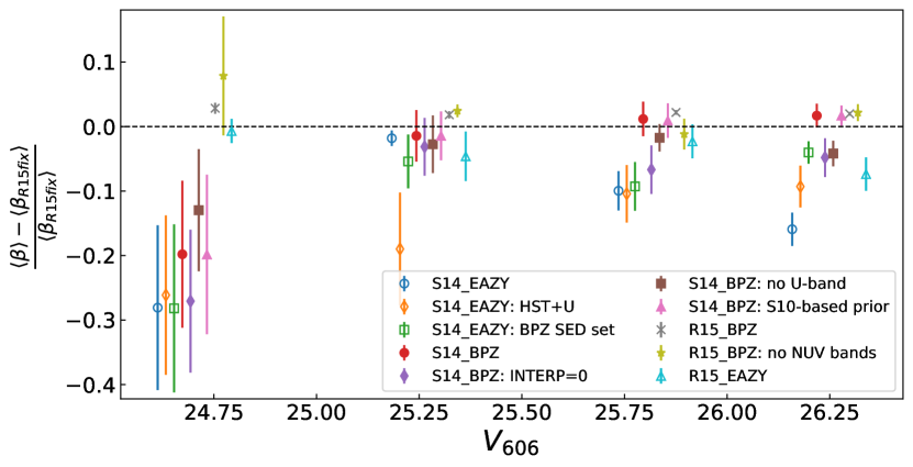
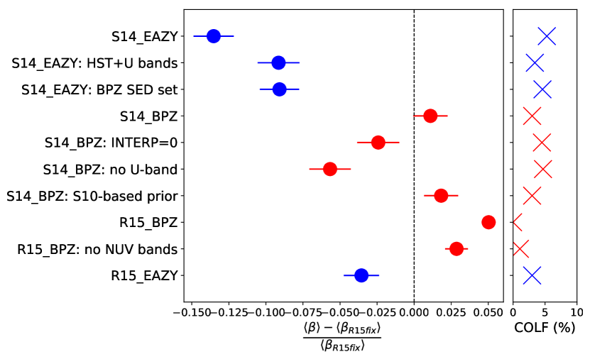
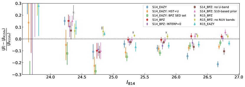
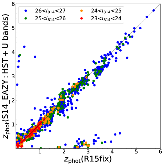
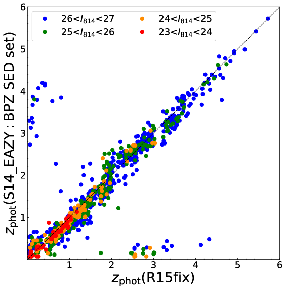
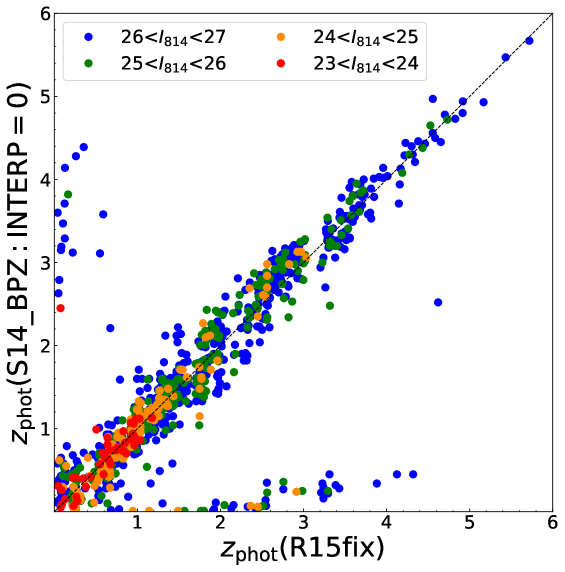
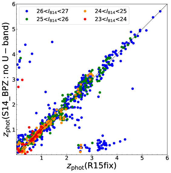
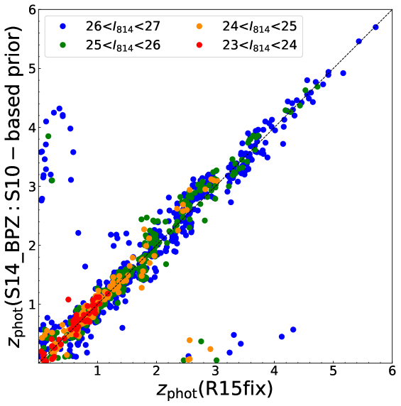
The first few tests involve photo-$z$ re-calculation using S14 photometric data while employing eazy. Figure 4 shows the relative bias/error to $\langle\beta_{\mathrm{R15fix}}\rangle$ and the corresponding COLF measured against R15fix for the colour-selected sample. We also divide our sample into $V_{\mathrm{606}}$ magnitude bins, shown in Figure 5, to identify if there is a trend with brightness. Lastly, we show the corresponding redshift comparison plots in Figure 3 to see if some features stand out as a function of redshift.

We find that by using only $HST$ bands and the ground-based $U$-band data from S14, we were able to reproduce the same relative bias as S14 within $0.5\%$. However, there is a higher COLF compared to S14. Referring to the top middle panel of Figure 3, we see that there is a slight up-scatter at $1.8<$ $z_{\mathrm{phot}}\texttt{(R15fix)}$$<2.8$ compared to the one-to-one line of mostly blue, $V_{606}-I_{814}<0.1$ galaxies, which partially compensates the low biasing due to the increase in asymmetric COLF. The findings of this test indicate that at the wavelength range and depth of the $HST$ weak lensing data, the auxiliary data from ground-based telescope surveys, that are not as as deep as the $HST$ data especially at the longer wavelength range, do not improve the photo-$z$ determination substantially. We did an intermediate test where we removed only the IRAC data but kept the remaining ground-based data, finding that this neither improves nor worsens the relative bias. This is supported by a few studies that have stated that adding mid-IR IRAC data makes the photo-$z$s worse or does not improve them significantly (Hildebrandt et al., 2010; Rafelski et al., 2015). Another intermediate test that we have done is changing the prior in eazy from the default $K_{\mathrm{s}}$-band to an $I$-band magnitude-based prior similar to the one employed in bpz, finding that this changes the bias by $0.5\%$ only. We keep the $I$-band prior used here for next tests. Similarly to removing the IRAC data, we find that including or removing the ground-based $H$-band and $K_{\mathrm{s}}$-band data does not change the results significantly, again suggesting that these data may be too shallow to improve the photo-$z$s at the depth of the weak lensing data.

We then change the SED templates set from the one employed by S14 to the one used in bpz. We found that this leads to a $5\%$ improvement of the relative bias compared to S14. This also leads to smaller error bars compared to (S14_EAZY:HST+U) and a slight decrease in COLF compared to S14. The redshift comparison plot (top right panel in Figure 3) shows that at $25<V_{606}<26$ galaxies seem to be focused at $z_{\mathrm{phot}}\texttt{(R15fix)}$ $\sim 1.9$. The relative bias decreases noticeably for the faintest magnitude bin when we change to this SED set. However, the overall relative bias of $-7.5\%$ is still not sufficient for our weak lensing analysis.

The geometric lensing efficiency is biased at a level of $-5\%$ for $z_{\mathrm{phot}}\texttt{(R15\_EAZY)}$, which is a weaker bias than obtained for any of the eazy analyses discussed above. This is also indicated by the tight correlation in the redshift comparison plot. There are fewer catastrophic outliers compared to all the tests discussed above. When investigated as function of magnitude (Figure 5), it is worth noting that the photo-$z$s are the least biased ones in the brightest bin.

5.3 Tests using BPZ

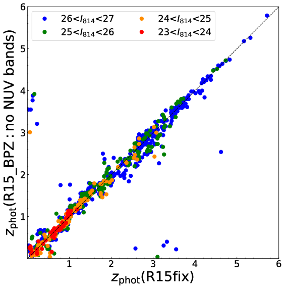
Up to this point, we have been unable to compute photo-$z$s that are consistent with being unbiased using eazy. We now employ bpz to re-calculate photo-$z$s. We first test our bpz implementation using R15 data. Since the SED templates that R15 used are private, the reliability of the photo-$z$s produced in this work relies heavily on how well we can reproduce the bpz photo-$z$s published by R15. Also, as we are using S14 data that do not include NUV bands, we need to see how significantly the NUV bands affect the resulting photo-$z$ distribution.

The relative bias of $z_{\mathrm{phot}}\texttt{(R15\_BPZ)}$ and the photo-$z$ set $z_{\mathrm{phot}}\texttt{(R15\_BPZ:no NUV bands)}$, which we calculate using our version of bpz and R15 data except the NUV bands, $F225W$ and $F275W$, seems to be at a similar level ($\sim+2\%$). There is some scatter around the one-to-one line although the overall correlation is very tight. There is increased scatter at higher redshifts than at lower redshifts in the redshift comparison plot. There are two catastrophic outliers at low $z_{\mathrm{phot}}\texttt{(R15fix)}$ and one at high $z_{\mathrm{phot}}\texttt{(R15fix)}$, which implies that our redshift estimates here do not produce a significant number of biased catastrophic outliers. The overall trend of (R15_BPZ:no NUV bands) is very similar to (R15_BPZ) in magnitude bins. We also run bpz using all data and found no significant difference for the photo-$z$s with or without NUV bands. This indicates that our bpz implementation is reliable and also that the NUV bands have no significant impact on the photo-$z$ determinations for our colour-magnitude-selected sample.

Next, we calculate photo-$z$s using only $HST$ bands and the ground-based $U$-band from S14, while employing the bpz SED set. The result is indicated as S14_BPZ in Figures 3, 4 and 5. The relative bias for this set compared to R15fix is found to be less than $2\%$. The COLF is low ($2\%$) and the outliers that are present are distributed more symmetrically with respect to the one-to-one line than for photo-$z$s calculated using eazy, leading to the low bias in $\langle\beta\rangle$.

The two algorithms used are very similar but they still differ in some effects, which then must be responsible for the differences. An important feature of bpz is the interpolation of templates. In the previous test, we set the INTERP function in bpz to the default value, INTERP=2. This means that for every adjacent SED, the code will produce two interpolated SEDs. This is likely important for fitting blue galaxies to the corresponding SEDs at high redshift, as the interpolated SEDs populate areas where there are significant gaps between the galaxy SED templates.

We find that the relative bias increases to $-7.5\%$ when we run bpz with INTERP=0. This is similar to what we got with $z_{\mathrm{phot}}\texttt{(S14\_EAZY: BPZ SED set)}$. The trend with magnitude is very similar to that set too (Figure 5). There is more scatter in the redshift comparison plot and a higher COLF than even compared to S14. This shows that this INTERP function significantly impacts the overall photo-$z$ performance. Our test for an even higher INTERP value reveals that there are no significant changes in the photo-$z$s.

We also run bpz on the S14 data with just $HST$ bands to study the impact of ground-based $U$-band data, with the result indicated by $z_{\mathrm{phot}}\texttt{(S14\_BPZ: no U-band)}$ in Figure 5. We find that it has a non-negligible impact on the relative bias. Removing the $U$-band tends to bias $\langle\beta\rangle$ low by $\sim-4\%$.

Lastly, we study the impact of modifying the redshift prior on the photo-$z$s distribution. We re-calibrated the redshift prior so that the redshift prior would be more accurate in describing our magnitude-selected sample. For this we employ the $I$-band magnitude-dependent fit to the redshift distribution of COSMOS30 galaxies (Ilbert et al., 2009) that was derived by Schrabback et al. (2010, S10 hereafter)

$$p(z|i)\propto\left(\frac{z}{z_{0}}\right)^{\alpha}\left(\exp{\left[-\left(\frac{z}{z_{0}}\right)^{\beta}\right]}+cu^{d}\exp{\left[-\left(\frac{z}{z_{0}}\right)^{\gamma}\right]}\right),\$$ (3)

where $z_{0}$ is computed from an assumed linear relation between the $I$-band magnitude and the median redshift, and $u=\mathrm{max}[0,(i-23)]$, with best-fitting parameters $(\alpha,\beta,c,d,\gamma)=(0.678,5.606,0.581,1.464)$. For the S10-based prior, we also choose to set the $f_{t}$ in Benítez (2000), which corresponds to the spectral fraction at reference magnitude $20$ for E/S0-type and Sbc/Scd-type templates to $0.05$ and $0.30$, respectively, instead of $0.35$ and $0.50$.

The S10-based redshift prior fits slightly better to the R15fix photo-$z$s distribution of our sample than the prior from bpz, both in terms of the median redshift difference of $0.13$ instead of $0.19$ (averaged over the magnitude bins) and the actual shape of the distribution. Figure 6 illustrates the shape of the S10-based prior and compares it to bpz default prior.

Figure 6: Redshift distribution of our magnitude-selected samples using the R15fix photo-$z$ histogram in green, fitted with the default prior from bpz (blue dashed line) and S10-based prior (orange solid line). For the default prior from bpz, we use the weighted average over the 3 types of galaxies.

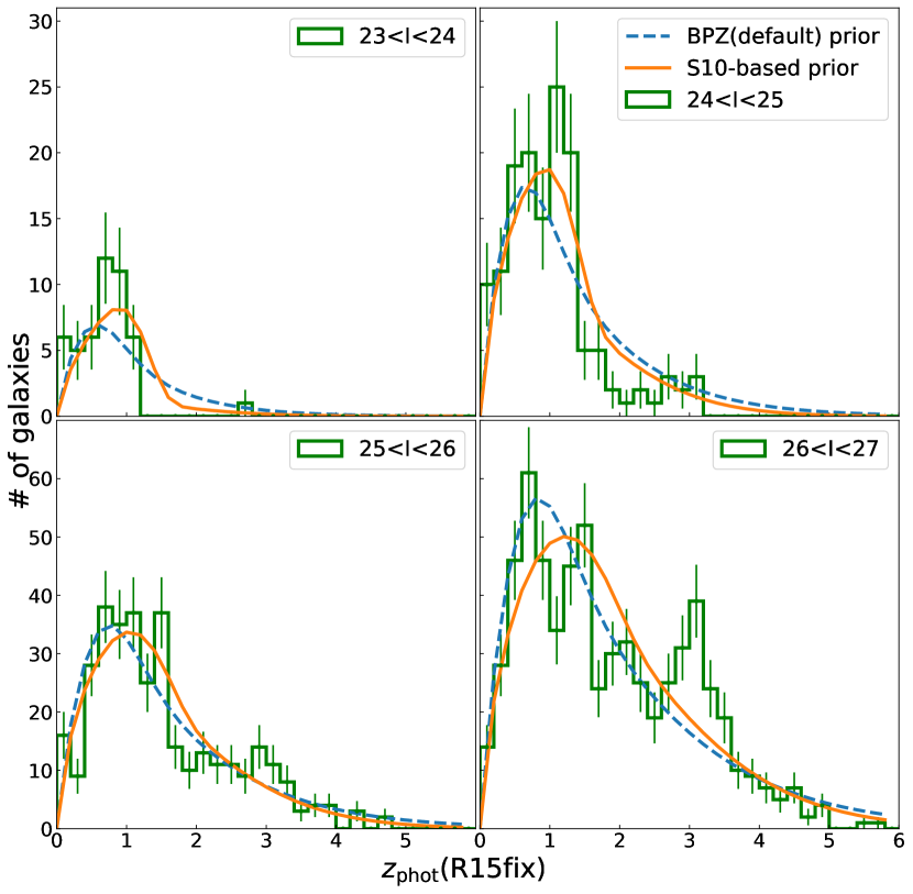
We find that there is not much change in the relative bias for the colour-magnitude-selected sample using the S10-based prior ($<0.5\%$) compared to $\langle\beta_{\mathrm{S14\_BPZ}}\rangle$. This indicates that the default prior in bpz, which was calibrated using HDFN CFRS spectroscopic data, is sufficient for our redshift analysis.

5.4 Using probability density distributions

Past studies have suggested that using the average photometric redshift posterior probability distribution $p(z)$ of all the galaxies gives a better approximation of the true redshift distribution than using the histogram of the single-peak point-estimated photometric redshifts (see e.g. Heymans et al., 2012; Benjamin et al., 2013; Bonnett, 2015). However, S18 found that the $p(z)$ of the S14 photo-$z$s cannot account for the systematic features that were identified in 5.1. Similarly, we recompute $\langle\beta\rangle$ using the $p(z)$, and compare the results to the $\langle\beta\rangle$ shown in Figure 4. We find that the bias computed using the $p(z)$ closely resembles the results from Figure 4. For example, (S14_BPZ: INTERP=0) and (S14_BPZ: no U-band) still yield a low $\langle\beta\rangle$ compared to S14_BPZ. Typically, $\langle\beta\rangle$ shift by $\lesssim 3\%$ only when switching from point estimates to averaged $p(z)$. Several reasons could be responsible for this behaviour, such as inaccuracies in the prior, systematic template or calibration issues, or violations of implicit Gaussian error assumptions.

6 Accuracy of the resulting redshift calibration

In this section, we discuss the accuracy of the resulting redshift calibration. For this, we also simulate shallower fields based of R15 photometry and estimate the resulting uncertainty from variations between CANDELS fields from the resulting $\langle\beta\rangle$ calculated using our updated photo-$z$s.

6.1 Simulating shallower fields

In this subsection, we investigate the impact of the varying noise levels in the photometric data of the different CANDELS fields on the photo-$z$ determination. One way to do this is to degrade the photometric data in deeper fields to match the noise level of the photometric data of shallower fields by adding noise. In particular, we added Gaussian noise to the R15 photometric data such that the noise level matches the depth of the five CANDELS fields in 3D-HST. For this, the total flux in the R15 catalogue is first converted to an aperture flux using the $F160W$ aperture-to-total ratio quoted in S14, then noise is added to the aperture flux. After that, these fluxes are converted back to total magnitudes using this ratio. We simulate a sufficient number of realisations of each noise level configuration. The result of the noise simulation is shown in Figure 7.

Figure 7: Relative bias of the mean geometric lensing efficiency of bpz photo-$z$s that we computed from R15 photometric data after adding noise to match the depth of the different CANDELS fields.

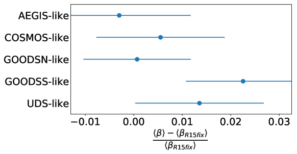
For the noise level of the GOODS-South field, we find a relative bias of $\langle\beta\rangle$ compared to R15fix of $+2.3\pm 1.3\%$, which is only marginally consistent with the bias we obtained using the actual S14 photometry in the overlapping HUDF area ($-1.0\pm 1.7\%$, S14_BPZ in Figure 4). However, it agrees well with the $+2.1\%$ bias obtained for R15_BPZ (see Figure 4). A cause for this might be the difference in photometric zero point offset calculation between S14 and R15. In the most extreme case, we found that in the $F435W$-band, the average magnitude offset is $-0.2$ mag in the S14 photometric catalogue compared to the R15 catalogue. The zero point offset is also inherited by the noise-added simulations, therefore systematically biasing the $\langle\beta\rangle$ the same way.

As visible in Figure 4, R15_BPZ leads to a bias of $+2.1\%$. As the average over all five noise configuration (see Figure 7) we find a small positive relative bias of $+0.8\pm 1.0\%$. This implies that the noise leads to a bias of $-1.3\pm 1.0\%$, which is consistent with S14_BPZ. This is compensated by the relative bias of $\langle\beta\rangle$ for R15fix compared to $z_{\mathrm{spec/grism}}$ (see Figure 2), which is $1.2\pm 0.7\%$. Combining these two together we expect a total relative bias of $0.1\pm 1.4\%$ for photo-$z$s computed with the S14_BPZ setup.

6.2 Accounting for variation between the CANDELS fields

We then re-calculate the photo-$z$s using S14 photometric data and our S14_BPZ setup for all five CANDELS fields. We use additional $G,B,I$, and $Z$-bands data from the ground for some of the CANDELS fields to supplement the absence of $F435W$, $F775W$, and $F850LP$ data. The summary of the bands used in the re-calculation of photo-$z$s is as follows, where we refer the reader to S14 regarding details on the individual bands:

• AEGIS: $U$, $G$, $I$, $Z$, $F606W$, $F814W$, $F125W$, $F140W$, $F160W$

• COSMOS: $U$, $B$, $I$, $Z$, $F606W$, $F814W$, $F125W$, $F140W$, $F160W$

• GOODSN: $U$, $F435W$, $F606W$, $F775W$, $F850LP$, $F125W$, $F140W$, $F160W$

• GOODSS: $U$, $F435W$, $F606W$, $F775W$, $F814W$, $F850LP$, $F125W$, $F140W$, $F160W$

• UDS: $U$, $B$, $I$, $Z$, $F606W$, $F814W$, $F125W$, $F140W$, $F160W$.

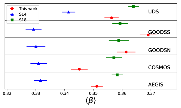
Here we also compare our $\langle\beta\rangle$ to the ones computed by S18 using their statistical correction to the photo-$z$s (see Figure 8). The mean $\langle\beta\rangle$ of the five CANDELS fields from our work is $0.3566\pm 0.0092$ which is consistent with the estimate $0.3595\pm 0.0026$ from the S18-corrected catalogues. Here the uncertainty on the mean is computed from the variation between the five fields, corresponding to a $2.6\%$ relative uncertainty for our results (the correction from S18). A part of the variation between the different fields comes from large-scale structure variations. This does, however, not explain the larger scatter for our results.

Naively we would expect the opposite behaviour, as S18 apply the same empirical redshift correction to all five CANDELS fields ignoring their variation in depth, which is in principle accounted for in our analysis. A possible explanation for the observed behaviour may be given by the fact that we include fewer bands in our analysis. This can lead to an increased scatter in the $\langle\beta\rangle$ between the five fields in two ways. First, fewer bands increase the impact of redshift focussing effects, which can differ between the different fields as they are not covered in exactly the same filters and with the same depth. Second, residual photometric calibration errors have a bigger impact on the photo-$z$s if fewer bands are used, whereas their impact averages out more if a larger number of filters is available.

Within our analysis framework we are not able to correct for these effects and therefore include the $2.6\%$ relative uncertainty in our systematic error budget. Added in quadrature to the uncertainty estimated in Sections 5.1 and 6.1 this yields a total relative systematic uncertainty of the $\langle\beta\rangle$ calibration of $3.0\%$.

Figure 8: Mean geometric lensing efficiency computed for the CANDELS fields using the original S14 catalogues, the empirically corrected catalogues from S18 and our new catalogues computed using the S14_BPZ setup.

6.3 Update to the S18 cluster masses

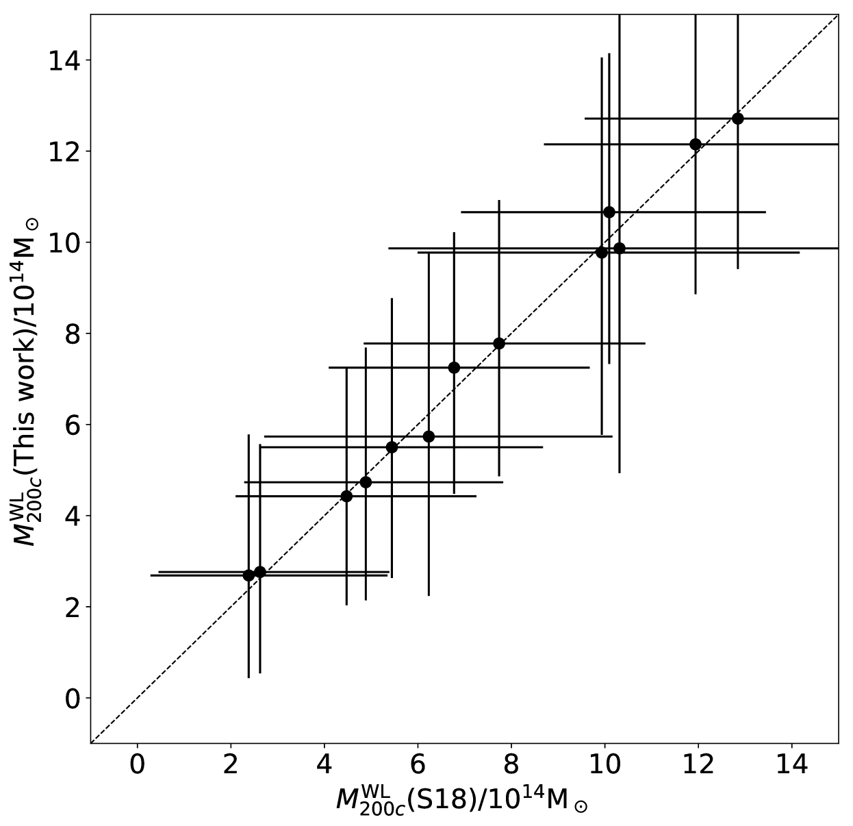
Using our new bpz CANDELS photo-$z$ catalogues for the redshift calibration we recompute the weak lensing masses of the high-redshift SPT-SZ clusters from S18 and compare them to the original estimates in Figure 9.

We find that the resulting mass estimates of the clusters in this work are very consistent with the mass estimates from S18: compared to S18 the masses shift by $+1\%$ on average.

Figure 9: Comparison of weak lensing mass estimates using the X-ray centres of this work versus S18. The mass constraints are based on NFW fits to the reduced shear profiles using scales $500\mathrm{\,kpc}<r<1.5$ Mpc employing the Diemer & Kravtsov (2015) $c(\mathrm{M})$ relation for over-densities in $200\mathrm{c}$, and correcting for mass modelling bias as done by S18. All errors are statistical $68\%$ uncertainties, including the contributions from shape noise, uncorrelated large-scale, and line-of-sight variations in the redshift distribution. See S18 for further details on the weak lensing mass measurements.

7 Conclusions

Firstly, through comparison with $z_{\mathrm{spec/grism}}$, we have established that very deep photo-$z$s from R15 constitute a good calibration sample that solves the problem of incomplete spec-$z$s for faint, high-redshift galaxies. Here we applied a small bias correction to the R15 photo-$z$s, and denoted these corrected photo-$z$s as R15fix.

When comparing the R15 and S14 photo-$z$s, we found that S14 suffers from systematic features, most importantly catastrophic outliers, which systematically bias the distribution of the photo-$z$s low. This bias of the photo-$z$s is problematic for weak lensing studies as biased photo-$z$s will lead to a biased interpretation of the weak lensing signal. For our colour-magnitude-selected sample, the relative bias in $\langle\beta\rangle$ of the S14 photo-$z$s compared to $z_{\mathrm{phot}}\texttt{(R15fix)}$ is $-13.2\%$.

In general, the absolute value of a bias is less of concern since it can be compensated in a cosmological analysis. Instead, it is the accuracy with which the bias can be determined that propagates into the systematic error budget of the cosmological constraints. In order to better constrain this accuracy, we have studied the cause of the systematic features by re-calculating photo-$z$s to test the impact of differences in the analysis and the data between the S14 and R15 photo-$z$s. We have found that, although the S14 data have lower S/N compared to R15, we are able to achieve a low relative bias of less than $2\%$ by using bpz instead of eazy. Apart from changing the SED set, we found that the interpolation of the SED set as implemented in bpz has the biggest impact on the relative bias for the colour-magnitude-selected sample. We also found that the inclusion of $U$-band data from ground-based telescopes is crucial to obtain accurate photo-$z$ distributions. FIR IRAC data and the other ground-based data only have a small impact on the relative bias.

For bpz we also tested the use of an alternative prior based on COSMOS-30 photo-$z$s, finding that it has only a minor impact. Using eazy we tried to match the bpz properties, employing the same templates and priors. Nevertheless, we have been unable to obtain unbiased results with eazy. Using the averaged probability density distribution of the photo-$z$s instead of using single-peak point-estimated photo-$z$s did not change the bias results.

We investigated the impact of noise by degrading the R15 HUDF photometry to the depth of the different CANDELS fields. Combining these results with the estimates from the initial spectroscopic comparison we expect that our setup running bpz on S14 data should yield unbiased estimates of $\langle\beta\rangle$ with a systematic uncertainty of $1.4\%$. Using this setup we then recomputed the photo-$z$s for all five CANDELS fields. Here we detected a larger field-to-field variation in the $\langle\beta\rangle$ compared to S18, which may be caused by the inclusion of fewer bands in our analysis, leading to a total systematic uncertainty of the $\langle\beta\rangle$ calibration of $2.9\%$. Using our updated CANDELS catalogues as reference sample we recomputed the cluster mass estimates from S18, finding an average increase of the masses by $+1\%$.

In the future, we will apply these updated photo-$z$s in combination with an updated shear calibration (Hernández-Martín et al. (submitted)) and extended $HST$ data sets, e.g. from the SPT ACS snapshot survey (Schrabback et al. in prep) to further improve the mass calibration of high-redshift galaxy clusters.

Data availability

The data underlying this study are available in the links within the article. The photo-$z$ catalogues generated are available on request to the corresponding author, SFR.

Appendix A Result for a purely magnitude-selected sample

Although the redshift offset in $z_{\mathrm{phot}}\texttt{(R15fix)}$ is formulated using the colour-magnitude-selected sample, we find that it is still appropriate for the purely magnitude-selected sample. The corresponding plots for the purely magnitude-selected sample are shown in Figures 10 and 11.

Figure 10: Similar to Figure 1 but with purely magnitude selection applied. Different colours correspond to magnitude ranges as indicated.

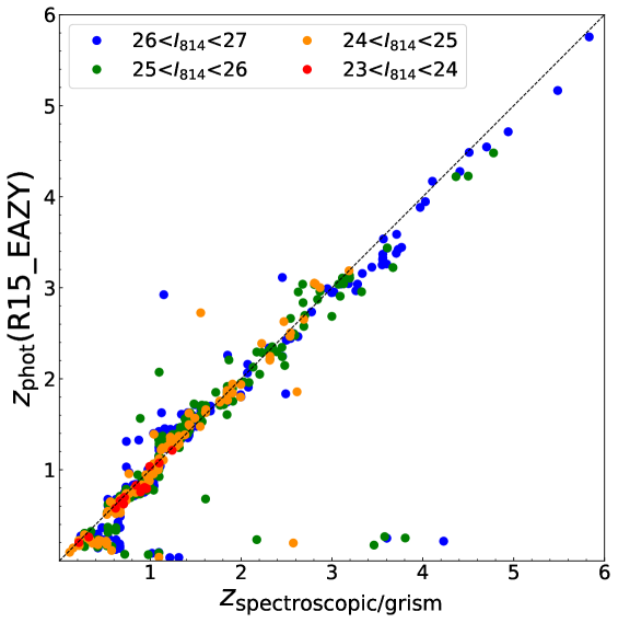
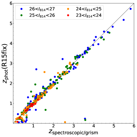
The overall trend is quiet similar to what is seen in the colour-magnitude-selected sample. Applying the shifts is seen to slightly overcompensate the biased $\langle\beta\rangle$(refer to label R15fix in Figure 11). In Figure 10 we see that $z_{\mathrm{phot}}\texttt{(S14\_EAZY)}$ indeed suffers from outliers that are catastrophically biased low including fairly bright galaxies with $24<I_{\mathrm{814}}<25$. Using deeper data with eazy reduces the catastrophic outliers but also does not completely remove them (refer to label $z_{\mathrm{phot}}\texttt{(R15\_EAZY)}$ in Figure 10). $z_{\mathrm{phot}}\texttt{(R15fix)}$ have the least remaining catastrophic outliers, which confirms our choice of using these photo-$z$s as our new calibration sample. Different to the spec/grism-$z$s sample it does not suffer from incompleteness at relevant depths needed for weak lensing studies.

Figure 11: The relative bias in the mean geometric lensing efficiency normalised to the $z_{\mathrm{spec/grism}}$ of our purely magnitude-selected sample. The errors are from bootstrapping (see text). The right panel shows the corresponding COLF (see text).

Figure 12: Similar to Figure 4 but for a purely magnitude-selected sample.

Figure 13: Similar to Figure 5 but for a purely magnitude-selected sample.

Figure 14: Comparison of the purely magnitude-selected sample photo-$z$s to R15fix photo-$z$s with symbols and colours similar to Figure 1.

The total relative bias and error, COLF, relative bias in magnitude bins, and redshift comparison plots for the purely magnitude-selected sample are shown in Figure 12, 13 and 14. Overall, the trend that eazy underestimates and bpz tend to slightly overestimate the mean $\langle\beta\rangle$ is also shown here with biases of $\sim-15\%$ for $z_{\mathrm{phot}}\texttt{(S14\_EAZY)}$ and $\sim+5\%$ for $z_{\mathrm{phot}}\texttt{(R15\_BPZ)}$. Note that the purely magnitude-selected sample includes significantly fainter galaxies, so we can see here the result of our test on much noisier data. We find that removing ground bands and FIR-bands leads to a bigger improvement for the relative bias compared to the analysis for the colour-magnitude-selected sample. Changing the SEDs set after that did not have any significant impact on the overall bias. However, it turns out that the SEDs used by eazy seem to work better than bpz’s SEDs set for high S/N data, while the opposite is the case for low S/N data (see Figure 13). This confirms the fact that bpz’s SED are more focused on the high-redshift blue, star-bursting galaxies. We manage to get a relatively unbiased mean $\langle\beta\rangle$ after switching to bpz. However, unlike for the colour-magnitude-selected sample this cannot be fully explained by the template interpolation. A possible additional cause could be that the template error function in eazy, which is an exclusive function in the algorithm, is not suited for the SED templates used by bpz. Therefore, it cannot function optimally with very low S/N data.

The impact of $U$-band is more significant in this sample. The difference in the relative bias of the test with $U$-band compared to no $U$-band increases as the $I$-band magnitude increases, especially at the faintest bin where we have the largest number of galaxies. This shows that extending the wavelength range to $U$-band is crucial when studying galaxies that are fainter and more distant in future studies. We see also a small difference in our no NUV bands bpz photo-$z$s and $z_{\mathrm{phot}}\texttt{(R15\_BPZ)}$. They mainly differ in the brighter magnitude bins and not in the faint bins. This might be due to the fact that the NUV bands are not as deep as the rest of the R15 data.

Modifying the redshift prior shows to have a very small impact on the photo-$z$ determination for the magnitude-selected sample.

References

- Allen et al. (2011) Allen S. W., Evrard A. E., Mantz A. B., 2011, ARA&A, 49, 409
- Applegate et al. (2016) Applegate D. E., et al., 2016, MNRAS, 457, 1522
- Bacon et al. (2010) Bacon R., et al., 2010, in Proc. SPIE. p. 773508, doi:10.1117/12.856027
- Bacon et al. (2015) Bacon R., et al., 2015, A&A, 575
- Beckwith et al. (2006) Beckwith S. V. W., et al., 2006, AJ, 132, 1729
- Benítez (2000) Benítez N., 2000, ApJ, 536, 571
- Benítez et al. (2009) Benítez N., et al., 2009, ApJ, 692, L5
- Benjamin et al. (2013) Benjamin J., et al., 2013, MNRAS, 431, 1547
- Blaizot et al. (2005) Blaizot J., Wadadekar Y., Guiderdoni B., Colombi S. T., Bertin E., Bouchet F. R., Devriendt J. E. G., Hatton S., 2005, MNRAS, 360, 159
- Bleem et al. (2015) Bleem L. E., et al., 2015, ApJS, 216, 27
- Bocquet et al. (2019) Bocquet S., et al., 2019, ApJ, 878, 55
- Bolzonella et al. (2000) Bolzonella M., Miralles J. M., Pelló R., 2000, A&A, 363, 476
- Bonnett (2015) Bonnett C., 2015, MNRAS, 449, 1043
- Bouwens et al. (2011) Bouwens R. J., et al., 2011, ApJ, 737, 90
- Brammer et al. (2008) Brammer G. B., van Dokkum P. G., Coppi P., 2008, ApJ, 686, 1503
- Brammer et al. (2012) Brammer G. B., et al., 2012, ApJS, 200, 13
- Brinchmann et al. (2017) Brinchmann J., et al., 2017, A&A, 608, A3
- Bruzual & Charlot (2003) Bruzual G., Charlot S., 2003, MNRAS, 344, 1000
- Chang et al. (2019) Chang C., et al., 2019, MNRAS, 482, 3696
- Coe et al. (2006) Coe D., Benítez N., Sánchez S. F., Jee M., Bouwens R., Ford H., 2006, AJ, 132, 926
- Coleman et al. (1980) Coleman G. D., Wu C.-C., Weedman D. W., 1980, ApJS, 43, 393
- Crampton et al. (1995) Crampton D., Fevre O. L., Lilly S. J., Hammer F., 1995, ApJ, 455, 96
- Diemer & Kravtsov (2015) Diemer B., Kravtsov A. V., 2015, ApJ, 799, 108
- Dietrich et al. (2019) Dietrich J. P., et al., 2019, MNRAS, 483, 2871
- Ellis et al. (2013) Ellis R. S., et al., 2013, ApJ, 763, L7
- Fioc & Rocca-Volmerange (1997) Fioc M., Rocca-Volmerange B., 1997, A&A, 500, 507
- Galametz et al. (2013) Galametz A., et al., 2013, ApJS, 206, 10
- Grogin et al. (2011) Grogin N. A., et al., 2011, ApJS, 197, 35
- Heymans et al. (2012) Heymans C., et al., 2012, MNRAS, 427, 146
- Hikage et al. (2019) Hikage C., et al., 2019, PASJ, 71, 43
- Hildebrandt et al. (2010) Hildebrandt H., et al., 2010, A&A, 523, A31
- Hildebrandt et al. (2017) Hildebrandt H., et al., 2017, MNRAS, 465, 1454
- Hildebrandt et al. (2018) Hildebrandt H., et al., 2018, A&A submitted (also in arXiv e-prints), p. arXiv:1812.06076
- Hinshaw et al. (2013) Hinshaw G., et al., 2013, ApJS, 208, 19
- Hoekstra et al. (2011) Hoekstra H., Donahue M., Conselice C. J., McNamara B. R., Voit G. M., 2011, ApJ, 726, 48
- Hoekstra et al. (2015) Hoekstra H., Herbonnet R., Muzzin A., Babul A., Mahdavi A., Viola M., Cacciato M., 2015, MNRAS, 449, 685
- Ilbert et al. (2009) Ilbert O., et al., 2009, ApJ, 690, 1236
- Inami et al. (2017) Inami H., et al., 2017, A&A, 608, A2
- Jee et al. (2011) Jee M. J., et al., 2011, ApJ, 737, 59
- Jee et al. (2016) Jee M. J., Tyson J. A., Hilbert S., Schneider M. D., Schmidt S., Wittman D., 2016, ApJ, 824, 77
- Kinney et al. (1996) Kinney A. L., Calzetti D., Bohlin R. C., McQuade K., Storchi-Bergmann T., Schmitt H. R., 1996, ApJ, 467, 38
- Koekemoer et al. (2011) Koekemoer A. M., et al., 2011, ApJS, 197, 36
- Koekemoer et al. (2013) Koekemoer A. M., et al., 2013, ApJS, 209, 3
- Leauthaud et al. (2010) Leauthaud A., et al., 2010, ApJ, 709, 97
- Lilly et al. (1995) Lilly S. J., Fevre O. L., Crampton D., Hammer F., Tresse L., 1995, ApJ, 455, 50
- Mantz et al. (2014) Mantz A. B., Allen S. W., Morris R. G., Rapetti D. A., Applegate D. E., Kelly P. L., von der Linden A., Schmidt R. W., 2014, MNRAS, 440, 2077
- Maraston (2005) Maraston C., 2005, MNRAS, 362, 799
- Marrone et al. (2012) Marrone D. P., et al., 2012, ApJ, 754, 119
- McClintock et al. (2019) McClintock T., et al., 2019, MNRAS, 482, 1352
- Momcheva et al. (2016) Momcheva I. G., et al., 2016, ApJS, 225, 27
- Oesch et al. (2010a) Oesch P. A., et al., 2010a, ApJ, 709, L16
- Oesch et al. (2010b) Oesch P. A., et al., 2010b, ApJ, 709, L21
- Okabe & Smith (2016) Okabe N., Smith G. P., 2016, MNRAS, 461, 3794
- Rafelski et al. (2015) Rafelski M., et al., 2015, AJ, 150, 31
- Reiprich & Böhringer (2002) Reiprich T. H., Böhringer H., 2002, ApJ, 567, 716
- Rozo et al. (2010) Rozo E., et al., 2010, ApJ, 708, 645
- Schellenberger & Reiprich (2017) Schellenberger G., Reiprich T. H., 2017, MNRAS, 471, 1370
- Schlegel et al. (1998) Schlegel D. J., Finkbeiner D. P., Davis M., 1998, ApJ, 500, 525
- Schrabback et al. (2010) Schrabback T., et al., 2010, A&A, 516, A63
- Schrabback et al. (2018) Schrabback T., et al., 2018, MNRAS, 474, 2635
- Skelton et al. (2014) Skelton R. E., et al., 2014, ApJS, 214, 24
- Speagle & Eisenstein (2017) Speagle J. S., Eisenstein D. J., 2017, MNRAS, 469, 1205
- Stern et al. (2019) Stern C., et al., 2019, MNRAS, 485, 69
- Sunyaev & Zeldovich (1970) Sunyaev R. A., Zeldovich Y. B., 1970, Comments on Astrophysics and Space Physics, Vol. 2, p.66, 2, 66
- Sunyaev & Zeldovich (1972) Sunyaev R. A., Zeldovich Y. B., 1972, Comments on Astrophysics and Space Physics, Vol. 4, p.173, 4, 173
- Tanaka et al. (2018) Tanaka M., et al., 2018, PASJ, 70, S9
- Teplitz et al. (2013) Teplitz H. I., et al., 2013, AJ, 146, 159
- Thölken et al. (2018) Thölken S., et al., 2018, A&A, 610, A71
- Troxel et al. (2018) Troxel M. A., et al., 2018, MNRAS, 479, 4998
- Whitaker et al. (2011) Whitaker K. E., et al., 2011, ApJ, 735, 86
- Williams et al. (1996) Williams R. E., et al., 1996, AJ, 112, 1335
- Wolf (2009) Wolf C., 2009, MNRAS, 397, 520
- Wuyts et al. (2008) Wuyts S., Labbé I., Förster Schreiber N. M., Franx M., Rudnick G., Brammer G. B., van Dokkum P. G., 2008, ApJ, 682, 985
- de Jong et al. (2013) de Jong J. T. A., Verdoes Kleijn G. A., Kuijken K. H., Valentijn E. A., Consortiums K., Astro-WISE 2013, Experimental Astronomy, 35, 25
- van Uitert et al. (2018) van Uitert E., et al., 2018, MNRAS, 476, 4662
- von der Linden et al. (2014) von der Linden A., et al., 2014, MNRAS, 443, 1973