1 Introduction

The primary obstacle towards scaling distributed optimization algorithms is the significant communication cost both in terms of the number of communication rounds and the amount of exchanged data per round. To significantly reduce the number of communication rounds, a practical solution is to trade-off local computation for less communication via periodic averaging [62, 48]. In particular, the local SGD algorithm [48, 53, 60] alternates between a fixed number of local updates and one step of synchronization which is shown to enjoy the same convergence rate as its fully synchronous counterpart, while significantly reducing the number of communication rounds.

A fundamentally different solution to scale up distributed optimization algorithms is to reduce the size of the communicated message per communication round. This problem is especially exacerbated in edge computing where the worker devices (e.g., smartphones or IoT devices) are remotely connected, and communication bandwidth and power resources are limited. For instance, ResNet [16] has more than 25 million parameters, so the communication cost of sending local models through a computer network could be prohibitive. The current methodology towards reducing the size of messages is to communicate compressed local gradients or models to the central server by utilizing a quantization operator [3, 6, 52, 58, 56, 51, 41], sparsification schema [49, 33, 58, 4], or composition of both [5].

	Objective function
Reference	Nonconvex	PL/Strongly Convex	General Convex
QSPARSE[5]	$R\!=\!O\left(\frac{q+1}{\epsilon^{{3}/{2}}}\right)$ $\tau\!=\!O\left(\frac{1}{m(q+1)\sqrt{\epsilon}}\right)$	$R=O\left({\color[rgb]{0,0,0}\definecolor[named]{pgfstrokecolor}{rgb}{0,0,0}\pgfsys@color@gray@stroke{0}\pgfsys@color@gray@fill{0}\kappa}\frac{q+1}{\sqrt{\epsilon}}\right)$ $\tau=O\left(\frac{1}{m\left(q+1\right)\sqrt{\epsilon}}\right)$	$-$
FedPAQ[41]	$R=O\left(\frac{1}{\epsilon}\right)$ $\tau=O\left(\frac{(\frac{q}{m})^{2}+1}{\epsilon}\right)$	$R=O\left(m+\frac{q+1}{m\epsilon}\right)$ $\tau=O\left(1\right)$	$-$
Theorem 5.1	$\boldsymbol{R=O\left(\frac{1}{\epsilon}\right)}$ $\boldsymbol{\tau=O\left(\frac{q+1}{m\epsilon}\right)}$	$\boldsymbol{R=O\left(\kappa\left(\frac{q}{m}+1\right)\log\left(\frac{1}{\epsilon}\right)\right)}$ $\boldsymbol{\tau=O\left(\frac{\left(q+1\right)}{m\left(\frac{q}{m}+1\right)\epsilon}\right)}$	$\boldsymbol{R\!=\!O\left(\frac{1+\frac{q}{m}}{\epsilon}{\color[rgb]{0,0,0}\definecolor[named]{pgfstrokecolor}{rgb}{0,0,0}\pgfsys@color@gray@stroke{0}\pgfsys@color@gray@fill{0}\log\left(\frac{1}{\epsilon}\right)}\right)}$ $\boldsymbol{\tau\!=\!O\left(\frac{\left(q+1\right)^{2}}{m\left(\frac{q}{m}+1\right)^{2}\epsilon^{2}}\right)}$

Table 1: Comparison of results with compression and periodic averaging in the homogeneous setting. Here, $m$ is the number of devices, $q$ is compression distortion constant, $\kappa$ is condition number, $\epsilon$ is target accuracy, $R$ is the number of communication rounds, and $\tau$ is the number of local updates. QSPARSE [5] has the assumption of bounded gradient, while FedPAQ [41] and our proposed algorithm do not have such assumption.

Despite significant progress in improving both aspects of communication efficiency [22, 49, 6, 50], there still exists a huge gap in our understanding of these approaches in federated learning, in particular for the cases that both compression and periodic averaging techniques are applied simultaneously. In terms of reducing communication rounds, a few recent attempts were able to reduce the frequency of synchronizing locally evolving models [13, 23], which are not improvable in general [63]. This necessitates that further improvement in communication efficiency needs to be explored by reducing the size of communicated messages. We highlight that compressed communication is of further importance to accelerate training non-convex objectives as it requires significantly more communication rounds to converge compared to distributed convex optimization. Furthermore, most existing methods are analyzed for homogeneous data and our understanding of the efficiency of these methods in the heterogeneous case is lacking.

In light of the above issues, the key contribution of this paper is the introduction and analysis of simple variants of local SGD with compressed communicationP  without compromising the attainable guarantees. The proposed algorithmic ideas accommodate both homogeneous and heterogeneous data distribution settings with the obtained rates summarized in Table 1 and Table 2, respectively. In the homogeneous case, with a tight analysis of a simple quantized variant of local SGD, we show that not only our proposed method improves the complexity bounds for algorithms with compression (Table 1), but also outperforms the complexity bounds for non-compressed counterparts in terms of the number of communication rounds (Table 5). In the heterogeneous case, we argue that in the presence of compression (quantization or sparsification), locally updating models via local gradient information could lead to a significant drift among local models, which shed light on designing a quantized variant of local SGD that tracks local gradient information at local devices. We show that this simple gradient tracking idea leads to a method that outperforms state-of-the-art methods with compression for the heterogeneous setting (Table 2) and it can even compensate for the noise introduced by compression and lead to the best-known convergence rates for convex and non-convex settings under perfect communication, i.e., no compression (Table 6).

	Objective function
Reference	Nonconvex	PL/Strongly Convex	General Convex
QSPARSE[5]	$R=O\left(\frac{q+1}{\epsilon^{{3}/{2}}}\right)$ $\tau=O\left(\frac{1}{m(q+1)\sqrt{\epsilon}}\right)$	$R=O\left({\color[rgb]{0,0,0}\definecolor[named]{pgfstrokecolor}{rgb}{0,0,0}\pgfsys@color@gray@stroke{0}\pgfsys@color@gray@fill{0}\kappa}\frac{q+1}{\sqrt{\epsilon}}\right)$ $\tau=O\left(\frac{1}{m\left(q+1\right)\sqrt{\epsilon}}\right)$	$-$
Theorem 5.2	$\boldsymbol{R=O\left(\frac{q+1}{\epsilon}\right)}$ $\boldsymbol{\tau=O\left(\frac{1}{m\epsilon}\right)}$	$\boldsymbol{R=O\left(\kappa\left({q}+1\right)\log\left(\frac{1}{\epsilon}\right)\right)}$ $\boldsymbol{\tau=O\left(\frac{1}{m\epsilon}\right)}$	$\boldsymbol{R=O\left(\frac{1+{q}}{\epsilon}{\color[rgb]{0,0,0}\definecolor[named]{pgfstrokecolor}{rgb}{0,0,0}\pgfsys@color@gray@stroke{0}\pgfsys@color@gray@fill{0}\log\left(\frac{1}{\epsilon}\right)}\right)}$ $\boldsymbol{\tau=O\left(\frac{1}{m\epsilon^{2}}\right)}$

Table 2: Comparison of results with compression and periodic averaging in the heterogeneous setting. QSPARSE [5] has the assumption of bounded gradient, while our proposed algorithm does not.

Contributions. We summarize the main contributions of this paper below:

• Homogeneous local distributions: To keep the analysis simple yet insightful, we start with a quantized variant of federated averaging algorithm and analyze its convergence for non-convex, strongly convex and general convex objectives. As demonstrated in Table 1, the obtained rates is novel for convex objectives to the best of our knowledge, and improves the best known bounds in [41] and  [5] for general non-convex and strongly convex objectives, respectively.

• Heterogeneous local distributions: For the heterogeneous setting, we propose federated averaging with compression and local gradient tracking, dubbed as FedCOMGATE algorithm, and establish its convergence rates for general non-convex, strongly convex or PL, and convex objectives. The obtained rates improve upon the results reported in [5] for general non-convex and strongly-convex objectives. The obtained rates for general convex functions are novel to the best of our knowledge.

• We verify our theoretical results through various extensive experiments on different real federated datasets that demonstrate the practical efficacy of our methods.

2 Problem Setup

In this paper we focus on a federated architecture, where $m$ users aim to learn a global model in a collaborative manner without exchanging their data points with each other. Moreover, we assume that users (computing units) can only exchange information via a central unit (server) which is connected to all users. The optimization problem that the users try to solve can be written as

$$\min_{\boldsymbol{w}\in\mathbb{R}^{d}}f(\boldsymbol{w})\triangleq\frac{1}{m}\sum_{j=1}^{m}f_{j}(\boldsymbol{w})$$ (1)

where $f_{j}:\mathbb{R}^{d}\to\mathbb{R}$ is the loss function corresponding to user $j$. We further assume that the local objective function of each user $j$ is the expected loss over the set of data points of node $j$, i.e.,

$$f_{j}(\boldsymbol{w})=\mathbb{E}_{\boldsymbol{z}\sim\mathcal{P}_{j}}[\ell_{j}(\boldsymbol{w},\boldsymbol{z})],$$ (2)

where $\boldsymbol{z}$ is a random variable with probability distribution $\mathcal{P}_{j}$ and the loss function $\ell_{j}$ measures how well the model performs. $\mathcal{P}_{j}$ can be considered as the underlying distribution of node $j$ for generating data points, and realizations of the random variable $\boldsymbol{z}$ are the data points of node $j$. For instance, in a supervised learning case each element sample point $\boldsymbol{z}_{i}$ corresponds to a pair of input (feature) vector $\boldsymbol{x}_{i}$ and its label $y_{i}$. In this case, $\ell_{j}(\boldsymbol{w},\boldsymbol{z}_{i})=\ell_{j}(\boldsymbol{w},(\boldsymbol{x}_{i},y_{i}))$ measures how well the model $\boldsymbol{w}$ performs in predicting the label of $\boldsymbol{x}_{i}$ which is $y_{i}$. Note that the probability distributions of users may not be necessarily identical. In fact, through the paper, we study two settings (i) homogeneous setting in which all the probability distributions and loss functions are identical, i.e., $(\mathcal{P}_{1}\!=\!\dots\!=\!\mathcal{P}_{m})$ and $(\ell_{1}\!=\!\dots\!=\!\ell_{m})$; and (ii) heterogeneous setting in which the users’ distributions and loss functions could be different.

3 Federated Averaging with Compression

In this section, we propose a generalized version of the local stochastic gradient descent (SGD) method for federated learning which uses compressed signals to reduce the overall communication overhead of solving problem (1). The proposed federated averaging with compression (FedCOM) is designed for homogeneous settings where the probability distributions and loss functions of the users are identical. FedCOM differs from standard local SGD methods [48, 60, 53] in two major aspects. First, it uses compressed messages for uplink communication. Second, at the central node, the new global model is a convex combination of the previous global model and the average of updated local models of users. We show that FedCOM converges faster than state-of-the-art methods in a homogeneous setting by periodic averaging, local and global learning rates, and compressed communications.

To formally present the steps of FedCOM, consider $R$ as the rounds of communication between server and users, and $\tau$ as the number of local updates performed between two consecutive communication rounds. Further, define $\boldsymbol{w}^{(r)}$ as the model at the master at the $r$-th round of communication. At each round $r$, the server sends the global model $\boldsymbol{w}^{(r)}$ to the users (clients). Then, each user $j$ computes its local stochastic gradient and updates the model by following the update of SGD for $\tau$ iterations. Specifically, at communication round $r$, user $j$ follows the update

$$\boldsymbol{w}^{(c+1,r)}_{j}=\boldsymbol{w}^{(c,r)}_{j}-\eta\leavevmode\nobreak\ \tilde{\mathbf{g}}_{j}^{(c,r)},\qquad\text{for}\quad c=0,\dots,\tau-1.$$ (3)

Here, $\boldsymbol{w}^{(c,r)}_{j}$ is the model at node $j$ and round $r$ after $c$ local updates, $\tilde{\mathbf{g}}_{j}^{(c,r)}:=\nabla f_{j}(\boldsymbol{w}^{(c,r)}_{j};\mathcal{Z}_{j}^{(c,r)}):=\frac{1}{b_{j}}\sum_{\mathbf{z}\in\mathcal{Z}_{j}^{(c,r)}}\nabla\ell_{j}(\boldsymbol{w}^{(c,r)}_{j},\mathbf{z})$ is a stochastic gradient of $f_{j}$ evaluated using the mini-batch $\mathcal{Z}_{j}^{(c,r)}:=\{\boldsymbol{z}_{j,1}^{(c,r)},\dots,\boldsymbol{z}_{j,b_{j}}^{(c,r)}\}$ of size $b_{j}$, and $\eta$ is the learning rate. The output of this $\tau$ recursive updates for node $j$ at round $r$ is $\boldsymbol{w}^{(\tau,r)}_{j}$. After computing the local models, each user $j$ sends a compressed version of $(\boldsymbol{w}^{(\tau,r)}_{j}-\boldsymbol{w}^{(r)}_{j})/\eta$ to the central node by applying a compression operator $Q(\cdot)$. Note that the compressed signal $\boldsymbol{\Delta}_{j,q}^{(r)}\triangleq Q((\boldsymbol{w}^{(\tau,r)}_{j}-\boldsymbol{w}^{(r)}_{j})/\eta)$ indicates a normalized version of the difference between the input and output of the local SGD process at round $r$ at node $j$, which is equal to the aggregation of all local SGD directions, i.e., $(\boldsymbol{w}^{(\tau,r)}_{j}-\boldsymbol{w}^{(r)}_{j})/\eta=\sum_{c=0}^{\tau}\tilde{\mathbf{g}}_{j}^{(c,r)}$. Once, the server receives the compressed signals $\{\boldsymbol{\Delta}_{j,q}^{(r)}\}_{j=1}^{j=m}$, it computes the new global model according to

$${\boldsymbol{w}}^{(r+1)}=\boldsymbol{w}^{(r)}-\frac{\eta\gamma}{m}\sum_{j=1}^{m}\boldsymbol{\Delta}_{j,q}^{(r)},$$ (4)

where $\gamma$ is the global learning rate. The steps of the FedCOM algorithm are summarized in Algorithm 1.

Inputs: Number of communication rounds $R$, number of local updates $\tau$, learning rates $\gamma$ and $\eta$, initial global model $\boldsymbol{w}^{(0)}$

[2pt] for $r=0,\ldots,R-1$ do

       for each client $j\in[m]$ do in parallel

             Set $\boldsymbol{w}_{j}^{(0,r)}={\boldsymbol{w}}^{(r)}$

             for  $c=0,\ldots,\tau-1$ do

                   Sample a minibatch $\mathcal{Z}_{j}^{(c,r)}$ and compute $\tilde{\mathbf{g}}_{j}^{(c,r)}\triangleq\nabla f_{j}(\boldsymbol{w}^{(c,r)}_{j};\mathcal{Z}_{j}^{(c,r)})$

                   $\boldsymbol{w}^{(c+1,r)}_{j}=\boldsymbol{w}^{(c,r)}_{j}-\eta\leavevmode\nobreak\ \tilde{\mathbf{g}}_{j}^{(c,r)}$

             end for

            Device sends $\boldsymbol{\Delta}_{j,q}^{(r)}=Q(({\boldsymbol{w}^{(r)}-\boldsymbol{w}^{(\tau,r)}_{j}})/\eta)$ back to the server

            

       end forpar

      Server computes $\boldsymbol{\Delta}_{q}^{(r)}=\frac{1}{m}\sum_{j=1}^{m}\boldsymbol{\Delta}_{j,q}^{(r)}$

       Server computes $\boldsymbol{w}^{(r+1)}=\boldsymbol{w}^{(r)}-\eta\gamma\boldsymbol{\Delta}_{q}^{(r)}$ and broadcasts to all devices

      

end for

Algorithm 1 FedCOM($R$, $\tau,\eta,\gamma$)

Remark 1.

Note that by setting $\gamma=1$ in (4), FedCOM boils down to the FedPAQ algorithm proposed in [41], and if we further remove the compression scheme then we recover FedAvg [53]. Note that in both FedAvg and its vanilla quantized variant FedPAQ, the new global model is the average of local models (if we ignore the error of compression for FedPAQ), while in FedCOM the new global model is a linear combination of the previous global model and the average of updated local models, due to the extra parameter $\gamma$. We show that by adding this modification and properly choosing $\gamma$, FedCOM improves the complexity bounds of FedPAQ for both strongly convex and non-convex settings. Note that the update in (4) can also be interpreted as running a global SGD update on master’s model by descending towards the average of aggregated local gradient directions with stepsize $\eta\gamma$. Specifically, if we assume perfect communication (ignoring the quantization) then we obtain that the new global model is given by ${\boldsymbol{w}}^{(r+1)}={\boldsymbol{w}}^{(r)}-\eta\gamma\frac{1}{m}\sum_{j=1}^{m}\sum_{c=0}^{\tau}\tilde{\mathbf{g}}_{j}^{(c,r)}$.

4 Compressed Local SGD with Local Gradient Tracking

In the previous section, we introduced a relatively simple algorithm called FedCOM for homogeneous settings, where the probability distributions of the users are identical. Although FedCOM both theoretically (Section 5) and numerically (Section 6) performs well for homogeneous settings, its performance is not satisfactory in heterogeneous settings where the probability distributions of users are different. This is due to the fact that the updates of FedCOM heavily depend on the local SGD directions. In a homogeneous setting, following local gradient directions leads to a good global model as all samples are drawn from the same distribution and the local gradient direction is a good estimate of the global function gradient. However, in a heterogeneous setting, updating local models only based on local gradient information could lead to an arbitrary poor performance as the local gradient directions could be very different from the global gradient direction.

To address this issue, in this section we propose a novel variant of federated averaging with compression and local gradient tracking (FedCOMGATE) for heterogeneous settings. The main difference between FedCOM and FedCOMGATE is the idea of local gradient tracking that ensures that each node uses an estimate of the global gradient direction to locally update its model. To estimate global gradient direction nodes also require access to the average of local models which means that in FedCOMGATE in addition to sending the global updates master also needs to broadcast the average of $\boldsymbol{\Delta}_{j,q}^{(r)}\triangleq Q((\boldsymbol{w}^{(\tau,r)}_{j}-\boldsymbol{w}^{(r)}_{j})/\eta)$, shown by $\boldsymbol{\Delta}_{q}^{(r)}=\frac{1}{m}\sum_{j=1}^{m}\boldsymbol{\Delta}_{j,q}^{(r)}$ to devices.

To present FedCOMGATE, consider $\delta_{j}$ as a sequence at node $j$ that is designed to track the difference between the local gradient direction and the global gradient direction (the direction obtained by incorporating gradient information of all users). At round $r$, each worker $j$ updates its local sequence $\delta_{j}$ based on the update

$$\delta_{j}^{(r+1)}=\delta_{j}^{(r)}+\frac{1}{\tau}\left(\boldsymbol{\Delta}_{j,q}^{(r)}-\boldsymbol{\Delta}_{q}^{(r)}\right),$$ (5)

where $\boldsymbol{\Delta}_{j,q}^{(r)}$ is the quantized version of the accumulation of the gradients at node $j$ from the previous round and $\boldsymbol{\Delta}_{q}^{(r)}$ is the average of $\boldsymbol{\Delta}_{j,q}^{(r)}$. Once the correction vector $\delta_{j}^{(r)}$ is computed, each node $j$ runs a corrected local update for $\tau$ rounds based on the update

$$\boldsymbol{w}^{(c+1,r)}_{j}=\boldsymbol{w}^{(c,r)}_{j}-\eta\leavevmode\nobreak\ \tilde{\boldsymbol{d}}^{(c,r)}_{j,q} =\boldsymbol{w}^{(c,r)}_{j}-\eta(\tilde{\mathbf{g}}_{j}^{(c,r)}-\delta_{j}^{(r)}),\quad\text{for}\quad c=0,\dots,\tau-1,$$ (6)

where $\tilde{\mathbf{g}}_{j}^{(c,r)}\triangleq\nabla{f}_{j}(\boldsymbol{w}^{(c,r)}_{j}\mathcal{Z}_{j}^{(c,r)})$ is the stochastic gradient of node $j$ at round $r$ for the $c$-th local update. In the above update the local descent direction $\tilde{\boldsymbol{d}}^{(c,r)}_{j,q}$ is defined as the difference the local stochastic gradient $\tilde{\mathbf{g}}_{j}^{(c,r)}$ and the correction vector $\delta_{j}^{(r)}$ which aims to track the difference between local and global gradient directions. Note that for all $\tau$ local updates at round $r$, the vector $\delta_{j}^{(r)}$ is fixed while the local stochastic gradient $\tilde{\mathbf{g}}_{j}^{(c,r)}$ is computed via fresh samples for each local update. Once the local models $\boldsymbol{w}_{j}^{(\tau,r)}$ are computed, nodes send their quantized accumulation of gradients $\boldsymbol{\Delta}_{j,q}^{(r)}$ to the server. Then, the server uses this information to compute the average update $\boldsymbol{\Delta}_{q}^{(r)}\triangleq\frac{1}{m}\sum_{j=1}^{m}\boldsymbol{\Delta}_{j,q}^{(r)}$ and broadcasts it to the devices. Moreover, the server utilizes $\boldsymbol{\Delta}_{q}^{(r)}$ to compute the new global model ${\boldsymbol{w}}^{(r+1)}$ according to (4). The steps of FedCOMGATE are outlined in Algorithm 2.

Inputs: Number of communication rounds $R$, number of local updates $\tau$, learning rates $\gamma$ and $\eta$, initial global model $\boldsymbol{w}^{(0)}$, initial gradient tracking $\mathbf{\delta}_{j}^{(0)}=\boldsymbol{0},\;\forall j\in[m]$

[2pt] for $r=0,\ldots,R-1$ do

       for each client $j\in[m]$ do in parallel

             Set $\boldsymbol{w}_{j}^{(0,r)}={\boldsymbol{w}}^{(r)}$

             for  $c=0,\ldots,\tau-1$ do

                   Set $\tilde{\boldsymbol{d}}^{(c,r)}_{j,q}=\tilde{\mathbf{g}}_{j}^{(c,r)}-\delta_{j}^{(r)}$ where $\tilde{\mathbf{g}}_{j}^{(c,r)}\triangleq\nabla f_{j}(\boldsymbol{w}^{(c,r)}_{j};\mathcal{Z}_{j}^{(c,r)})$

                   $\boldsymbol{w}^{(c+1,r)}_{j}=\boldsymbol{w}^{(c,r)}_{j}-\eta\leavevmode\nobreak\ \tilde{\boldsymbol{d}}^{(c,r)}_{j,q}$

             end for

            Device sends $\boldsymbol{\Delta}_{j,q}^{(r)}=Q(({\boldsymbol{w}^{(r)}-\boldsymbol{w}^{(\tau,r)}_{j}})/\eta)$ to the server

             Device updates $\delta_{j}^{(r+1)}=\delta_{j}^{(r)}+\frac{1}{\tau}(\boldsymbol{\Delta}_{j,q}^{(r)}-\boldsymbol{\Delta}_{q}^{(r)})$

       end forpar

      Server computes $\boldsymbol{\Delta}_{q}^{(r)}=\frac{1}{m}\sum_{j=1}^{m}\boldsymbol{\Delta}_{j,q}^{(r)}$ and broadcasts back to all devices

       Server computes $\boldsymbol{w}^{(r+1)}=\boldsymbol{w}^{(r)}-\eta\gamma\boldsymbol{\Delta}_{q}^{(r)}$ and broadcasts to all devices

      

end for

Algorithm 2 FedCOMGATE($R,\tau,\eta,\gamma$)

Comparison with SCAFFOLD [22] and VRL-SGD in [30].

From an algorithmic standpoint, in comparison to the SCAFFOLD method proposed in [22] , in addition to the fact that we use compressed signals to further reduce the communication overhead, we would like to highlight that our algorithm is much simpler and does not require any extra control variable (see Eq. (4) and Eq. (5) in [22] for more details). Also, since we do not use an extra control variable, the extension of our convergence analysis to the case where a subset of devices participate at each communication round is straightforward and for clarity, we do not include analysis with device sampling. Yet, we shall study the impact of device sampling empirically (see Figure 7 in Section 6 and Algorithm 4 in Appendix B.1). In comparison to [30] which employs an explicit variance reduction component, if we let $Q(\boldsymbol{x})=\boldsymbol{x}$ (case of no quantization), our algorithm reduces to a generalization of algorithm in [30] with distinct local and global learning rates. We note that for the case of $\gamma=1$ and $Q(\boldsymbol{x})=\boldsymbol{x}$ the FedCOMGATE($\tau,\eta,\gamma=1$) reduces to the federated algorithm proposed in [30] with minor distinction that our algorithm’s output is the global model at the server.

Comparison with DIANA [17]

	Objective function
Reference	Nonconvex	PL	Strongly Convex	General Convex	F.S.
DIANA [17]	$-$	$-$	$R=\tilde{O}\left({\kappa+\frac{\kappa q}{m}+q}\right)$ $\tau=1$	$-$	✗
VR-DIANA[17]	$R=O\left(\frac{{\left(1+\frac{q}{m}\right)^{\frac{1}{2}}\left(n^{2/3}+q\right)}}{\epsilon}\right)$ $\tau=1$	$-$	$R=\tilde{O}\left({\kappa+\frac{\kappa q}{m}+q+n}\right)$ $\tau=1$	$R=O\left(\frac{{\left(1+\frac{q}{m}\right)\sqrt{n}+\frac{q}{\sqrt{n}}}}{\epsilon}\right)$ $\tau=1$	✔
FedCOM (ours)	$\boldsymbol{R=O\left(\frac{1}{\epsilon}\right)}$ $\boldsymbol{\tau=O\left(\frac{{\frac{q}{m}+1}}{m\epsilon}\right)}$	$\boldsymbol{R=\tilde{O}\left({\kappa+\frac{\kappa q}{m}}\right)}$ $\boldsymbol{\tau=O\left(\frac{1}{m\epsilon}\right)}$	$\boldsymbol{R=\tilde{O}\left({\kappa+\frac{\kappa q}{m}}\right)}$ $\boldsymbol{\tau=O\left(\frac{1}{m\epsilon}\right)}$	$\boldsymbol{R\!=\!\tilde{O}\left(\frac{1+\frac{q}{m}}{\epsilon}\right)}$ $\boldsymbol{\tau\!=\!O\left(\frac{1}{m\epsilon^{2}}\right)}$	✗

Table 3: Homogeneous data distribution with $R$ communication rounds and $\tau$ local updates. F.S. stands for finite-sum assumption, $n=\max_{i\in[m]}n_{i}$, where $n_{i}$ is the number of local samples at the $i$th device. $m$ is the total number of devices, and $q$ is the quantization noise. We use $\tilde{O}(.)$ to keep key parameters and to omit $\log(\frac{1}{\epsilon})$ term.

	Objective function
Reference	Nonconvex	PL	Strongly Convex	General Convex	F.S.
DIANA [17]	$-$	$-$	$R=\tilde{O}\left({\color[rgb]{0,0,0}\definecolor[named]{pgfstrokecolor}{rgb}{0,0,0}\pgfsys@color@gray@stroke{0}\pgfsys@color@gray@fill{0}\kappa+\frac{\kappa q}{m}+q}\right)$ $\tau=1$	$-$	✗
VR-DIANA [17]	$R=O\left(\frac{{\left(1+\frac{q}{m}\right)^{\frac{1}{2}}\left(n^{2/3}+q\right)}}{\epsilon}\right)$ $\tau=1$	$-$	$R=\tilde{O}\left({\color[rgb]{0,0,0}\definecolor[named]{pgfstrokecolor}{rgb}{0,0,0}\pgfsys@color@gray@stroke{0}\pgfsys@color@gray@fill{0}\kappa+\frac{\kappa q}{m}+q+n}\right)$ $\tau=1$	$R=O\left(\frac{{\left(1+\frac{q}{m}\right)\sqrt{n}+\frac{q}{\sqrt{n}}}}{\epsilon}\right)$ $\tau=1$	✔
FedCOMGATE (ours)	$\boldsymbol{R=O\left(\frac{{q+1}}{\epsilon}\right)}$ $\boldsymbol{\tau=O\left(\frac{1}{m\epsilon}\right)}$	$\boldsymbol{R=\tilde{O}\left({\kappa\left(q+1\right)}\right)}$ $\boldsymbol{\tau=O\left(\frac{1}{m\epsilon}\right)}$	$\boldsymbol{R=\tilde{O}\left({\color[rgb]{0,0,0}\definecolor[named]{pgfstrokecolor}{rgb}{0,0,0}\pgfsys@color@gray@stroke{0}\pgfsys@color@gray@fill{0}\kappa\left(q+1\right)}\right)}$ $\boldsymbol{\tau=O\left(\frac{1}{m\epsilon}\right)}$	$\boldsymbol{R\!=\!\tilde{O}\left(\frac{{1+q}}{\epsilon}\right)}$ $\boldsymbol{\tau\!=\!O\left(\frac{1}{m\epsilon^{2}}\right)}$	✗

Table 4: Heterogeneous data distribution with $R$ communication rounds and $\tau$ local updates. F.S. stands for finite-sum assumption, $n=\max_{i\in[m]}n_{i}$, where $n_{i}$ is the number of local samples at the $i$th device. $m$ is the total number of devices, and $q$ is the quantization noise. We use $\tilde{O}(.)$ to keep key parameters and to omit $\log(\frac{1}{\epsilon})$ term. Note that our results for PL condition hold for the strongly convex case as the latter is implied by former.

We provide a summary of the comparison of our algorithms and algorithms introduced in [17] in two tables. We compare the rates in homogeneous and heterogeneous data distributions separately. The following comments are in place:

In the homogeneous setting, shown in Table 3 and in comparison to DIANA and VR-DIANA, FedCOM improves all the communication rounds in terms of dependency on $q$ (shown in blue). In the heterogeneous setting, shown in Table 4, in comparison to DIANA and VR-DIANA, FedCOMGATE basically improves all the communication rounds in terms of dependency on $q$ (shown in blue) except for the strongly convex (SC) case. For the SC case of heterogeneous setting, we highlight that our results are for the PL, unlike DIANA which is for SC. Thus, we believe that if we derive the results directly for SC we might obtain the same or even better results than DIANA (like homogeneous setting). Comparison of finite-sum and stochastic algorithms does not seem to be fair, but per your request, we provide the full comparison. We believe if we analyze our methods for FS settings the dependency on $n$ would only appear in $\tau$ (not $R$). For deterministic settings, i.e., setting $n=1$ in DIANA and $\sigma^{2}=0$ in FedCOM and FedCOMGATE, again we observe that the communication bounds for FedCOM and FedCOMGATE are better in terms of dependency on $q$ in homogeneous and heterogeneous settings except for the SC heterogeneous case.

5 Convergence Analysis

Next, we present the convergence analysis of our proposed methods. First, we state our assumptions.

Assumption 1 (Smoothness and Lower Boundedness).

The local objective function $f_{j}(\cdot)$ of $j$th device is differentiable for $j\in[m]$ and $L$-smooth, i.e., $\|\nabla f_{j}(\boldsymbol{u})-\nabla f_{j}(\boldsymbol{v})\|\leq L\|\boldsymbol{u}-\boldsymbol{v}\|,\>\forall\;\boldsymbol{u},\boldsymbol{v}\in\mathbb{R}^{d}$. Moreover, the optimal value of objective function $f(\cdot)$ is bounded below by ${f^{*}}=\min_{\boldsymbol{w}}f(\boldsymbol{w})>-\infty$.

Assumption 2.

The output of the compression operator $Q(\boldsymbol{x})$ is an unbisased estimator of its input $\boldsymbol{x}$, and and its variance grows with the squared of the squared of $\ell_{2}$-norm of its argument, i.e., $\mathbb{E}[Q(\boldsymbol{x})|\boldsymbol{x}]=\boldsymbol{x}$ and $\mathbb{E}[\|Q(\boldsymbol{x})-\boldsymbol{x}\|^{2}|\boldsymbol{x}]\leq q\left\|\boldsymbol{x}\right\|^{2}.$

Assumptions 1-2 are customary in the analysis of methods with compression, and they will all be assumed in all of our results. We should also add that several quantization approaches and sparsification techniques satisfy the condition in Assumption 2. For examples of such compression schemes we refer the reader to [5, 17]. We report our results for three different class of loss functions: (i) nonconvex (ii) convex (iii) non-convex Polyak-Łojasiewicz (PL). Indeed, as any $\mu$-strongly convex is $\mu$-PL [21], our results for the PL case automatically hold for strongly convex functions.

5.1 Convergence of FedCOM in the homogeneous data distribution setting

Now we focus on the homogeneous case in which the stochastic local gradient of each worker is an unbiased estimator of the global gradient.

Assumption 3 (Bounded Variance).

For all $j\in[m]$, we can sample an independent mini-batch $\mathcal{Z}_{j}$ of size $|\mathcal{Z}_{j}^{(c,r)}|=b$ and compute an unbiased stochastic gradient $\tilde{\mathbf{g}}_{j}=\nabla f_{j}(\boldsymbol{w};\mathcal{Z}_{j}),\mathbb{E}_{\mathcal{Z}_{j}}[\tilde{\mathbf{g}}_{j}]=\nabla f(\boldsymbol{w})=\mathbf{g}$. Moreover, their variance is bounded above by a constant $\sigma^{2}$, i.e., $\mathbb{E}_{\mathcal{Z}_{j}}\left[\|\tilde{\mathbf{g}}_{j}-\mathbf{g}\|^{2}\right]\leq\sigma^{2}$.

In the following theorem, we state our main theoretical results for FedCOM in the homogeneous setting.

Theorem 5.1.

Consider FedCOM in Algorithm 1. Suppose that the conditions in Assumptions 1-3 hold. If the local data distributions of all users are identical (homogeneous setting), then we have

• Nonconvex: By choosing stepsizes as $\eta=\frac{1}{L\gamma}\sqrt{\frac{m}{R\tau\left(q+1\right)}}$ and $\gamma\geq m$, the sequence of iterates satisfies $\frac{1}{R}\sum_{r=0}^{R-1}\left\|\nabla f({\boldsymbol{w}}^{(r)})\right\|_{2}^{2}\leq{\epsilon}$ if we set $R=O\left(\frac{1}{\epsilon}\right)$ and $\tau=O\left(\frac{q+1}{{m}\epsilon}\right)$.

• Strongly convex or PL: By choosing stepsizes as $\eta=\frac{1}{2L\left(\frac{q}{m}+1\right)\tau\gamma}$ and $\gamma\geq m$, we obtain the iterates satisfy $\mathbb{E}\Big{[}f({\boldsymbol{w}}^{(R)})-f({\boldsymbol{w}}^{(*)})\Big{]}\leq\epsilon$ if we set $R=O\left(\left(\frac{q}{m}+1\right)\kappa\log\left(\frac{1}{\epsilon}\right)\right)$ and $\tau=O\left(\frac{q+1}{m\left(\frac{q}{m}+1\right)\epsilon}\right)$.

• Convex: By choosing stepsizes as $\eta=\frac{1}{2L\left(\frac{q}{m}+1\right)\tau\gamma}$ and $\gamma\geq m$, we obtain that the iterates satisfy $\mathbb{E}\Big{[}f({\boldsymbol{w}}^{(R)})-f({\boldsymbol{w}}^{(*)})\Big{]}\leq\epsilon$ if we set $R=O\left(\frac{L\left(1+\frac{q}{m}\right)}{\epsilon}\log\left(\frac{1}{\epsilon}\right)\right)$ and $\tau=O\left(\frac{(q+1)^{2}}{m\left(\frac{q}{m}+1\right)^{2}\epsilon^{2}}\right)$.

Theorem 5.1 characterizes the number of required local updates $\tau$ and communication rounds $R$ to achieve an $\epsilon$-first-order stationary point for the nonconvex setting and an $\epsilon$-suboptimal solution for convex and strongly convex settings, when we are in a homogeneous case. A few important observations follow. First, in all three results the dependency of $\tau$ and $R$ on the variance of compression scheme $q$ is scaled down by a factor of $1/m$. Hence, by cooperative learning the users are able to lower the effect of the noise induced by the compression scheme. Second, in all three cases, the number of local updates $\tau$ required for achieving a specific accuracy is proportional to $1/m$. In the homogeneous setting, this result is expected since we have $m$ machines and the number of samples used per local update is $m$ times of the case that only a single machine runs local SGD. As a result, the overall number of required local updates scales inversely by the number of machines $m$. Third, in all three cases, the dependency of communication rounds $R$ on the required accuracy $\epsilon$ matches the number of required updates for solving that problem in centralized deterministic settings. For instance, in a centralized nonconvex setting, to achieve a point that satisfies $\|\nabla f(\boldsymbol{w})\|^{2}\leq\epsilon$ we need ${O}(1/\epsilon)$ gradient updates for deterministic case and ${O}(1/\epsilon^{2})$ SGD updates for the stochastic case. It is interesting that running $\tau={O}(1/\epsilon)$ local updates controls the noise of stochastic gradients and the number of communication rounds $R={O}(1/\epsilon)$ stays same as the centralized deterministic case. Similar observations hold for convex (upto a log factor) and strongly convex cases.

	Objective function
Reference	Nonconvex	PL/Strongly Convex	General Convex
Local-SGD[13]	$-$	$R=O\left(\left(\frac{1}{\epsilon}\right)^{\frac{1}{3}}\right)$ $\tau=O\left(\frac{1}{m\epsilon}\right)$	$-$
Local-SGD[23]	$-$	$R={O\left(m\kappa\log\left(\frac{1}{\epsilon}\right)\right)}$ $\tau={O\left(\frac{1}{m^{2}\epsilon}\right)}$	$R={O\left(\frac{m}{\epsilon}\right)}$ $\tau={O\left(\frac{1}{m^{2}\epsilon}\right)}$
Local-SGD[53]	$R=O\left(\frac{m}{\epsilon}\right)$ $\tau=O\left(\frac{1}{m^{2}\epsilon}\right)$	$-$	$-$
Theorem 5.1	$\boldsymbol{R=O\left(\frac{1}{\epsilon}\right)}$ $\boldsymbol{\tau=O\left(\frac{1}{m\epsilon}\right)}$	$\boldsymbol{R=O\left(\kappa\log\left(\frac{1}{\epsilon}\right)\right)}$ $\boldsymbol{\tau=O\left(\frac{1}{m\epsilon}\right)}$	$\boldsymbol{R=O\left(\frac{1}{\epsilon}\log\left(\frac{1}{\epsilon}\right)\right)}$ $\boldsymbol{\tau=O\left(\frac{1}{m\epsilon^{2}}\right)}$

Table 5: Comparison of FedCOM with results that use periodic averaging but do not utilize compression, i.e., $q=0$, in the homogeneous setting.

Remark 2.

While the bound obtained in Theorem 5.1 for general non-convex objectives indicates that achieving a convergence rate of $\epsilon$ requires $R=O\left(\frac{q+1}{\epsilon}\right)$ communication rounds with $\tau=O\left(\frac{1}{m\epsilon}\right)$ local updates, in Remark 7 in Appendix D, we show that the same rate can be achieved with $R=O\left(\frac{1}{\epsilon}\right)$ and $\tau=O\left(\frac{q+1}{m\epsilon}\right)$. Hence, the noise of quantiziation can be compensated with higher number of local steps $\tau$.

Remark 3.

The results for FedCOM improve the complexity bounds for other federated leaning methods with compression (in the homogeneous setting) that are proposed in [41] and [5]. Check Table 1 for more details.

Remark 4.

To show the tightness of our result for FedCOM, we also compare its results with schemes without compression, $q=0$, developed for homogeneous settings, shown in Table 5. As we observe, the number of required communication rounds for FedCOM without compression in convex, strongly convex, and nonconvex settings are smaller than the best-known rates for each setting by a factor of $\frac{1}{m}$.

5.2 Convergence of FedCOMGATE in the data heterogeneous setting

Next, we report our results for FedCOMGATE in the heterogeneous setting. We consider a less strict assumption compared to Assumption 3, that the stochastic gradient of each user is an unbiased estimator of its local gradient with bounded variance.

Assumption 4 (Bounded Variance).

For all $j\in[m]$, we can sample an independent mini-batch $\mathcal{Z}_{j}$ of size $|\mathcal{Z}_{j}|=b$ and compute an unbiased stochastic gradient $\tilde{\mathbf{g}}_{j}=\nabla f_{j}(\boldsymbol{w};\mathcal{Z}_{j}),\mathbb{E}_{\xi}[\tilde{\mathbf{g}}_{j}]=\nabla f_{j}(\boldsymbol{w})={\mathbf{g}}_{j}$. Moreover, the variance of local stochastic gradients is bounded above by a constant $\sigma^{2}$, i.e., $\mathbb{E}_{\xi}\left[\|\tilde{\mathbf{g}}_{j}-{\mathbf{g}}_{j}\|^{2}\right]\leq\sigma^{2}$.

Assumption 5.

The compression scheme $Q$ for the heterogeneous data distribution setting satisfies the following condition $\mathbb{E}_{Q}[\|\frac{1}{m}\sum_{j=1}^{m}Q(\boldsymbol{x}_{j})\|^{2}-\|Q(\frac{1}{m}\sum_{j=1}^{m}\boldsymbol{x}_{j})\|^{2}]\leq G_{q}$.

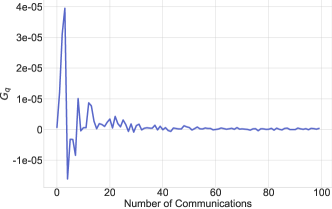
Figure 1: The error of quantization measured by Assumption 5 for FedCOMGATE with the MNIST dataset applied to a MLP model. We quantized updates $\boldsymbol{\Delta}_{j}$s from $32$ bits floating-point to $8$ bits integer.

The condition in Assumption 4 is not strict and only ensures that the local stochastic gradients are unbiased estimators of local gradients with bounded variance. Regarding Assumption 5, for the case of no compression, $Q(\boldsymbol{x})=\boldsymbol{x}$, the compression error becomes naturally $G_{q}=0$. We highlight that this assumption is only needed in the heterogeneous setting, and since both of the terms in the argument of expectation depend on the quantization, this assumption can be seen as a weaker version of the gradient diversity assumptions in the convergence analysis of heterogeneous settings. To show how this assumption holds in practice, we run an experiment on the MNIST dataset using FedCOMGATE algorithm with quantizing gradients from $32$ bits floating-point to $8$ bits integer. In Figure 1 we plot changes in $G_{q}$ quantity through this experiment. It shows that $G_{q}$ is decreasing as we proceed with the training, simply because the $\ell_{2}$-norm of the updated vector is going to zero. Note that the quantity of $G_{q}$ could be even negative as illustrated in Figure 1. For more details on the experiment see Section 6.

	Objective function
Reference	Nonconvex	PL/Strongly Convex	General Convex
SCAFFOLD[22]	$R=O\left(\frac{1}{\epsilon}\right)$ $\tau=O\left(\frac{1}{m\epsilon}\right)$	$R={O\left(\kappa\log\left(\frac{1}{\epsilon}\right)\right)}$ $\tau={O\left(\frac{1}{m\epsilon}\right)}$	$R={O\left(\frac{1}{\epsilon}\right)}$ $\tau={O\left(\frac{1}{m\epsilon}\right)}$
Local-SGD[23]	$-$	$-$	$R={O\left(\frac{1}{\epsilon^{1.5}}\right)}$ $\tau={O\left(\frac{1}{m\epsilon^{0.5}}\right)}$
VRL-SGD[30]	$R={O\left(\frac{m}{\epsilon}\right)}$ $\tau={O\left(\frac{1}{m^{2}\epsilon}\right)}$	$-$	$-$
Theorem 5.2	$\boldsymbol{R=O\left(\frac{1}{\epsilon}\right)}$ $\boldsymbol{\tau=O\left(\frac{1}{m\epsilon}\right)}$	$\boldsymbol{R=O\left(\kappa\log\left(\frac{1}{\epsilon}\right)\right)}$ $\boldsymbol{\tau=O\left(\frac{1}{m\epsilon}\right)}$	$\boldsymbol{R=O\left(\frac{1}{\epsilon}\log\left(\frac{1}{\epsilon}\right)\right)}$ $\boldsymbol{\tau=O\left(\frac{1}{m\epsilon^{2}}\right)}$

Table 6: Comparison of FedCOMGATE with results that use periodic averaging but do not utilize compression, i.e., $q=0$, in the heterogeneous setting. While SCAFFOLD [22] requires to communicate $2$ vectors to the server in the uplink, other algorithms only communicate $1$ vector.

Next, we present our main theoretical results for the FedCOMGATE method in the heterogeneous setting.

Theorem 5.2.

Consider FedCOMGATE in Algorithm 2. If Assumptions 1, 2, 4 and 5 hold, then even for the case the local data distribution of users are different (heterogeneous setting) we have

• Non-convex: By choosing stepsizes as $\eta=\frac{1}{L\gamma}\sqrt{\frac{m}{R\tau\left(q+1\right)}}$ and $\gamma\geq m$, we obtain that the iterates satsify $\frac{1}{R}\sum_{r=0}^{R-1}\left\|\nabla f({\boldsymbol{w}}^{(r)})\right\|_{2}^{2}\leq\epsilon$ if we set $R=O\left(\frac{q+1}{\epsilon}\right)$ and $\tau=O\left(\frac{1}{m\epsilon}\right)$.

• Strongly convex or PL: By choosing stepsizes as $\eta=\frac{1}{2L\left(\frac{q}{m}+1\right)\tau\gamma}$ and ${\gamma\geq\sqrt{m\tau}}$, we obtain that the iterates satisfy $\mathbb{E}\Big{[}f({\boldsymbol{w}}^{(R)})-f({\boldsymbol{w}}^{(*)})\Big{]}\leq\epsilon$ if we set $R=O\left(\left(q+1\right)\kappa\log\left(\frac{1}{\epsilon}\right)\right)$ and $\tau=O\left(\frac{1}{m\epsilon}\right)$.

• Convex: By choosing stepsizes as $\eta=\frac{1}{2L\left(q+1\right)\tau\gamma}$ and ${\gamma\geq\sqrt{m\tau}}$, we obtain that the iterates satisfy $\mathbb{E}\Big{[}f({\boldsymbol{w}}^{(R)})-f({\boldsymbol{w}}^{(*)})\Big{]}\leq\epsilon$ if we set $R=O\left(\frac{L\left(1+q\right)}{\epsilon}\log\left(\frac{1}{\epsilon}\right)\right)$ and $\tau=O\left(\frac{1}{m\epsilon^{2}}\right)$.

The implications of Theorem 5.2 are similar to the ones for Theorem 5.1. Yet, unlike the homogeneous setting, the compression variance $q$ does not scale down by a factor of $1/m$. We emphasize that similar to the homogeneous case, in all three cases, the dependency of $R$ on $\epsilon$ matches the number of required update for solving the problem in centralized fashion.

Remark 5.

To show the tightness of our result for FedCOMGATE, we also compare its complexity bounds with other schemes without compression, $q=0$, for heterogeneous settings, summarized in Table 6. As it can be observed in all settings, the bound for FedCOMGATE without compression (FedGATE) matches the best-known complexity bounds for these settings (upto a log factor).

Remark 6.

We highlight that since we do not need to communicate control variate in uplink, the communication cost of our algorithm is half of the corresponding cost in SCAFFOLD. Yet, for downlink communication, similar to SCAFFOLD our communication cost is doubled compared to FedAvg due to gradient tracking. However, we emphasize that in general communication cost of broadcasting a message is much cheaper than uplink communication.

6 Experiments

In this section, we empirically validate the performance of proposed algorithms. We compare our methods with FedAvg [37], its quantized version, FedPAQ [41], and SCAFFOLD [22] for heterogeneous federated learning. In addition, we present a variant of our algorithm without compression dubbed as FedGATE. The details of FedGATE is described in Algorithm 3 in Appendix B.1. Also, a variant of our algorithm with client sampling is presented in Algorithm 4 in Appendix B.1. In addition to what is presented here, in Appendix B.2, we explore the effects of client sampling, local computation, and sparsification on the convergence of our proposed algorithms.

Setup.

We implement our algorithms on the Distributed library of PyTorch [39], using Message Passing Interface (MPI), in order to simulate the real-world collaborative learning scenarios such as the one in federated learning. We run the experiments on a HPC cluster with $3$ Intel Xeon E5-2695 CPUs, each of which with $28$ processes. For this experiment we use four main datasets: MNIST [1], CIFAR10 [26], Fashion MNIST [59] and EMNIST [9]. For each experiment, we have $100$ devices communicating with the server. Each experiment runs for $100$ rounds of communication between clients and the server, and we report the global model loss on the training data averaged over all clients and the test accuracy over the global model. For MNIST and Fashion MNIST we use an MLP model with two hidden layers, each with $200$ neurons with ReLU activations. For the CIFAR10 dataset, we use the same MLP model, each layer with $500$ neurons. For the learning rate, we use a decreasing scheme similar to what is suggested in [7], where after each iteration the learning rate decreases $1\%$. Then, each experiment’s initial learning rate is tuned to achieve the best performance.

Homogeneous data distribution.

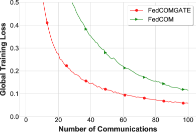
The FedCOM algorithm is best suited for the homogeneous case, while in the heterogeneous setting it suffers from a residual error. That is why we use gradient tracking in the FedCOMGATE algorithm. This error can be seen in Figure 3 for MNIST data, where in Figure 2(a) data is distributed homogeneously among devices, and in Figure 2(b) each device has access to only 2 classes in the dataset. The results indicate that we need gradient tracking in FedCOMGATE to deal with heterogeneity.

(a) Homogeneous

(b) Heterogeneous

Figure 2: Comparing Algorithm 1 and Algorithm 2 for homogeneous and heterogeneous data distributions of the MNIST dataset. In heterogeneous distribution, FedCOM suffers from a residual error.

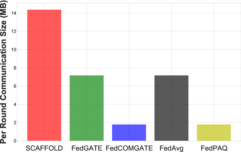
Figure 3: Communication cost at each round for the CIFAR10 dataset with a $2$-layer MLP.

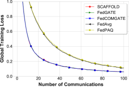
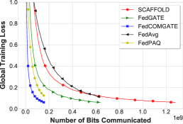
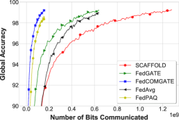
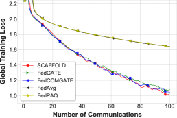
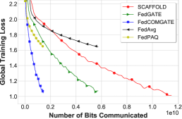
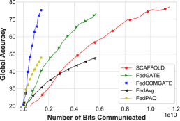
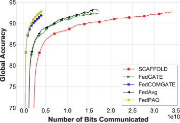
Figure 4: Comparing FedCOMGATE and FedGATE with FedAvg [37], FedPAQ [41], and SCAFFOLD [22] on the MNIST (first row) and the CIFAR10 (second row) datasets. Both FedCOMGATE and FedGATE outperform other algorithms in terms of communication size between clients and the server and convergence rate.

Heterogeneous data distribution.

To generate heterogeneous data that resembles a real federated learning setup, we will follow a similar approach as in [37]. In this regard, we will distribute the data among clients in a way that each client only has data from two classes, which is highly heterogeneous. The idea behind FedCOMGATE is similar to the one in SCAFFOLD, except in FedCOMGATE we only have one control variable that gets updated using normal updates in FedAvg. In contrast, SCAFFOLD has two control variables and requires to update the global model and server control variable at each round. Hence, each client in SCAFFOLD communicates at least twice the size as FedCOMGATE with the server at each round, when we do not use any compression. With compression, say $4\times$ quantization, we can substantially reduce the communication cost, say $8\times$, with respect to SCAFFOLD, while preserving the same convergence rate. To compare their communication cost, in Figure 3 we show the size of variables each client in each algorithm communicates with the server (for the uplink only, since the broadcasting or downlink time is negligible compared to the gathering) for the CIFAR10 dataset with an MLP model that has $2$ hidden layers, each with $500$ neurons. For FedCOMGATE and FedPAQ we quantize the updates from $32$ bits floating-point to $8$ bits integer.

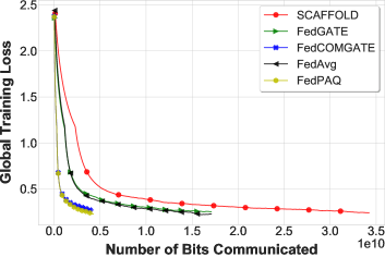
To show the effect of this communication size on the real-time convergence of each algorithm, we run each of them on the MNIST and the CIFAR10 datasets with MLP models as described before. The data is distributed heterogeneously among clients, where each one has access to only $2$ classes. Figure 4 shows the global model loss on training data on each communication round. FedAvg and FedPAQ are very close to each other on eacc, whereas FedCOMGATE, its normal version without compression FedGATE, and SCAFFOLD are performing similarly based on communication rounds. Figure 4 shows this loss based on the average number of bits communicated between each client and the server during the uplink. Also, Figure 4 shows the test accuracy based on this number of communicated bits. Both figures clearly demonstrate the effectiveness of proposed algorithms. Especially, the FedCOMGATE algorithm superbly outperforms other algorithms where the model size is relatively large.

EMNIST dataset

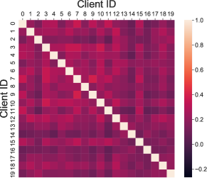
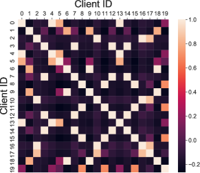
In addition to the results for the MNIST and CIFAR10 datasets we present the results of applying different algorithms on EMNIST [9] dataset. This dataset, similar to the MNIST dataset, contains images of characters in $28\times 28$ size. The difference here is that the dataset is separated based on the author of images, hence, the distribution each image is coming from is different for different nodes. In this experiment, we use data from $1000$ authors in the EMNIST dataset, and set the sampling ratio $k=0.1$. Also, we tune the learning rate to the fixed value of $0.01$ for all the algorithms. The model, similar to the MNIST case, is a 2-layer MLP with 200 neurons for each hidden layer and ReLU activations. Figure 5 shows the results of this experiment for the training loss and testing accuracy based on the size of communication. It can be inferred that FedCOMGATE and FedPAQ both have the fastest convergence based on the communication size, and accordingly, wall-clock time. The reason that the final convergence rate is the same for all algorithms is that similar to Figure 2(a), this dataset is close to the homogeneous setting. To show that, and to compare it to the heterogeneous datatset we created using the MNIST dataset, we run a test on $20$ different clients of this dataset and the heterogeneous MNIST dataset ($2$ classes data per client). We give all the clients the same model and perform a full batch gradient computation over that model. Then, we compute the cosine similarity of this gradients using:

$$d_{ij}=\frac{\mathbf{g}_{i}^{\top}\mathbf{g}_{j}}{\left\lVert\mathbf{g}_{i}\right\rVert\cdot\left\lVert\mathbf{g}_{j}\right\rVert}.$$ (7)

Figure 6 shows the heatmap of these correlations among clients for two datasets. As it can be seen, in the EMNIST dataset, each client’s data homogeneously correlates with all other clients’. However, in the MNIST dataset (with $2$ classes data per client), each client has high correlation with at most $4$ clients and not correlated or has a negative correlation with other clients’ data. This shows that the level of heterogeneity in the EMNIST dataset is much lower than that of in the MNIST dataset, and hence, the result in the Figure 5 are in line with our theoretical findings for the gradient tracking technique.

Figure 5: Comparing the performance of different algorithms on the EMNIST dataset, using $1000$ clients’ data on a 2-layer MLP model. FedCOMGATE and FedPAQ have the fastest convergence in time.

(a) EMNIST dataset

(b) MNIST dataset

Figure 6: Cosine similarity between full-gradients of different clients on the same model on EMNIST dataset and the heterogeneous MNIST (with $2$ classes per client) dataset. In the EMNIST dataset each client has a homogeneous correlation with other clients, while the MNIST dataset is highly heterogeneous.

7 Conclusion

In this paper we introduced a set of algorithms for federated learning which lower the communication overhead by periodic averaging and exchanging compressed signals. We considered two separate settings: (i) homogeneous setting in which all the probability distributions and loss functions are identical; and (ii) heterogeneous setting wherein the users’ distributions and loss functions could be different. For both cases, we showed that our proposed methods both theoretically and numerically require less communication rounds between server and users compared to state-of-the-art federated algorithms that use compression.

Appendix A Additional Related Work

In this section, we summarize and discuss additional related work. We separate the related work into two broad categories below.

Local computation with periodic communication.

An elegant idea to reduce the number of communications in vanilla synchronous SGD is to perform averaging periodically instead of averaging models in all clients at every iteration [62], also known as local SGD. The seminal work of [48] was among the first to analyze the convergence of local SGD in the homogeneous setting and demonstrated that the number of communication rounds can be significantly reduced for smooth and strongly convex objectives while achieving linear speedup. This result is further improved in follow up studies [13, 23, 53, 50, 61, 14]. In [53], the error-runtime trade-off of local SGD is analyzed and it has been shown that it can also alleviate the synchronization delay caused by slow workers. From a practical viewpoint, few recent efforts explored adaptive communication strategies to communicate more frequently early in the process [13, 32, 44].

The analysis of local SGD in the heterogeneous setting, also known as federated averaging (FedAvg) [37], has seen a resurgence of interest very recently. While it is still an active research area [57], a few number of recent studies made efforts to understand the convergence of local SGD in a heterogeneous setting [64, 15, 22, 25, 28, 23]. Also, the personalization of local models for a better generalization in a heterogeneous setting is of great importance from both theoretical and practical point of view [47, 10, 11, 36, 31].

Distributed optimization with compressed communication.

Another parallel direction of research has focused on reducing the size of communication by compressing the communicated messages. In quantization based methods, e.g. [45, 34, 50, 5], a quantization operator is applied before transmitting the gradient to server. A gradient acceleration approach with compression is proposed in [29]. In heterogeneous data distribution, [19] proposed the use of sign based SGD algorithms and [41] employed a quantization scheme in FedAvg with provable guarantees. In sparsification based methods, the idea is to transmit a smaller gradient vector by keeping only very few coordinates of local stochastic gradients, e.g., most significant entries [2, 35]. For these methods, theoretical guarantees have been provided in a few recent efforts [4, 52, 58, 49]. Note that, most of these studies rely on an error compensation technique as we employ in our experiments. We note that sketching methods are also employed to reduce the number of communication in [18].

The aforementioned studies mostly fall into the centralized distribution optimization. Recently a few attempts are made to explore the compression schema in a decentralized setting where each device shares compressed messages with direct neighbors over the underlying communication network  [42, 43, 46, 24]. Another interesting direction for the purpose of reducing the communication complexity is to exploit the sparsity of communication network as explored in [25, 54, 15].

Finally, more thorough related works that study federated learning from different perspectives can be found in [20] and [27].

Appendix B Further Experimental Studies and Results

In this section, we present additional experimental results, as well as details, that will further showcase the efficacy of the proposed algorithms in the paper. First, we should elaborate on the algorithms we used in Section 6, but due to lack of space we did not describe in the main body. In addition, we introduce a version of Algorithm 2 without compression, and its version with sampling of clients.

B.1 Variations of Algorithm 2

In this section we describe the details of variants of Algorithm 2 that are used in experiments.

Inputs: Number of communication rounds $R$, number of local updates $\tau$, learning rates $\gamma$ and $\eta$, initial global model $\boldsymbol{w}^{(0)}$, initial gradient tracking $\mathbf{\delta}_{j}^{(0)}=\boldsymbol{0},\;\forall j\in[m]$

[5pt]

for $r=0,\ldots,R-1$ do

       for each client $j\in[m]$ do in parallel

             Set $\boldsymbol{w}_{j}^{(0,r)}={\boldsymbol{w}}^{(r)}$

             for  $c=0,\ldots,\tau-1$ do

                   Set $\tilde{\boldsymbol{d}}^{(c,r)}_{j}=\tilde{\mathbf{g}}_{j}^{(c,r)}-\delta_{j}^{(r)}$ where $\tilde{\mathbf{g}}_{j}^{(c,r)}\triangleq\nabla f_{j}(\boldsymbol{w}^{(c,r)}_{j};\mathcal{Z}_{j}^{(c,r)})$

                   $\boldsymbol{w}^{(c+1,r)}_{j}=\boldsymbol{w}^{(c,r)}_{j}-\eta\leavevmode\nobreak\ \tilde{\boldsymbol{d}}^{(c,r)}_{j}$

             end for

            Device sends $\boldsymbol{u}_{j}^{(r)}={\boldsymbol{w}^{(r)}-\boldsymbol{w}^{(\tau,r)}_{j}}$ back to the server and gets $\boldsymbol{u}^{(r)}$

             Device computes $\bar{\boldsymbol{w}}^{(r)}=\boldsymbol{w}^{(r)}-\boldsymbol{u}^{(r)}$

             Device updates $\delta_{j}^{(r+1)}=\delta_{j}^{(r)}+\frac{1}{\eta\tau}\left(\bar{\boldsymbol{w}}^{(r)}-\boldsymbol{w}_{j}^{(\tau,r)}\right)$

             Device updates server model $\boldsymbol{w}^{(r+1)}=\boldsymbol{w}^{(r)}-\gamma\boldsymbol{u}^{(r)}$

              // Option I

            

            

       end forpar

      Server computes $\boldsymbol{u}^{(r)}=\frac{1}{m}\sum_{j=1}^{m}\boldsymbol{u}_{j}^{(r)}$ and broadcasts back to clients

       Server updates $\boldsymbol{w}^{(r+1)}=\boldsymbol{w}^{(r)}-\gamma\boldsymbol{u}^{(r)}$

       Server broadcasts ${\boldsymbol{w}}^{(r+1)}$ to all devices

        // Option II

      

end for

Algorithm 3 FedGATE($R,\tau,\eta,\gamma$) Federated Averaging with Local Gradient Tracking

Without compression.

In this part, we first elaborate on a variant of Algorithm 2 without any compression involved, which we call it Federated Averaging with Local Gradient Tracking, FedGATE. Algorithm 3 describes the steps of FedGATE, which involves a local gradient tracking step. This algorithm is similar to the SCAFFOLD [22], however, the main difference is that we do not use any server control variate. In fact, FedGATE, as well as FedCOMGATE, are implicitly controlling the variance of the server model by controlling its subsidiaries’ variances in local models. Therefore, there is no need to have another variable for this purpose, which can help us to greatly reduce the communication size, to half of what SCAFFOLD is using. Hence, even in the simple algorithm of FedGATE, we can gain the same convergence rate as SCAFFOLD, while enjoying the $2\times$ speedup in the communication. Note that, since the communication time of broadcasting from server to clients (or downlink communication) is negligible compared to gathering from clients to the server (or uplink communication), the overall communication complexity of this algorithm is close to FedAvg, and half of the SCAFFOLD, as it is depicted in Figure 3. Also, the communication complexity of FedCOMGATE is close to that of FedPAQ [41].

The common approach in federated learning without sampling for FedGATE and FedCOMGATE would be similar to Option II in Algorithm 3, where the server updates its model and broadcasts it to clients. This approach has one extra downlink step, that is negligible compared to the uplink steps, as it was mentioned before. However, when there is no sampling of the clients, we can avoid this extra downlink by using the Option I, where each local device keeps track of the server model and updates it based on what it gets for updating the gradient tracking variable. In practice, when sampling is not involved, we use Option I. In Section 6, we compare the performance of FedGATE and SCAFFOLD.

User sampling.

One important aspect of federated learning is the sampling of clients since they might not be available all the time. Also, sampling clients can further reduce the per round communication complexity by aggregating information from a subset of clients instead of all clients. Hence, in Algorithm 4, we incorporate the sampling mechanism into our proposed FedCOMGATE algorithm. Based on this algorithm, at each communication round, the server selects a subset of clients $\mathcal{S}^{(r)}\subseteq[m]$, and sends the global server model only to selected devices in $\mathcal{S}^{(r)}$. The remaining steps of the algorithm are similar to Algorithm 2. In Section 6, we also study the effect of user sampling on the performance of FedGATE, FedCOMGATE, and other state-of-the-art methods for federated learning.

Inputs: Number of communication rounds $R$, number of local updates $\tau$, learning rates $\gamma$ and $\eta$, initial global model $\boldsymbol{w}^{(0)}$, participation ratio of clients $k\in(0,1]$, initial gradient tracking $\mathbf{\delta}_{j}^{(0)}=\boldsymbol{0},\;\forall j\in[m]$

[2pt] for $r=0,\ldots,R-1$ do

       Sever selects a subset of devices $\mathcal{S}^{(r)}\subseteq[m]$, with the size $\lfloor km\rfloor$

       Server broadcasts ${w}^{(r)}$ to the selected devices $j\in\mathcal{S}^{(r)}$

      [3pt] for each client $j\in\mathcal{S}^{(r)}$ do in parallel

             Set $\boldsymbol{w}_{j}^{(0,r)}={\boldsymbol{w}}^{(r)}$

             for  $c=0,\ldots,\tau-1$ do

                   Set $\tilde{\boldsymbol{d}}^{(c,r)}_{j,q}=\tilde{\mathbf{g}}_{j}^{(c,r)}-\delta_{j}^{(r)}$ where $\tilde{\mathbf{g}}_{j}^{(c,r)}\triangleq\nabla f_{j}(\boldsymbol{w}^{(c,r)}_{j};\mathcal{Z}_{j}^{(c,r)})$

                   $\boldsymbol{w}^{(c+1,r)}_{j}=\boldsymbol{w}^{(c,r)}_{j}-\eta\leavevmode\nobreak\ \tilde{\boldsymbol{d}}^{(c,r)}_{j,q}$

             end for

            Device sends $\boldsymbol{\Delta}_{j,q}^{(r)}=Q(({\boldsymbol{w}^{(r)}-\boldsymbol{w}^{(\tau,r)}_{j}})/\eta)$ back to the server and gets $\boldsymbol{\Delta}_{q}^{(r)}$

             Device updates $\delta_{j}^{(r+1)}=\delta_{j}^{(r)}+\frac{1}{\tau}(\boldsymbol{\Delta}_{j,q}^{(r)}-\boldsymbol{\Delta}_{q}^{(r)})$

       end forpar

      Server computes $\boldsymbol{\Delta}_{q}^{(r)}=\frac{1}{m}\sum_{j=1}^{m}\boldsymbol{\Delta}_{j,q}^{(r)}$ and broadcasts back to devices $j\in\mathcal{S}^{(r)}$

       Server computes $\boldsymbol{w}^{(r+1)}=\boldsymbol{w}^{(r)}-\eta\gamma\boldsymbol{\Delta}_{q}^{(r)}$

      

end for

Algorithm 4 FedCOMGATE($R,\tau,\eta,\gamma,k$), FedCOMGATE algorithm with sampling of clients

B.2 Additional Experiments

Sampling clients

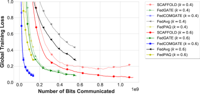
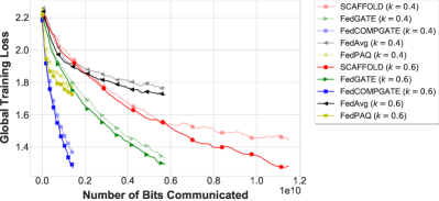
In this section we assume that only $k\in(0,1]$ portion of the users in the networks are active and exchange information with the server at each round. Indeed, a lower value of $k$ implies that less nodes are active at each round and therefore the communication overhead is lower. However, it could possibly lead to a slower convergence rate and extra communications rounds to achieve a specific accuracy. We formally study the effect of $k$ on the convergence of FedCOMGATE and its version without compression FedGATE and compare their performance with other federated methods with and without compression in Figure 7. As it can be inferred, when we decrease the $k$ or the participation rate, generally, the performance of the model degrades with the same number of communication rounds. However, the amount of degradation might vary among different algorithms. As it is depicted in Figure 7, the proposed FedCOMGATE algorithm and its unquantized version, FedGATE, are quite robust against decreasing the participation rate between clients with respect to other algorithms such as SCAFFOLD and FedPAQ.

An important difference between algorithms proposed in this work (such as FedCOMGATE) and SCAFFOLD is in their performance when not all clients are active at each round of communication. Since in SCAFFOLD gradient tracking needs to be performed both locally and globally at each round of communication, its performance could highly depend on the availability of control variate in all devices. This can lead to poor performance for SCAFFOLD when the rate of participation of clients at each round is low (as illustrated in Figure 7). This could be due to stale local control variate and new global control variate that degrade the performance of the algorithm. On the other hand, in our proposed algorithms, the gradient tracking parameter is only performed locally, and hence, the drop in the performance is much smaller than SCAFFOLD. Therefore, we think this property makes our proposed algorithms suitable for the cross-device scenarios as well as cross-silo ones, whereas SCAFFOLD is more suitable for cross-silo scenarios, and not cross-device ones.

(a) MNIST Dataset

(b) CIFAR10 Dataset

Figure 7: Comparing the effect of sampling on different algorithms. We use two datasets: the MNIST and the CIFAR10 datasets. We use an MLP with 2 layers for all the datasets, with $200$ neurons per layer for the MNIST, and $500$ neurons per layer for the CIFAR10. FedGATE and FedCOMGATE seem to be more robust against client sampling.

(a) MNIST Dataset

(b) Fashion MNIST Dataset

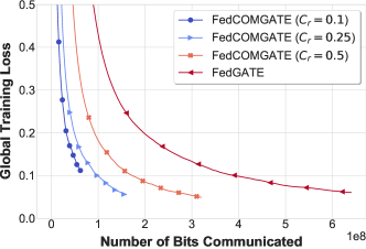
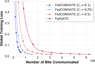
Figure 8: The effect of sparsification with memory on the FedCOMGATE algorithm used for the training of the MNIST and the Fashion MNIST datasets. We can achieve almost similar results as the algorithm without compression (FedGATE) with some compression rates. Decreasing the size of communication will speed up the training, in the cost of increasing a residual error as it is evident for the case with $C_{r}=0.1$.

Compression via sparsification.

Another approach to compress the gradient updates is sparsification. This method has been vastly used in distributed training of machine learning models [49, 2, 55]. Using a simple sparsification by choosing random elements or $top_{k}$ elements, some information will be lost in aggregating gradients, and consequently, the quality of the model will be degraded. To overcome this problem, an elegant idea is proposed in [48] to use memory for tracking the history of entries and avoid the accumulation of compression errors. Similarly, we will employ a memory of aggregating gradients in order to compensate for the loss of information from sparsification. This is in addition to the local gradient tracking we incorporated in FedCOMGATE, however, despite the server control variate in SCAFFOLD, this memory is updated locally and is not required to be communicated to the server. We denote the memory in each client $j$ at round $r$ with $\boldsymbol{\nu}_{j}^{(r)}$. Thus, in Algorithm 2, we first need to compress the gradients added by the memory, using the $top_{k}$ operator as:

$$\boldsymbol{\Delta}_{j,s}^{(r)}=top_{k}\left\{\left(\boldsymbol{w}^{(r)}-\boldsymbol{w}^{(\tau,r)}_{j}\right)+\boldsymbol{\nu}_{j}^{(r)}\right\}$$ (8)

Then, we will send this to the server for aggregation, where the server decompresses them, takes the average, and sends $\boldsymbol{\Delta}^{(r)}$ back to the clients. Each client updates its gradient tracking parameter as in Algorithm 2. Also, in this case, we need to update the memory parameter as:

$$\boldsymbol{\nu}_{j}^{(r+1)}=\boldsymbol{\nu}_{j}^{(r)}+\frac{1}{m}\left(\boldsymbol{w}^{(r)}-\boldsymbol{w}^{(\tau,r)}_{j}\right)-\boldsymbol{\Delta}^{(r)},$$ (9)

where it keeps track of what was not captured by the aggregation using the sparsified gradients. Note that, unlike the quantized FedCOMGATE, in this approach, we cannot compress the downlink gradient broadcasting. However, since the cost of broadcasting is much lower than the uplink communication, this is negligible, especially in lower compression rates compared to quantized FedCOMGATE.

To show how the FedCOMGATE using sparsification with memory works in practice we will apply it to MNIST and Fashion MNIST datasets. Both of them are applied to an MLP model with two hidden layers, each with $200$ neurons. For this experiment, we use the compression ratio parameter of $C_{r}$, which is the ratio between the size of communication in the compressed and without compression versions. Figure 8 shows the result of this algorithm by changing the compression rate. As it was observed by [49], in some compression rates we can have similar or slightly better results than the without compression distributed SGD solution (here FedGATE), due to the use of memory. However, to gain more from the speedup and decreasing the compression rate, we will incur a residual error, as it can be seen in the results for the compression rate of $0.1$.

(a) Effect of quantization noise $q$

(b) Effect of local computation $\tau$

Figure 9: Investigating the effects of quantization noise and local computations on the convergence rate. We run the experiments on the MNIST dataset with a similar MLP model as before. In (a), we increase the noise of quantization by increasing the range of noise added to the zero-point of the quantizer operator. Increasing $q$ can degrade the convergence rate of the model. On the other hand, in (b), with the same level of quantization noise, we can increase the number of local computations $\tau$ to diminish the effects of quantization.

Effect of local computations.

Finally, we will show the effect of noise in quantization, characterized as $q$ in the paper, on the convergence rate, and how to address it. As it can be inferred from our theoretical analysis, increasing the noise of quantization would degrade the convergence rate of the model. This pattern can be seen in Figure 9(a) for the MNIST dataset, where we add noise to quantized arrays by adding a random integer to the zero-point of the quantization operator. By increasing the range of this noise, we can see that the convergence is getting worse with the same number of local computations. On the other hand, based on our analysis, we know that increasing the number of local computations will compensate for the quantization noise, which helps us to achieve the same results with lower communication rounds. This pattern is depicted in Figure 9(b), where we keep the quantization noise constant and increase the number of local computations.

Appendix C Some Definitions and Notation

Before stating our proofs we first formally define Polyak-Łojasiewicz and strongly convex functions.

Assumption 6 (Polyak-Łojasiewicz).

A function $f(\boldsymbol{w})$ satisfies the Polyak-Łojasiewicz  condition with constant $\mu$ if $\frac{1}{2}\|\nabla f(\boldsymbol{w})\|_{2}^{2}\geq\mu\big{(}f(\boldsymbol{w})-f(\boldsymbol{w}^{*})\big{)},\>\forall\boldsymbol{w}\in\mathbb{R}^{d}$ with $\boldsymbol{w}^{*}$ is an optimal solution.

Assumption 7 ($\mu$-strong convexity).

A function $f$ is $\mu$-strongly convex if it satisfies $f(\boldsymbol{u})\geq f(\boldsymbol{v})+\left\langle\nabla{f}(\boldsymbol{v}),\boldsymbol{u}-\boldsymbol{v}\right\rangle+\frac{\mu}{2}\left\|\boldsymbol{u}-\boldsymbol{v}\right\|^{2}$, for all $\boldsymbol{u},\boldsymbol{v}\in\mathbb{R}^{d}$.

We also introduce some notation for the clarity in presentation of proofs. Recall that we use $\mathbf{g}_{i}={\nabla{f}_{i}(\boldsymbol{w})\triangleq\nabla{f}_{i}(\boldsymbol{w};\mathcal{S}_{i})}$ and $\tilde{\mathbf{g}}_{i}\triangleq\nabla{f}(\boldsymbol{w};\mathcal{Z}_{i})$ for ${1\leq i\leq m}$ to denote the full gradient and stochastic gradient at $i$th data shard, respectively, where $\mathcal{Z}_{i}\subseteq\mathcal{S}_{i}$ is a uniformly sampled mini-bath. The corresponding quantities evaluated at $i$th machine’s local solution at $t$th iteration of optimization $\boldsymbol{w}_{i}^{(t)}$ are denoted by $\mathbf{g}_{i}^{(t)}$ and $\tilde{\mathbf{g}}_{i}^{(t)}$, where we abuse the notation and use $t=r\tau+c$ to denote the $c$th local update at $r$th round, i.e. $(c,r)$. We also define the following notations

$$\boldsymbol{w}^{(t)} =\{\boldsymbol{w}^{(t)}_{1},\ldots,\boldsymbol{w}^{(t)}_{m}\},$$

$${\xi}^{(t)} =\{{\xi}^{(t)}_{1},\ldots,{\xi}^{(t)}_{m}\},$$

to denote the set of local solutions and sampled mini-batches at iteration $t$ at different machines, respectively. Finally, we use notation $\mathbb{E}[\cdot]$ to denote the conditional expectation $\mathbb{E}_{{\xi}^{(t)}|{\boldsymbol{w}}^{(t)}}[\cdot]$.

Appendix D Results for the Homogeneous Setting

In this section, we study the convergence properties of our FedCOM method presented in Algorithm 1. Before stating the proofs for FedCOM in the homogeneous setting, we first mention the following intermediate lemmas.

Lemma D.1.

Under Assumptions 2 and 3, we have the following bound:

$$\mathbb{E}_{{Q,\xi^{(r)}}}\Big{[}\|\tilde{\mathbf{g}}_{Q}^{(r)}\|^{2}\Big{]} =\mathbb{E}_{{\xi}^{(r)}}\mathbb{E}_{{Q}}\Big{[}\|\tilde{\mathbf{g}}_{Q}^{(r)}\|^{2}\Big{]}\leq\tau(q+1)\frac{1}{m}\sum_{j=1}^{m}\sum_{c=0}^{\tau-1}\|\mathbf{g}_{j}^{(c,r)}\|^{2}+\left(q+1\right)\frac{\tau\sigma^{2}}{m}$$ (10)

Proof.

$$\mathbb{E}_{{\xi^{(r)}|\boldsymbol{w}^{(r)}}}\mathbb{E}_{{Q}}\Big{[}\|\frac{1}{m}\sum_{j=1}^{m}Q\left(\sum_{c=0}^{\tau-1}\tilde{\mathbf{g}}^{(c,r)}_{j}\right)\|^{2}\Big{]}$$

$$=\mathbb{E}_{{\xi}^{(r)}}\left[\mathbb{E}_{{Q}}\Big{[}\|\frac{1}{m}\sum_{j=1}^{m}\underbrace{Q\left(\overbrace{\sum_{c=0}^{\tau-1}\tilde{\mathbf{g}}^{(c,r)}_{j}}^{\tilde{\mathbf{g}}_{j}^{(r)}}\right)}_{\tilde{\mathbf{g}}_{Qj}^{(r)}}\|^{2}\Big{]}\right]$$

$$\stackrel{{\scriptstyle\text{\char 192}}}{{=}}\mathbb{E}_{{\xi}^{(r)}}\left[\mathbb{E}_{{Q}}\left[\left[\|\frac{1}{m}\sum_{j=1}^{m}\tilde{\mathbf{g}}_{Qj}^{(r)}-\frac{1}{m}\sum_{j=1}^{m}\mathbb{E}_{{Q}}\left[\tilde{\mathbf{g}}_{Qj}^{(r)}\right]\|^{2}\right]+\|\mathbb{E}_{{Q}}\left[\frac{1}{m}\sum_{j=1}^{m}\tilde{\mathbf{g}}_{Qj}^{(r)}\right]\|^{2}\right]\right]$$

$$\stackrel{{\scriptstyle\text{\char 193}}}{{=}}\mathbb{E}_{{\xi}^{(r)}}\left[\mathbb{E}_{{Q}}\left[\frac{1}{m^{2}}\sum_{j=1}^{m}\left[\left\|\tilde{\mathbf{g}}_{Qj}^{(r)}-\tilde{\mathbf{g}}^{(r)}_{j}\right\|^{2}\right]\right]+\left\|\frac{1}{m}\sum_{j=1}^{m}\tilde{\mathbf{g}}_{j}^{(r)}\right\|^{2}\right]$$

$$\stackrel{{\scriptstyle\text{\char 194}}}{{\leq}}\mathbb{E}_{{\xi}^{(r)}}\left[\sum_{j=1}^{m}\frac{q}{m^{2}}\left\|\tilde{\mathbf{g}}_{j}^{(r)}\right\|^{2}+\left\|\frac{1}{m}\sum_{j=1}^{m}\tilde{\mathbf{g}}_{j}^{(r)}\right\|^{2}\right]$$

$$=\left[\sum_{j=1}^{m}\frac{q}{m^{2}}\left[\text{Var}\left(\tilde{\mathbf{g}}_{j}^{(r)}\right)+\left\|{\mathbf{g}}_{j}^{(r)}\right\|^{2}\right]+\left[\text{Var}\left(\frac{1}{m}\sum_{j=1}^{m}\tilde{\mathbf{g}}_{j}^{(r)}\right)+\left\|\frac{1}{m}\sum_{j=1}^{m}{\mathbf{g}}_{j}^{(r)}\right\|^{2}\right]\right]$$

$$=\sum_{j=1}^{m}\frac{q}{m^{2}}\left[\text{Var}\left(\tilde{\mathbf{g}}_{j}^{(r)}\right)+\left\|{\mathbf{g}}_{j}^{(r)}\right\|^{2}\right]+\left[\frac{1}{m^{2}}\sum_{j=1}^{m}\text{Var}\left(\tilde{\mathbf{g}}_{j}^{(r)}\right)+\left\|\frac{1}{m}\sum_{j=1}^{m}{\mathbf{g}}_{j}^{(r)}\right\|^{2}\right]$$

$$\leq\sum_{j=1}^{m}\frac{q}{m^{2}}\left[\text{Var}\left(\tilde{\mathbf{g}}_{j}^{(r)}\right)+\left\|{\mathbf{g}}_{j}^{(r)}\right\|^{2}\right]+\left[\frac{1}{m^{2}}\sum_{j=1}^{m}\text{Var}\left(\tilde{\mathbf{g}}_{j}^{(r)}\right)+\frac{1}{m}\sum_{j=1}^{m}\left\|{\mathbf{g}}_{j}^{(r)}\right\|^{2}\right]$$ (11)

where ➀ holds due to $\mathbb{E}\left[\left\|\mathbf{x}\right\|^{2}\right]=\text{Var}[\mathbf{x}]+\left\|\mathbb{E}[\mathbf{x}]\right\|^{2}$, ➁ is due to $\mathbb{E}_{{Q}}\left[\frac{1}{m}\sum_{j=1}^{m}\tilde{\mathbf{g}}_{Qj}^{(r)}\right]=\frac{1}{m}\sum_{j=1}^{m}\tilde{\mathbf{g}}_{j}^{(r)}$ and ➂ follows from Assumption 2.

Next we show that from Assumptions 4, we have

$$\mathbb{E}_{\xi^{(r)}}\left[\Big{[}\|{\tilde{\mathbf{g}}_{j}^{(r)}}-{\mathbf{g}_{j}^{(r)}}\|^{2}\Big{]}\right]\leq\tau\sigma^{2}$$ (12)

To do so, note that

$$\mathbb{E}_{\xi^{(r)}}\left[\left\|{\tilde{\mathbf{g}}_{j}^{(r)}}-{\mathbf{g}_{j}^{(r)}}\right\|^{2}\right] \stackrel{{\scriptstyle\text{\char 192}}}{{=}}\mathbb{E}_{\xi^{(r)}}\left[\left\|\sum_{c=0}^{\tau-1}\left[\tilde{\mathbf{g}}_{j}^{(c,r)}-\mathbf{g}_{j}^{(c,r)}\right]\right\|^{2}\right]$$

$${=}\text{Var}\left(\sum_{c=0}^{\tau-1}\tilde{\mathbf{g}}_{j}^{(c,r)}\right)$$

$$\stackrel{{\scriptstyle\text{\char 193}}}{{=}}\sum_{c=0}^{\tau-1}\text{Var}\left(\tilde{\mathbf{g}}_{j}^{(c,r)}\right)$$

$${=}\sum_{c=0}^{\tau-1}\mathbb{E}\left[\left\|\tilde{\mathbf{g}}_{j}^{(c,r)}-\mathbf{g}_{j}^{(c,r)}\right\|^{2}\right]$$

$$\stackrel{{\scriptstyle\text{\char 194}}}{{\leq}}\tau\sigma^{2}$$ (13)

where in ➀ we use the definition of ${\tilde{\mathbf{g}}}_{j}^{(r)}$ and ${{\mathbf{g}}}_{j}^{(r)}$, in ➁ we use the fact that mini-batches are chosen in i.i.d. manner at each local machine, and ➂ immediately follows from Assumptions 3.

Replacing $\mathbb{E}_{\xi^{(r)}}\left[\|{\tilde{\mathbf{g}}_{j}^{(r)}}-{\mathbf{g}_{j}^{(r)}}\|^{2}\right]$ in (11) by its upper bound in (12) implies that

$$\mathbb{E}_{{\xi^{(r)}|\boldsymbol{w}^{(r)}}}\mathbb{E}_{{Q}}\Big{[}\|\frac{1}{m}\sum_{j=1}^{m}Q\left(\sum_{c=0}^{\tau-1}\tilde{\mathbf{g}}^{(c,r)}_{j}\right)\|^{2}\Big{]}\leq\sum_{j=1}^{m}\frac{q}{m^{2}}\left[\tau\sigma^{2}+\left\|{\mathbf{g}}_{j}^{(r)}\right\|^{2}\right]+\left[\frac{1}{m^{2}}\sum_{j=1}^{m}\tau\sigma^{2}+\frac{1}{m}\sum_{j=1}^{m}\left\|{\mathbf{g}}_{j}^{(r)}\right\|^{2}\right]$$ (14)

Further note that we have

$$\left\|{\mathbf{g}}_{j}^{(r)}\right\|^{2} =\|\sum_{c=0}^{\tau-1}\mathbf{g}_{j}^{(c,r)}\|^{2}\stackrel{{\scriptstyle}}{{\leq}}\tau\sum_{c=0}^{\tau-1}\|\mathbf{g}_{j}^{(c,r)}\|^{2}$$ (15)

where the last inequality is due to $\left\|\sum_{j=1}^{n}\mathbf{a}_{i}\right\|^{2}\leq n\sum_{j=1}^{n}\left\|\mathbf{a}_{i}\right\|^{2}$, which together with (14) leads to the following bound:

$$\mathbb{E}_{{\xi^{(r)}|\boldsymbol{w}^{(r)}}}\mathbb{E}_{{Q}}\Big{[}\|\frac{1}{m}\sum_{j=1}^{m}Q\left(\sum_{c=0}^{\tau-1}\tilde{\mathbf{g}}^{(c,r)}_{j}\right)\|^{2}\Big{]}\leq\tau(\frac{q}{m}+1)\frac{1}{m}\sum_{j=1}^{m}\sum_{c=0}^{\tau-1}\|\mathbf{g}_{j}^{(c,r)}\|^{2}+\left(q+1\right)\frac{\tau\sigma^{2}}{m},$$ (16)

and the proof is complete. ∎

Lemma D.2.

Under Assumption 1, and according to the FedCOM algorithm the expected inner product between stochastic gradient and full batch gradient can be bounded with:

$$-\mathbb{E}\left[\left\langle\nabla f({\boldsymbol{w}}^{(r)}),{{\tilde{\mathbf{g}}}^{(r)}}\right\rangle\right] \leq\frac{1}{2}\eta\frac{1}{m}\sum_{j=1}^{m}\sum_{c=0}^{\tau-1}\left[-\|\nabla f({\boldsymbol{w}}^{(r)})\|_{2}^{2}-\|\nabla{f}(\boldsymbol{w}_{j}^{(c,r)})\|_{2}^{2}+L^{2}\|{\boldsymbol{w}}^{(r)}-\boldsymbol{w}_{j}^{(c,r)}\|_{2}^{2}\right]$$ (17)

Proof.

We have:

$$-\mathbb{E}_{\{{\xi}^{(t)}_{1},\ldots,{\xi}^{(t)}_{m}|{\boldsymbol{w}}^{(t)}_{1},\ldots,{\boldsymbol{w}}^{(t)}_{m}\}}\mathbb{E}_{Q}\left[\big{\langle}\nabla f({\boldsymbol{w}}^{(r)}),\tilde{\mathbf{g}}_{Q}^{(r)}\big{\rangle}\right]$$

$$=-\mathbb{E}_{\{{\xi}^{(t)}_{1},\ldots,{\xi}^{(t)}_{m}|{\boldsymbol{w}}^{(t)}_{1},\ldots,{\boldsymbol{w}}^{(t)}_{m}\}}\left[\left\langle\nabla f({\boldsymbol{w}}^{(r)}),\eta\frac{1}{m}\sum_{j=1}^{m}\sum_{c=0}^{\tau-1}\tilde{\mathbf{g}}_{j}^{(c,r)}\right\rangle\right]$$

$$=-\left\langle\nabla f({\boldsymbol{w}}^{(r)}),\eta\frac{1}{m}\sum_{j=1}^{m}\sum_{c=0}^{\tau-1}\mathbb{E}\left[\tilde{\mathbf{g}}_{j}^{(c,r)}\right]\right\rangle$$

$$=-\eta\sum_{c=0}^{\tau-1}\frac{1}{m}\sum_{j=1}^{m}\left\langle\nabla f({\boldsymbol{w}}^{(r)}),{\mathbf{g}}_{j}^{(c,r)}\right\rangle$$

$$\stackrel{{\scriptstyle\text{\char 192}}}{{=}}\frac{1}{2}\eta\sum_{c=0}^{\tau-1}\frac{1}{m}\sum_{j=1}^{m}\left[-\|\nabla f({\boldsymbol{w}}^{(r)})\|_{2}^{2}-\|{{\nabla{f}}}(\boldsymbol{w}_{j}^{(c,r)})\|_{2}^{2}+\|\nabla f({\boldsymbol{w}}^{(r)})-\nabla{f}(\boldsymbol{w}_{j}^{(c,r)})\|_{2}^{2}\right]$$

$$\stackrel{{\scriptstyle\text{\char 193}}}{{\leq}}\frac{1}{2}\eta\sum_{c=0}^{\tau-1}\frac{1}{m}\sum_{j=1}^{m}\left[-\|\nabla f({\boldsymbol{w}}^{(r)})\|_{2}^{2}-\|\nabla{f}(\boldsymbol{w}_{j}^{(c,r)})\|_{2}^{2}+L^{2}\|{\boldsymbol{w}}^{(r)}-\boldsymbol{w}_{j}^{(c,r)}\|_{2}^{2}\right]$$ (18)

where ➀ is due to $2\langle\mathbf{a},\mathbf{b}\rangle=\|\mathbf{a}\|^{2}+\|\mathbf{b}\|^{2}-\|\mathbf{a}-\mathbf{b}\|^{2}$, and ➁ follows from Assumption 1. ∎

The following lemma bounds the distance of local solutions from global solution at $r$th communication round.

Lemma D.3.

Under Assumptions 3 we have:

$$\mathbb{E}\left[\|{\boldsymbol{w}}^{(r)}-\boldsymbol{w}_{j}^{(c,r)}\|_{2}^{2}\right] \leq\eta^{2}\tau\sum_{c=0}^{\tau-1}\left\|{\mathbf{g}}_{j}^{(c,r)}\right\|_{2}^{2}+\eta^{2}\tau\sigma^{2}$$ (19)

Proof.

Note that

$$\mathbb{E}\left[\left\|{\boldsymbol{w}}^{(r)}-\boldsymbol{w}_{j}^{(c,r)}\right\|_{2}^{2}\right] =\mathbb{E}\left[\left\|{\boldsymbol{w}}^{(r)}-\left({\boldsymbol{w}}^{(r)}-\eta\sum_{k=0}^{c}\tilde{\mathbf{g}}_{j}^{(k,r)}\right)\right\|_{2}^{2}\right]$$

$$=\mathbb{E}\left[\left\|\eta\sum_{k=0}^{c}\tilde{\mathbf{g}}_{j}^{(k,r)}\right\|_{2}^{2}\right]$$

$$\stackrel{{\scriptstyle\text{\char 192}}}{{=}}\mathbb{E}\left[\left\|\eta\sum_{k=0}^{c}\left(\tilde{\mathbf{g}}_{j}^{(k,r)}-{\mathbf{g}}_{j}^{(k,r)}\right)\right\|_{2}^{2}\right]+\left[\left\|\eta\sum_{k=0}^{c}{\mathbf{g}}_{j}^{(k,r)}\right\|_{2}^{2}\right]$$

$$\stackrel{{\scriptstyle\text{\char 193}}}{{=}}\eta^{2}\sum_{k=0}^{c}\mathbb{E}\left[\left\|\left(\tilde{\mathbf{g}}_{j}^{(k,r)}-{\mathbf{g}}_{j}^{(k,r)}\right)\right\|_{2}^{2}\right]+\left(c+1\right)\eta^{2}\sum_{k=0}^{c}\left[\left\|{\mathbf{g}}_{j}^{(k,r)}\right\|_{2}^{2}\right]$$

$${\leq}\eta^{2}\sum_{k=0}^{\tau-1}\mathbb{E}\left[\left\|\left(\tilde{\mathbf{g}}_{j}^{(k,r)}-{\mathbf{g}}_{j}^{(k,r)}\right)\right\|_{2}^{2}\right]+\tau\eta^{2}\sum_{k=0}^{\tau-1}\left[\left\|{\mathbf{g}}_{j}^{(k,r)}\right\|_{2}^{2}\right]$$

$$\stackrel{{\scriptstyle\text{\char 194}}}{{\leq}}\eta^{2}\sum_{k=0}^{\tau-1}\sigma^{2}+\tau\eta^{2}\sum_{k=0}^{\tau-1}\left[\left\|{\mathbf{g}}_{j}^{(k,r)}\right\|_{2}^{2}\right]$$

$${=}\eta^{2}\tau\sigma^{2}+\eta^{2}\sum_{k=0}^{\tau-1}\tau\left\|{\mathbf{g}}_{j}^{(k,r)}\right\|_{2}^{2}$$ (20)

where ➀ comes from $\mathbb{E}\left[\mathbf{x}^{2}\right]=\text{Var}\left[\mathbf{x}\right]+\left[\mathbb{E}\left[\mathbf{x}\right]\right]^{2}$ and ➁ holds because $\text{Var}\left(\sum_{j=1}^{n}\mathbf{x}_{j}\right)=\sum_{j=1}^{n}\text{Var}\left(\mathbf{x}_{j}\right)$ for i.i.d. vectors $\mathbf{x}_{i}$ (and i.i.d. assumption comes from i.i.d. sampling), and finally ➂ follows from Assumption 3. ∎

D.1 Main result for the non-convex setting

Now we are ready to present our result for the homogeneous setting. We first state and prove the result for the general nonconvex objectives.

Theorem D.4 (Non-convex).

For FedCOM$(\tau,\eta,\gamma)$, for all $0\leq t\leq R\tau-1$, under Assumptions 1 to 3, if the learning rate satisfies

$$1\geq{\tau^{2}L^{2}\eta^{2}}+\left(\frac{q}{m}+1\right){\eta\gamma L}{\tau}$$ (21)

and all local model parameters are initialized at the same point ${\boldsymbol{w}}^{(0)}$, then the average-squared gradient after $\tau$ iterations is bounded as follows:

$$\frac{1}{R}\sum_{r=0}^{R-1}\left\|\nabla f({\boldsymbol{w}}^{(r)})\right\|_{2}^{2}\leq\frac{2\left(f(\boldsymbol{w}^{(0)})-f(\boldsymbol{w}^{(*)})\right)}{\eta\gamma\tau R}+\frac{L\eta\gamma{\left(q+1\right)}}{m}\sigma^{2}+{L^{2}\eta^{2}\tau}\sigma^{2}$$ (22)

where $\boldsymbol{w}^{(*)}$ is the global optimal solution with function value $f(\boldsymbol{w}^{(*)})$.

Proof.

Before proceeding to the proof of Theorem D.4, we would like to highlight that

$$\boldsymbol{w}^{(r)}-\leavevmode\nobreak\ {\boldsymbol{w}}_{j}^{(\tau,r)}=\eta\sum_{c=0}^{\tau-1}\tilde{\mathbf{g}}_{j}^{(c,r)}.$$ (23)

From the updating rule of Algorithm 1 we have

$${\boldsymbol{w}}^{(r+1)}=\boldsymbol{w}^{(r)}-\gamma\eta\left(\frac{1}{m}\sum_{j=1}^{m}Q\Big{(}\sum_{c=0,r}^{\tau-1}\tilde{\mathbf{g}}_{j}^{(c,r)}\Big{)}\right)=\boldsymbol{w}^{(r)}-\gamma\left[\frac{\eta}{m}\sum_{j=1}^{m}Q\left(\sum_{c=0}^{\tau-1}\tilde{\mathbf{g}}_{j}^{(c,r)}\right)\right]$$ (24)

In what follows, we use the following notation to denote the stochastic gradient used to update the global model at $r$th communication round

$$\tilde{\mathbf{g}}_{Q}^{(r)}\triangleq\frac{\eta}{m}\sum_{j=1}^{m}{Q}\left(\frac{\boldsymbol{w}^{(r)}-\leavevmode\nobreak\ {\boldsymbol{w}}_{j}^{(\tau,r)}}{\eta}\right)=\frac{\eta}{m}\sum_{j=1}^{m}{Q}\left(\sum_{c=0}^{\tau-1}\tilde{\mathbf{g}}_{j}^{(c,r)}\right).$$

and notice that $\boldsymbol{w}^{(r)}=\boldsymbol{w}^{(r-1)}-\gamma\tilde{\mathbf{g}}^{(r)}$.

Then using the Assumption 2 we have:

$$\mathbb{E}_{Q}\left[\tilde{\mathbf{g}}_{Q}^{(r)}\right]=\frac{1}{m}\sum_{j=1}\left[-\eta\mathbb{E}_{Q}\left[Q\left(\sum_{c=0}^{\tau-1}\tilde{\mathbf{g}}_{j}^{(c,r)}\right)\right]\right]=\frac{1}{m}\sum_{j=1}\left[-\eta\left(\sum_{c=0}^{\tau-1}\tilde{\mathbf{g}}_{j}^{(c,r)}\right)\right]\triangleq\tilde{\mathbf{g}}^{(r)}$$ (25)

From the $L$-smoothness gradient assumption on global objective, by using $\tilde{\mathbf{g}}^{(r)}$ in inequality (23) we have:

$$f({\boldsymbol{w}}^{(r+1)})-f({\boldsymbol{w}}^{(r)})\leq-\gamma\big{\langle}\nabla f({\boldsymbol{w}}^{(r)}),\tilde{\mathbf{g}}^{(r)}\big{\rangle}+\frac{\gamma^{2}L}{2}\|\tilde{\mathbf{g}}^{(r)}\|^{2}$$ (26)

By taking expectation on both sides of above inequality over sampling, we get:

$$\mathbb{E}\left[\mathbb{E}_{Q}\Big{[}f({\boldsymbol{w}}^{(r+1)})-f({\boldsymbol{w}}^{(r)})\Big{]}\right] \leq-\gamma\mathbb{E}\left[\mathbb{E}_{Q}\left[\big{\langle}\nabla f({\boldsymbol{w}}^{(r)}),\tilde{\mathbf{g}}_{Q}^{(r)}\big{\rangle}\right]\right]+\frac{\gamma^{2}L}{2}\mathbb{E}\left[\mathbb{E}_{Q}\|\tilde{\mathbf{g}}_{Q}^{(r)}\|^{2}\right]$$

$$\stackrel{{\scriptstyle(a)}}{{=}}-\gamma\underbrace{\mathbb{E}\left[\left[\big{\langle}\nabla f({\boldsymbol{w}}^{(r)}),\tilde{\mathbf{g}}^{(r)}\big{\rangle}\right]\right]}_{(\mathrm{I})}+\frac{\gamma^{2}L}{2}\underbrace{\mathbb{E}\left[\mathbb{E}_{Q}\Big{[}\|\tilde{\mathbf{g}}_{Q}^{(r)}\|^{2}\Big{]}\right]}_{\mathrm{(II)}}$$ (27)

We proceed to use Lemma D.1, Lemma D.2, and Lemma D.3, to bound terms $(\mathrm{I})$ and $(\mathrm{II})$ in right hand side of (27), which gives

$$\mathbb{E}\left[\mathbb{E}_{Q}\Big{[}f({\boldsymbol{w}}^{(r+1)})-f({\boldsymbol{w}}^{(r)})\Big{]}\right]$$

$$\leq\gamma\frac{1}{2}\eta\frac{1}{m}\sum_{j=1}^{m}\sum_{c=0}^{\tau-1}\left[-\left\|\nabla f({\boldsymbol{w}}^{(r)})\right\|_{2}^{2}-\left\|\mathbf{g}_{j}^{(c,r)}\right\|_{2}^{2}+L^{2}\eta^{2}\sum_{c=0}^{\tau-1}\left[\tau\left\|{\mathbf{g}}_{j}^{(c,r)}\right\|_{2}^{2}+\sigma^{2}\right]\right]$$

$$\quad+\frac{\gamma^{2}L(\frac{q}{m}+1)}{2}\left[\frac{\eta^{2}\tau}{m}\sum_{j=1}^{m}\sum_{c=0}^{\tau-1}\|\mathbf{g}^{(c,r)}_{j}\|^{2}\right]+\frac{\gamma^{2}\eta^{2}L(q+1)}{2}\frac{\tau\sigma^{2}}{m}$$

$$\stackrel{{\scriptstyle\text{\char 192}}}{{\leq}}\frac{\gamma\eta}{2m}\sum_{j=1}^{m}\sum_{c=0}^{\tau-1}\left[-\left\|\nabla f({\boldsymbol{w}}^{(r)})\right\|_{2}^{2}-\left\|\mathbf{g}_{j}^{(c,r)}\right\|_{2}^{2}+\tau L^{2}\eta^{2}\left[\tau\left\|{\mathbf{g}}_{j}^{(c,r)}\right\|_{2}^{2}+\sigma^{2}\right]\right]$$

$$\quad+\frac{\gamma^{2}L(\frac{q}{m}+1)}{2}\left[\frac{\eta^{2}\tau}{m}\sum_{j=1}^{m}\sum_{c=0}^{\tau-1}\|\mathbf{g}^{(c,r)}_{j}\|^{2}\right]+\frac{\gamma^{2}\eta^{2}L(q+1)}{2}\frac{\tau\sigma^{2}}{m}$$

$$=-\eta\gamma\frac{\tau}{2}\left\|\nabla f({\boldsymbol{w}}^{(r)})\right\|_{2}^{2}$$

$$\quad-\left(1-{\tau L^{2}\eta^{2}\tau}-{(\frac{q}{m}+1)\eta\gamma L}{\tau}\right)\frac{\eta\gamma}{2m}\sum_{j=1}^{m}\sum_{c=0}^{\tau-1}\|\mathbf{g}^{(c,r)}_{j}\|^{2}+\frac{L\tau\gamma\eta^{2}}{2m}\left(mL\tau\eta+\gamma(q+1)\right)\sigma^{2}$$

$$\stackrel{{\scriptstyle\text{\char 193}}}{{\leq}}-\eta\gamma\frac{\tau}{2}\left\|\nabla f({\boldsymbol{w}}^{(r)})\right\|_{2}^{2}+\frac{L\tau\gamma\eta^{2}}{2m}\left(mL\tau\eta+\gamma(q+1)\right)\sigma^{2}$$ (28)

where in ➀ we incorporate outer summation $\sum_{c=0}^{\tau-1}$, and ➁ follows from condition

$$1\geq{\tau L^{2}\eta^{2}\tau}+(\frac{q}{m}+1)\eta\gamma L{\tau}.$$ (29)

Summing up for all $R$ communication rounds and rearranging the terms gives:

$$\frac{1}{R}\sum_{r=0}^{R-1}\left\|\nabla f({\boldsymbol{w}}^{(r)})\right\|_{2}^{2}\leq\frac{2\left(f(\boldsymbol{w}^{(0)})-f(\boldsymbol{w}^{(*)})\right)}{\eta\gamma\tau R}+\frac{L\eta\gamma{(q+1)}}{m}\sigma^{2}+{L^{2}\eta^{2}\tau}\sigma^{2}$$ (30)

From above inequality, is it easy to see that in order to achieve a linear speed up, we need to have $\eta\gamma=O\left(\frac{\sqrt{m}}{\sqrt{R\tau}}\right)$. ∎

Corollary D.5 (Linear speed up).

In Eq. (22) for the choice of $\eta\gamma=O\left(\frac{1}{L}\sqrt{\frac{m}{R\tau\left(q+1\right)}}\right)$, and $\gamma\geq m$ the convergence rate reduces to:

$$\frac{1}{R}\sum_{r=0}^{R-1}\left\|\nabla f({\boldsymbol{w}}^{(r)})\right\|_{2}^{2} \leq O\left(\frac{L\sqrt{\left(q+1\right)}\left(f(\boldsymbol{w}^{(0)})-f(\boldsymbol{w}^{*})\right)}{\sqrt{mR\tau}}+\frac{\left(\sqrt{\left(q+1\right)}\right)\sigma^{2}}{\sqrt{mR\tau}}+\frac{m\sigma^{2}}{R\gamma^{2}}\right).$$ (31)

Note that according to Eq. (31), if we pick a fixed constant value for $\gamma$, in order to achieve an $\epsilon$-accurate solution, $R=O\left(\frac{1}{\epsilon}\right)$ communication rounds and $\tau=O\left(\frac{q+1}{m\epsilon}\right)$ local updates are necessary. We also highlight that Eq. (31) also allows us to choose $R=O\left(\frac{q+1}{\epsilon}\right)$ and $\tau=O\left(\frac{1}{m\epsilon}\right)$ to get the same convergence rate.

Remark 7.

Condition in Eq. (21) can be rewritten as

$$\eta \leq\frac{-\gamma L\tau\left(\frac{q}{m}+1\right)+\sqrt{\gamma^{2}\left(L\tau\left(\frac{q}{m}+1\right)\right)^{2}+4L^{2}\tau^{2}}}{2L^{2}\tau^{2}}$$

$$=\frac{-\gamma L\tau\left(\frac{q}{m}+1\right)+L\tau\sqrt{\left(\frac{q}{m}+1\right)^{2}\gamma^{2}+4}}{2L^{2}\tau^{2}}$$

$$=\frac{\sqrt{\left(\frac{q}{m}+1\right)^{2}\gamma^{2}+4}-\left(\frac{q}{m}+1\right)\gamma}{2L\tau}$$ (32)

So based on Eq. (32), if we set $\eta=O\left(\frac{1}{L\gamma}\sqrt{\frac{m}{R\tau\left(q+1\right)}}\right)$, it implies that:

$$R\geq\frac{\tau m}{\left(q+1\right)\gamma^{2}\left(\sqrt{\left(\frac{q}{m}+1\right)^{2}\gamma^{2}+4}-\left(\frac{q}{m}+1\right)\gamma\right)^{2}}$$ (33)

We note that $\gamma^{2}\left(\sqrt{\left(q+1\right)^{2}\gamma^{2}+4}-\left(q+1\right)\gamma\right)^{2}=\Theta(1)\leq 5$ therefore even for $\gamma\geq m$ we need to have

$$R\geq\frac{\tau m}{5\left(q+1\right)}=O\left(\frac{\tau m}{q+1}\right)$$ (34)

Therefore, for the choice of $\tau=O\left(\frac{q+1}{m\epsilon}\right)$, due to condition in Eq. (34), we need to have $R=O\left(\frac{1}{\epsilon}\right)$. Similarly, we can have $R=O\left(\frac{q+1}{\epsilon}\right)$ and $\tau=O\left(\frac{1}{m\epsilon}\right)$.

Corollary D.6 (Special case, $\gamma=1$).

By letting $\gamma=1$, $q=0$ the convergence rate in Eq. (22) reduces to

$$\frac{1}{R}\sum_{r=0}^{R-1}\left\|\nabla f({\boldsymbol{w}}^{(r)})\right\|_{2}^{2} \leq\frac{2\left(f(\boldsymbol{w}^{(0)})-f(\boldsymbol{w}^{(*)})\right)}{\eta R\tau}+\frac{L\eta}{m}\sigma^{2}+{L^{2}\eta^{2}\tau}\sigma^{2}$$ (35)

which matches the rate obtained in [53]. In this case the communication complexity and the number of local updates become

$${R}=O\left(\frac{m}{\epsilon}\right),\>\>\>\tau=O\left(\frac{1}{\epsilon}\right).$$ (36)

This simply implies that in this special case the convergence rate of our algorithm reduces to the rate obtained in [53], which indicates the tightness of our analysis.

D.2 Main result for the PL/strongly convex setting

We now turn to stating the convergence rate for the homogeneous setting under PL condition which naturally leads to the same rate for strongly convex functions.

Theorem D.7 (PL or strongly convex).

For FedCOM$(\tau,\eta,\gamma)$, for all $0\leq t\leq R\tau-1$, under Assumptions 1 to 3 and 6,if the learning rate satisfies

$$1\geq{\tau^{2}L^{2}\eta^{2}}+\left(\frac{q}{m}+1\right){\eta\gamma L}{\tau}$$ (37)

and if the all the models are initialized with $\boldsymbol{w}^{(0)}$ we obtain:

$$\mathbb{E}\Big{[}f({\boldsymbol{w}}^{(R)})-f({\boldsymbol{w}}^{(*)})\Big{]} \leq\left(1-\eta\gamma{\mu\tau}\right)^{R}\left(f(\boldsymbol{w}^{(0)})-f(\boldsymbol{w}^{(*)})\right)+\frac{1}{{\mu}}\left[\frac{1}{2}L^{2}\tau\eta^{2}\sigma^{2}+\left(1+q\right)\frac{\gamma\eta L\sigma^{2}}{2m}\right]$$ (38)

Proof.

From Eq. (28) under condition:

$$1\geq{\tau L^{2}\eta^{2}\tau}+{{(\frac{q}{m}+1)}\eta\gamma L}{\tau}$$ (39)

we obtain:

$$\mathbb{E}\Big{[}f({\boldsymbol{w}}^{(r+1)})-f({\boldsymbol{w}}^{(r)})\Big{]} \leq-\eta\gamma\frac{\tau}{2}\left\|\nabla f({\boldsymbol{w}}^{(r)})\right\|_{2}^{2}+\frac{L\tau\gamma\eta^{2}}{2m}\left(mL\tau\eta+\gamma(q+1)\right)\sigma^{2}$$

$$\leq-\eta\mu\gamma{\tau}\left(f({\boldsymbol{w}}^{(r)})-f({\boldsymbol{w}}^{(r)})\right)+\frac{L\tau\gamma\eta^{2}}{2m}\left(mL\tau\eta+\gamma(q+1)\right)\sigma^{2}$$ (40)

which leads to the following bound:

$$\mathbb{E}\Big{[}f({\boldsymbol{w}}^{(r+1)})-f({\boldsymbol{w}}^{(*)})\Big{]} \leq\left(1-\eta\mu\gamma{\tau}\right)\Big{[}f({\boldsymbol{w}}^{(r)})-f({\boldsymbol{w}}^{(*)})\Big{]}+\frac{L\tau\gamma\eta^{2}}{2m}\left(mL\tau\eta+{(\frac{q}{m}+1)}\gamma\right)\sigma^{2}$$ (41)

By setting $\Delta=1-\eta\mu\gamma{\tau}$ we obtain the following bound:

$$\mathbb{E}\Big{[}f({\boldsymbol{w}}^{(R)})-f({\boldsymbol{w}}^{(*)})\Big{]}$$

$$\leq\Delta^{R}\Big{[}f({\boldsymbol{w}}^{(0)})-f({\boldsymbol{w}}^{(*)})\Big{]}+\frac{1-\Delta^{R}}{1-\Delta}\frac{L\tau\gamma\eta^{2}}{2m}\left(mL\tau\eta+{(q+1)}\gamma\right)\sigma^{2}$$

$$\leq\Delta^{R}\Big{[}f({\boldsymbol{w}}^{(0)})-f({\boldsymbol{w}}^{(*)})\Big{]}+\frac{1}{1-\Delta}\frac{L\tau\gamma\eta^{2}}{2m}\left(mL\tau\eta+{(q+1)}\gamma\right)\sigma^{2}$$

$$={\left(1-\eta\mu\gamma{\tau}\right)}^{R}\Big{[}f({\boldsymbol{w}}^{(0)})-f({\boldsymbol{w}}^{(*)})\Big{]}+\frac{1}{\eta\mu\gamma{\tau}}\frac{L\tau\gamma\eta^{2}}{2m}\left(mL\tau\eta+{(q+1)}\gamma\right)\sigma^{2}$$ (42)

∎

Corollary D.8.

If we let $\eta\gamma\mu\tau\leq\frac{1}{2}$, $\eta=\frac{1}{2L\left(\frac{q}{m}+1\right)\tau\gamma}$ and $\kappa=\frac{L}{\mu}$ the convergence error in Theorem D.7, with $\gamma\geq m$ results in:

$$\mathbb{E}\Big{[}f({\boldsymbol{w}}^{(R)})-f({\boldsymbol{w}}^{(*)})\Big{]}$$

$$\leq e^{-\eta\gamma{\mu\tau}R}\left(f(\boldsymbol{w}^{(0)})-f(\boldsymbol{w}^{(*)})\right)+\frac{1}{{\mu}}\left[\frac{1}{2}\tau L^{2}\eta^{2}\sigma^{2}+\left(1+q\right)\frac{\gamma\eta L\sigma^{2}}{2m}\right]$$

$$\leq e^{-\frac{R}{2\left(\frac{q}{m}+1\right)\kappa}}\left(f(\boldsymbol{w}^{(0)})-f(\boldsymbol{w}^{(*)})\right)+\frac{1}{{\mu}}\left[\frac{1}{2}L^{2}\frac{\tau\sigma^{2}}{L^{2}\left(\frac{q}{m}+1\right)^{2}\gamma^{2}\tau^{2}}+\left(1+q\right)\frac{L\sigma^{2}}{2\left(\frac{q}{m}+1\right)L\tau m}\right]$$

$$=O\left(e^{-\frac{R}{2\left(\frac{q}{m}+1\right)\kappa}}\left(f(\boldsymbol{w}^{(0)})-f(\boldsymbol{w}^{(*)})\right)+\frac{\sigma^{2}}{\left(\frac{q}{m}+1\right)^{2}\gamma^{2}\mu\tau}+\frac{\left(q+1\right)\sigma^{2}}{\mu\left(\frac{q}{m}+1\right)\tau m}\right)$$

$$=O\left(e^{-\frac{R}{2\left(\frac{q}{m}+1\right)\kappa}}\left(f(\boldsymbol{w}^{(0)})-f(\boldsymbol{w}^{(*)})\right)+\frac{\sigma^{2}}{\gamma^{2}\mu\tau}+\frac{\left(q+1\right)\sigma^{2}}{\mu\left(\frac{q}{m}+1\right)\tau m}\right)$$ (43)

which indicates that to achieve an error of $\epsilon$, we need to have $R=O\left(\left(\frac{q}{m}+1\right)\kappa\log\left(\frac{1}{\epsilon}\right)\right)$ and $\tau=\frac{\left(q+1\right)}{\left(\frac{q}{m}+1\right)m\epsilon}$. Additionally, we note that if $\gamma\rightarrow\infty$, yet $R=O\left(\left(q+1\right)\kappa\log\left(\frac{1}{\epsilon}\right)\right)$ and $\tau=\frac{\left(q+1\right)}{\left(\frac{q}{m}+1\right)m\epsilon}$ will be necessary.

D.3 Main result for the general convex setting

Theorem D.9 (Convex).

For a general convex function $f(\boldsymbol{w})$ with optimal solution $\boldsymbol{w}^{(*)}$, using FedCOM$(\tau,\eta,\gamma)$ (Algorithm 1) to optimize $\tilde{f}(\boldsymbol{w},\phi)=f(\mathbf{\boldsymbol{w}})+\frac{\phi}{2}\left\|\boldsymbol{w}\right\|^{2}$, for all $0\leq t\leq R\tau-1$, under Assumptions 1 to 3, if the learning rate satisfies

$$1\geq{\tau^{2}L^{2}\eta^{2}}+\left(\frac{q}{m}+1\right){\eta\gamma L}{\tau}$$ (44)

and if the all the models initiate with $\boldsymbol{w}^{(0)}$, with $\phi=\frac{1}{\sqrt{m\tau}}$ and $\eta=\frac{1}{2L\gamma\tau\left(1+\frac{q}{m}\right)}$ we obtain:

$$\mathbb{E}\Big{[}f({\boldsymbol{w}}^{(R)})-f({\boldsymbol{w}}^{(*)})\Big{]} \leq e^{-\frac{R}{2L\left(1+\frac{q}{m}\right)\sqrt{m\tau}}}\left(f(\boldsymbol{w}^{(0)})-f(\boldsymbol{w}^{(*)})\right)$$

$$\qquad+\left[\frac{\sqrt{m}\sigma^{2}}{8\sqrt{\tau}\gamma^{2}\left(1+\frac{q}{m}\right)^{2}}+\frac{\left(1+q\right)\sigma^{2}}{4\left(1+\frac{q}{m}\right)\sqrt{m\tau}}\right]+\frac{1}{2\sqrt{m\tau}}\left\|\boldsymbol{w}^{(*)}\right\|^{2}$$ (45)

We note that above theorem implies that to achieve a convergence error of $\epsilon$ we need to have $R=O\left(L\left(1+q\right)\frac{1}{\epsilon}\log\left(\frac{1}{\epsilon}\right)\right)$ and $\tau=O\left(\frac{(q+1)^{2}}{m\left(\frac{q}{m}+1\right)^{2}\epsilon^{2}}\right)$.

Proof.

Since $\tilde{f}(\boldsymbol{w}^{(r)},\phi)=f(\boldsymbol{w}^{(r)})+\frac{\phi}{2}\left\|\boldsymbol{w}^{(r)}\right\|^{2}$ is $\phi$-PL, according to Theorem D.7, we have:

$$\tilde{f}(\boldsymbol{w}^{(R)},\phi)-\tilde{f}(\boldsymbol{w}^{(*)},\phi)$$

$$={f}(\boldsymbol{w}^{(r)})+\frac{\phi}{2}\left\|\boldsymbol{w}^{(r)}\right\|^{2}-\left({f}(\boldsymbol{w}^{(*)})+\frac{\phi}{2}\left\|\boldsymbol{w}^{(*)}\right\|^{2}\right)$$

$$\leq\left(1-\eta\gamma{\phi\tau}\right)^{R}\left(f(\boldsymbol{w}^{(0)})-f(\boldsymbol{w}^{(*)})\right)+\frac{1}{{\phi}}\left[\frac{1}{2}L^{2}\tau\eta^{2}\sigma^{2}+\left(1+q\right)\frac{\gamma\eta L\sigma^{2}}{2m}\right]$$ (46)

Next rearranging Eq. (46) and replacing $\mu$ with $\phi$ leads to the following error bound:

$${f}(\boldsymbol{w}^{(R)})-f^{*}$$

$$\leq\left(1-\eta\gamma{\phi\tau}\right)^{R}\left(f(\boldsymbol{w}^{(0)})-f(\boldsymbol{w}^{(*)})\right)+\frac{1}{{\phi}}\left[\frac{1}{2}L^{2}\tau\eta^{2}\sigma^{2}+\left(1+q\right)\frac{\gamma\eta L\sigma^{2}}{2m}\right]$$

$$\qquad+\frac{\phi}{2}\left(\left\|\boldsymbol{w}^{*}\right\|^{2}-\left\|\boldsymbol{w}^{(r)}\right\|^{2}\right)$$

$$\leq e^{-\left(\eta\gamma{\phi\tau}\right)R}\left(f(\boldsymbol{w}^{(0)})-f(\boldsymbol{w}^{(*)})\right)+\frac{1}{{\phi}}\left[\frac{1}{2}L^{2}\tau\eta^{2}\sigma^{2}+\left(1+q\right)\frac{\gamma\eta L\sigma^{2}}{2m}\right]+\frac{\phi}{2}\left\|\boldsymbol{w}^{(*)}\right\|^{2}$$ (47)

Next, if we set $\phi=\frac{1}{\sqrt{m\tau}}$ and $\eta=\frac{1}{2\left(1+\frac{q}{m}\right)L\gamma\tau}$, we obtain that

$${f}(\boldsymbol{w}^{(R)})-f^{*}$$

$$\leq e^{-\frac{R}{2\left(1+\frac{q}{m}\right)L\sqrt{m\tau}}}\left(f(\boldsymbol{w}^{(0)})-f(\boldsymbol{w}^{(*)})\right)+\sqrt{m\tau}\left[\frac{\sigma^{2}}{8\tau\gamma^{2}\left(1+\frac{q}{m}\right)^{2}}+\frac{\left(1+q\right)\sigma^{2}}{4\left(1+\frac{q}{m}\right)\tau m}\right]+\frac{1}{2\sqrt{m\tau}}\left\|\boldsymbol{w}^{(*)}\right\|^{2},$$ (48)

thus the proof is complete. ∎

Appendix E Results for the Heterogeneous Setting

In this section, we study the convergence properties of FedCOMGATE method presented in Algorithm 2. For this algorithm recall that the update rule can be written as:

$$\boldsymbol{w}^{(r+1)}=\boldsymbol{w}^{(r)}-\eta\gamma\frac{1}{m}\sum_{j=1}^{m}{Q\left(\sum_{c=0}^{\tau-1}\tilde{\boldsymbol{d}}^{(c,r)}_{j}\right)}=\boldsymbol{w}^{(r)}-\gamma\frac{1}{m}\sum_{j=1}^{m}{\eta Q\left(\sum_{c=0}^{\tau-1}\left(\tilde{\mathbf{g}}^{(c,r)}_{j}-\boldsymbol{\Delta}_{j}^{(r)}\right)\right)}$$ (49)

Before stating the proofs for FedCOMGATE in the heterogeneous setting, we first mention the following intermediate lemmas.

Lemma E.1.

Under Assumptions 2, 4 and 5, for the updates of FedCOMGATE we have the following bound:

$$\mathbb{E}\left[\mathbb{E}_{Q}\left[\left\|\frac{\eta}{m}\sum_{j=1}^{m}{Q\left(\sum_{c=0}^{\tau-1}\tilde{\mathbf{g}}^{(c,r)}_{j}-\boldsymbol{\Delta}_{j}^{(r)}\right)}\right\|^{2}\right]\right]$$

$$\qquad\leq(q+1)\eta^{2}\tau\frac{\sigma^{2}}{m}+(q+1)\eta^{2}\tau\sum_{c=0}^{\tau-1}\left\|\frac{1}{m}\sum_{j=1}^{m}{\mathbf{g}}_{j}^{(c,r)}\right\|^{2}+\eta^{2}G_{q}$$ (50)

Proof.

First, note that the expression on the left hand side of (E.1) can be upper bounded by

$$\mathbb{E}_{{\xi}} \mathbb{E}_{{Q}}\Big{[}\|\frac{1}{m}\sum_{j=1}^{m}\eta Q\left(\sum_{c=0}^{\tau-1}\tilde{\mathbf{g}}^{(c,r)}_{j}-\boldsymbol{\Delta}_{j}^{(r)}\right)\|^{2}\Big{]}$$

$$\stackrel{{\scriptstyle\text{\char 192}}}{{=}}\eta^{2}\mathbb{E}_{{\xi}}\mathbb{E}_{{Q}}\Big{[}\|\underbrace{Q\left(\frac{1}{m}\sum_{j=1}^{m}\sum_{c=0}^{\tau-1}\left(\tilde{\mathbf{g}}^{(c,r)}_{j}-\boldsymbol{\Delta}_{j}^{(r)}\right)\right)}_{\tilde{\mathbf{g}}_{Q}^{(r)}}\|^{2}+G_{q}\Big{]}$$

$$=\eta^{2}\mathbb{E}_{{\xi}}\mathbb{E}_{{Q}}\Big{[}\|\underbrace{Q\left(\overbrace{\frac{1}{m}\sum_{j=1}^{m}\sum_{c=0}^{\tau-1}\left(\tilde{\mathbf{g}}^{(c,r)}_{j}\right)}^{\tilde{\mathbf{g}}^{(r)}}\right)}_{\tilde{\mathbf{g}}_{Q}^{(r)}}\|^{2}+G_{q}\Big{]}$$

$${=}\eta^{2}\mathbb{E}_{{\xi}}\left[\mathbb{E}_{{Q}}\left[\|\tilde{\mathbf{g}}_{Q}^{(r)}-\mathbb{E}_{{Q}}\left[\tilde{\mathbf{g}}_{Q}^{(r)}\right]\|^{2}\right]+\|\mathbb{E}_{{Q}}\left[\tilde{\mathbf{g}}_{Q}^{(r)}\right]\|^{2}\right]+\eta^{2}G_{q}$$

$${=}\eta^{2}\mathbb{E}_{{\xi}}\left[\mathbb{E}_{{Q}}\left[\left\|\tilde{\mathbf{g}}_{Q}^{(r)}-\tilde{\mathbf{g}}^{(r)}\right\|^{2}\right]+\left\|\tilde{\mathbf{g}}^{(r)}\right\|^{2}\right]+\eta^{2}G_{q}$$

$${\leq}\eta^{2}\mathbb{E}_{{\xi}}\left[q\left\|\tilde{\mathbf{g}}^{(r)}\right\|^{2}+\left\|\tilde{\mathbf{g}}^{(r)}\right\|^{2}\right]+\eta^{2}G_{q}$$

$$=(q+1)\eta^{2}\mathbb{E}_{{\xi}}\left[\left\|\tilde{\mathbf{g}}^{(r)}\right\|^{2}\right]+\eta^{2}G_{q}$$

$$=(q+1)\eta^{2}\mathbb{E}_{{\xi}}\left[\left\|\tilde{\mathbf{g}}^{(r)}-\mathbb{E}_{{\xi}}\left[\tilde{\mathbf{g}}^{(r)}\right]\right\|^{2}\right]+(q+1)\eta^{2}\left\|\mathbb{E}_{\xi}\left[\tilde{\mathbf{g}}^{(r)}\right]\right\|^{2}+\eta^{2}G_{q}$$ (51)

where ➀ comes from Assumption 2.

Moreover, under Assumption 4, we can show following variance bound from the averaged stochastic gradient:

$$\mathbb{E}\left[\Big{[}\|{{\tilde{\mathbf{g}}}^{(r)}}-{{{\mathbf{g}}}^{(r)}}\|^{2}\Big{]}\right]\leq\frac{\tau\eta^{2}\sigma^{2}}{m}$$ (52)

To prove this claim, note that

$$\mathbb{E}\left[\left\|{{\tilde{\mathbf{g}}}^{(t)}}-{{{\mathbf{g}}}^{(t)}}\right\|^{2}\right] \stackrel{{\scriptstyle\text{\char 192}}}{{=}}\mathbb{E}\left[\left\|\frac{1}{m}\sum_{j=1}^{m}\left[\sum_{c=0}^{\tau-1}\tilde{\mathbf{g}}_{j}^{(c,r)}-\sum_{c=0}^{\tau-1}\mathbf{g}_{j}^{(c,r)}\right]\right\|^{2}\right]$$

$$\stackrel{{\scriptstyle\text{\char 193}}}{{=}}\frac{1}{m^{2}}\sum_{j=1}^{m}\mathbb{E}\left[\left\|\sum_{c=0}^{\tau-1}\Big{[}\tilde{\mathbf{g}}_{j}^{(c,r)}-\mathbf{g}_{j}^{(c,r)}\Big{]}\right\|^{2}\right]$$

$$=\frac{1}{m^{2}}\sum_{j=1}^{m}\sum_{c=0}^{\tau-1}\mathbb{E}\left[\left\|\tilde{\mathbf{g}}_{j}^{(c,r)}-\mathbf{g}_{j}^{(c,r)}\right\|^{2}\right]$$

$$\stackrel{{\scriptstyle\text{\char 194}}}{{\leq}}\frac{1}{m^{2}}\sum_{j=1}^{m}\sum_{c=0}^{\tau-1}\sigma^{2}$$ (53)

$$=\frac{\tau\sigma^{2}}{m}$$ (54)

where in ➀ we use the definition of ${\tilde{\mathbf{g}}}^{t}$ and ${{\mathbf{g}}}^{t}$, in ➁ we use the fact that mini-batches are chosen in i.i.d. manner at each local machine, and ➂ immediately follows from Assumptions 4.

Now replace the upper bound in (52) into the last expression in (51) to obtain

$$\mathbb{E}_{{\xi}}\mathbb{E}_{{Q}}\Big{[}\|\frac{1}{m}\sum_{j=1}^{m}\eta Q\left(\sum_{c=0}^{\tau-1}\tilde{\mathbf{g}}^{(c,r)}_{j}-\boldsymbol{\Delta}_{j}^{(r)}\right)\|^{2}\Big{]}$$

$$\leq(q+1)\eta^{2}\tau\frac{\sigma^{2}}{m}+(q+1)\eta^{2}\left\|\mathbb{E}_{\xi}\left[\tilde{\mathbf{g}}^{(r)}\right]\right\|^{2}+\eta^{2}G_{q}$$ (55)

Next, note that i.i.d. data distribution implies $\mathbb{E}[{\tilde{\mathbf{g}}}_{j}^{(r)}]={{{\mathbf{g}}}}_{j}^{(r)}$, from which we have

$$\left\|\mathbb{E}\left[{\tilde{\mathbf{g}}}^{(r)}\right]\right\|^{2} =\|{{{\mathbf{g}}}}^{(r)}\|^{2}$$

$$\leq\left\|\frac{1}{m}\sum_{j=1}\left[\sum_{c=0}^{\tau-1}{g}_{j}^{(c,r)}\right]\right\|^{2}$$

$$\stackrel{{\scriptstyle\text{\char 192}}}{{\leq}}\left\|\frac{1}{m}\sum_{j=1}^{m}\sum_{c=0}^{\tau-1}\mathbf{g}_{j}^{(c,r)}\right\|^{2}$$

$$\stackrel{{\scriptstyle\text{\char 193}}}{{\leq}}{\tau}\sum_{c=0}^{\tau-1}\left\|\frac{1}{m}\sum_{j=1}^{m}{g}_{j}^{(c,r)}\right\|^{2}$$

$$=\tau\sum_{c=0}^{\tau-1}\left\|\frac{1}{m}\sum_{j=1}^{m}\mathbf{g}^{(c,r)}_{j}\right\|^{2}$$ (56)

where ➀ follows from convexity of $\|.\|$ and ➁ is due to $\left\|\sum_{j=1}^{n}\mathbf{a}_{i}\right\|^{2}\leq n\sum_{j=1}^{n}\left\|\mathbf{a}_{i}\right\|^{2}$.

Applying this upper bound into (E) implies that

$$\mathbb{E}_{{\xi}}\mathbb{E}_{{Q}}\Big{[}\|\frac{1}{m}\sum_{j=1}^{m}\eta Q\left(\sum_{c=0}^{\tau-1}\tilde{\mathbf{g}}^{(c,r)}_{j}-\boldsymbol{\Delta}_{j}^{(r)}\right)\|^{2}\Big{]}$$

$$\leq(q+1)\eta^{2}\tau\frac{\sigma^{2}}{m}+(q+1)\eta^{2}\tau\sum_{c=0}^{\tau-1}\left\|\frac{1}{m}\sum_{j=1}^{m}{\mathbf{g}}^{(r)}\right\|^{2}+\eta^{2}G_{q},$$ (57)

and the proof is complete. ∎

Lemma E.2.

Under Assumptions 1, for the updates of FedCOMGATE we can show that the expected inner product between stochastic gradient and full batch gradient can be bounded as

$$-\eta\mathbb{E}\left[\left\langle\nabla f(\boldsymbol{w}^{(t)}),{{\tilde{\mathbf{g}}}^{(t)}}\right\rangle\right]$$

$$\quad\leq\frac{1}{2}\eta\sum_{c=0}^{\tau-1}\left[-\|\nabla f({\boldsymbol{w}}^{(r)})\|_{2}^{2}-\|\sum_{j=1}^{m}\frac{1}{m}\nabla{f}_{j}(\boldsymbol{w}_{j}^{(c,r)})\|_{2}^{2}+L^{2}\sum_{j=1}^{m}\frac{1}{m}\|{\boldsymbol{w}}^{(r)}-\boldsymbol{w}_{j}^{(c,r)}\|_{2}^{2}\right]$$ (58)

Proof.

This proof is relatively as we state in the following expressions:

$$-\mathbb{E}_{\{{\xi}^{(t)}_{1},\ldots,{\xi}^{(t)}_{m}|{\boldsymbol{w}}^{(t)}_{1},\ldots,{\boldsymbol{w}}^{(t)}_{m}\}}\mathbb{E}_{Q}\left[\big{\langle}\nabla f({\boldsymbol{w}}^{(r)}),\tilde{\mathbf{g}}^{(r)}\big{\rangle}\right]$$

$$=-\mathbb{E}_{\{{\xi}^{(t)}_{1},\ldots,{\xi}^{(t)}_{m}|{\boldsymbol{w}}^{(t)}_{1},\ldots,{\boldsymbol{w}}^{(t)}_{m}\}}\left[\left\langle\nabla f({\boldsymbol{w}}^{(r)}),\eta\frac{1}{m}\sum_{j=1}^{m}\sum_{c=0}^{\tau-1}\tilde{\mathbf{g}}_{j}^{(c,r)}\right\rangle\right]$$

$$=-\left\langle\nabla f({\boldsymbol{w}}^{(r)}),\eta\frac{1}{m}\sum_{j=1}^{m}\sum_{c=0}^{\tau-1}\mathbb{E}\left[\tilde{\mathbf{g}}_{j}^{(c,r)}\right]\right\rangle$$

$$=-\eta\sum_{c=0}^{\tau-1}\left\langle\nabla f({\boldsymbol{w}}^{(r)}),\frac{1}{m}\sum_{j=1}^{m}{\mathbf{g}}_{j}^{(c,r)}\right\rangle$$

$$\stackrel{{\scriptstyle\text{\char 192}}}{{=}}\frac{1}{2}\eta\sum_{c=0}^{\tau-1}\left[-\|\nabla f({\boldsymbol{w}}^{(r)})\|_{2}^{2}-\|\frac{1}{m}\sum_{j=1}^{m}\nabla{f}_{j}(\boldsymbol{w}_{j}^{(c,r)})\|_{2}^{2}+\|\nabla f({\boldsymbol{w}}^{(r)})-\frac{1}{m}\sum_{j=1}^{m}\nabla{f}_{j}(\boldsymbol{w}_{j}^{(c,r)})\|_{2}^{2}\right]$$

$$\stackrel{{\scriptstyle\text{\char 193}}}{{\leq}}\frac{1}{2}\eta\sum_{c=0}^{\tau-1}\frac{1}{m}\left[-\|\nabla f({\boldsymbol{w}}^{(r)})\|_{2}^{2}-\|\frac{1}{m}\sum_{j=1}^{m}\nabla{f}(\boldsymbol{w}_{j}^{(c,r)})\|_{2}^{2}+L^{2}\frac{1}{m}\sum_{j=1}^{m}\|{\boldsymbol{w}}^{(r)}-\boldsymbol{w}_{j}^{(c,r)}\|_{2}^{2}\right],$$ (59)

where ➀ is due to $2\langle\mathbf{a},\mathbf{b}\rangle=\|\mathbf{a}\|^{2}+\|\mathbf{b}\|^{2}-\|\mathbf{a}-\mathbf{b}\|^{2}$, and ➁ follows from Assumption 1.

∎

Lemma E.3.

Under Assumptions 2, 4 and  5, with $30\eta^{2}L^{2}\tau^{2}\leq 1$ we have:

$$\frac{1}{R}\sum_{r=0}^{R-1} \sum_{c=0,r}^{\tau-1}\frac{1}{m}\sum_{j=1}^{m}\mathbb{E}\left\|\boldsymbol{w}_{j}^{(c,r)}-\boldsymbol{w}^{(r)}\right\|^{2}$$

$$\leq{36\eta^{2}\tau^{2}\sigma^{2}}+\frac{8\eta^{2}}{mR}\sum_{j=1}^{m}\sum_{c=0}^{\tau-1}\left\|\sum_{c=0,r=0}^{\tau-1}\left({\mathbf{g}}_{j}^{(c,0)}-{\mathbf{g}}^{(0)}\right)\right\|^{2}$$

$$\qquad+10\eta^{2}(\eta\gamma)^{2}(q+1)L^{2}\left[\frac{\tau^{4}}{R}\sum_{r=1}^{R-1}\sum_{c=0,r-1}^{\tau-1}\Big{[}\Big{\|}\frac{1}{m}\sum_{j=1}^{m}{\mathbf{g}}_{j}^{(c,r-1)}\Big{\|}^{2}\Big{]}+\tau^{4}\frac{\sigma^{2}}{m}+{}\tau^{3}G_{q}\right]$$

$$\qquad+\frac{20\eta^{2}\tau^{2}}{R}\sum_{r=0}^{R-1}\sum_{c=0}^{\tau-1}\Big{\|}{\mathbf{g}}^{(r)}\Big{\|}^{2}.$$ (60)

The proof of this intermediate lemma is deferred to Appendix F.

E.1 Main result for the nonconvex setting

Theorem E.4 (General Non-convex).

For FedCOMGATE$(\tau,\eta,\gamma)$, for all $0\leq t\leq R\tau-1$, under Assumptions 1, 2, 4 and 5 and if the learning rate satisfies

$$1-10\eta^{2}(\eta\gamma)^{2}(q+1)L^{4}\tau^{4}-L\eta\gamma\tau(q+1)\geq 0\quad\&\quad 30\eta^{2}L^{2}\tau^{2}\leq 1$$ (61)

and all local model parameters are initialized at the same point $\bar{\boldsymbol{w}}^{(0)}=\boldsymbol{w}^{(0)}$, we obtain:

$$\frac{1}{R}\sum_{r=0}^{R-1}\|\nabla f({\boldsymbol{w}}^{(r)})\|_{2}^{2} \leq\frac{2\left(f(\boldsymbol{w}^{(0)})-f(\boldsymbol{w}^{(*)})\right)}{\tau\eta\gamma R}+\frac{(q+1)\gamma L\eta\sigma^{2}}{m}+{36\eta^{2}L^{2}\tau\sigma^{2}}+{10\eta^{2}L^{4}\tau^{3}(\eta\gamma)^{2}(q+1)\frac{\sigma^{2}}{m}}$$

$$\quad+{10\eta^{2}L^{4}\tau^{2}(\eta\gamma)^{2}(q+1){G_{q}}}+\frac{32\eta L^{2}\tau}{mR}\sum_{j=1}^{m}\left[f_{j}(\boldsymbol{w}^{(0)}_{j})-f_{j}(\boldsymbol{w}^{(*)}_{j})\right]+\frac{16\eta^{3}L^{2}\tau^{2}}{R}\sigma^{2}$$

$$\quad+\frac{32\eta^{2}L^{3}\tau^{2}}{R}\left(f(\boldsymbol{w}^{(0)})-f(\boldsymbol{w}^{(*)})\right)+\frac{\gamma\eta L}{\tau}G_{q}$$ (62)

Proof.

Before proceeding to the proof we need to review some properties of our algorithm:

• $\delta_{j}^{(0)}=0$

• $\boldsymbol{\Delta}_{j,q}^{(r)}=\mathsf{Q}\left(\left({\boldsymbol{w}^{(r)}-\boldsymbol{w}^{(\tau,r)}_{j}}\right)/\eta\right)$

• $\boldsymbol{\Delta}_{q}^{(r)}=\frac{1}{m}\sum_{j=1}^{m}\boldsymbol{\Delta}_{j,q}^{(r)}$

• $\delta_{j}^{(r)}=\frac{1}{\tau}\sum_{k=0}^{r}\left(\boldsymbol{\Delta}_{q}^{(k)}-\boldsymbol{\Delta}_{j,q}^{(k)}\right)$

• $\frac{1}{m}\sum_{j=1}^{m}\delta_{j}^{(r)}=0$.

• We have:

  $$\boldsymbol{w}^{(r+1)}=\boldsymbol{w}^{(r)}-\gamma\eta\frac{1}{m}\sum_{j=1}^{m}{Q\left(-\sum_{c=0}^{\tau-1}\tilde{\boldsymbol{d}}^{(c,r)}_{jQ}\right)}=\boldsymbol{w}^{(r)}-\gamma\eta\frac{1}{m}\sum_{j=1}^{m}{Q\left(\sum_{c=0}^{\tau-1}\left[\tilde{\mathbf{g}}^{(c,r)}_{j}-\delta_{j}^{(r)}\right]\right)}$$

  which is equivalent to the update rule of the global model of Algorithm 2.

• We have:

  $$\delta_{j}^{(r)} =\delta_{j}^{(r-1)}+\frac{1}{\tau}\left(\boldsymbol{\Delta}_{q}^{(k)}-\boldsymbol{\Delta}_{j,q}^{(k)}\right)$$

  $$=\delta_{j}^{(r-1)}+\frac{1}{\tau}\left(\frac{1}{m}\sum_{j=1}^{m}Q\left(-\sum_{c=0}^{\tau-1}\left(\tilde{\mathbf{g}}_{j}^{(c,r-1)}-\delta_{j}^{(r-1)}\right)\right)+Q\left(\sum_{c=0}^{\tau-1}\left(\tilde{\mathbf{g}}_{j}^{(c,r-1)}-\delta_{j}^{(r-1)}\right)\right)\right)$$ (63)

  Therefore, we have

  $$\mathbb{E}_{Q}\left[\delta_{j}^{(r)}\right] =\frac{1}{\tau}\left(-\frac{1}{m}\sum_{j=1}^{m}\sum_{c=0}^{\tau-1}\tilde{\mathbf{g}}_{j}^{(c,r-1)}+\sum_{c=0}^{\tau-1}\tilde{\mathbf{g}}_{j}^{(c,r-1)}\right)+\frac{1}{\tau}\left(\frac{1}{m}\sum_{j=1}^{m}\delta_{j}^{(r-1)}\right)$$

  $$=\frac{1}{\tau}\left(-\frac{1}{m}\sum_{j=1}^{m}\sum_{c=0}^{\tau-1}\tilde{\mathbf{g}}_{j}^{(c,r-1)}+\sum_{c=0}^{\tau-1}\tilde{\mathbf{g}}_{j}^{(c,r-1)}\right)$$ (64)

• From item (7), for $R\geq 1$ we obtain:

  $$\mathbb{E}_{Q}\left[\tilde{\boldsymbol{d}}_{jq}^{(c,r)}\right]=\mathbb{E}_{Q}\left[\tilde{\mathbf{g}}_{j}^{(c,r)}-\delta_{j}^{(r)}\right]=\tilde{\mathbf{g}}_{j}^{(c,r)}+\frac{1}{\tau}\left(\frac{1}{m}\sum_{j=1}^{m}\sum_{c=0}^{\tau-1}\tilde{\mathbf{g}}_{j}^{(c,r-1)}-\sum_{c=0}^{\tau-1}\tilde{\mathbf{g}}_{j}^{(c,r-1)}\right)=\tilde{\boldsymbol{d}}_{j}^{(c,r)}$$ (65)

We would like to also highlight that

$$-\eta Q\left(\frac{\boldsymbol{w}^{(r)}-\leavevmode\nobreak\ {\boldsymbol{w}}_{j}^{(\tau,r)}}{\eta}\right)=-\eta Q\left(\sum_{c=0}^{\tau-1}\tilde{\boldsymbol{d}}_{jQ}^{(c,r)}\right)$$ (66)

Towards this end, recalling the notation

$$\tilde{\mathbf{g}}_{Q}^{(r)}\triangleq\frac{1}{m}\sum_{j=1}\left[-\eta Q\left(\sum_{c=0}^{\tau-1}\tilde{\boldsymbol{d}}_{jQ}^{(c,r)}\right)\right],$$

and using the Assumption 2 we have:

$$\mathbb{E}_{Q}\left[\tilde{\mathbf{g}}_{Q}^{(r)}\right]=\frac{1}{m}\sum_{j=1}\left[-\eta\mathbb{E}_{Q}\left[Q\left(\sum_{c=0}^{\tau-1}\tilde{\boldsymbol{d}}_{jq}^{(c,r)}\right)\right]\right]=\frac{1}{m}\sum_{j=1}\left[-\eta\left(\sum_{c=0}^{\tau-1}\tilde{\mathbf{g}}_{j}^{(c,r)}\right)\right]\triangleq\tilde{\mathbf{g}}^{(r)}$$ (67)

Then following the $L$-smoothness gradient assumption on global objective, by using $\tilde{\mathbf{g}}^{(r)}$ in inequality (66) we have:

$$f({\boldsymbol{w}}^{(r+1)})-f({\boldsymbol{w}}^{(r)})\leq-\gamma\big{\langle}\nabla f({\boldsymbol{w}}^{(r)}),\tilde{\mathbf{g}}_{Q}^{(r)}\big{\rangle}+\frac{\gamma^{2}L}{2}\|\tilde{\mathbf{g}}_{Q}^{(r)}\|^{2}$$ (68)

By taking expectation on both sides of above inequality over sampling, we get:

$$\mathbb{E}\left[\mathbb{E}_{Q}\Big{[}f({\boldsymbol{w}}^{(r+1)})-f({\boldsymbol{w}}^{(r)})\Big{]}\right] \leq-\gamma\mathbb{E}\left[\mathbb{E}_{Q}\left[\big{\langle}\nabla f({\boldsymbol{w}}^{(r)}),\tilde{\mathbf{g}}_{Q}^{(r)}\big{\rangle}\right]\right]+\frac{\gamma^{2}L}{2}\mathbb{E}\left[\mathbb{E}_{Q}\|\tilde{\mathbf{g}}_{Q}^{(r)}\|^{2}\right]$$

$$\stackrel{{\scriptstyle\text{\char 192}}}{{=}}-\gamma\underbrace{\mathbb{E}\left[\left[\big{\langle}\nabla f({\boldsymbol{w}}^{(r)}),\tilde{\mathbf{g}}^{(r)}\big{\rangle}\right]\right]}_{(\mathrm{I})}+\frac{\gamma^{2}L}{2}\underbrace{\mathbb{E}\left[\mathbb{E}_{Q}\Big{[}\|\tilde{\mathbf{g}}_{Q}^{(r)}\|^{2}\Big{]}\right]}_{\mathrm{(II)}}$$ (69)

where ➀ follows from Eq. (67). Next, by plugging back the results in Lemma E.1, Lemma E.2, and Lemma E.3 we obtain

$$\mathbb{E}\Big{[}f({\boldsymbol{w}}^{(r+1)})-f({\boldsymbol{w}}^{(r)})\Big{]}$$

$$\leq\frac{1}{2}\gamma\eta\sum_{c=0,r}^{\tau-1}\Big{[}-\|\nabla f({\boldsymbol{w}}^{(r)})\|_{2}^{2}-\|\sum_{j=1}^{m}\frac{1}{m}\nabla{f}_{j}(\boldsymbol{w}_{j}^{(c,r)})\|_{2}^{2}+\frac{L^{2}}{m}\sum_{j=1}^{m}\left[\mathbb{E}\left\|\boldsymbol{w}_{j}^{(c,r)}-\boldsymbol{w}^{(r)}\right\|^{2}\right]\Big{]}$$

$$+\frac{\gamma^{2}L}{2}\left[(q+1)\eta^{2}\tau\frac{\sigma^{2}}{m}+(q+1)\eta^{2}\tau\sum_{c=0}^{\tau-1}\left\|\frac{1}{m}\sum_{j=1}^{m}{\mathbf{g}}_{j}^{(c,r)}\right\|^{2}+\eta^{2}G_{q}\right]$$

which leads to

$$\frac{1}{R}\sum_{r=0}^{R-1}\mathbb{E}\Big{[}f({\boldsymbol{w}}^{(r+1)})-f({\boldsymbol{w}}^{(r)})\Big{]}$$

$$\leq-\frac{\gamma\eta}{2}\frac{\tau}{R}\sum_{r=0}^{R-1}\|\nabla f({\boldsymbol{w}}^{(r)})\|_{2}^{2}-\frac{\gamma\eta}{2}\frac{1}{R}\sum_{r=0}^{R-1}\sum_{c=0,r}^{\tau-1}\|\sum_{j=1}^{m}\frac{1}{m}\nabla{f}_{j}(\boldsymbol{w}_{j}^{(c,r)})\|_{2}^{2}$$

$$\quad+\frac{\gamma\eta}{2}\frac{L^{2}}{R}\sum_{r=0}^{R-1}\sum_{c=0,r}^{\tau-1}\frac{1}{m}\sum_{j=1}^{m}\mathbb{E}\left\|\boldsymbol{w}_{j}^{(c,r)}-\boldsymbol{w}^{(r)}\right\|^{2}$$

$$\quad+\frac{\gamma^{2}L\eta^{2}\tau\sigma^{2}(q+1)}{2m}+\frac{\gamma^{2}\eta^{2}L}{2}G_{q}+\frac{(q+1)\gamma^{2}L\eta^{2}\tau}{2R}\sum_{r=0}^{R-1}\sum_{c=0,r}^{\tau-1}\|\frac{1}{m}\sum_{j=1}^{m}{g}_{j}^{(c,r)}\|^{2}$$

$$\stackrel{{\scriptstyle\text{\char 192}}}{{\leq}}-\frac{\gamma\eta}{2}\frac{\tau}{R}\sum_{r=0}^{R-1}\|\nabla f({\boldsymbol{w}}^{(r)})\|_{2}^{2}-\frac{\gamma\eta}{2}\frac{1}{R}\sum_{r=0}^{R-1}\sum_{c=0,r}^{\tau-1}\|\sum_{j=1}^{m}\frac{1}{m}\nabla{f}_{j}(\boldsymbol{w}_{j}^{(c,r)})\|_{2}^{2}$$

$$\quad+\frac{\gamma\eta}{2}\frac{L^{2}}{R}{36\eta^{2}\tau^{2}\sigma^{2}}+\frac{\gamma\eta}{2}\frac{8L^{2}\eta^{2}}{mR}\sum_{j=1}^{m}\sum_{c=0}^{\tau-1}\left\|\sum_{c=0,r=0}^{\tau-1}\left({\mathbf{g}}_{j}^{(c,0)}-{\mathbf{g}}^{(0)}\right)\right\|^{2}$$

$$\quad+\frac{L^{2}\gamma\eta}{2}10\eta^{2}(\eta\gamma)^{2}(q+1)L^{2}\left[\frac{\tau^{4}}{R}\sum_{r=0}^{R-1}\sum_{c=0,r=0}^{\tau-1}\Big{[}\Big{\|}\frac{1}{m}\sum_{j=1}^{m}{\mathbf{g}}_{j}^{(c,r)}\Big{\|}^{2}\Big{]}+\tau^{4}\frac{\sigma^{2}}{m}+{}\tau^{3}G_{q}\right]$$

$$\quad+\frac{L^{2}\gamma\eta}{2}\frac{20\eta^{2}\tau^{2}}{R}\sum_{r=0}^{R-1}\sum_{c=0}^{\tau-1}\Big{\|}{\mathbf{g}}^{(r)}\Big{\|}^{2}$$

$$\quad+\frac{\gamma^{2}\eta^{2}L}{2}G_{q}+\frac{(q+1)\gamma^{2}L\eta^{2}\tau\sigma^{2}}{2m}+\frac{(q+1)\gamma^{2}L\eta^{2}\tau}{2R}\sum_{r=0}^{R-1}\sum_{c=0,r}^{\tau-1}\|\frac{1}{m}\sum_{j=1}^{m}{g}_{j}^{(c,r)}\|^{2}$$

$${=}-\left(\frac{\gamma\eta}{2}\frac{\tau}{R}-\frac{L^{2}\gamma\eta}{2}\frac{20\eta^{2}\tau^{3}}{R}\right)\sum_{r=0}^{R-1}\|\mathbf{g}^{(r)}\|_{2}^{2}$$

$$\quad-\frac{\gamma\eta}{2}\left(1-L^{2}10\eta^{2}(\eta\gamma)^{2}(q+1)L^{2}\tau^{4}-L(q+1)\eta\gamma\tau\right)\frac{1}{R}\sum_{r=0}^{R-1}\sum_{c=0,r}^{\tau-1}\|\sum_{j=1}^{m}\frac{1}{m}\nabla{f}_{j}(\boldsymbol{w}_{j}^{(c,r)})\|_{2}^{2}$$

$$\quad+\frac{\gamma\eta}{2}\frac{L^{2}}{R}{36\eta^{2}\tau^{2}\sigma^{2}}+\frac{\gamma\eta}{2}\frac{8L^{2}\eta^{2}}{mR}\sum_{j=1}^{m}\sum_{c=0}^{\tau-1}\left\|\sum_{c=0,r=0}^{\tau-1}\left({\mathbf{g}}_{j}^{(c,0)}-{\mathbf{g}}^{(0)}\right)\right\|^{2}$$

$$\quad+\frac{L^{2}\gamma\eta}{2}10\eta^{2}(\eta\gamma)^{2}(q+1)L^{2}\left[\tau^{4}\frac{\sigma^{2}}{m}+{}\tau^{3}G_{q}\right]+\frac{(q+1)\gamma^{2}L\eta^{2}\tau\sigma^{2}}{2m}+\frac{\gamma^{2}\eta^{2}L}{2}G_{q}$$

$$\stackrel{{\scriptstyle\text{\char 193}}}{{\leq}}-\quad\frac{\gamma\eta}{2}\frac{\tau}{R}\left(1-{L^{2}}20\eta^{2}\tau^{2}\right)\sum_{r=0}^{R-1}\|\mathbf{g}^{(r)}\|_{2}^{2}$$

$$\quad+\frac{\gamma\eta}{2}\frac{L^{2}}{R}{36\eta^{2}\tau^{2}\sigma^{2}}+\frac{\gamma\eta}{2}\frac{8L^{2}\eta^{2}}{mR}\sum_{j=1}^{m}\sum_{c=0}^{\tau-1}\left\|\sum_{c=0,r=0}^{\tau-1}\left({\mathbf{g}}_{j}^{(c,0)}-{\mathbf{g}}^{(0)}\right)\right\|^{2}$$

$$\quad+\frac{L^{2}\gamma\eta}{2}10\eta^{2}(\eta\gamma)^{2}(q+1)L^{2}\left[\tau^{4}\frac{\sigma^{2}}{m}+{}\tau^{3}G_{q}\right]+\frac{(q+1)\gamma^{2}L\eta^{2}\tau\sigma^{2}}{2m}+\frac{\gamma^{2}\eta^{2}L}{2}G_{q}$$ (71)

where ➀ comes from Lemma E.3 and ➁ follows by imposing the following condition:

$$1-10\eta^{2}(\eta\gamma)^{2}(q+1)L^{4}\tau^{4}-(q+1)L\eta\gamma\tau\geq 0.$$ (72)

Rearranging Eq. (71) we obtain:

$$\left(1-{20\eta^{2}L^{2}\tau^{2}}\right)\frac{1}{R}\sum_{r=0}^{R-1}\|\nabla f({\boldsymbol{w}}^{(r)})\|_{2}^{2}$$

$$\quad\leq\frac{2\left(f(\boldsymbol{w}^{(0)})-f(\boldsymbol{w}^{*})\right)}{\tau\eta\gamma R}+\frac{(q+1)\gamma L\eta\sigma^{2}}{m}+{36\eta^{2}L^{2}\tau\sigma^{2}}+{10\eta^{2}L^{4}\tau^{3}(\eta\gamma)^{2}(q+1)\frac{\sigma^{2}}{m}}$$

$$\quad+{10\eta^{2}L^{4}\tau^{2}(\eta\gamma)^{2}(q+1){G_{q}}}+\underbrace{\frac{8\eta^{2}L^{2}}{m\tau R}\sum_{j=1}^{m}\sum_{c=0}^{\tau-1}\left\|\sum_{c=0}^{\tau-1}\left({\mathbf{g}}_{j}^{(c,0)}-{\mathbf{g}}^{(0)}\right)\right\|^{2}}_{(\mathrm{IV})}+\frac{\gamma\eta L}{\tau}G_{q},$$ (73)

and the claim follows.

The final step is to simplify the term $(\mathrm{IV})$. To this purpose, first notice that

$$\frac{8\eta^{2}L^{2}}{m\tau R} \sum_{j=1}^{m}\sum_{c=0}^{\tau-1}\left\|\sum_{c=0,r=0}^{\tau-1}\left({\mathbf{g}}_{j}^{(c,0)}-{\mathbf{g}}^{(0)}\right)\right\|^{2}$$

$$=\frac{8\eta^{2}L^{2}\tau}{m\tau R}\sum_{j=1}^{m}\left\|\sum_{c=0}^{\tau-1}\left({\mathbf{g}}_{j}^{(c,0)}-{\mathbf{g}}^{(0)}\right)\right\|^{2}$$

$$\stackrel{{\scriptstyle\text{\char 192}}}{{\leq}}\frac{8\eta^{2}L^{2}\tau}{mR}\sum_{j=1}^{m}\sum_{c=0}^{\tau-1}\left\|{\mathbf{g}}_{j}^{(c,0)}-{\mathbf{g}}^{(0)}\right\|^{2}$$

$$\leq\frac{16\eta^{2}L^{2}\tau}{mR}\sum_{j=1}^{m}\sum_{c=0}^{\tau-1}\left[\left\|{\mathbf{g}}_{j}^{(c,0)}\right\|^{2}+\left\|{\mathbf{g}}^{(0)}\right\|^{2}\right]$$

$$=\frac{16\eta^{2}L^{2}\tau^{2}}{mR}\sum_{j=1}^{m}\left[\frac{1}{\tau}\sum_{c=0}^{\tau-1}\left\|{\mathbf{g}}_{j}^{(c,0)}\right\|^{2}\right]+\frac{16\eta^{2}L^{2}\tau}{mR}\sum_{j=1}^{m}\sum_{c=0}^{\tau-1}\left\|{\mathbf{g}}^{(0)}\right\|^{2}$$

$$\stackrel{{\scriptstyle\text{\char 193}}}{{\leq}}\frac{16\eta^{2}L^{2}\tau^{2}}{mR}\sum_{j=1}^{m}\left[\frac{2\left[f_{j}(\boldsymbol{w}^{(0)}_{j})-f_{j}(\boldsymbol{w}^{(*)}_{j})\right]}{\eta\tau}+\eta\sigma^{2}\right]+\frac{16\eta^{2}L^{2}\tau^{2}}{R}\left\|{\mathbf{g}}^{(0)}\right\|^{2}$$

$$=\frac{32\eta L^{2}\tau}{mR}\sum_{j=1}^{m}\left[f_{j}(\boldsymbol{w}^{(0)}_{j})-f_{j}(\boldsymbol{w}^{(*)}_{j})\right]+\frac{16\eta^{3}L^{2}\tau^{2}}{R}\sigma^{2}+\frac{16\eta^{2}L^{2}\tau^{2}}{R}\left\|{\mathbf{g}}^{(0)}\right\|^{2}$$

$$\stackrel{{\scriptstyle\text{\char 194}}}{{\leq}}\frac{32\eta L^{2}\tau}{mR}\sum_{j=1}^{m}\left[f_{j}(\boldsymbol{w}^{(0)}_{j})-f_{j}(\boldsymbol{w}^{(*)}_{j})\right]+\frac{16\eta^{3}L^{2}\tau^{2}}{R}\sigma^{2}+\frac{32\eta^{2}L^{3}\tau^{2}}{R}\left(f(\boldsymbol{w}^{(0)})-f(\boldsymbol{w}^{(*)})\right)$$ (74)

where ➀ comes from $\|\sum_{i=1}^{n}\mathbf{a}_{i}\|^{2}\leq n\sum_{i=1}^{n}\|\mathbf{a}_{i}\|^{2}$, in ➁ we used the standard convergence proof of gradient descent for non-convex objectives [8], where $\boldsymbol{w}^{(*)}_{j}$ is the local minimizer of objective function $f_{j}(.)$, and finally, ➂ follows from (smoothness assumption) inequality $\left\|{\mathbf{g}}^{(0)}\right\|^{2}\leq 2L\left(f(\boldsymbol{w}^{(0)})-f(\boldsymbol{w}^{(*)})\right)$ (see [12, 50] for more details). This completes the proof.

∎

Remark 8.

If we let $\eta\gamma=\frac{1}{L}\sqrt{\frac{m}{R\tau\left(q+1\right)}}$, and want to make sure that the condition in Eq. (61) is satisfied simultaneously, we need to have

$$1\geq\frac{10m^{2}\tau^{2}}{\gamma^{2}R^{2}(q+1)}+\sqrt{\frac{m\tau\left(q+1\right)}{R}}$$ (75)

This inequality is a polynomial of degree 4 with respect to $R$, therefore characterizing exact solution could be difficult. So, by letting $\gamma\geq\sqrt{20}m$ we derive an necessary solution here as follows:

$$R\geq m\tau\left(\frac{q+1}{2}\right)$$ (76)

We note that if we solve this inequality such as Eq. (33) we are expecting to degrade the dependency on $q$. This condition requires having $R=\left(\frac{q+1}{m\epsilon}\right)$ and $\tau=\left(\frac{1}{m\epsilon}\right)$.

Corollary E.5 (Linear speed up with fix global learning rate).

Considering the condition $30\eta^{2}L^{2}\tau^{2}\leq 1$, we have $1-20\eta^{2}L^{2}=\Theta\left(1\right)$. Therefore, in Eq. (62) if we set $\eta\gamma=O\left(\frac{1}{L}\sqrt{\frac{m}{R\tau\left(q+1\right)}}\right)$, $\gamma\geq m$ leads to:

$$\frac{1}{R}\sum_{r=0}^{R-1}\left\|\nabla f({\boldsymbol{w}}^{(r)})\right\|_{2}^{2}$$

$$\leq O\Big{(}\frac{L\sqrt{q+1}\left(f(\boldsymbol{w}^{(0)})-f(\boldsymbol{w}^{(*)})\right)}{\sqrt{mR\tau}}+\frac{\sqrt{q+1}\sigma^{2}}{\sqrt{mR\tau}}+\frac{m\sigma^{2}}{R\left(q+1\right)\gamma^{2}}+\frac{m\sigma^{2}\tau}{\left(q+1\right)\gamma^{2}R^{2}}+\frac{m^{2}G_{q}}{\left(q+1\right)\gamma^{2}R^{2}}$$

$$\quad+\frac{L\sqrt{\tau}}{\gamma\sqrt{q+1}\sqrt{m}R^{1.5}}\sum_{j=1}^{m}\left[f_{j}(\boldsymbol{w}^{(0)}_{j})-f_{j}(\boldsymbol{w}^{(*)}_{j})\right]+\frac{16m\sqrt{m}\sqrt{\tau}\sigma^{2}}{L\gamma^{3}R^{2}(q+1)\sqrt{R(q+1)}}+\frac{Lm}{\gamma^{2}R^{2}(q+1)}\left(f(\boldsymbol{w}^{(0)})-f(\boldsymbol{w}^{(*)})\right)$$

$$\quad+\frac{mG_{q}}{R\tau\gamma^{2}\left(q+1\right)}\Big{)},$$

then by letting $\gamma\geq m$ we improve the convergence rate of [22] and [40] with tuned global and local learning rates, showing that we can archive the error $\epsilon$ with $R=\Theta\left(\left(1+q\right)\epsilon^{-1}\right)$ and $\tau=\Theta\left(\frac{1}{m\epsilon}\right)$, which matches the communication and computational complexity of [22] and [30], which shows that obtained rate is tight. We highlight that the communication complexity of our algorithm is better than [22] in terms of number of bits per iteration as we do not use additional control variable.

Remark 9.

We note that the conditions in Eq. (61) can be rewritten as

$$1-10\eta^{2}(\eta\gamma)^{2}(q+1)L^{4}\tau^{4}-L(q+1)\eta\gamma\tau\geq 0\quad\&\quad 30\eta^{2}L^{2}\tau^{2}\leq 1$$ (77)

which implies that the choice of $\eta\leq\frac{1}{L\gamma(q+1)\tau\sqrt{30}}$ satisfies both conditions for $\gamma\geq m$.

E.2 Main result for the PL/strongly convex setting

Theorem E.6 (Strongly convex or PL).

For FedCOMGATE$(\tau,\eta,\gamma)$, for all $0\leq t\leq R\tau-1$, under Assumptions 1, 2, 4, 5 and 6 and if the learning rate satisfies

$$1-(q+1)L\eta\gamma\tau-\frac{10(q+1)\eta^{2}\tau^{4}L^{4}(\eta\gamma)^{2}}{1-\mu\tau\gamma\eta+{20\mu\gamma\eta^{3}L^{2}\tau^{3}}}\geq 0\quad\&\quad 30\eta^{2}L^{2}\tau^{2}\leq 1$$ (78)

and all local model parameters are initialized at the same point ${\boldsymbol{w}}^{(0)}$, we obtain:

$$\mathbb{E}\Big{[}f({\boldsymbol{w}}^{(R)})-f({\boldsymbol{w}}^{(*)})\Big{]}$$

$$\leq{\left(1-\frac{\mu\eta\gamma\tau}{3}\right)}^{R}\left(f(\boldsymbol{w}^{(0)})-f(\boldsymbol{w}^{(*)})\right)$$

$$\quad+\frac{3}{\mu}\Big{[}{L^{2}18\eta^{2}\tau\sigma^{2}}+\frac{8L^{4}\eta^{2}\tau^{2}}{m}\sum_{j=1}^{m}\left\|\left(\boldsymbol{w}_{j}^{(0,0)}-\boldsymbol{w}_{j}^{(*)}\right)\right\|^{2}_{2}+{16L^{3}\tau^{2}\eta^{2}}\left(f(\boldsymbol{w}^{(0)})-f(\boldsymbol{w}^{(*)})\right)$$

$$\quad+5L^{4}{\eta}^{2}\tau^{3}(\eta\gamma)^{2}(q+1)\frac{\sigma^{2}}{m}+5L^{2}{\eta^{2}L^{2}}\tau^{2}(\eta\gamma)^{2}(q+1)G_{q}+\frac{(q+1)\eta\gamma L}{2}\frac{\sigma^{2}}{m}+\frac{L\eta\gamma G_{q}}{2\tau}\Big{]}.$$ (79)

Proof.

To prove our claim we use the following lemma. The proof of this intermediate lemma is deferred to Appendix F.

Lemma E.7.

With $30\eta^{2}L^{2}\tau^{2}\leq 1$, under Assumptions 1, 2, 4 and 5 we have:

$$\frac{1}{m}\sum_{j=1}^{m}\sum_{c=0,r}^{\tau-1}\mathbb{E}\left\|\boldsymbol{w}_{j}^{(c,r)}-\boldsymbol{w}^{(r)}\right\|^{2}$$

$$=\frac{1}{m}\sum_{j=1}^{m}\sum_{c=0,r}^{\tau-1}\mathbb{E}\left\|\eta\sum_{c=0}^{\tau-1}\tilde{\boldsymbol{d}}_{j}^{(c,r)}\right\|^{2}$$

$$\leq{36\eta^{2}\tau^{2}\sigma^{2}}+\frac{8\eta^{2}}{m}\sum_{j=1}^{m}\sum_{c=0}^{\tau-1}\left\|\sum_{c=0,r=0}^{\tau-1}\left({\mathbf{g}}_{j}^{(c,0)}-{\mathbf{g}}^{(0)}\right)\right\|^{2}$$

$$\quad+{10\eta^{2}L^{2}}\tau^{4}(\eta\gamma)^{2}(q+1)\sum_{c=0,r-1}^{\tau-1}\Big{\|}\frac{1}{m}\sum_{j=1}^{m}{\mathbf{g}}_{j}^{(c,r-1)}\Big{\|}^{2}$$

$$\quad+{10\eta^{2}L^{2}}\tau^{4}(\eta\gamma)^{2}(q+1)\frac{\sigma^{2}}{m}+{10\eta^{2}L^{2}}\tau^{3}(\eta\gamma)^{2}(q+1)G_{q}+{20\eta^{2}\tau^{2}}\sum_{c=0}^{\tau-1}\Big{\|}{\mathbf{g}}^{(r)}\Big{\|}^{2}$$ (80)

Now we proceed to prove the claim of Theorem E.6. Note that

$$\mathbb{E} \Big{[}f({\boldsymbol{w}}^{(r+1)})-f({\boldsymbol{w}}^{(r)})\Big{]}$$

$$\leq\frac{1}{2}\gamma\eta\sum_{c=0,r}^{\tau-1}\left[-\|\nabla f({\boldsymbol{w}}^{(r)})\|_{2}^{2}-\|\sum_{j=1}^{m}\frac{1}{m}\nabla{f}_{j}(\boldsymbol{w}_{j}^{(c,r)})\|_{2}^{2}+\frac{L^{2}}{m}\sum_{j=1}^{m}\mathbb{E}\left\|\boldsymbol{w}_{j}^{(c,r)}-\boldsymbol{w}^{(r)}\right\|^{2}\right]$$

$$\quad+\frac{\gamma^{2}L}{2}\left[(q+1)\eta^{2}\tau\frac{\sigma^{2}}{m}+(q+1)\eta^{2}\tau\sum_{c=0}^{\tau-1}\left\|\frac{1}{m}\sum_{j=1}^{m}{\mathbf{g}}_{j}^{(c,r)}\right\|^{2}+\eta^{2}G_{q}\right]$$

$$=-\frac{\tau\gamma\eta}{2}\|\nabla f({\boldsymbol{w}}^{(r)})\|_{2}^{2}+\frac{1}{2}\gamma\eta\sum_{c=0,r}^{\tau-1}\left[-\|\sum_{j=1}^{m}\frac{1}{m}\nabla{f}_{j}(\boldsymbol{w}_{j}^{(c,r)})\|_{2}^{2}+\frac{L^{2}}{m}\sum_{j=1}^{m}\mathbb{E}\left\|\boldsymbol{w}_{j}^{(c,r)}-\boldsymbol{w}^{(r)}\right\|^{2}\right]$$

$$\quad+\frac{\gamma^{2}L}{2}\left[(q+1)\eta^{2}\tau\frac{\sigma^{2}}{m}+(q+1)\eta^{2}\tau\sum_{c=0}^{\tau-1}\left\|\frac{1}{m}\sum_{j=1}^{m}{\mathbf{g}}_{j}^{(c,r)}\right\|^{2}+\eta^{2}G_{q}\right]$$ (81)

which leads to the following:

$$\mathbb{E} \Big{[}f({\boldsymbol{w}}^{(r+1)})-f({\boldsymbol{w}}^{(r)})\Big{]}$$

$$=-\frac{\tau\gamma\eta}{2}\|\nabla f({\boldsymbol{w}}^{(r)})\|_{2}^{2}-\frac{1}{2}\gamma\eta\sum_{c=0,r}^{\tau-1}\|\sum_{j=1}^{m}\frac{1}{m}\nabla{f}_{j}(\boldsymbol{w}_{j}^{(c,r)})\|_{2}^{2}$$

$$\quad+\frac{1}{2}\gamma\eta L^{2}\frac{1}{m}\sum_{j=1}^{m}\sum_{c=0,r}^{\tau-1}\mathbb{E}\left\|\boldsymbol{w}_{j}^{(c,r)}-\boldsymbol{w}^{(r)}\right\|^{2}$$

$$\quad+\frac{\gamma^{2}L}{2}\left[(q+1)\eta^{2}\tau\frac{\sigma^{2}}{m}+(q+1)\eta^{2}\tau\sum_{c=0}^{\tau-1}\left\|\frac{1}{m}\sum_{j=1}^{m}{\mathbf{g}}_{j}^{(c,r)}\right\|^{2}+\eta^{2}G_{q}\right]$$

$$\leq-\frac{\tau\gamma\eta}{2}\|\nabla f({\boldsymbol{w}}^{(r)})\|_{2}^{2}-\frac{1}{2}\gamma\eta\sum_{c=0,r}^{\tau-1}\|\sum_{j=1}^{m}\frac{1}{m}\nabla{f}_{j}(\boldsymbol{w}_{j}^{(c,r)})\|_{2}^{2}$$

$$\quad+18L^{2}{\gamma\eta\eta^{2}\tau^{2}\sigma^{2}}+L^{2}\gamma\eta\frac{4\eta^{2}}{m}\sum_{j=1}^{m}\sum_{c=0}^{\tau-1}\left\|\sum_{c=0,r=0}^{\tau-1}\left({\mathbf{g}}_{j}^{(c,0)}-{\mathbf{g}}^{(0)}\right)\right\|^{2}$$

$$\quad+\gamma\eta{5\eta^{2}L^{4}}\tau^{4}(\eta\gamma)^{2}(q+1)\sum_{c=0,r-1}^{\tau-1}\Big{[}\Big{\|}\frac{1}{m}\sum_{j=1}^{m}{\mathbf{g}}_{j}^{(c,r-1)}\Big{\|}^{2}$$

$$\quad+5L^{2}\gamma\eta{\eta^{2}L^{2}}\tau^{4}(\eta\gamma)^{2}(q+1)\frac{\sigma^{2}}{m}+5L^{2}\gamma\eta{\eta^{2}L^{2}}\tau^{3}(\eta\gamma)^{2}(q+1)G_{q}\Big{]}+\gamma\eta{10\eta^{2}\tau^{3}}L^{2}\Big{\|}{\mathbf{g}}^{(r)}\Big{\|}^{2}$$

$$\quad+\frac{\gamma^{2}L}{2}\left[(q+1)\eta^{2}\tau\frac{\sigma^{2}}{m}+(q+1)\eta^{2}\tau\sum_{c=0}^{\tau-1}\left\|\frac{1}{m}\sum_{j=1}^{m}{\mathbf{g}}_{j}^{(c,r)}\right\|^{2}+\eta^{2}G_{q}\right]$$

$$=-\left(\frac{\tau\gamma\eta}{2}-\gamma L^{2}\eta{10\eta^{2}\tau^{3}}\right)\|\nabla f({\boldsymbol{w}}^{(r)})\|_{2}^{2}$$

$$\quad-\frac{1}{2}\gamma\eta\left(1-(q+1)L\eta\gamma\tau\right)\sum_{c=0,r}^{\tau-1}\|\sum_{j=1}^{m}\frac{1}{m}\nabla{f}_{j}(\boldsymbol{w}_{j}^{(c,r)})\|_{2}^{2}+\frac{\gamma\eta}{2}{10\eta^{2}L^{4}}\tau^{4}(\eta\gamma)^{2}(q+1)\sum_{c=0,r-1}^{\tau-1}\|\sum_{j=1}^{m}\frac{1}{m}\nabla{f}_{j}(\boldsymbol{w}_{j}^{(c,r-1)})\|_{2}^{2}$$

$$\quad+{L^{2}18\gamma\eta\eta^{2}\tau^{2}\sigma^{2}}+L^{2}\gamma\eta\frac{4\eta^{2}}{m}\sum_{j=1}^{m}\sum_{c=0}^{\tau-1}\left\|\sum_{c=0,r=0}^{\tau-1}\left({\mathbf{g}}_{j}^{(c,0)}-{\mathbf{g}}^{(0)}\right)\right\|^{2}$$

$$\quad+5L^{4}\gamma\eta{\eta^{2}}\tau^{4}(\eta\gamma)^{2}(q+1)\frac{\sigma^{2}}{m}+5L^{2}\gamma\eta{\eta^{2}L^{2}}\tau^{3}(\eta\gamma)^{2}(q+1)G_{q}+\frac{(q+1)\eta^{2}\gamma^{2}L}{2}\frac{\tau\sigma^{2}}{m}+\frac{L\eta^{2}\gamma^{2}G_{q}}{2}$$

$$\stackrel{{\scriptstyle\text{\char 192}}}{{\leq}}-\left(\frac{\tau\gamma\eta}{2}-\gamma L^{2}\eta{10\eta^{2}\tau^{3}}\right)\|\nabla f({\boldsymbol{w}}^{(r)})\|_{2}^{2}+\frac{\gamma\eta}{2}{10\eta^{2}L^{4}}\tau^{4}(\eta\gamma)^{2}(q+1)\sum_{c=0,r-1}^{\tau-1}\|\sum_{j=1}^{m}\frac{1}{m}\nabla{f}_{j}(\boldsymbol{w}_{j}^{(c,r-1)})\|_{2}^{2}$$

$$\quad+{L^{2}18\gamma\eta\eta^{2}\tau^{2}\sigma^{2}}+L^{2}\gamma\eta\frac{4\eta^{2}}{m}\sum_{j=1}^{m}\sum_{c=0}^{\tau-1}\left\|\sum_{c=0,r=0}^{\tau-1}\left({\mathbf{g}}_{j}^{(c,0)}-{\mathbf{g}}^{(0)}\right)\right\|^{2}$$

$$\quad+5L^{4}\gamma\eta{\eta^{2}}\tau^{4}(\eta\gamma)^{2}(q+1)\frac{\sigma^{2}}{m}+5L^{2}\gamma\eta{\eta^{2}L^{2}}\tau^{3}(\eta\gamma)^{2}(q+1)G_{q}+\frac{\eta^{2}\gamma^{2}L}{2}\frac{(q+1)\tau\sigma^{2}}{m}+\frac{L\eta^{2}\gamma^{2}G_{q}}{2}$$ (82)

where ➀ follows from

$$1-(q+1)L\eta\gamma\tau\geq 0$$ (83)

Next Eq. (82) leads us to

$$\mathbb{E} \Big{[}f({\boldsymbol{w}}^{(r+1)})-f({\boldsymbol{w}}^{(*)})\Big{]}=a_{r+1}$$

$${\leq}\left(1-\mu\tau\gamma\eta+{20\mu\gamma\eta^{3}L^{2}\tau^{3}}\right)\left(f(\boldsymbol{w}^{(r)})-f(\boldsymbol{w}^{(*)})\right)+\frac{\gamma\eta}{2}{10\eta^{2}L^{4}}\tau^{4}(\eta\gamma)^{2}(q+1)\sum_{c=0,r-1}^{\tau-1}\|\sum_{j=1}^{m}\frac{1}{m}\nabla{f}_{j}(\boldsymbol{w}_{j}^{(c,r-1)})\|_{2}^{2}$$

$$\quad+{L^{2}18\gamma\eta\eta^{2}\tau^{2}\sigma^{2}}+L^{2}\gamma\eta\frac{4\eta^{2}}{m}\sum_{j=1}^{m}\sum_{c=0}^{\tau-1}\left\|\sum_{c=0,r=0}^{\tau-1}\left({\mathbf{g}}_{j}^{(c,0)}-{\mathbf{g}}^{(0)}\right)\right\|^{2}$$

$$\quad+5L^{4}\gamma\eta{\eta^{2}}\tau^{4}(\eta\gamma)^{2}(q+1)\frac{\sigma^{2}}{m}+5L^{2}\gamma\eta{\eta^{2}L^{2}}\tau^{3}(\eta\gamma)^{2}(q+1)G_{q}+\frac{(q+1)\eta^{2}\gamma^{2}L}{2}\frac{\tau\sigma^{2}}{m}+\frac{L\eta^{2}\gamma^{2}G_{q}}{2}$$

$$\stackrel{{\scriptstyle\text{\char 192}}}{{=}}\Delta a_{r}+\frac{\gamma\eta}{2}{10\eta^{2}L^{4}}\tau^{4}(\eta\gamma)^{2}(q+1)e_{r-1}+c$$

$$\stackrel{{\scriptstyle(a)}}{{\leq}}\Delta\left(\Delta a_{r-1}+\frac{\eta\gamma}{2}\left(1-(q+1)L\eta\gamma\tau\right)e_{r-1}+\frac{\gamma\eta}{2}{10\eta^{2}L^{4}}\tau^{4}(\eta\gamma)^{2}(q+1)e_{r-2}+c\right)+\frac{1}{2}\gamma^{2}\eta^{2}{10\eta^{2}L^{4}}\tau^{4}(\eta\gamma)^{2}(q+1)e_{r-1}+c$$

$$=\Delta^{2}a_{r-1}+\frac{\eta\gamma}{2}\left(\Delta-\Delta(q+1)L\eta\gamma\tau-10\eta^{2}L^{4}\tau^{4}(\eta\gamma)^{2}(q+1)\right)e_{r-1}+\frac{\Delta\gamma^{2}\eta^{2}}{2}{10\eta^{2}L^{4}}\tau^{4}(\eta\gamma)^{2}(q+1)e_{r-2}$$

$$\qquad+(\Delta+1)c$$

$$\stackrel{{\scriptstyle(b)}}{{\leq}}\Delta^{2}a_{r-1}+\frac{\Delta\gamma\eta}{2}{10\eta^{2}L^{4}}\tau^{4}(\eta\gamma)^{2}(q+1)e_{r-2}+c\Delta+c$$

$$=\Delta\left(\Delta a_{r-1}+\frac{\gamma\eta}{2}{10\eta^{2}L^{4}}\tau^{4}(\eta\gamma)^{2}(q+1)e_{r-2}+c\right)+c$$

$$\stackrel{{\scriptstyle(d)}}{{\leq}}\Delta\left(\Delta\left(\Delta a_{r-2}+\frac{\gamma\eta}{2}{10\eta^{2}L^{4}}\tau^{4}(\eta\gamma)^{2}(q+1)e_{r-3}+c\right)+c\right)+c$$

$$\stackrel{{\scriptstyle(e)}}{{\leq}}\Delta^{r}a_{0}+\Delta^{r-1}\frac{\gamma\eta}{2}{10\eta^{2}L^{4}}\tau^{4}(\eta\gamma)^{2}(q+1)e_{-1}+\left(\Delta^{r-1}+\Delta^{r-2}+\ldots+1\right)c$$

$$\stackrel{{\scriptstyle(f)}}{{=}}\Delta^{r}a_{0}+\left(\frac{1-\Delta^{r}}{1-\Delta}\right)c$$

$$\stackrel{{\scriptstyle\text{\char 192}}}{{=}}\Delta^{r}\left(f(\boldsymbol{w}^{(0)})-f(\boldsymbol{w}^{(*)})\right)$$

$$\quad+\frac{1-\Delta^{r}}{1-\Delta}\Big{[}{L^{2}18\gamma\eta\eta^{2}\tau^{2}\sigma^{2}}+L^{2}\gamma\eta\frac{4\eta^{2}}{m}\sum_{j=1}^{m}\sum_{c=0}^{\tau-1}\left\|\sum_{c=0,r=0}^{\tau-1}\left({\mathbf{g}}_{j}^{(c,0)}-{\mathbf{g}}^{(0)}\right)\right\|^{2}$$

$$\quad+5L^{4}\gamma\eta{\eta^{2}}\tau^{4}(\eta\gamma)^{2}(q+1)\frac{\sigma^{2}}{m}+5L^{2}\gamma\eta{\eta^{2}L^{2}}\tau^{3}(\eta\gamma)^{2}(q+1)G_{q}+\frac{(q+1)\eta^{2}\gamma^{2}L}{2}\frac{\tau\sigma^{2}}{m}+\frac{L\eta^{2}\gamma^{2}G_{q}}{2}\Big{]}$$

$$\leq\Delta^{r}\left(f(\boldsymbol{w}^{(0)})-f(\boldsymbol{w}^{(*)})\right)$$

$$\quad+\frac{1}{1-\Delta}\Big{[}{L^{2}18\gamma\eta\eta^{2}\tau^{2}\sigma^{2}}+L^{2}\gamma\eta\frac{4\eta^{2}}{m}\sum_{j=1}^{m}\sum_{c=0}^{\tau-1}\left\|\sum_{c=0,r=0}^{\tau-1}\left({\mathbf{g}}_{j}^{(c,0)}-{\mathbf{g}}^{(0)}\right)\right\|^{2}$$

$$\quad+5L^{4}\gamma\eta{\eta^{2}}\tau^{4}(\eta\gamma)^{2}(q+1)\frac{\sigma^{2}}{m}+5L^{2}\gamma\eta{\eta^{2}L^{2}}\tau^{3}(\eta\gamma)^{2}(q+1)G_{q}+\frac{(q+1)\eta^{2}\gamma^{2}L}{2}\frac{\tau\sigma^{2}}{m}+\frac{L\eta^{2}\gamma^{2}G_{q}}{2}\Big{]}$$ (84)

where ➀ holds because of $\Delta=1-\mu\tau\gamma\eta+{20\mu\gamma\eta^{3}L^{2}\tau^{3}}$, and the following short hand notations:

$$a_{r} =\mathbb{E}\Big{[}f({\boldsymbol{w}}^{(r)})-f({\boldsymbol{w}}^{(*)})\Big{]}$$

$$e_{r} =\sum_{c=0,r}^{\tau-1}\|\sum_{j=1}^{m}\frac{1}{m}\nabla{f}_{j}(\boldsymbol{w}_{j}^{(c,r)})\|_{2}^{2}$$

$$c ={L^{2}18\gamma\eta\eta^{2}\tau^{2}\sigma^{2}}+L^{2}\gamma\eta\frac{4\eta^{2}}{m}\sum_{j=1}^{m}\sum_{c=0}^{\tau-1}\left\|\sum_{c=0,r=0}^{\tau-1}\left({\mathbf{g}}_{j}^{(c,0)}-{\mathbf{g}}^{(0)}\right)\right\|^{2}$$

$$\quad+5L^{4}\gamma\eta{\eta^{2}}\tau^{4}(\eta\gamma)^{2}(q+1)\frac{\sigma^{2}}{m}+5L^{2}\gamma\eta{\eta^{2}L^{2}}\tau^{3}(\eta\gamma)^{2}(q+1)G_{q}+\frac{\eta^{2}\gamma^{2}L}{2}\frac{(q+1)\tau\sigma^{2}}{m}+\frac{L\eta^{2}\gamma^{2}G_{q}}{2}$$ (85)

(a) comes from reapplying the recursion. (b) is due to the condition

$$1-(q+1)L\eta\gamma\tau-\frac{10(q+1)\eta^{2}\tau^{4}L^{4}(\eta\gamma)^{2}}{\Delta}=1-(q+1)L\eta\gamma\tau-\frac{10(q+1)\eta^{2}\tau^{4}L^{4}(\eta\gamma)^{2}}{1-\mu\tau\gamma\eta+{20\mu\gamma\eta^{3}L^{2}\tau^{3}}}\geq 0$$ (86)

(d) comes from one step reapplying of recursion. (e) holds by repeating the recursion under the same condition of learning rate for $r-1$ times. Finally, (f) follows from $e_{-1}=0$, which leads the following bound:

$$\mathbb{E} \Big{[}f({\boldsymbol{w}}^{(R)})-f({\boldsymbol{w}}^{(*)})\Big{]}$$

$${\leq}{\left(1-\mu\eta\gamma\tau\left(1-20\eta^{2}L^{2}\tau^{2}\right)\right)}^{r}\left(f(\boldsymbol{w}^{(0)})-f(\boldsymbol{w}^{(*)})\right)$$

$$\quad+\frac{1}{\mu\eta\gamma\tau\left(1-20\eta^{2}L^{2}\tau^{2}\right)}\Big{[}{L^{2}18\gamma\eta\eta^{2}\tau^{2}\sigma^{2}}+L^{2}\gamma\eta\frac{4\eta^{2}}{m}\sum_{j=1}^{m}\sum_{c=0}^{\tau-1}\left\|\sum_{c=0}^{\tau-1}\left({\mathbf{g}}_{j}^{(c,0)}-{\mathbf{g}}^{(0)}\right)\right\|^{2}$$

$$\qquad+5L^{4}\gamma\eta{\eta^{2}}\tau^{4}(\eta\gamma)^{2}(q+1)\frac{\sigma^{2}}{m}+5L^{2}\gamma\eta{\eta^{2}L^{2}}\tau^{3}(\eta\gamma)^{2}(q+1)G_{q}+\frac{(q+1)\eta^{2}\gamma^{2}L}{2}\frac{\tau\sigma^{2}}{m}+\frac{L\eta^{2}\gamma^{2}G_{q}}{2}\Big{]}$$

$$={\left(1-\mu\eta\gamma\tau\left(1-20\eta^{2}L^{2}\tau^{2}\right)\right)}^{r}\left(f(\boldsymbol{w}^{(0)})-f(\boldsymbol{w}^{(*)})\right)$$

$$\quad+\frac{1}{\mu\left(1-20\eta^{2}L^{2}\tau^{2}\right)}\Big{[}{L^{2}18\eta^{2}\tau\sigma^{2}}+\frac{4L^{2}\eta^{2}}{m\tau}\sum_{j=1}^{m}\sum_{c=0}^{\tau-1}\left\|\sum_{c=0}^{\tau-1}\left({\mathbf{g}}_{j}^{(c,0)}-{\mathbf{g}}^{(0)}\right)\right\|^{2}$$

$$\quad+5L^{4}{\eta}^{2}\tau^{3}(\eta\gamma)^{2}(q+1)\frac{\sigma^{2}}{m}+5L^{2}{\eta^{2}L^{2}}\tau^{2}(\eta\gamma)^{2}(q+1)G_{q}+\frac{(q+1)\eta\gamma L}{2}\frac{\sigma^{2}}{m}+\frac{L\eta\gamma G_{q}}{2\tau}\Big{]}$$

$$\stackrel{{\scriptstyle\text{\char 192}}}{{\leq}}{\left(1-\frac{\mu\eta\gamma\tau}{3}\right)}^{r}\left(f(\boldsymbol{w}^{(0)})-f(\boldsymbol{w}^{(*)})\right)$$

$$\quad+\frac{3}{\mu}\Big{[}{L^{2}18\eta^{2}\tau\sigma^{2}}+\underbrace{L^{2}\frac{4\eta^{2}}{m\tau}\sum_{j=1}^{m}\sum_{c=0}^{\tau-1}\left\|\sum_{c=0}^{\tau-1}\left({\mathbf{g}}_{j}^{(c,0)}-{\mathbf{g}}^{(0)}\right)\right\|^{2}}_{(\mathrm{V})}$$

$$\quad+5L^{4}{\eta}^{2}\tau^{3}(\eta\gamma)^{2}(q+1)\frac{\sigma^{2}}{m}+5L^{2}{\eta^{2}L^{2}}\tau^{2}(\eta\gamma)^{2}(q+1)G_{q}+\frac{(q+1)\eta\gamma L}{2}\frac{\sigma^{2}}{m}+\frac{L\eta\gamma G_{q}}{2\tau}\Big{]}$$ (87)

where in ➀ we used the condition $30\eta^{2}L^{2}\tau^{2}\leq 1$.

Finally we continue with bounding term $(\mathrm{V})$:

$$\frac{4L^{2}\eta^{2}}{m\tau}\sum_{j=1}^{m}\sum_{c=0}^{\tau-1} \left\|\sum_{c=0}^{\tau-1}\left({\mathbf{g}}_{j}^{(c,0)}-{\mathbf{g}}^{(0)}\right)\right\|^{2}$$

$$=\frac{4L^{2}\eta^{2}\tau}{m\tau}\sum_{j=1}^{m}\left\|\sum_{c=0}^{\tau-1}\left({\mathbf{g}}_{j}^{(c,0)}-{\mathbf{g}}_{j}^{(*)}+{\mathbf{g}}_{j}^{(*)}-{\mathbf{g}}^{(0)}\right)\right\|^{2}$$

$$\leq\frac{8L^{2}\eta^{2}}{m}\sum_{j=1}^{m}\left\|\sum_{c=0}^{\tau-1}\left({\mathbf{g}}_{j}^{(c,0)}-{\mathbf{g}}_{j}^{(*)}\right)\right\|^{2}+\frac{8L^{2}\eta^{2}}{m}\sum_{j=1}^{m}\left\|\sum_{c=0}^{\tau-1}\left({\mathbf{g}}_{j}^{(*)}-{\mathbf{g}}^{(0)}\right)\right\|^{2}$$

$$=\frac{8L^{2}\eta^{2}}{m}\sum_{j=1}^{m}\left\|\sum_{c=0}^{\tau-1}\left({\mathbf{g}}_{j}^{(c,0)}-{\mathbf{g}}_{j}^{(*)}\right)\right\|^{2}+\frac{8L^{2}\tau^{2}\eta^{2}}{m}\sum_{j=1}^{m}\left\|{\mathbf{g}}_{j}^{(*)}-{\mathbf{g}}^{(0)}\right\|^{2}$$

$$\leq\frac{8L^{2}\eta^{2}\tau}{m}\sum_{j=1}^{m}\sum_{c=0}^{\tau-1}\left\|{\mathbf{g}}_{j}^{(c,0)}-{\mathbf{g}}_{j}^{(*)}\right\|^{2}+\frac{8L^{2}\tau^{2}\eta^{2}}{m}\sum_{j=1}^{m}\left\|{\mathbf{g}}_{j}^{(*)}-{\mathbf{g}}^{(0)}\right\|^{2}$$

$$\stackrel{{\scriptstyle\text{\char 192}}}{{\leq}}\frac{8L^{4}\eta^{2}\tau}{m}\sum_{j=1}^{m}\sum_{c=0}^{\tau-1}\left\|{\boldsymbol{w}}_{j}^{(c,0)}-{\boldsymbol{w}}_{j}^{(*)}\right\|^{2}+\frac{8L^{2}\tau^{2}\eta^{2}}{m}\sum_{j=1}^{m}\left\|{\mathbf{g}}_{j}^{(*)}-{\mathbf{g}}^{(0)}\right\|^{2}$$

$$\stackrel{{\scriptstyle\text{\char 193}}}{{=}}\frac{8L^{4}\eta^{2}\tau}{m}\sum_{j=1}^{m}\sum_{c=0}^{\tau-1}\left\|{\boldsymbol{w}}_{j}^{(c,0)}-{\boldsymbol{w}}_{j}^{(*)}\right\|^{2}+\frac{8L^{2}\tau^{2}\eta^{2}}{m}\sum_{j=1}^{m}\left\|{\mathbf{g}}^{(0)}\right\|^{2}$$

$$=\frac{8L^{4}\eta^{2}\tau}{m}\sum_{j=1}^{m}\sum_{c=0}^{\tau-1}\left[\left\|{\boldsymbol{w}}_{j}^{(c,0)}-{\boldsymbol{w}}_{j}^{(*)}\right\|^{2}\right]+{8L^{2}\tau^{2}\eta^{2}}\left\|{\mathbf{g}}^{(0)}\right\|^{2}$$

$$\stackrel{{\scriptstyle\text{\char 194}}}{{\leq}}\frac{8L^{4}\eta^{2}\tau}{m}\sum_{j=1}^{m}\sum_{c=0}^{\tau-1}\left[\left(1-2\mu\eta\left(1-\eta L\right)\right)^{c}\left\|\left(\boldsymbol{w}_{j}^{(0,0)}-\boldsymbol{w}_{j}^{(*)}\right)\right\|^{2}_{2}+\frac{\eta\sigma^{2}}{\mu(1-\eta L)}\right]+{8L^{2}\tau^{2}\eta^{2}}\left\|{\mathbf{g}}^{(0)}\right\|^{2}$$

$$\stackrel{{\scriptstyle\text{\char 195}}}{{\leq}}\frac{8L^{4}\eta^{2}\tau^{2}}{m}\sum_{j=1}^{m}\left[\left\|\left(\boldsymbol{w}_{j}^{(0,0)}-\boldsymbol{w}_{j}^{(*)}\right)\right\|^{2}_{2}+\frac{\eta\sigma^{2}}{\mu(1-\eta L)}\right]+{8L^{2}\tau^{2}\eta^{2}}\left\|{\mathbf{g}}^{(0)}\right\|^{2}$$

$$\stackrel{{\scriptstyle\text{\char 196}}}{{\leq}}\frac{8L^{4}\eta^{2}\tau^{2}}{m}\sum_{j=1}^{m}\left\|\left(\boldsymbol{w}_{j}^{(0,0)}-\boldsymbol{w}_{j}^{(*)}\right)\right\|^{2}_{2}+\frac{8L^{4}\eta^{3}\tau^{2}\sigma^{2}}{\mu(1-\eta L)}+{16L^{3}\tau^{2}\eta^{2}}\left(f(\boldsymbol{w}^{(0)})-f(\boldsymbol{w}^{(*)})\right)$$ (88)

where ➀ comes from Assumption 1, ➁ holds because at the optimal local solution $\boldsymbol{w}_{j}^{*}$ of device $j$ we have $\mathbf{g}_{j}^{(*)}=\boldsymbol{0}$, ➂ comes from strong convexity assumption for local cost functions where $\left\|{\boldsymbol{w}}_{j}^{(t,0)}-{\boldsymbol{w}}_{j}^{(*)}\right\|^{2}\leq\left(1-2\mu\eta\left(1-\eta L\right)\right)^{t}\left\|\left(\boldsymbol{w}_{j}^{(0,0)}-\boldsymbol{w}_{j}^{(*)}\right)\right\|^{2}_{2}+\frac{\eta\sigma^{2}}{\mu(1-\eta L)}$ [38], ➃ holds due to the choice of learning rate $\eta$ such that $\left(1-2\mu\eta\left(1-\eta L\right)\right)^{c}\leq 1$, and finally ➄ is due to smoothness assumption which implies $\left\|{\mathbf{g}}^{(0)}\right\|^{2}\leq 2L\left(f(\boldsymbol{w}^{(0)})-f(\boldsymbol{w}^{(*)})\right)$ holds at global optimal solution $\boldsymbol{w}^{(*)}$. ∎

Corollary E.8 (Linear speed up).

To achieve linear speed up we set $\eta=\frac{1}{2L(q+1)\tau\gamma}$ and $\gamma\geq\sqrt{m\tau}$ in Eq. (79) which incurs:

$$\mathbb{E}\Big{[}f({\boldsymbol{w}}^{(R)})-f({\boldsymbol{w}}^{(*)})\Big{]} \leq\left(f(\boldsymbol{w}^{(0)})-f(\boldsymbol{w}^{(*)})\right)e^{-\left(\frac{R}{6(q+1)\kappa}\right)}$$

$$\quad+\frac{3}{\mu}\Big{[}\frac{4.5\sigma^{2}}{\tau\gamma^{2}(q+1)^{2}}+\frac{2L^{2}}{(q+1)^{2}\gamma^{2}m}\sum_{j=1}^{m}\left\|\left(\boldsymbol{w}_{j}^{(0,0)}-\boldsymbol{w}_{j}^{(*)}\right)\right\|^{2}_{2}+\frac{2L\left(f(\boldsymbol{w}^{(0)})-f(\boldsymbol{w}^{(*)})\right)}{(q+1)^{2}\gamma^{2}}$$

$$\quad+\frac{\kappa\sigma^{2}}{(q+1)^{2}\gamma^{2}\left((q+1)\gamma\tau-0.5\right)}+\frac{5}{16(q+1)^{3}\tau\gamma^{2}}\frac{\sigma^{2}}{m}+\frac{5}{16(q+1)^{3}\tau^{2}\gamma^{2}}G_{q}$$

$$\quad+\frac{1}{4\tau}\frac{\sigma^{2}}{m}+\frac{G_{q}}{4(q+1)\tau^{2}}\Big{]}$$ (89)

From Eq. (89) we can see that to attain an $\epsilon$-accurate solution we can choose

$$R=O\left(\kappa(q+1)\log\left(\frac{1}{\epsilon}\right)\right),\tau=O\left(\frac{1}{m\epsilon}\right),$$

as desired.

E.3 Main result for the general convex setting

Theorem E.9 (Convex).

For a convex function $f(\mathbf{\boldsymbol{w}})$, applying FedCOMGATE$(\tau,\eta,\gamma)$ (Algorithm 2) to optimize $\tilde{f}(\boldsymbol{w},\phi)=f(\boldsymbol{w})+\frac{\phi}{2}\left\|\boldsymbol{w}\right\|^{2}$, for all $0\leq t\leq R\tau-1$, under Assumptions 1,2, 4, 5 if the learning rate satisfies

$$1-(q+1)L\eta\gamma\tau-\frac{10(q+1)\eta^{2}\tau^{4}L^{4}(\eta\gamma)^{2}}{1-\mu\tau\gamma\eta+{20\mu\gamma\eta^{3}L^{2}\tau^{3}}}\geq 0\quad\&\quad 30\eta^{2}L^{2}\tau^{2}\leq 1$$ (90)

and all the models are initialized with $\boldsymbol{w}^{(0)}$, with the choice of $\phi=\frac{1}{\sqrt{m\tau}}$ and $\eta=\frac{1}{2L\gamma\tau\left(1+q\right)}$ we obtain:

$$\mathbb{E}\Big{[}f({\boldsymbol{w}}^{(R)})-f({\boldsymbol{w}}^{(*)})\Big{]}$$

$$\leq e^{-\frac{R}{6\left(1+{q}\right)L\sqrt{m\tau}}}\left(f(\boldsymbol{w}^{(0)})-f(\boldsymbol{w}^{(*)})\right)$$

$$\quad+\Big{[}\frac{13.5\sqrt{m}\sigma^{2}}{(q+1)^{2}\gamma^{2}\sqrt{\tau}}+\frac{6\sqrt{m\tau}L^{2}}{m(q+1)^{2}\gamma^{2}}\sum_{j=1}^{m}\left\|\left(\boldsymbol{w}_{j}^{(0,0)}-\boldsymbol{w}_{j}^{(*)}\right)\right\|^{2}_{2}+\frac{12L\sqrt{m\tau}}{\gamma^{2}(q+1)^{2}}\left(f(\boldsymbol{w}^{(0)})-f(\boldsymbol{w}^{(*)})\right).$$

$$\quad+\frac{3\sqrt{m\tau}\kappa\sigma^{2}}{(q+1)^{2}\gamma^{2}\left((q+1)\gamma\tau-0.5\right)}+\frac{15\sigma^{2}}{16(q+1)^{3}\gamma^{2}\sqrt{m\tau}}+\frac{15G_{q}\sqrt{m}}{16(q+1)^{3}\tau^{1.5}\gamma^{2}}+\frac{3\sigma^{2}}{4\sqrt{m\tau}}+\frac{3\sqrt{m}G_{q}}{4(q+1)\tau^{1.5}}\Big{]}$$

$$\quad+\frac{1}{2\sqrt{m\tau}}\left\|\boldsymbol{w}^{(*)}\right\|^{2}$$ (91)

Proof.

Since $\tilde{f}(\boldsymbol{w}^{(r)},\phi)=f(\boldsymbol{w}^{(r)})+\frac{\phi}{2}\left\|\boldsymbol{w}^{(r)}\right\|^{2}$ is $\phi$-PL, according to Theorem E.6, we have:

$$\tilde{f}(\boldsymbol{w}^{(R)},\phi)-\tilde{f}(\boldsymbol{w}^{(*)},\phi) ={f}(\boldsymbol{w}^{(r)})+\frac{\lambda}{2}\left\|\boldsymbol{w}^{(r)}\right\|^{2}-\left({f}(\boldsymbol{w}^{(*)})+\frac{\lambda}{2}\left\|\boldsymbol{w}^{(*)}\right\|^{2}\right)$$

$$\leq\left(1-\frac{\eta\gamma{\phi\tau}}{3}\right)^{R}\left(f(\boldsymbol{w}^{(0)})-f(\boldsymbol{w}^{(*)})\right)$$

$$\quad+\frac{3}{\phi}\Big{[}{L^{2}18\eta^{2}\tau\sigma^{2}}+L^{2}\frac{4\eta^{2}}{m\tau}\sum_{j=1}^{m}\sum_{c=0}^{\tau-1}\left\|\sum_{c=0}^{\tau-1}\left({\mathbf{g}}_{j}^{(c,0)}-{\mathbf{g}}^{(0)}\right)\right\|^{2}$$

$$\quad+5L^{4}{\eta}^{2}\tau^{3}(\eta\gamma)^{2}(q+1)\frac{\sigma^{2}}{m}+5L^{2}{\eta^{2}L^{2}}\tau^{2}(\eta\gamma)^{2}(q+1)G_{q}+\frac{(q+1)\eta\gamma L}{2}\frac{\sigma^{2}}{m}+\frac{L\eta\gamma G_{q}}{2\tau}\Big{]}$$ (92)

Next rearranging Eq. (92) and replacing $\mu$ with $\phi$, and using the short hand notation of

$$\mathcal{A}(\eta) \triangleq\Big{[}{L^{2}18\eta^{2}\tau\sigma^{2}}+L^{2}\frac{4\eta^{2}}{m\tau}\sum_{j=1}^{m}\sum_{c=0}^{\tau-1}\left\|\sum_{c=0,r=0}^{\tau-1}\left({\mathbf{g}}_{j}^{(c,0)}-{\mathbf{g}}^{(0)}\right)\right\|^{2}$$

$$\quad+5L^{4}{\eta}^{2}\tau^{3}(\eta\gamma)^{2}(q+1)\frac{\sigma^{2}}{m}+5L^{2}{\eta^{2}L^{2}}\tau^{2}(\eta\gamma)^{2}(q+1)G_{q}+\frac{(q+1)\eta\gamma L}{2}\frac{\sigma^{2}}{m}+\frac{L\eta\gamma G_{q}}{2\tau}\Big{]}$$ (93)

leads to the following error bound:

$$\tilde{f}(\boldsymbol{w}^{(R)},\phi)-f^{*} \leq\left(1-\frac{\eta\gamma{\phi\tau}}{3}\right)^{R}\left(f(\boldsymbol{w}^{(0)})-f(\boldsymbol{w}^{(*)})\right)+\frac{3}{{\phi}}\mathcal{A}(\eta)+\frac{\phi}{2}\left(\left\|\boldsymbol{w}^{(*)}\right\|^{2}-\left\|\boldsymbol{w}^{(r)}\right\|^{2}\right)$$

$$\leq e^{-\left(\frac{\eta\gamma{\phi\tau}}{3}\right)R}\left(f(\boldsymbol{w}^{(0)})-f(\boldsymbol{w}^{(*)})\right)+\frac{3}{{\phi}}\mathcal{A}(\eta)+\frac{\phi}{2}\left\|\boldsymbol{w}^{(*)}\right\|^{2}$$ (94)

Next, if we set $\phi=\frac{1}{\sqrt{m\tau}}$ and $\eta=\frac{1}{2\left(1+q\right)L\gamma\tau}$, we obtain the following bound:

$$\tilde{f}(\boldsymbol{w}^{(R)},\phi)-f^{*} \leq e^{-\frac{R}{6\left(1+{q}\right)L\sqrt{m\tau}}}\left(f(\boldsymbol{w}^{(0)})-f(\boldsymbol{w}^{(*)})\right)+3\sqrt{m\tau}\mathcal{A}(\frac{1}{2\left(1+{q}\right)L\gamma\tau})+\frac{1}{2\sqrt{m\tau}}\left\|\boldsymbol{w}^{(*)}\right\|^{2}$$

$$=e^{-\frac{R}{6\left(1+{q}\right)L\sqrt{m\tau}}}\left(f(\boldsymbol{w}^{(0)})-f(\boldsymbol{w}^{(*)})\right)$$

$$\quad+\Big{[}\frac{13.5\sqrt{m}\sigma^{2}}{(q+1)^{2}\gamma^{2}\sqrt{\tau}}+\frac{3}{\sqrt{m}\left(q+1\right)^{2}\gamma^{2}\tau^{2.5}}\sum_{j=1}^{m}\sum_{c=0}^{\tau-1}\left\|\sum_{c=0,r=0}^{\tau-1}\left({\mathbf{g}}_{j}^{(c,0)}-{\mathbf{g}}^{(0)}\right)\right\|^{2}$$

$$\quad+\frac{15\sigma^{2}}{16(q+1)^{3}\gamma^{2}\sqrt{m\tau}}+\frac{15G_{q}\sqrt{m}}{16(q+1)^{3}\tau^{1.5}\gamma^{2}}+\frac{3\sigma^{2}}{4\sqrt{m\tau}}+\frac{3\sqrt{m}G_{q}}{4(q+1)\tau^{1.5}}\Big{]}$$

$$\quad+\frac{1}{2\sqrt{m\tau}}\left\|\boldsymbol{w}^{(*)}\right\|^{2}$$ (95)

Finally, using Eq. (E.2) we obtain the bound:

$$\tilde{f}(\boldsymbol{w}^{(R)},\phi)-f^{*} \leq e^{-\frac{R}{6\left(1+{q}\right)L\sqrt{m\tau}}}\left(f(\boldsymbol{w}^{(0)})-f(\boldsymbol{w}^{(*)})\right)$$

$$\quad+\Big{[}\frac{13.5\sqrt{m}\sigma^{2}}{(q+1)^{2}\gamma^{2}\sqrt{\tau}}+\frac{6\sqrt{m\tau}L^{2}}{(q+1)^{2}\gamma^{2}m}\sum_{j=1}^{m}\left\|\left(\boldsymbol{w}_{j}^{(0,0)}-\boldsymbol{w}_{j}^{(*)}\right)\right\|^{2}_{2}+\frac{12L\sqrt{m\tau}}{\gamma^{2}(q+1)^{2}}\left(f(\boldsymbol{w}^{(0)})-f(\boldsymbol{w}^{(*)})\right)$$

$$\quad+\frac{3\sqrt{m\tau}\kappa\sigma^{2}}{(q+1)^{2}\gamma^{2}\left((q+1)\gamma\tau-0.5\right)}+\frac{15\sigma^{2}}{16(q+1)^{3}\gamma^{2}\sqrt{m\tau}}+\frac{15G_{q}\sqrt{m}}{16(q+1)^{3}\tau^{1.5}\gamma^{2}}+\frac{3\sigma^{2}}{4\sqrt{m\tau}}+\frac{3\sqrt{m}G_{q}}{4(q+1)\tau^{1.5}}\Big{]}$$

$$\quad+\frac{1}{2\sqrt{m\tau}}\left\|\boldsymbol{w}^{(*)}\right\|^{2}$$ (96)

∎

Corollary E.10.

As a result of Theorem E.9, for general convex functions with $\gamma\geq\sqrt{m\tau}$, to achieve the convergence error of ${\epsilon}$ we need to have $\tau=O\left(\frac{1}{m\epsilon^{2}}\right)$ and $R=O\left(\frac{L\left(1+q\right)}{\epsilon}\log\left(\frac{1}{\epsilon}\right)\right)$.

Appendix F Deferred Proofs

F.1 Proof of Lemma E.3

We prove Lemma E.3 in two steps. First, we prove the following lemma:

Lemma F.1.

Under Assumption 1 and 4, and the condition over learning rate $30\eta^{2}\tau^{2}L^{2}\leq 1$, we have the following inequality:

$$\frac{1}{p}\sum_{j=1}^{p}\sum_{r=0}^{R-1}\sum_{c=0,r}^{\tau-1}\mathbb{E}\left\|\left({\boldsymbol{w}}^{(r)}-\boldsymbol{w}^{(c,r)}_{j}\right)\right\|^{2} =\frac{1}{p}\sum_{j=1}^{p}\sum_{r=0}^{R-1}\sum_{c=0,r}^{\tau-1}\mathbb{E}\left\|\sum_{c=0,r}^{\tau-1}\tilde{\boldsymbol{d}}^{(c,r)}_{j}\right\|^{2}$$

$$\leq{36R\eta^{2}\tau^{2}\sigma^{2}}+{8\eta^{2}}C+{20\eta^{2}\tau^{2}}\sum_{r=0}^{R-1}\sum_{c=0}^{\tau-1}\Big{\|}{\mathbf{g}}^{(r)}\Big{\|}^{2}$$

$$+\frac{10\eta^{2}L^{2}\tau}{p}\sum_{j=1}^{p}\sum_{r=0}^{R-1}\sum_{c=0,r}^{\tau-1}\sum_{c=0,r-1}^{\tau-1}\Big{\|}{\boldsymbol{w}}^{(r)}-{\boldsymbol{w}}^{(r-1)}\Big{\|}^{2}$$ (97)

where $C=\frac{1}{p}\sum_{j=1}^{p}\sum_{c=0,r=0}^{\tau-1}\left\|\sum_{k=0,r=0}^{c}\left(\nabla{f}_{j}({\boldsymbol{w}}_{j}^{(k,r)})-\nabla{f}({\boldsymbol{w}}^{(r)})\right)\right\|^{2}$

First, we bound the term $\frac{1}{p}\sum_{j=1}^{p}\sum_{r=0}^{R-1}\sum_{c=0,r}^{\tau-1}\mathbb{E}\left\|\left({\boldsymbol{w}}^{(r)}-\boldsymbol{w}^{(c,r)}_{j}\right)\right\|^{2}$ for $r\geq 1$:

Lemma F.2.

For $r\geq 1$:

$$\frac{1}{p}\sum_{j=1}^{p}\mathbb{E}\left\|\sum_{c=0}^{\tau-1}\tilde{d}_{j}^{(c,r)}\right\|^{2} \leq 18\sigma^{2}\tau+\frac{1}{p}\sum_{j=1}^{p}\Big{[}6L^{2}\tau\Big{[}\sum_{c=0,r}^{\tau-1}\Big{\|}\Big{[}\boldsymbol{w}_{j}^{(c,r)}-{\boldsymbol{w}}^{(r)}\Big{]}\Big{\|}^{2}+\frac{1}{\tau}\sum_{c=0,r}^{\tau-1}\sum_{c=0,r-1}^{\tau-1}\Big{\|}{\boldsymbol{w}}^{(r)}-{\boldsymbol{w}}^{(r-1)}\Big{\|}^{2}$$

$$\quad+\sum_{c=0,r}^{\tau-1}\sum_{c=0,r-1}^{\tau-1}\Big{\|}{\boldsymbol{w}}^{(r-1)}-{\boldsymbol{w}}_{j}^{(c,r-1)}\Big{\|}^{2}+\sum_{c=0,r}^{\tau-1}\sum_{c=0,r-1}^{\tau-1}\frac{1}{p}\sum_{j=1}^{p}\Big{\|}{\boldsymbol{w}}_{j}^{(c,r-1)}-{\boldsymbol{w}}^{(r-1)}\Big{\|}^{2}$$

$$\quad+\sum_{c=0,r}^{\tau-1}\sum_{c=0,r-1}^{\tau-1}\Big{\|}{\boldsymbol{w}}^{(r-1)}-\boldsymbol{w}^{(r-1)}\Big{\|}^{2}+\frac{1}{L^{2}}\sum_{c=0,r-1}^{\tau-1}\Big{\|}{\mathbf{g}}^{(r-1)}\Big{\|}^{2}\Big{]}\Big{]}$$ (98)

Proof.

$$\frac{1}{p} \sum_{j=1}^{p}\mathbb{E}\left\|\sum_{c=0}^{\tau-1}\tilde{d}_{j}^{(c,r)}\right\|^{2}$$

$$=\frac{1}{p}\sum_{j=1}^{p}\mathbb{E}\left\|\sum_{c=0}^{\tau-1}\left[\tilde{\mathbf{g}}_{j}^{(c,r)}+\frac{1}{\tau}\left(\frac{1}{p}\sum_{j=1}^{p}\sum_{c=0}^{\tau-1}\tilde{\mathbf{g}}_{j}^{(c,r-1)}-\sum_{c=0}^{\tau-1}\tilde{\mathbf{g}}_{j}^{(c,r-1)}\right)\right]\right\|^{2}$$

$$=\frac{1}{p}\sum_{j=1}^{p}\mathbb{E}\Big{\|}\sum_{c=0}^{\tau-1}\Big{[}\left(\tilde{\mathbf{g}}_{j}^{(c,r)}-\mathbf{g}_{j}^{(c,r)}+\mathbf{g}_{j}^{(c,r)}\right)$$

$$\quad+\frac{1}{\tau}\sum_{c=0}^{\tau-1}\left(\frac{1}{p}\sum_{j=1}^{p}\left(\tilde{\mathbf{g}}_{j}^{(c,r-1)}-{\mathbf{g}}_{j}^{(c,r-1)}+{\mathbf{g}}_{j}^{(c,r-1)}\right)-{\mathbf{g}}_{j}^{(c,r-1)}+{\mathbf{g}}_{j}^{(c,r-1)}-\tilde{\mathbf{g}}_{j}^{(c,r-1)}\right)\Big{]}\Big{\|}^{2}$$

$$\leq\frac{2}{p}\sum_{j=1}^{p}\mathbb{E}\underbrace{\Big{\|}\sum_{c=0}^{\tau-1}\Big{[}\left(\tilde{\mathbf{g}}_{j}^{(c,r)}-\mathbf{g}_{j}^{(c,r)}\right)+\frac{1}{\tau}\sum_{c=0}^{\tau-1}\left(\frac{1}{p}\sum_{j=1}^{p}\left(\tilde{\mathbf{g}}_{j}^{(c,r-1)}-{\mathbf{g}}_{j}^{(c,r-1)}\right)+{\mathbf{g}}_{j}^{(c,r-1)}-\tilde{\mathbf{g}}_{j}^{(c,r-1)}\right)\Big{]}\Big{\|}^{2}}_{\mathrm{(I)}}$$

$$\quad+\frac{2}{p}\sum_{j=1}^{p}\underbrace{\Big{\|}\sum_{c=0}^{\tau-1}\Big{[}\mathbf{g}_{j}^{(c,r)}+\frac{2}{\tau}\sum_{c=0}^{\tau-1}\left(\frac{1}{p}\sum_{j=1}^{p}{\mathbf{g}}_{j}^{(c,r-1)}-{\mathbf{g}}_{j}^{(c,r-1)}\right)\Big{]}\Big{\|}^{2}}_{(\mathrm{II})}$$ (99)

∎

We first bound the term $(\mathrm{I})$ in Eq. (99) with the following lemma:

Lemma F.3.

$$\frac{2}{p}\sum_{j=1}^{p}\mathbb{E}\Big{\|}\sum_{c=0}^{\tau-1}\Big{[}\left(\tilde{\mathbf{g}}_{j}^{(c,r)}-\mathbf{g}_{j}^{(c,r)}\right)+\frac{1}{\tau}\sum_{c=0}^{\tau-1}\left(\frac{1}{p}\sum_{j=1}^{p}\left(\tilde{\mathbf{g}}_{j}^{(c,r-1)}-{\mathbf{g}}_{j}^{(c,r-1)}\right)+{\mathbf{g}}_{j}^{(c,r-1)}-\tilde{\mathbf{g}}_{j}^{(c,r-1)}\right)\Big{]}\Big{\|}^{2}\leq 18\sigma^{2}\tau$$ (100)

Proof.

$$\mathbb{E}\Big{\|}\sum_{c=0}^{\tau-1}\Big{[}\left(\tilde{\mathbf{g}}_{j}^{(c,r)}-\mathbf{g}_{j}^{(c,r)}\right)+\frac{1}{\tau}\sum_{c=0}^{\tau-1}\left(\frac{1}{p}\sum_{j=1}^{p}\left(\tilde{\mathbf{g}}_{j}^{(c,r-1)}-{\mathbf{g}}_{j}^{(c,r-1)}\right)+{\mathbf{g}}_{j}^{(c,r-1)}-\tilde{\mathbf{g}}_{j}^{(c,r-1)}\right)\Big{]}\Big{\|}^{2}$$

$$\leq\mathbb{E}\Big{\|}\sum_{c=0}^{\tau-1}\left(\tilde{\mathbf{g}}_{j}^{(c,r)}-\mathbf{g}_{j}^{(c,r)}\right)\Big{\|}^{2}+\Big{\|}\frac{1}{\tau}\sum_{c=0}^{\tau-1}\sum_{c=0}^{\tau-1}\frac{1}{p}\sum_{j=1}^{p}\left(\tilde{\mathbf{g}}_{j}^{(c,r-1)}-{\mathbf{g}}_{j}^{(c,r-1)}\right)\Big{\|}^{2}+\Big{\|}\frac{1}{\tau}\sum_{c=0}^{\tau-1}\sum_{c=0}^{\tau-1}\left({\mathbf{g}}_{j}^{(c,r-1)}-\tilde{\mathbf{g}}_{j}^{(c,r-1)}\right)\Big{\|}^{2}$$

$$=3\left[\mathbb{E}\Big{\|}\sum_{c=0}^{\tau-1}\left(\tilde{\mathbf{g}}_{j}^{(c,r)}-\mathbf{g}_{j}^{(c,r)}\right)\Big{\|}^{2}+\Big{\|}\sum_{c=0}^{\tau-1}\frac{1}{p}\sum_{j=1}^{p}\left(\tilde{\mathbf{g}}_{j}^{(c,r-1)}-{\mathbf{g}}_{j}^{(c,r-1)}\right)\Big{\|}^{2}+\Big{\|}\sum_{c=0}^{\tau-1}\left({\mathbf{g}}_{j}^{(c,r-1)}-\tilde{\mathbf{g}}_{j}^{(c,r-1)}\right)\Big{\|}^{2}\right]$$

$$\stackrel{{\scriptstyle\text{\char 192}}}{{=}}3\left[\sum_{c=0}^{\tau-1}\mathbb{E}\Big{\|}\left(\tilde{\mathbf{g}}_{j}^{(c,r)}-\mathbf{g}_{j}^{(c,r)}\right)\Big{\|}^{2}+\sum_{c=0}^{\tau-1}\frac{1}{p}\sum_{j=1}^{p}\mathbb{E}\Big{\|}\left(\tilde{\mathbf{g}}_{j}^{(c,r-1)}-{\mathbf{g}}_{j}^{(c,r-1)}\right)\Big{\|}^{2}+\sum_{c=0}^{\tau-1}\mathbb{E}\Big{\|}\left({\mathbf{g}}_{j}^{(c,r-1)}-\tilde{\mathbf{g}}_{j}^{(c,r-1)}\right)\Big{\|}^{2}\right]$$

$$\leq\tau\left(\sigma^{2}+\sigma^{2}+\sigma^{2}\right)$$

$$=9\sigma^{2}\tau$$ (101)

where ➀ follows from Assumption 4. ∎

We bound the term $(\mathrm{II})$ in Eq. (99) as follows:

Lemma F.4.

For $r\geq 1$ we have:

$$\Big{\|}\sum_{c=0,r}^{\tau-1}\Big{[}\mathbf{g}_{j}^{(c,r)}+\frac{1}{\tau}\sum_{c=0,r}^{\tau-1}\left(\frac{1}{p}\sum_{j=1}^{p}{\mathbf{g}}_{j}^{(c,r-1)}-{\mathbf{g}}_{j}^{(c,r-1)}\right)\Big{]}\Big{\|}^{2}$$ (102)

$$\leq 5L^{2}\Big{[}\tau\sum_{c=0,r}^{\tau-1}\Big{\|}\Big{[}\boldsymbol{w}_{j}^{(c,r)}-{\boldsymbol{w}}^{(r)}\Big{]}\Big{\|}^{2}+\sum_{c=0,r}^{\tau-1}\sum_{c=0,r-1}^{\tau-1}\Big{\|}{\boldsymbol{w}}^{(r)}-{\boldsymbol{w}}^{(r-1)}\Big{\|}^{2}$$

$$\quad+\tau\sum_{c=0,r-1}^{\tau-1}\Big{\|}{\boldsymbol{w}}_{j}^{(c,r-1)}-{\boldsymbol{w}}^{(r-1)}\Big{\|}^{2}+\tau\sum_{c=0,r-1}^{\tau-1}\frac{1}{p}\sum_{j=1}^{p}\Big{\|}{\boldsymbol{w}}_{j}^{(c,r-1)}-{\boldsymbol{w}}^{(r-1)}\Big{\|}^{2}$$

$$\quad+\tau\sum_{c=0,r-1}^{\tau-1}\Big{\|}{\boldsymbol{w}}_{j}^{(c,r-1)}-\boldsymbol{w}^{(r-1)}\Big{\|}^{2}+\tau\frac{1}{L^{2}}\sum_{c=0,r-1}^{\tau-1}\Big{\|}{\mathbf{g}}^{(r-1)}\Big{\|}^{2}\Big{]}$$ (103)

Proof.

Adopting the notation $\mathbf{g}_{j}^{(r)}=\nabla{f}_{j}(\boldsymbol{w}^{(r)})$, we have:

$$\Big{\|}\sum_{c=0}^{\tau-1}\Big{[}\mathbf{g}_{j}^{(c,r)}+\frac{1}{\tau}\sum_{c=0}^{\tau-1}\left(\frac{1}{p}\sum_{j=1}^{p}{\mathbf{g}}_{j}^{(c,r-1)}-{\mathbf{g}}_{j}^{(c,r-1)}\right)\Big{]}\Big{\|}^{2}$$

$$=\Big{\|}\sum_{c=0}^{\tau-1}\Big{[}\mathbf{g}_{j}^{(c,r)}-{\mathbf{g}}_{j}^{(r)}+{\mathbf{g}}_{j}^{(r)}$$

$$\quad+\frac{1}{\tau}\sum_{c=0}^{\tau-1}\left(-{\mathbf{g}}_{j}^{(r-1)}+{\mathbf{g}}_{j}^{(r-1)}-{\mathbf{g}}_{j}^{(c,r-1)}\right)+\frac{1}{\tau}\sum_{c=0}^{\tau-1}\frac{1}{p}\sum_{j=1}^{p}\left({\mathbf{g}}_{j}^{(c,r-1)}-{\mathbf{g}}_{j}^{(r-1)}+{\mathbf{g}}_{j}^{(r-1)}\right)\Big{]}\Big{\|}^{2}$$

$$=\Big{\|}\sum_{c=0}^{\tau-1}\Big{[}\mathbf{g}_{j}^{(c,r)}-{\mathbf{g}}_{j}^{(r)}+{\mathbf{g}}_{j}^{(r)}-\frac{1}{\tau}\sum_{c=0}^{\tau-1}{\mathbf{g}}_{j}^{(r-1)}$$

$$\quad+\frac{1}{\tau}\sum_{c=0}^{\tau-1}\left({\mathbf{g}}_{j}^{(r-1)}-{\mathbf{g}}_{j}^{(c,r-1)}\right)+\frac{1}{\tau}\sum_{c=0}^{\tau-1}\frac{1}{p}\sum_{j=1}^{p}\left({\mathbf{g}}_{j}^{(c,r-1)}-{\mathbf{g}}_{j}^{(r-1)}\right)+{\mathbf{g}}^{(r-1)}\Big{]}\Big{\|}^{2}$$

$$\leq 5\Big{[}\Big{\|}\sum_{c=0,r}^{\tau-1}\Big{[}\mathbf{g}_{j}^{(c,r)}-{\mathbf{g}}_{j}^{(r)}\Big{\|}^{2}+\Big{\|}\sum_{c=0,r}^{\tau-1}\left({\mathbf{g}}_{j}^{(r)}-\frac{1}{\tau}\sum_{c=0,r-1}^{\tau-1}{\mathbf{g}}_{j}^{(r-1)}\right)\Big{\|}^{2}$$

$$\quad+\Big{\|}\frac{1}{\tau}\sum_{c=0,r}^{\tau-1}\sum_{c=0,r-1}^{\tau-1}\left({\mathbf{g}}_{j}^{(r-1)}-{\mathbf{g}}_{j}^{(c,r-1)}\right)\Big{\|}^{2}+\Big{\|}\frac{1}{\tau}\sum_{c=0,r}^{\tau-1}\sum_{c=0,r-1}^{\tau-1}\frac{1}{p}\sum_{j=1}^{p}\left({\mathbf{g}}_{j}^{(c,r-1)}-{\mathbf{g}}_{j}^{(r-1)}\right)\Big{\|}^{2}$$

$$\quad+\Big{\|}\sum_{c=0,r-1}^{\tau-1}{\mathbf{g}}^{(r-1)}\Big{\|}^{2}\Big{]}$$

$$\stackrel{{\scriptstyle\text{\char 192}}}{{=}}5\Big{[}\Big{\|}\sum_{c=0,r}^{\tau-1}\Big{[}\mathbf{g}_{j}^{(c,r)}-{\mathbf{g}}_{j}^{(r)}\Big{]}\Big{\|}^{2}+\Big{\|}\sum_{c=0,r}^{\tau-1}\frac{1}{\tau}\sum_{c=0,r-1}^{\tau-1}\left({\mathbf{g}}_{j}^{(r)}-{\mathbf{g}}_{j}^{(r-1)}\right)\Big{\|}^{2}$$

$$\quad+\Big{\|}\frac{1}{\tau}\sum_{c=0,r}^{\tau-1}\sum_{c=0,r-1}^{\tau-1}\left({\mathbf{g}}_{j}^{(c,r-1)}-{\mathbf{g}}_{j}^{(r-1)}\right)\Big{\|}^{2}+\Big{\|}\frac{1}{\tau}\sum_{c=0,r}^{\tau-1}\sum_{c=0,r-1}^{\tau-1}\frac{1}{p}\sum_{j=1}^{p}\left({\mathbf{g}}_{j}^{(c,r-1)}-{\mathbf{g}}_{j}^{(r-1)}\right)\Big{\|}^{2}$$

$$\quad+\Big{\|}\sum_{c=0,r-1}^{\tau-1}{\mathbf{g}}^{(r-1)}\Big{\|}^{2}\Big{]}$$ (104)

where ➀ holds due to $\frac{1}{\tau}\sum_{c=0,r}^{\tau-1}\left(\mathbf{g}_{j}^{(c,r)}-\frac{1}{\tau}\sum_{c=0,r-1}^{\tau-1}{\mathbf{g}}_{j}^{(r)}\right)=\sum_{c=0,r}^{\tau-1}\frac{1}{\tau}\sum_{c=0,r-1}^{\tau-1}\left({\mathbf{g}}_{j}^{(r)}-{\mathbf{g}}_{j}^{(r-1)}\right)$. We continue with bounding Eq. (104):

$$5\Big{[}\Big{\|}\sum_{c=0,r}^{\tau-1}\Big{[}\mathbf{g}_{j}^{(c,r)}-{\mathbf{g}}_{j}^{(r)}\Big{]}\Big{\|}^{2}+\Big{\|}\sum_{c=0,r}^{\tau-1}\frac{1}{\tau}\sum_{c=0,r-1}^{\tau-1}\left({\mathbf{g}}_{j}^{(r)}-{\mathbf{g}}_{j}^{(r-1)}\right)\Big{\|}^{2}$$

$$\quad+\Big{\|}\frac{1}{\tau}\sum_{c=0,r}^{\tau-1}\sum_{c=0,r-1}^{\tau-1}\left({\mathbf{g}}_{j}^{(c,r-1)}-{\mathbf{g}}_{j}^{(r-1)}\right)\Big{\|}^{2}+\Big{\|}\frac{1}{\tau}\sum_{c=0,r}^{\tau-1}\sum_{c=0,r-1}^{\tau-1}\frac{1}{p}\sum_{j=1}^{p}\left({\mathbf{g}}_{j}^{(c,r-1)}-{\mathbf{g}}_{j}^{(r-1)}\right)\Big{\|}^{2}$$

$$\quad+\Big{\|}\sum_{c=0,r-1}^{\tau-1}{\mathbf{g}}^{(r-1)}\Big{\|}^{2}\Big{]}$$

$$\stackrel{{\scriptstyle\text{\char 193}}}{{=}}5\Big{[}\Big{\|}\sum_{c=0,r}^{\tau-1}\Big{[}\mathbf{g}_{j}^{(c,r)}-{\mathbf{g}}_{j}^{(r)}\Big{]}\Big{\|}^{2}+\Big{\|}\sum_{c=0,r}^{\tau-1}\frac{1}{\tau}\sum_{c=0,r-1}^{\tau-1}\left({\mathbf{g}}_{j}^{(r)}-{\mathbf{g}}_{j}^{(r-1)}\right)\Big{\|}^{2}$$

$$\quad+\Big{\|}\sum_{c=0,r-1}^{\tau-1}\left({\mathbf{g}}_{j}^{(c,r-1)}-{\mathbf{g}}_{j}^{(r-1)}\right)\Big{\|}^{2}+\Big{\|}\sum_{c=0,r-1}^{\tau-1}\frac{1}{p}\sum_{j=1}^{p}\left({\mathbf{g}}_{j}^{(c,r-1)}-{\mathbf{g}}_{j}^{(r-1)}\right)\Big{\|}^{2}$$

$$\quad+\Big{\|}\sum_{c=0,r-1}^{\tau-1}{\mathbf{g}}^{(r-1)}\Big{\|}^{2}\Big{]}$$

$$\leq 5\Big{[}\tau\sum_{c=0,r}^{\tau-1}\Big{\|}\Big{[}\mathbf{g}_{j}^{(c,r)}-{\mathbf{g}}_{j}^{(r)}\Big{]}\Big{\|}^{2}+\sum_{c=0,r}^{\tau-1}\sum_{c=0,r-1}^{\tau-1}\Big{\|}\left({\mathbf{g}}_{j}^{(r)}-{\mathbf{g}}_{j}^{(r-1)}\right)\Big{\|}^{2}$$

$$\quad+\sum_{c=0,r-1}^{\tau-1}\Big{\|}\left({\mathbf{g}}_{j}^{(c,r-1)}-{\mathbf{g}}_{j}^{(r-1)}\right)\Big{\|}^{2}+\sum_{c=0,r-1}^{\tau-1}\frac{1}{p}\sum_{j=1}^{p}\Big{\|}\left({\mathbf{g}}_{j}^{(c,r-1)}-{\mathbf{g}}_{j}^{(r-1)}\right)\Big{\|}^{2}$$

$$\quad+\tau\sum_{c=0,r-1}^{\tau-1}\Big{\|}{\mathbf{g}}^{(r-1)}\Big{\|}^{2}\Big{]}$$

$$\leq 5L^{2}\Big{[}\tau\sum_{c=0,r}^{\tau-1}\Big{\|}\Big{[}\boldsymbol{w}_{j}^{(c,r)}-{\boldsymbol{w}}^{(r)}\Big{]}\Big{\|}^{2}+\sum_{c=0,r}^{\tau-1}\sum_{c=0,r-1}^{\tau-1}\Big{\|}{\boldsymbol{w}}^{(r)}-{\boldsymbol{w}}^{(r-1)}\Big{\|}^{2}$$

$$\quad+\tau\sum_{c=0,r-1}^{\tau-1}\Big{\|}{\boldsymbol{w}}_{j}^{(c,r-1)}-{\boldsymbol{w}}^{(r-1)}\Big{\|}^{2}+\tau\sum_{c=0,r-1}^{\tau-1}\frac{1}{p}\sum_{j=1}^{p}\Big{\|}{\boldsymbol{w}}_{j}^{(c,r-1)}-{\boldsymbol{w}}^{(r-1)}\Big{\|}^{2}+\frac{\tau}{L^{2}}\sum_{c=0,r-1}^{\tau-1}\Big{\|}{\mathbf{g}}^{(r-1)}\Big{\|}^{2}\Big{]}$$ (105)

where ➁ is due to the fact that

$$\Big{\|}\frac{1}{\tau}\sum_{c=0,r}^{\tau-1}\sum_{c=0,r-1}^{\tau-1}\left({\mathbf{g}}_{j}^{(c,r-1)}-{\mathbf{g}}_{j}^{(r-1)}\right)\Big{\|}^{2}+\Big{\|}\frac{1}{\tau}\sum_{c=0,r}^{\tau-1}\sum_{c=0,r-1}^{\tau-1}\frac{1}{p}\sum_{j=1}^{p}\left({\mathbf{g}}_{j}^{(c,r-1)}-{\mathbf{g}}_{j}^{(r-1)}\right)\Big{\|}^{2}$$

$$=\sum_{c=0,r}^{\tau-1}\sum_{c=0,r-1}^{\tau-1}\Big{\|}\left({\mathbf{g}}_{j}^{(r)}-{\mathbf{g}}_{j}^{(r-1)}\right)\Big{\|}^{2}+\Big{\|}\sum_{c=0,r-1}^{\tau-1}\frac{1}{p}\sum_{j=1}^{p}\left({\mathbf{g}}_{j}^{(c,r-1)}-{\mathbf{g}}_{j}^{(r-1)}\right)\Big{\|}^{2},$$ (106)

as ${\mathbf{g}}_{j}^{(r)}-{\mathbf{g}}_{j}^{(r-1)}$ depends on argument in round $r-1$. ∎

Lemma F.5.

For $r=0$, we have:

$$\frac{1}{p}\sum_{j=1}^{p}\mathbb{E}\left\|\sum_{c=0}^{\tau-1}\tilde{\boldsymbol{d}}^{(c,r)}_{j}\right\|^{2}\leq\frac{4}{p}\sum_{j=1}^{p}\left[\tau\sigma^{2}+\tau L^{2}\sum_{c=0}^{\tau-1}\left\|\boldsymbol{w}^{(c,0)}_{j}-{\boldsymbol{w}}^{(c,0)}\right\|^{2}+\left\|\sum_{c=0}^{\tau-1}\left(\mathbf{g}_{j}^{(c,0)}-\mathbf{g}^{(c,0)}\right)\right\|^{2}+\tau\sum_{c=0}^{\tau-1}\left\|{\mathbf{g}}^{(0)}\right\|^{2}\right]$$ (107)

Proof.

For $r=0$ we have:

$$\frac{1}{p} \sum_{j=1}^{p}\mathbb{E}\left\|\sum_{c=0}^{\tau-1}\tilde{\boldsymbol{d}}^{(c,0)}_{j}\right\|^{2}$$

$$=\frac{1}{p}\sum_{j=1}^{p}\mathbb{E}\left\|\sum_{c=0}^{\tau-1}\tilde{\mathbf{g}}^{(c,0)}_{j}\right\|^{2}$$

$$=\frac{1}{p}\sum_{j=1}^{p}\mathbb{E}\left\|\sum_{c=0}^{\tau-1}\left(\tilde{\mathbf{g}}^{(c,0)}_{j}-{\mathbf{g}}^{(c,0)}_{j}+{\mathbf{g}}^{(c,0)}_{j}-{\mathbf{g}}^{(0)}_{j}+{\mathbf{g}}^{(0)}_{j}-{\mathbf{g}}^{(0)}+{\mathbf{g}}^{(0)}\right)\right\|^{2}$$

$$\leq\frac{4}{p}\sum_{j=1}^{p}\left[\mathbb{E}\left\|\sum_{c=0}^{\tau-1}\left(\tilde{\mathbf{g}}^{(c,0)}_{j}-{\mathbf{g}}^{(c,0)}_{j}\right)\right\|^{2}+\left\|\sum_{c=0}^{\tau-1}\left(\mathbf{g}^{(c,0)}_{j}-{\mathbf{g}}^{(0)}_{j}\right)\right\|^{2}+\left\|\sum_{c=0}^{\tau-1}\left({\mathbf{g}}^{(0)}_{j}-{\mathbf{g}}^{(0)}\right)\right\|^{2}+\left\|\sum_{c=0}^{\tau-1}{\mathbf{g}}^{(0)}\right\|^{2}\right]$$

$$\stackrel{{\scriptstyle\text{\char 192}}}{{=}}\frac{4}{p}\sum_{j=1}^{p}\left[\sum_{c=0}^{\tau-1}\mathbb{E}\left\|\left(\tilde{\mathbf{g}}^{(c,0)}_{j}-{\mathbf{g}}^{(c,0)}_{j}\right)\right\|^{2}+\left\|\sum_{c=0}^{\tau-1}\left(\mathbf{g}^{(c,0)}_{j}-{\mathbf{g}}^{(0)}_{j}\right)\right\|^{2}+\left\|\sum_{c=0}^{\tau-1}\left({\mathbf{g}}^{(0)}_{j}-{\mathbf{g}}^{(0)}\right)\right\|^{2}+\left\|\sum_{c=0}^{\tau-1}{\mathbf{g}}^{(0)}\right\|^{2}\right]$$

$$\leq\frac{4}{p}\sum_{j=1}^{p}\left[\sum_{c=0}^{\tau-1}\mathbb{E}\left\|\left(\tilde{\mathbf{g}}^{(c,0)}_{j}-{\mathbf{g}}^{(c,0)}_{j}\right)\right\|^{2}+\left\|\sum_{c=0}^{\tau-1}\left(\mathbf{g}^{(c,0)}_{j}-{\mathbf{g}}^{(0)}_{j}\right)\right\|^{2}+\tau\sum_{c=0}^{\tau-1}\left\|\left({\mathbf{g}}^{(0)}_{j}-{\mathbf{g}}^{(0)}\right)\right\|^{2}+\tau\sum_{c=0}^{\tau-1}\left\|{\mathbf{g}}^{(0)}\right\|^{2}\right]$$

$$\leq\frac{4}{p}\sum_{j=1}^{p}\left[\sum_{c=0}^{\tau-1}\sigma^{2}+\tau\sum_{c=0}^{\tau-1}\left\|\left(\mathbf{g}^{(c,0)}_{j}-{\mathbf{g}}^{(0)}_{j}\right)\right\|^{2}+\left\|\sum_{c=0}^{\tau-1}\left({\mathbf{g}}^{(0)}_{j}-{\mathbf{g}}^{(0)}\right)\right\|^{2}+\tau\sum_{c=0}^{\tau-1}\left\|{\mathbf{g}}^{(0)}\right\|^{2}\right]$$

$$=\frac{4}{p}\sum_{j=1}^{p}\left[\tau\sigma^{2}+\tau L^{2}\sum_{c=0}^{\tau-1}\left\|\boldsymbol{w}^{(c,0)}_{j}-{\boldsymbol{w}}^{(c,0)}\right\|^{2}+\left\|\sum_{c=0}^{\tau-1}\left(\mathbf{g}_{j}^{(c,0)}-\mathbf{g}^{(0)}\right)\right\|^{2}+\tau\sum_{c=0}^{\tau-1}\left\|{\mathbf{g}}^{(0)}\right\|^{2}\right]$$ (108)

where ➀ comes from i.i.d. mini-batch sampling. ∎

The rest of the proof comes from plugging both Lemmas F.4 and F.5 in Eq. (99) as shown below.

Proof.

$$\boldsymbol{w}_{j}^{(c,r)}=\boldsymbol{w}_{j}^{(c-1,r)}-\eta\tilde{\boldsymbol{d}}_{j}^{(c,r)}=\ldots=\boldsymbol{w}^{(r)}-\eta\sum_{k=0}^{c-1}\tilde{\boldsymbol{d}}_{j}^{(c,r)}$$ (109)

Now we can write:

$$\sum_{r=0}^{R-1}\sum_{c=0,r}^{\tau-1}\frac{1}{p}\sum_{j=1}^{p}\mathbb{E}\left\|\boldsymbol{w}_{j}^{(c,r)}-\boldsymbol{w}^{(r)}\right\|^{2}$$

$$=\frac{\eta^{2}}{p}\sum_{r=0}^{R-1}\sum_{c=0,r}^{\tau-1}\sum_{j=1}^{p}\mathbb{E}\left\|\sum_{k=0}^{c-1}\tilde{\boldsymbol{d}}_{j}^{(c,r)}\right\|^{2}$$

$$={\eta^{2}}\left[\sum_{c=0,r=0}^{\tau-1}\frac{1}{p}\sum_{j=1}^{p}\mathbb{E}\left\|\sum_{k=0}^{c-1}\tilde{\boldsymbol{d}}_{j}^{(c,0)}\right\|^{2}+\sum_{r=1}^{R-1}\sum_{c=0,r}^{\tau-1}\frac{1}{p}\sum_{j=1}^{p}\mathbb{E}\left\|\sum_{k=0}^{c-1}\tilde{\boldsymbol{d}}_{j}^{(c,r)}\right\|^{2}\right]$$

$$\leq{\eta^{2}}\Big{(}\sum_{c=0,r=0}^{\tau-1}\frac{4}{p}\sum_{j=1}^{p}\left[\tau\sigma^{2}+\tau L^{2}\sum_{c=0}^{\tau-1}\left\|\boldsymbol{w}^{(c,0)}_{j}-{\boldsymbol{w}}^{(c,0)}\right\|^{2}+\left\|\sum_{c=0}^{\tau-1}\mathbf{g}_{j}^{(c,0)}-\mathbf{g}^{(c,0)}\right\|^{2}+\tau\sum_{c=0}^{\tau-1}\left\|{\mathbf{g}}^{(0)}\right\|^{2}\right]$$

$$\qquad+\sum_{r=1}^{R-1}\sum_{c=0,r}^{\tau-1}\Big{[}18\sigma^{2}\tau+\frac{1}{p}\sum_{j=1}^{p}\Big{[}5L^{2}\Big{[}\tau\sum_{c=0,r}^{\tau-1}\Big{\|}\boldsymbol{w}_{j}^{(c,r)}-{\boldsymbol{w}}^{(r)}\Big{\|}^{2}+\sum_{c=0,r}^{\tau-1}\sum_{c=0,r-1}^{\tau-1}\Big{\|}{\boldsymbol{w}}^{(r)}-{\boldsymbol{w}}^{(r-1)}\Big{\|}^{2}$$

$$\quad+\tau\sum_{c=0,r-1}^{\tau-1}\Big{\|}{\boldsymbol{w}}^{(r-1)}-{\boldsymbol{w}}_{j}^{(c,r-1)}\Big{\|}^{2}+\tau\sum_{c=0,r-1}^{\tau-1}\frac{1}{p}\sum_{j=1}^{p}\Big{\|}{\boldsymbol{w}}_{j}^{(c,r-1)}-{\boldsymbol{w}}^{(r-1)}\Big{\|}^{2}$$

$$\quad+\frac{\tau}{L^{2}}\sum_{c=0,r-1}^{\tau-1}\Big{\|}{\mathbf{g}}^{(r-1)}\Big{\|}^{2}\Big{]}\Big{]}\Big{)}$$

$$={\eta^{2}}\Big{(}\Big{[}\sum_{c=0,r=0}^{\tau-1}\frac{4\tau}{p}\sum_{j=1}^{p}\sigma^{2}+L^{2}\sum_{c=0,r=0}^{\tau-1}\frac{4\tau}{p}\sum_{j=1}^{p}\sum_{c=0}^{\tau-1}\left\|\boldsymbol{w}^{(c,0)}_{j}-{\boldsymbol{w}}^{(c,0)}\right\|^{2}+\frac{4}{p}\sum_{j=1}^{p}\sum_{c=0}^{\tau-1}\left\|\sum_{c=0,r=0}^{\tau-1}{\mathbf{g}}_{j}^{(c,0)}-{\mathbf{g}}^{(0)}\right\|^{2}$$

$$\qquad+\sum_{c=0,r=0}^{\tau-1}\frac{4\tau}{p}\sum_{j=1}^{p}\sum_{c=0}^{\tau-1}\left\|{\mathbf{g}}^{(0)}\right\|^{2}\Big{]}$$

$$\qquad+\Big{[}18\sigma^{2}\tau\sum_{r=1}^{R-1}\sum_{c=0,r}^{\tau-1}1+\Big{[}5L^{2}\Big{[}\frac{\tau}{p}\sum_{j=1}^{p}\sum_{r=1}^{R-1}\sum_{c=0,r}^{\tau-1}\Big{\|}\Big{[}\boldsymbol{w}_{j}^{(c,r)}-{\boldsymbol{w}}^{(r)}\Big{]}\Big{\|}^{2}+\frac{1}{\tau}\sum_{r=1}^{R-1}\sum_{c=0,r}^{\tau-1}\sum_{c=0,r}^{\tau-1}\sum_{c=0,r-1}^{\tau-1}\Big{\|}{\boldsymbol{w}}^{(r)}-{\boldsymbol{w}}^{(r-1)}\Big{\|}^{2}$$

$$\quad+\frac{\tau}{p}\sum_{j=1}^{p}\sum_{r=1}^{R-1}\sum_{c=0,r}^{\tau-1}\sum_{c=0,r-1}^{\tau-1}\Big{\|}{\boldsymbol{w}}^{(r-1)}-{\boldsymbol{w}}_{j}^{(c,r-1)}\Big{\|}^{2}+\frac{\tau}{p}\sum_{j=1}^{p}\sum_{r=1}^{R-1}\sum_{c=0,r}^{\tau-1}\sum_{c=0,r-1}^{\tau-1}\Big{\|}{\boldsymbol{w}}_{j}^{(c,r-1)}-{\boldsymbol{w}}^{(r-1)}\Big{\|}^{2}$$

$$\quad+\tau^{2}\sum_{r=1}^{R-1}\frac{1}{L^{2}}\sum_{c=0,r-1}^{\tau-1}\Big{\|}{\mathbf{g}}^{(r-1)}\Big{\|}^{2}\Big{]}\Big{]}\Big{)}$$

$$={\eta^{2}}\Big{(}\Big{[}4\tau^{2}\sigma^{2}+L^{2}\frac{4\tau^{2}}{p}\sum_{j=1}^{p}\sum_{c=0}^{\tau-1}\left\|\boldsymbol{w}^{(c,0)}_{j}-{\boldsymbol{w}}^{(c,0)}\right\|^{2}+\frac{4}{p}\sum_{j=1}^{p}\sum_{c=0}^{\tau-1}\left\|\sum_{c=0,r=0}^{\tau-1}{\mathbf{g}}_{j}^{(c,0)}-{\mathbf{g}}^{(0)}\right\|^{2}+4\tau^{2}\sum_{c=0,r=0}^{\tau-1}\left\|{\mathbf{g}}^{(0)}\right\|^{2}\Big{]}$$

$$\qquad+\Big{[}18\sigma^{2}(R-1)\tau^{2}+\Big{[}5L^{2}\Big{[}\frac{\tau^{2}}{p}\sum_{j=1}^{p}\sum_{r=1}^{R-1}\sum_{c=0,r}^{\tau-1}\Big{\|}\Big{[}\boldsymbol{w}_{j}^{(c,r)}-{\boldsymbol{w}}^{(r)}\Big{]}\Big{\|}^{2}+\tau\sum_{r=1}^{R-1}\sum_{c=0,r}^{\tau-1}\sum_{c=0,r-1}^{\tau-1}\Big{\|}{\boldsymbol{w}}^{(r)}-{\boldsymbol{w}}^{(r-1)}\Big{\|}^{2}$$

$$\qquad+\frac{\tau^{2}}{p}\sum_{j=1}^{p}\sum_{r=1}^{R-1}\sum_{c=0,r-1}^{\tau-1}\Big{\|}{\boldsymbol{w}}^{(r-1)}-{\boldsymbol{w}}_{j}^{(c,r-1)}\Big{\|}^{2}+\frac{\tau^{2}}{p}\sum_{j=1}^{p}\sum_{r=1}^{R-1}\sum_{c=0,r-1}^{\tau-1}\Big{\|}{\boldsymbol{w}}_{j}^{(c,r-1)}-{\boldsymbol{w}}^{(r-1)}\Big{\|}^{2}$$

$$\qquad+\tau^{2}\sum_{r=1}^{R-1}\frac{1}{L^{2}}\sum_{c=0,r-1}^{\tau-1}\Big{\|}{\mathbf{g}}^{(r-1)}\Big{\|}^{2}\Big{]}\Big{]}\Big{)}$$ (110)

Now we continue with bounding Eq. (110) with further simplification as follows:

$$={\eta^{2}}\Big{(}\Big{[}4\tau^{2}\sigma^{2}+L^{2}\frac{4\tau^{2}}{p}\sum_{j=1}^{p}\sum_{c=0}^{\tau-1}\left\|\boldsymbol{w}^{(c,0)}_{j}-{\boldsymbol{w}}^{(c,0)}\right\|^{2}+\frac{4}{p}\sum_{j=1}^{p}\sum_{c=0}^{\tau-1}\left\|\sum_{c=0}^{\tau-1}\left({\mathbf{g}}_{j}^{(c,0)}-{\mathbf{g}}^{(0)}\right)\right\|^{2}+4\tau^{2}\sum_{c=0,r=0}^{\tau-1}\left\|{\mathbf{g}}^{(0)}\right\|^{2}\Big{]}$$

$$\quad+18\sigma^{2}(R-1)\tau^{2}+\frac{5L^{2}\tau^{2}}{p}\sum_{j=1}^{p}\sum_{r=1}^{R-1}\sum_{c=0,r}^{\tau-1}\Big{\|}\boldsymbol{w}_{j}^{(c,r)}-{\boldsymbol{w}}^{(r)}\Big{\|}^{2}+{5L^{2}\tau}\sum_{r=1}^{R-1}\sum_{c=0,r}^{\tau-1}\sum_{c=0,r-1}^{\tau-1}\Big{\|}{\boldsymbol{w}}^{(r)}-{\boldsymbol{w}}^{(r-1)}\Big{\|}^{2}$$

$$\quad+\frac{10L^{2}\tau^{2}}{p}\sum_{j=1}^{p}\sum_{r=1}^{R-1}\sum_{c=0,r-1}^{\tau-1}\Big{\|}{\boldsymbol{w}}^{(r-1)}-{\boldsymbol{w}}_{j}^{(c,r-1)}\Big{\|}^{2}+{5\tau^{2}}\sum_{r=1}^{R-1}\sum_{c=0,r-1}^{\tau-1}\Big{\|}{\mathbf{g}}^{(r-1)}\Big{\|}^{2}\Big{)}$$

$$\stackrel{{\scriptstyle\text{\char 192}}}{{\leq}}{\eta^{2}}\Big{(}\Big{[}18R\tau^{2}\sigma^{2}+L^{2}\frac{4\tau^{2}}{p}\sum_{j=1}^{p}\sum_{c=0}^{\tau-1}\left\|\boldsymbol{w}^{(c,0)}_{j}-{\boldsymbol{w}}^{(c,0)}\right\|^{2}+\frac{4}{p}\sum_{j=1}^{p}\sum_{c=0}^{\tau-1}\left\|\sum_{c=0,r=0}^{\tau-1}{\mathbf{g}}_{j}^{(c,0)}-{\mathbf{g}}^{(0)}\right\|^{2}+4\tau^{2}\sum_{c=0,r=0}^{\tau-1}\left\|{\mathbf{g}}^{(0)}\right\|^{2}\Big{]}$$

$$\quad+\frac{5L^{2}\tau^{2}}{p}\sum_{j=1}^{p}\sum_{r=1}^{R-1}\sum_{c=0,r}^{\tau-1}\Big{\|}\Big{[}\boldsymbol{w}_{j}^{(c,r)}-{\boldsymbol{w}}^{(r)}\Big{]}\Big{\|}^{2}+\frac{5L^{2}\tau}{p}\sum_{j=1}^{p}\sum_{r=1}^{R-1}\sum_{c=0,r}^{\tau-1}\sum_{c=0,r-1}^{\tau-1}\Big{\|}{\boldsymbol{w}}^{(r)}-{\boldsymbol{w}}^{(r-1)}\Big{\|}^{2}$$

$$\quad+\frac{10L^{2}\tau^{2}}{p}\sum_{j=1}^{p}\sum_{r=1}^{R-1}\sum_{c=0,r-1}^{\tau-1}\Big{\|}{\boldsymbol{w}}_{j}^{(c,r-1)}-{\boldsymbol{w}}^{(r-1)}\Big{\|}^{2}+{5\tau^{2}}\sum_{r=1}^{R-1}\sum_{c=0,r-1}^{\tau-1}\Big{\|}{\mathbf{g}}^{(r-1)}\Big{\|}^{2}\Big{)}$$

$$\stackrel{{\scriptstyle\text{\char 193}}}{{\leq}}{\eta^{2}}\Big{(}\Big{[}18R\tau^{2}\sigma^{2}+\frac{4}{p}\sum_{j=1}^{p}\sum_{c=0}^{\tau-1}\left\|\sum_{c=0,r=0}^{\tau-1}{\mathbf{g}}_{j}^{(c,0)}-{\mathbf{g}}^{(0)}\right\|^{2}+5\tau^{2}\sum_{c=0,r=0}^{\tau-1}\left\|{\mathbf{g}}^{(0)}\right\|^{2}\Big{]}$$

$$\quad+\frac{5L^{2}\tau^{2}}{p}\sum_{j=1}^{p}\sum_{r=0}^{R-1}\sum_{c=0,r}^{\tau-1}\Big{\|}\Big{[}\boldsymbol{w}_{j}^{(c,r)}-{\boldsymbol{w}}^{(r)}\Big{]}\Big{\|}^{2}+\frac{5L^{2}\tau}{p}\sum_{j=1}^{p}\sum_{r=0}^{R-1}\sum_{c=0,r}^{\tau-1}\sum_{c=0,r-1}^{\tau-1}\Big{\|}{\boldsymbol{w}}^{(r)}-{\boldsymbol{w}}^{(r-1)}\Big{\|}^{2}$$

$$\quad+\frac{10L^{2}\tau^{2}}{p}\sum_{j=1}^{p}\sum_{r=0}^{R-1}\sum_{c=0,r}^{\tau-1}\Big{\|}{\boldsymbol{w}}_{j}^{(c,r)}-{\boldsymbol{w}}^{(r)}\Big{\|}^{2}+{5\tau^{2}}\sum_{r=1}^{R-1}\sum_{c=0,r-1}^{\tau-1}\Big{\|}{\mathbf{g}}^{(r-1)}\Big{\|}^{2}\Big{)}$$

$$\stackrel{{\scriptstyle\text{\char 194}}}{{\leq}}18R\eta^{2}\tau^{2}\sigma^{2}+\frac{4\eta^{2}}{p}\sum_{j=1}^{p}\sum_{c=0}^{\tau-1}\left\|\sum_{c=0,r=0}^{\tau-1}{\mathbf{g}}_{j}^{(c,0)}-{\mathbf{g}}^{(0)}\right\|^{2}+\frac{5\eta^{2}L^{2}\tau}{p}\sum_{j=1}^{p}\sum_{r=0}^{R-1}\sum_{c=0,r}^{\tau-1}\sum_{c=0,r-1}^{\tau-1}\Big{\|}{\boldsymbol{w}}^{(r)}-{\boldsymbol{w}}^{(r-1)}\Big{\|}^{2}$$

$$\quad+\frac{15\eta^{2}L^{2}\tau^{2}}{p}\sum_{j=1}^{p}\sum_{r=0}^{R-1}\sum_{c=0,r}^{\tau-1}\Big{\|}{\boldsymbol{w}}_{j}^{(c,r)}-{\boldsymbol{w}}^{(r)}\Big{\|}^{2}+{10\eta^{2}\tau^{2}}\sum_{r=0}^{R-1}\sum_{c=0}^{\tau-1}\Big{\|}{\mathbf{g}}^{(r)}\Big{\|}^{2}$$ (111)

where ➀ comes from $4\tau^{2}\sigma^{2}\leq 18\tau^{2}\sigma^{2}$, ➁ holds because of $4\tau^{2}\sum_{c=0,r=0}^{\tau-1}\left\|{\mathbf{g}}^{(0)}\right\|^{2}\leq 5\tau^{2}\sum_{c=0,r=0}^{\tau-1}\left\|{\mathbf{g}}^{(0)}\right\|^{2}$ and ➂ is due to

$$5\eta^{2}\tau^{2}\sum_{c=0,r=0}^{\tau-1}\left\|{\mathbf{g}}^{(0)}\right\|^{2}+{5\eta^{2}\tau^{2}}\sum_{r=1}^{R-1}\sum_{c=0,r-1}^{\tau-1}\Big{\|}{\mathbf{g}}^{(r-1)}\Big{\|}^{2}\leq{10\eta^{2}\tau^{2}}\sum_{r=0}^{R-1}\sum_{c=0}^{\tau-1}\Big{\|}{\mathbf{g}}^{(r)}\Big{\|}^{2}.$$

Rearranging Eq. (111) we obtain:

$$\sum_{r=0}^{R-1} \sum_{c=0,r}^{\tau-1}\frac{1}{p}\sum_{j=1}^{p}\mathbb{E}\left\|\boldsymbol{w}_{j}^{(c,r)}-\boldsymbol{w}^{(r)}\right\|^{2}$$

$$\leq\frac{18R\eta^{2}\tau^{2}\sigma^{2}}{1-15\eta^{2}L^{2}\tau^{2}}+\frac{4\eta^{2}}{p\left(1-15\eta^{2}L^{2}\tau^{2}\right)}\sum_{j=1}^{p}\sum_{c=0}^{\tau-1}\left\|\sum_{c=0,r=0}^{\tau-1}{\mathbf{g}}_{j}^{(c,0)}-{\mathbf{g}}^{(0)}\right\|^{2}$$

$$+\frac{5\eta^{2}L^{2}\tau}{p\left(1-15\eta^{2}L^{2}\tau^{2}\right)}\sum_{j=1}^{p}\sum_{r=0}^{R-1}\sum_{c=0,r}^{\tau-1}\sum_{c=0,r-1}^{\tau-1}\Big{\|}{\boldsymbol{w}}^{(r)}-{\boldsymbol{w}}^{(r-1)}\Big{\|}^{2}$$

$$\quad+\frac{10\eta^{2}\tau^{2}}{\left(1-15\eta^{2}L^{2}\tau^{2}\right)}\sum_{r=0}^{R-1}\sum_{c=0}^{\tau-1}\Big{\|}{\mathbf{g}}^{(r)}\Big{\|}^{2}$$

$$\stackrel{{\scriptstyle\text{\char 192}}}{{\leq}}{36R\eta^{2}\tau^{2}\sigma^{2}}+\frac{36\eta^{2}}{p}\sum_{j=1}^{p}\sum_{c=0}^{\tau-1}\left\|\sum_{c=0}^{\tau-1}\left({\mathbf{g}}_{j}^{(c,0)}-{\mathbf{g}}^{(0)}\right)\right\|^{2}$$

$$+\frac{10\eta^{2}L^{2}\tau}{p}\sum_{j=1}^{p}\sum_{r=0}^{R-1}\sum_{c=0,r}^{\tau-1}\sum_{c=0,r-1}^{\tau-1}\Big{\|}{\boldsymbol{w}}^{(r)}-{\boldsymbol{w}}^{(r-1)}\Big{\|}^{2}$$

$$\quad+{20\eta^{2}\tau^{2}}\sum_{r=0}^{R-1}\sum_{c=0}^{\tau-1}\Big{\|}{\mathbf{g}}^{(r)}\Big{\|}^{2}$$ (112)

where ➀ comes from the condition $1\geq 30\eta^{2}.L^{2}\tau^{2}$ ∎

Lemma F.6.

Under Assumptions 1, 2, 4 and 5 we have:

$$\frac{1}{p}\sum_{j=1}^{p}\sum_{r=0}^{R-1}\sum_{c=0,r}^{\tau-1}\sum_{c=0,r-1}^{\tau-1}\mathbb{E}_{\xi}\mathbb{E}_{Q}\Big{\|}{\boldsymbol{w}}^{(r)}-{\boldsymbol{w}}^{(r-1)}\Big{\|}^{2} \leq\tau^{3}(\eta\gamma)^{2}(q+1)\sum_{r=1}^{R-1}\sum_{c=0,r-1}^{\tau-1}\Big{[}\Big{\|}\frac{1}{p}\sum_{j=1}^{p}{\mathbf{g}}_{j}^{(c,r-1)}\Big{\|}^{2}\Big{]}$$

$$\quad+{\tau^{3}}R(\eta\gamma)^{2}(q+1)\frac{\sigma^{2}}{p}+\tau^{2}(\eta\gamma)^{2}(q+1)RG_{q}$$ (113)

Proof.

$$\frac{1}{p} \sum_{j=1}^{p}\sum_{r=0}^{R-1}\sum_{c=0,r}^{\tau-1}\sum_{c=0,r-1}^{\tau-1}\mathbb{E}_{\xi}\mathbb{E}_{Q}\Big{\|}{\boldsymbol{w}}^{(r)}-{\boldsymbol{w}}^{(r-1)}\Big{\|}^{2}$$

$$=\sum_{r=0}^{R-1}\sum_{c=0,r}^{\tau-1}\sum_{c=0,r-1}^{\tau-1}\mathbb{E}_{\xi}\mathbb{E}_{Q}\Big{\|}{\boldsymbol{w}}^{(r)}-{\boldsymbol{w}}^{(r-1)}\Big{\|}^{2}$$

$$=\tau\sum_{r=1}^{R-1}\sum_{c=0,r-1}^{\tau-1}\mathbb{E}_{\xi}\mathbb{E}_{Q}\Big{\|}{\boldsymbol{w}}^{(r)}-{\boldsymbol{w}}^{(r-1)}\Big{\|}^{2}$$

$$=\tau(\eta\gamma)^{2}\sum_{r=1}^{R-1}\sum_{c=0,r-1}^{\tau-1}\mathbb{E}_{\xi}\mathbb{E}_{Q}\Big{\|}\frac{1}{p}\sum_{j=1}^{p}Q\left(\sum_{c=0,r-1}^{\tau-1}\tilde{\boldsymbol{d}}_{j}^{(c,r-1)}\right)\Big{\|}^{2}$$

$$\stackrel{{\scriptstyle\text{\char 192}}}{{\leq}}\tau(\eta\gamma)^{2}\sum_{r=1}^{R-1}\sum_{c=0,r-1}^{\tau-1}\mathbb{E}_{\xi}\left[\mathbb{E}_{Q}\Big{\|}Q\left(\frac{1}{p}\sum_{j=1}^{p}\sum_{c=0,r-1}^{\tau-1}\tilde{\boldsymbol{d}}_{j}^{(c,r-1)}\right)\Big{\|}^{2}+G_{q}\right]$$

$$\stackrel{{\scriptstyle\text{\char 193}}}{{\leq}}\tau(\eta\gamma)^{2}\sum_{r=1}^{R-1}\sum_{c=0,r-1}^{\tau-1}\mathbb{E}_{\xi}\Big{[}\mathbb{E}_{Q}\Big{\|}Q\left(\frac{1}{p}\sum_{j=1}^{p}\sum_{c=0,r-1}^{\tau-1}\tilde{\boldsymbol{d}}_{j}^{(c,r-1)}\right)-\mathbb{E}_{Q}\left[Q\left(\frac{1}{p}\sum_{j=1}^{p}\sum_{c=0,r-1}^{\tau-1}\tilde{\boldsymbol{d}}_{j}^{(c,r-1)}\right)\right]\Big{\|}^{2}$$

$$\quad+\left\|\mathbb{E}_{Q}\left[Q\left(\frac{1}{p}\sum_{j=1}^{p}\sum_{c=0,r-1}^{\tau-1}\tilde{\boldsymbol{d}}_{j}^{(c,r-1)}\right)\right]\right\|^{2}+G_{q}\Big{]}$$

$$=\tau(\eta\gamma)^{2}\sum_{r=1}^{R-1}\sum_{c=0,r-1}^{\tau-1}\mathbb{E}_{\xi}\Big{[}\mathbb{E}_{Q}\Big{\|}Q\left(\frac{1}{p}\sum_{j=1}^{p}\sum_{c=0,r-1}^{\tau-1}\tilde{\boldsymbol{d}}_{j}^{(c,r-1)}\right)-\left[\frac{1}{p}\sum_{j=1}^{p}\sum_{c=0,r-1}^{\tau-1}\tilde{\boldsymbol{d}}_{j}^{(c,r-1)}\right]\Big{\|}^{2}$$

$$\quad+\left\|\left[\frac{1}{p}\sum_{j=1}^{p}\sum_{c=0,r-1}^{\tau-1}\tilde{\boldsymbol{d}}_{j}^{(c,r-1)}\right]\right\|^{2}+G_{q}\Big{]}$$

$$\stackrel{{\scriptstyle\text{\char 194}}}{{\leq}}\tau(\eta\gamma)^{2}\sum_{r=1}^{R-1}\sum_{c=0,r-1}^{\tau-1}\mathbb{E}_{\xi}\Big{[}q\Big{\|}\left[\frac{1}{p}\sum_{j=1}^{p}\sum_{c=0,r-1}^{\tau-1}\tilde{\boldsymbol{d}}_{j}^{(c,r-1)}\right]\Big{\|}^{2}+\left\|\left[\frac{1}{p}\sum_{j=1}^{p}\sum_{c=0,r-1}^{\tau-1}\tilde{\boldsymbol{d}}_{j}^{(c,r-1)}\right]\right\|^{2}+G_{q}\Big{]}$$

$$=\tau(\eta\gamma)^{2}\sum_{r=1}^{R-1}\sum_{c=0,r-1}^{\tau-1}(q+1)\mathbb{E}_{\xi}\Big{[}\Big{\|}\left[\frac{1}{p}\sum_{j=1}^{p}\sum_{c=0,r-1}^{\tau-1}\tilde{\boldsymbol{d}}_{j}^{(c,r-1)}\right]\Big{\|}^{2}+G_{q}\Big{]}$$

$$=\tau^{2}(\eta\gamma)^{2}(q+1)\sum_{r=1}^{R-1}\mathbb{E}_{\xi}\Big{[}\Big{\|}\left[\frac{1}{p}\sum_{j=1}^{p}\sum_{c=0,r-1}^{\tau-1}\tilde{\boldsymbol{d}}_{j}^{(c,r-1)}\right]\Big{\|}^{2}+G_{q}\Big{]}$$

$$\stackrel{{\scriptstyle\text{\char 195}}}{{=}}\tau^{2}(\eta\gamma)^{2}(q+1)\sum_{r=1}^{R-1}\mathbb{E}_{\xi}\Big{[}\Big{\|}\left[\frac{1}{p}\sum_{j=1}^{p}\sum_{c=0,r-1}^{\tau-1}\tilde{\mathbf{g}}_{j}^{(c,r-1)}\right]\Big{\|}^{2}+G_{q}\Big{]}$$ (114)

where ➀ comes from Assumption 5, ➁ is due to the definition of variance, ➂ holds because of Assumption 2 and ➃ is because of $\frac{1}{p}\sum_{j=1}^{p}\delta^{(r,\tau)}=0$. We continue from Eq. (114) as follows:

$$=\tau^{2}(\eta\gamma)^{2}(q+1)\sum_{r=1}^{R-1}\mathbb{E}_{\xi}\Big{[}\Big{\|}\left[\frac{1}{p}\sum_{j=1}^{p}\sum_{c=0,r-1}^{\tau-1}\tilde{\mathbf{g}}_{j}^{(c,r-1)}\right]\Big{\|}^{2}\Big{]}+\tau^{2}(\eta\gamma)^{2}(q+1)RG_{q}$$

$$=\tau^{2}(\eta\gamma)^{2}(q+1)\sum_{r=1}^{R-1}\text{Var}_{\xi}\Big{(}\left[\frac{1}{p}\sum_{j=1}^{p}\sum_{c=0,r-1}^{\tau-1}\tilde{\mathbf{g}}_{j}^{(c,r-1)}\right]\Big{)}+\tau^{2}(\eta\gamma)^{2}(q+1)\sum_{r=1}^{R-1}\left\|\mathbb{E}_{\xi}\frac{1}{p}\sum_{j=1}^{p}\sum_{c=0,r-1}^{\tau-1}\tilde{\mathbf{g}}_{j}^{(c,r-1)}\right\|^{2}$$

$$\qquad\qquad+\tau^{2}(\eta\gamma)^{2}(q+1)RG_{q}$$

$$=\tau^{2}(\eta\gamma)^{2}(q+1)\sum_{r=1}^{R-1}\text{Var}_{\xi}\Big{(}\left[\frac{1}{p}\sum_{j=1}^{p}\sum_{c=0,r-1}^{\tau-1}\tilde{\mathbf{g}}_{j}^{(c,r-1)}\right]\Big{)}+\tau^{2}(\eta\gamma)^{2}(q+1)\sum_{r=1}^{R-1}\left\|\frac{1}{p}\sum_{j=1}^{p}\sum_{c=0,r-1}^{\tau-1}{\mathbf{g}}_{j}^{(c,r-1)}\right\|^{2}$$

$$\qquad\qquad+\tau^{2}(\eta\gamma)^{2}(q+1)RG_{q}$$

$$\stackrel{{\scriptstyle\text{\char 192}}}{{=}}\tau^{2}(\eta\gamma)^{2}(q+1)\sum_{r=1}^{R-1}\frac{1}{p^{2}}\sum_{j=1}^{p}\sum_{c=0,r-1}^{\tau-1}\text{Var}_{\xi}\Big{(}\left[\tilde{\mathbf{g}}_{j}^{(c,r-1)}\right]\Big{)}+\tau^{2}(\eta\gamma)^{2}(q+1)\sum_{r=1}^{R-1}\left\|\frac{1}{p}\sum_{j=1}^{p}\sum_{c=0,r-1}^{\tau-1}{\mathbf{g}}_{j}^{(c,r-1)}\right\|^{2}$$

$$\qquad\qquad+\tau^{2}(\eta\gamma)^{2}(q+1)RG_{q}$$

$$\stackrel{{\scriptstyle\text{\char 193}}}{{\leq}}\tau^{2}(\eta\gamma)^{2}(q+1)\sum_{r=1}^{R-1}\frac{1}{p^{2}}\sum_{j=1}^{p}\sum_{c=0,r-1}^{\tau-1}\sigma^{2}+\tau^{3}(\eta\gamma)^{2}(q+1)\sum_{r=1}^{R-1}\frac{1}{p}\sum_{j=1}^{p}\sum_{c=0,r-1}^{\tau-1}\left\|{\mathbf{g}}_{j}^{(c,r-1)}\right\|^{2}+\tau^{2}(\eta\gamma)^{2}(q+1)RG_{q}$$

$$=\tau^{3}(\eta\gamma)^{2}(q+1)\sum_{r=1}^{R-1}\frac{1}{p}\sum_{j=1}^{p}\sum_{c=0}^{\tau-1}\left\|{\mathbf{g}}_{j}^{(c,r-1)}\right\|^{2}+\tau^{3}(\eta\gamma)^{2}(q+1)R\frac{1}{p}\sigma^{2}+\tau^{2}(\eta\gamma)^{2}(q+1)RG_{q}$$ (115)

where ➀ comes from i.i.d. mini-batch sampling and ➁ is due to inequlity $\|\sum_{i=1}^{n}\mathbf{a}_{i}\|^{2}\leq n\sum_{i=1}^{n}\|\mathbf{a}_{i}\|^{2}$. ∎

Finally, by plugging Lemma F.6 into Eq. (112), we obtain the following bound:

$$\sum_{r=0}^{R-1} \sum_{c=0,r}^{\tau-1}\frac{1}{p}\sum_{j=1}^{p}\mathbb{E}\left\|\boldsymbol{w}_{j}^{(c,r)}-\boldsymbol{w}^{(r)}\right\|^{2}$$

$$\leq{36R\eta^{2}\tau^{2}\sigma^{2}}+\frac{8\eta^{2}}{p}\sum_{j=1}^{p}\sum_{c=0}^{\tau-1}\left\|\sum_{c=0,r=0}^{\tau-1}{\mathbf{g}}_{j}^{(c,0)}-{\mathbf{g}}^{(0)}\right\|^{2}$$

$$\quad+{10\eta^{2}L^{2}\tau}\left[\tau^{3}(\eta\gamma)^{2}(q+1)\sum_{r=1}^{R-1}\sum_{c=0,r-1}^{\tau-1}\Big{[}\Big{\|}\frac{1}{p}\sum_{j=1}^{p}{\mathbf{g}}_{j}^{(c,r-1)}\Big{\|}^{2}\Big{]}+\tau^{3}R(\eta\gamma)^{2}(q+1)\frac{\sigma^{2}}{p}+\tau^{2}(\eta\gamma)^{2}(q+1)RG_{q}\right]$$

$$\quad+{20\eta^{2}\tau^{2}}\sum_{r=0}^{R-1}\sum_{c=0}^{\tau-1}\Big{\|}{\mathbf{g}}^{(r)}\Big{\|}^{2}$$

$$={36R\eta^{2}\tau^{2}\sigma^{2}}+\frac{8\eta^{2}}{p}\sum_{j=1}^{p}\sum_{c=0}^{\tau-1}\left\|\sum_{c=0,r=0}^{\tau-1}\left({\mathbf{g}}_{j}^{(c,0)}-{\mathbf{g}}^{(0)}\right)\right\|^{2}$$

$$\quad+\Big{[}10\eta^{2}L^{2}\tau^{4}(\eta\gamma)^{2}(q+1)\sum_{r=1}^{R-1}\sum_{c=0,r-1}^{\tau-1}\Big{[}\Big{\|}\frac{1}{p}\sum_{j=1}^{p}{\mathbf{g}}_{j}^{(c,r-1)}\Big{\|}^{2}\Big{]}$$

$$\quad+10\eta^{2}L^{2}\tau^{4}R(\eta\gamma)^{2}(q+1)\frac{\sigma^{2}}{p}+{10\eta^{2}L^{2}}\tau^{3}(\eta\gamma)^{2}(q+1)RG_{q}\Big{]}$$

$$\quad+{20\eta^{2}\tau^{2}}\sum_{r=0}^{R-1}\sum_{c=0}^{\tau-1}\Big{\|}{\mathbf{g}}^{(r)}\Big{\|}^{2}$$ (116)

F.2 Proof of Lemma E.7

Similarly, using Lemmas F.2 and F.5 for every communication round we can write:

$$\frac{1}{p}\sum_{j=1}^{p}\sum_{c=0}^{\tau-1}\mathbb{E}\left\|\boldsymbol{w}_{j}^{(r,c)}-\boldsymbol{w}^{(r)}\right\|^{2}$$

$$\leq{36\eta^{2}\tau^{2}\sigma^{2}}+\frac{8\eta^{2}}{p}\sum_{j=1}^{p}\sum_{c=0}^{\tau-1}\left\|\sum_{c=0}^{\tau-1}\left({\mathbf{g}}_{j}^{(c,0)}-{\mathbf{g}}^{(0)}\right)\right\|^{2}$$

$$+{10\eta^{2}L^{2}\tau}\sum_{c=0,r}^{\tau-1}\sum_{c=0,r-1}^{\tau-1}\Big{\|}{\boldsymbol{w}}^{(r)}-{\boldsymbol{w}}^{(r-1)}\Big{\|}^{2}+{20\eta^{2}\tau^{2}}\sum_{c=0}^{\tau-1}\Big{\|}{\mathbf{g}}^{(r)}\Big{\|}^{2}$$

$$\stackrel{{\scriptstyle\text{\char 192}}}{{\leq}}{36\eta^{2}\tau^{2}\sigma^{2}}+\frac{8\eta^{2}}{p}\sum_{j=1}^{p}\sum_{c=0}^{\tau-1}\left\|\sum_{c=0}^{\tau-1}\left({\mathbf{g}}_{j}^{(c,0)}-{\mathbf{g}}^{(0)}\right)\right\|^{2}$$

$$+\Big{[}{10\eta^{2}L^{2}}\tau^{4}(\eta\gamma)^{2}(q+1)\sum_{c=0,r-1}^{\tau-1}\Big{[}\Big{\|}\frac{1}{p}\sum_{j=1}^{p}{\mathbf{g}}_{j}^{(c,r-1)}\Big{\|}^{2}\Big{]}$$

$$\quad+{10\eta^{2}L^{2}}\tau^{4}(\eta\gamma)^{2}(q+1)\frac{\sigma^{2}}{p}+{10\eta^{2}L^{2}}\tau^{3}(\eta\gamma)^{2}(q+1)G_{q}\Big{]}+{20\eta^{2}\tau^{2}}\sum_{c=0}^{\tau-1}\Big{\|}{\mathbf{g}}^{(r)}\Big{\|}^{2}$$ (117)

where ➀ follows from Lemma F.6 without summation over $r$.

References

• [1] MNIST dataset. http://yann.lecun.com/exdb/mnist/.
• [2] Alham Fikri Aji and Kenneth Heafield. Sparse communication for distributed gradient descent. In Proceedings of the 2017 Conference on Empirical Methods in Natural Language Processing, pages 440–445, 2017.
• [3] Dan Alistarh, Demjan Grubic, Jerry Li, Ryota Tomioka, and Milan Vojnovic. Qsgd: Communication-efficient sgd via gradient quantization and encoding. In Advances in Neural Information Processing Systems, pages 1709–1720, 2017.
• [4] Dan Alistarh, Torsten Hoefler, Mikael Johansson, Nikola Konstantinov, Sarit Khirirat, and Cédric Renggli. The convergence of sparsified gradient methods. In Advances in Neural Information Processing Systems, pages 5973–5983, 2018.
• [5] Debraj Basu, Deepesh Data, Can Karakus, and Suhas Diggavi. Qsparse-local-sgd: Distributed sgd with quantization, sparsification and local computations. In Advances in Neural Information Processing Systems, pages 14668–14679, 2019.
• [6] Jeremy Bernstein, Yu-Xiang Wang, Kamyar Azizzadenesheli, and Animashree Anandkumar. signsgd: Compressed optimisation for non-convex problems. In International Conference on Machine Learning, pages 560–569, 2018.
• [7] Léon Bottou. Stochastic gradient descent tricks. In Neural networks: Tricks of the trade, pages 421–436. Springer, 2012.
• [8] Léon Bottou, Frank E Curtis, and Jorge Nocedal. Optimization methods for large-scale machine learning. Siam Review, 60(2):223–311, 2018.
• [9] Sebastian Caldas, Peter Wu, Tian Li, Jakub Konečnỳ, H Brendan McMahan, Virginia Smith, and Ameet Talwalkar. Leaf: A benchmark for federated settings. arXiv preprint arXiv:1812.01097, 2018.
• [10] Yuyang Deng, Mohammad Mahdi Kamani, and Mehrdad Mahdavi. Adaptive personalized federated learning. arXiv preprint arXiv:2003.13461, 2020.
• [11] Alireza Fallah, Aryan Mokhtari, and Asuman Ozdaglar. Personalized federated learning: A meta-learning approach. arXiv preprint arXiv:2002.07948, 2020.
• [12] Robert Gower, Nicolas Loizou, Xun Qian, Alibek Sailanbayev, Egor Shulgin, and Peter Richtárik. Sgd: General analysis and improved rates. In International Conference on Machine Learning, 2019.
• [13] Farzin Haddadpour, Mohammad Mahdi Kamani, Mehrdad Mahdavi, and Viveck Cadambe. Local sgd with periodic averaging: Tighter analysis and adaptive synchronization. Advances in Neural Information Processing Systems, 2019.
• [14] Farzin Haddadpour, Mohammad Mahdi Kamani, Mehrdad Mahdavi, and Viveck Cadambe. Trading redundancy for communication: Speeding up distributed sgd for non-convex optimization. In ICML, pages 2545–2554, 2019.
• [15] Farzin Haddadpour and Mehrdad Mahdavi. On the convergence of local descent methods in federated learning. arXiv preprint arXiv:1910.14425, 2019.
• [16] Kaiming He, Xiangyu Zhang, Shaoqing Ren, and Jian Sun. Deep residual learning for image recognition. In Proceedings of the IEEE conference on computer vision and pattern recognition, pages 770–778, 2016.
• [17] Samuel Horváth, Dmitry Kovalev, Konstantin Mishchenko, Sebastian Stich, and Peter Richtárik. Stochastic distributed learning with gradient quantization and variance reduction. arXiv preprint arXiv:1904.05115, 2019.
• [18] Nikita Ivkin, Daniel Rothchild, Enayat Ullah, Ion Stoica, Raman Arora, et al. Communication-efficient distributed sgd with sketching. In Advances in Neural Information Processing Systems, pages 13144–13154, 2019.
• [19] Richeng Jin, Yufan Huang, Xiaofan He, Huaiyu Dai, and Tianfu Wu. Stochastic-sign sgd for federated learning with theoretical guarantees. arXiv preprint arXiv:2002.10940, 2020.
• [20] Peter Kairouz, H Brendan McMahan, Brendan Avent, Aurélien Bellet, Mehdi Bennis, Arjun Nitin Bhagoji, Keith Bonawitz, Zachary Charles, Graham Cormode, Rachel Cummings, et al. Advances and open problems in federated learning. arXiv preprint arXiv:1912.04977, 2019.
• [21] Hamed Karimi, Julie Nutini, and Mark Schmidt. Linear convergence of gradient and proximal-gradient methods under the polyak-łojasiewicz condition. In Joint European Conference on Machine Learning and Knowledge Discovery in Databases, pages 795–811. Springer, 2016.
• [22] Sai Praneeth Karimireddy, Satyen Kale, Mehryar Mohri, Sashank J Reddi, Sebastian U Stich, and Ananda Theertha Suresh. Scaffold: Stochastic controlled averaging for on-device federated learning. arXiv preprint arXiv:1910.06378, 2019.
• [23] A Khaled, K Mishchenko, and P Richtárik. Tighter theory for local sgd on identical and heterogeneous data. In The 23rd International Conference on Artificial Intelligence and Statistics (AISTATS 2020), 2020.
• [24] Anastasia Koloskova, Tao Lin, Sebastian U Stich, and Martin Jaggi. Decentralized deep learning with arbitrary communication compression. arXiv preprint arXiv:1907.09356, 2019.
• [25] Anastasia Koloskova, Nicolas Loizou, Sadra Boreiri, Martin Jaggi, and Sebastian U Stich. A unified theory of decentralized sgd with changing topology and local updates. arXiv preprint arXiv:2003.10422, 2020.
• [26] Alex Krizhevsky, Geoffrey Hinton, et al. Learning multiple layers of features from tiny images. 2009.
• [27] Tian Li, Anit Kumar Sahu, Ameet Talwalkar, and Virginia Smith. Federated learning: Challenges, methods, and future directions. IEEE Signal Processing Magazine, 37(3):50–60, 2020.
• [28] Xiang Li, Kaixuan Huang, Wenhao Yang, Shusen Wang, and Zhihua Zhang. On the convergence of fedavg on non-iid data. In International Conference on Learning Representations, 2019.
• [29] Zhize Li, Dmitry Kovalev, Xun Qian, and Peter Richtárik. Acceleration for compressed gradient descent in distributed and federated optimization. arXiv preprint arXiv:2002.11364, 2020.
• [30] Xianfeng Liang, Shuheng Shen, Jingchang Liu, Zhen Pan, Enhong Chen, and Yifei Cheng. Variance reduced local sgd with lower communication complexity. arXiv preprint arXiv:1912.12844, 2019.
• [31] Sen Lin, Guang Yang, and Junshan Zhang. A collaborative learning framework via federated meta-learning. arXiv preprint arXiv:2001.03229, 2020.
• [32] Tao Lin, Sebastian U Stich, Kumar Kshitij Patel, and Martin Jaggi. Don’t use large mini-batches, use local sgd. arXiv preprint arXiv:1808.07217, 2018.
• [33] Yujun Lin, Song Han, Huizi Mao, Yu Wang, and Bill Dally. Deep gradient compression: Reducing the communication bandwidth for distributed training. In ICLR, 2018.
• [34] Yujun Lin, Song Han, Huizi Mao, Yu Wang, and Bill Dally. Deep gradient compression: Reducing the communication bandwidth for distributed training. In International Conference on Learning Representations, 2018.
• [35] Yujun Lin, Song Han, Huizi Mao, Yu Wang, and William J Dally. Deep gradient compression: Reducing the communication bandwidth for distributed training. arXiv preprint arXiv:1712.01887, 2017.
• [36] Yishay Mansour, Mehryar Mohri, Jae Ro, and Ananda Theertha Suresh. Three approaches for personalization with applications to federated learning. arXiv preprint arXiv:2002.10619, 2020.
• [37] H Brendan McMahan, Eider Moore, Daniel Ramage, Seth Hampson, et al. Communication-efficient learning of deep networks from decentralized data. arXiv preprint arXiv:1602.05629, 2016.
• [38] Deanna Needell, Rachel Ward, and Nati Srebro. Stochastic gradient descent, weighted sampling, and the randomized kaczmarz algorithm. In Advances in neural information processing systems, pages 1017–1025, 2014.
• [39] Adam Paszke, Sam Gross, Francisco Massa, Adam Lerer, James Bradbury, Gregory Chanan, Trevor Killeen, Zeming Lin, Natalia Gimelshein, Luca Antiga, et al. Pytorch: An imperative style, high-performance deep learning library. In NeurIPS, pages 8024–8035, 2019.
• [40] Sashank Reddi, Zachary Charles, Manzil Zaheer, Zachary Garrett, Keith Rush, Jakub Konečnỳ, Sanjiv Kumar, and H Brendan McMahan. Adaptive federated optimization. arXiv preprint arXiv:2003.00295, 2020.
• [41] Amirhossein Reisizadeh, Aryan Mokhtari, Hamed Hassani, Ali Jadbabaie, and Ramtin Pedarsani. Fedpaq: A communication-efficient federated learning method with periodic averaging and quantization. In International Conference on Artificial Intelligence and Statistics, pages 2021–2031, 2020.
• [42] Amirhossein Reisizadeh, Aryan Mokhtari, Hamed Hassani, and Ramtin Pedarsani. Quantized decentralized consensus optimization. In 2018 IEEE Conference on Decision and Control (CDC), pages 5838–5843. IEEE, 2018.
• [43] Amirhossein Reisizadeh, Hossein Taheri, Aryan Mokhtari, Hamed Hassani, and Ramtin Pedarsani. Robust and communication-efficient collaborative learning. In Advances in Neural Information Processing Systems, pages 8388–8399, 2019.
• [44] Bernhard Schölkopf and Alexander J Smola. Learning with kernels. “The” MIT Press, 2002.
• [45] Frank Seide, Hao Fu, Jasha Droppo, Gang Li, and Dong Yu. 1-bit stochastic gradient descent and its application to data-parallel distributed training of speech dnns. In Fifteenth Annual Conference of the International Speech Communication Association, 2014.
• [46] Navjot Singh, Deepesh Data, Jemin George, and Suhas Diggavi. Squarm-sgd: Communication-efficient momentum sgd for decentralized optimization. arXiv preprint arXiv:2005.07041, 2020.
• [47] Virginia Smith, Chao-Kai Chiang, Maziar Sanjabi, and Ameet S Talwalkar. Federated multi-task learning. In Advances in Neural Information Processing Systems, pages 4424–4434, 2017.
• [48] Sebastian U Stich. Local sgd converges fast and communicates little. arXiv preprint arXiv:1805.09767, 2018.
• [49] Sebastian U Stich, Jean-Baptiste Cordonnier, and Martin Jaggi. Sparsified sgd with memory. In Advances in Neural Information Processing Systems, pages 4447–4458, 2018.
• [50] Sebastian U Stich and Sai Praneeth Karimireddy. The error-feedback framework: Better rates for sgd with delayed gradients and compressed communication. arXiv preprint arXiv:1909.05350, 2019.
• [51] Ananda Theertha Suresh, Felix X Yu, Sanjiv Kumar, and H Brendan McMahan. Distributed mean estimation with limited communication. In Proceedings of the 34th International Conference on Machine Learning-Volume 70, pages 3329–3337. JMLR. org, 2017.
• [52] Hanlin Tang, Shaoduo Gan, Ce Zhang, Tong Zhang, and Ji Liu. Communication compression for decentralized training. In Advances in Neural Information Processing Systems, pages 7652–7662, 2018.
• [53] Jianyu Wang and Gauri Joshi. Cooperative sgd: A unified framework for the design and analysis of communication-efficient sgd algorithms. arXiv preprint arXiv:1808.07576, 2018.
• [54] Jianyu Wang, Anit Kumar Sahu, Zhouyi Yang, Gauri Joshi, and Soummya Kar. Matcha: Speeding up decentralized sgd via matching decomposition sampling. arXiv preprint arXiv:1905.09435, 2019.
• [55] Jianqiao Wangni, Jialei Wang, Ji Liu, and Tong Zhang. Gradient sparsification for communication-efficient distributed optimization. In Advances in Neural Information Processing Systems, pages 1299–1309, 2018.
• [56] Wei Wen, Cong Xu, Feng Yan, Chunpeng Wu, Yandan Wang, Yiran Chen, and Hai Li. Terngrad: Ternary gradients to reduce communication in distributed deep learning. In Advances in neural information processing systems, pages 1509–1519, 2017.
• [57] Blake Woodworth, Kumar Kshitij Patel, Sebastian U Stich, Zhen Dai, Brian Bullins, H Brendan McMahan, Ohad Shamir, and Nathan Srebro. Is local sgd better than minibatch sgd? arXiv preprint arXiv:2002.07839, 2020.
• [58] Jiaxiang Wu, Weidong Huang, Junzhou Huang, and Tong Zhang. Error compensated quantized sgd and its applications to large-scale distributed optimization. In International Conference on Machine Learning, pages 5325–5333, 2018.
• [59] Han Xiao, Kashif Rasul, and Roland Vollgraf. Fashion-mnist: a novel image dataset for benchmarking machine learning algorithms, 2017.
• [60] Hao Yu, Sen Yang, and Shenghuo Zhu. Parallel restarted sgd for non-convex optimization with faster convergence and less communication. arXiv preprint arXiv:1807.06629, 2018.
• [61] Hao Yu, Sen Yang, and Shenghuo Zhu. Parallel restarted sgd with faster convergence and less communication: Demystifying why model averaging works for deep learning. In Proceedings of the AAAI Conference on Artificial Intelligence, volume 33, pages 5693–5700, 2019.
• [62] Jian Zhang, Christopher De Sa, Ioannis Mitliagkas, and Christopher Ré. Parallel sgd: When does averaging help? arXiv preprint arXiv:1606.07365, 2016.
• [63] Xinwei Zhang, Mingyi Hong, Sairaj Dhople, Wotao Yin, and Yang Liu. Fedpd: A federated learning framework with optimal rates and adaptivity to non-iid data. arXiv preprint arXiv:2005.11418, 2020.
• [64] Fan Zhou and Guojing Cong. On the convergence properties of a k-step averaging stochastic gradient descent algorithm for nonconvex optimization. In Proceedings of the 27th International Joint Conference on Artificial Intelligence, pages 3219–3227, 2018.