Local recovery bounds for prior support constrained Compressed Sensing

Abstract

Prior support constrained compressed sensing has of late become popular due to its potential for applications. The existing results on recovery guarantees provide global recovery bounds in the sense that they deal with full support. However, in some applications, one might be interested in the recovery guarantees limited to the given prior support, such bounds may be termed as local recovery bounds. The present work proposes the local recovery guarantees and analyzes the conditions on associated parameters that make recovery error small.

1 Introduction

In Compressed Sensing (CS), a sparse signal $x\in\mathbb{R}^{n}$ can be recovered from a small set of linear measurements $y$ satisfying $y=Ax$ with $k\leq n$ where $k$ is the number of nonzero elements in $x$. The results guaranteeing the recovery performance depend on the coherence, Restricted Isometry Property (RIP) and Restricted Orthogonality Constant (ROC) of the sensing matrix $A$ [2][9][12]. In many applications, one obtains some a priori information about the partial support of the sparse solution to be recovered. For instance, in interior reconstruction in Computed Tomography, one has before hand some apriori information corresponding to the support of the interior region [10],[13]. There are other applications, like recovering time-correlated signals [14], wherein prior-support constrained sparse recovery attains importance. Of late, the support constrained CS has caught the attention of several researchers [7][10][14] to name a few. In [14], the authors have modified the 1-norm function by taking zero weights on the known partial support, minimizing thereby the terms in the complement of prior support set. While in [7], by considering general values for weights, the authors have provided stability and robustness of weighted $l_{1}$-norm minimization problem in terms of Restricted Isometry Constant (RIC). The authors of [11] have studied similar performance guarantees in terms of mutual coherence of associated sensing matrix. The work embedded in [3] has provided a less restrictive sufficient condition and a tighter error bounds under some conditions for the weighted-$l_{1}$ norm problem in terms of RIC and ROC. More recently, the authors of [8] have provided the stability and robustness of the weighted-$l_{1}$ norm in terms of block RIP conditions on the underlying measurement matrix.

1.1 Motivation for our work

In applications like interior tomography, however, one is interested in the recovery guarantees limited to the interior portion that is accounted for by partial support. This is because the recovery on interior portion only attains importance in such an application and the reconstruction outside interior portion is, in general, bad [6][10]. Motivated by this, the present work proposes a new local recovery bound, in the sense that it pertains only to the prior support. It is to be emphasized here that by a prior support set $T$, we mean an arbitrary subset of “full support” $\{1,2,\ldots,n\}$, which, in general, does not have to be fully contained in the true support of $x$. This is in contrast to the existing results that provide global bounds (that is, on entire solution support). Further, both analytically and empirically we demonstrate the conditions on associated parameters that reduce the reconstruction error.

The paper is organized as 5 sections. In section 2, we provide basic introduction to Compressed Sensing, existing recovery bounds and a summary of our contribution. Section 3 presents the local recovery bound followed by an analysis and comparison in section 4. The paper ends with the concluding remarks in section 5.

2 Compressed sensing

Compressed sensing(CS) is a technique that reconstructs a signal, which is compressible or sparse in some domain, from a small set of linear measurements. Let $\sum_{k}^{n}:=\{x\in\mathbf{R}^{n}:\|x\|_{0}\leq k\}$ be the set of all k-sparse signals in $\mathbf{R}^{n}$. Here $\|x\|_{0}$ stands for the number of nonzero components in $x$. The best $k$-term approximation $x_{k}\in\mathbb{R}^{n}$ of $x$ retains at most $k$ largest magnitude coordinates of $x$, the rest of the coordinates are set to zero. For simplicity, we denote $\{1,2,\dots,n\}$ by $[n]$. For $A\in\mathbf{R}^{m\times n}$ ( $m<<n$) and an error vector $\xi\in\mathbf{R}^{m}$, suppose $y=Ax+\xi$ such that $\|\xi\|_{2}\leq\epsilon$. One may recover the sparsest solution of the noisy matrix system from the following minimization problem [1]:

$$(P_{0})\hskip 11.38092ptmin\|x\|_{0}\hskip 8.5359ptsubject\hskip 8.5359ptto\hskip 8.5359pt(y-Ax)\in\mathcal{B},$$ (1)

where $\mathcal{B}$ is a bounded subset of $\mathbf{R}^{m}.$ For noiseless case, $\mathcal{B}=\{0\}$ and for noisy case ${\mathcal{B}=\{\xi\in\mathbf{R}^{m}:\|\xi\|_{2}\leq\epsilon\}}$. Since $l_{0}$ minimization problem becomes NP-hard as the dimension increases, the convex relaxation of $l_{0}$ problem (1) has been proposed as

$$(P_{1})\hskip 11.38092ptmin\|x\|_{1}\hskip 8.5359ptsubject\hskip 8.5359ptto\hskip 8.5359pt(y-Ax)\in\mathcal{B}.$$ (2)

The coherence $\mu(A)$ of a matrix $A$ is the largest absolute normalized inner product between different columns of it, that is,

$$\mu(A)=\max_{1\leq i,j\leq M,\;i\neq j}\frac{|a_{i}^{T}a_{j}|}{\|a_{i}\|_{2}\|a_{j}\|_{2}},$$

where $a_{i}$ denotes the $i^{th}$ column in $A$. For a $k$ sparse vector $x$, it is known [5] that the following inequality holds:

$$(1-(k-1)\mu)\|x\|_{{2}}^{2}\leq\|Ax\|_{{2}}^{2}\leq(1+(k-1)\mu)\|x\|_{{2}}^{2}.$$ (3)

The $k$-th Restricted Isometry Constant ($k$-RIC) $\delta_{k}$ of a matrix $A$ is the smallest number $\delta_{k}\in(0,1)$ such that

$$(1-\delta_{k})\|x\|_{{2}}^{2}\leq\|Ax\|_{{2}}^{2}\leq(1+\delta_{k})\|x\|_{{2}}^{2},$$

for all $k$-sparse vectors $x$. The Restricted Orthogonality Constant(ROC) $\theta_{s,\tilde{s}}$ of a matrix $A$ is the smallest real number such that

$$|\eta^{\prime}A_{T}^{\prime}A_{\tilde{T}}\tilde{\eta}|\leq\theta_{s,\tilde{s}}\|\eta\|_{2}\|\tilde{\eta}\|_{2},$$

for all disjoint sets $T$ and $\tilde{T}$ with $|T|\leq s$ and $|\tilde{T}|\leq\tilde{s}$ such that $s+\tilde{s}\leq n$ and for all vectors $\eta\in\mathbb{R}^{|T|}$ and $\tilde{\eta}\in\mathbb{R}^{|\tilde{T}|}$. Here, $A_{T}$ denotes the sub matrix of columns of $A$ restricted to the indices in $T\subseteq[n]$. D. Donoho and X. Huo [4] have shown exact recovery condition in noiseless case for $P_{1}$ in terms of mutual coherence. If $x$ is $k$ sparse vector and matrix $A$ is $k$-RIP compliant, $k<\frac{1}{2}\big{(}1+\frac{1}{\mu}\big{)}$ is an exact recovery condition for $P_{1}$ problem. Then T. Cai et. al. [1] have extended this result to noisy case.

Theorem 2.1.

(T. Cai et. al. [1]): Consider the model $y=Ax+\xi$ with $\|\xi\|_{2}\leq\epsilon.$ Suppose $x$ is in $R^{n}$, $A\in R^{m\times n}$ and $x_{k}$ represents its best $k-term$ approximation with

$$k<\frac{1}{2}\biggl{(}1+\frac{1}{\mu}\biggl{)}.$$ (4)

Let $x^{*}$ be the minimizer of $P_{1}$. Then $x^{*}$ obeys

$$\|x^{*}-x\|_{2}\leq C_{0}^{(0)}\epsilon+C_{1}^{(0)}\|x-x_{k}\|_{1},$$

where $C_{0}^{(0)}=\frac{2\big{(}1+\mu-2\mu k+2\sqrt{\mu k(1+(k-1)\mu)}\big{)}}{(1+\mu-2\mu k)\sqrt{1+\mu}}$ and $C_{1}^{(0)}=\frac{2(1+\mu)\sqrt{\mu}}{(1+\mu-2\mu k)\sqrt{1+\mu}}.$

2.1 Compressed sensing with prior support constraint

It may be noted that the reconstruction method given by $P_{1}$ in (2) is non adaptive as no information about $x$ is used in $P_{1}$. It can, however, be made partially adaptive by imposing constraints on the support of the solution to be obtained. In [7] [11] [14] (and the references therein) the authors have modified the cost function of $P_{1}$ problem by incorporating the prior support information into the reconstruction process as detailed in the following subsection.

2.2 Previous Work

Consider that $T$ is the known partial support information of signal $x$, which is expected in recovered solution. Suppose $T_{0}$ stands for the support of the best $k$-term approximation $x_{k}$ of $x$, where $x$ is the actual solution of $y=Ax$. In [14], the authors have modified the $P_{1}$ problem by considering zero weights in $T$ and have posed it as follows:

$$min\|x_{T^{c}}\|_{1}\;\text{ subject to}\;y=Ax.$$ (5)

In the above problem, the weights are set to 1 on $T^{c}$ and to 0 on $T$. In [7], nevertheless, the authors have posed this problem for a general weight vector and an arbitrary subset $T$ of $[n]$ the following way:

$$(P_{1,w})\hskip 8.5359ptmin\|x\|_{1,w}\hskip 8.5359ptsubject\hskip 8.5359ptto\hskip 8.5359pt\|y-Ax\|\leq\epsilon,$$ (6)

where $\|x\|_{1,w}:=\sum_{i}w_{i}|x_{i}|$ with $w_{i}=w$ for $i\in T$ and $w=1$ for $i\notin T$, $T$ can be drawn from the estimate of the support of the signal $x$ or from its largest coefficients. The stability result proposed in [7] is as follows:

Theorem 2.2.

(M. Friedlander et. al. [7]): Let $x\in\mathbf{R}^{n}$ and let $x_{k}$ be its best $k-$term approximation, supported on $T_{0}$. Let $T\subset[n]$ be an arbitrary set and define $\rho,\alpha$ such that $|T|=\rho k$ and $|T_{0}\cap T|=\alpha\rho k$. Suppose that there exists an $a\in\frac{1}{k}\mathbb{Z}$, with $a\geq(1-\alpha)\rho$, $a>1$, and the measurement matrix $A$ has RIP with

$$\delta_{ak}+\frac{a}{\beta^{2}}\delta_{(a+1)k}<\frac{a}{\beta^{2}}-1,$$ (7)

where $\beta=w+(1-w)\sqrt{1+\rho-2\alpha\rho}$ for some given $0\leq w\leq 1$. Then the solution $x^{*}$ to the (6) obeys

$$\|x^{*}-x\|_{2}\leq C_{0}^{(1)}\epsilon+C_{1}^{(1)}\big{(}w\|x-x_{k}\|_{1}+(1-w)\|x_{T^{c}\cap T_{0}^{c}}\|_{1}\big{)},$$ (8)

where

$$\begin{split}C_{0}^{(1)}&=\frac{2\big{(}1+\frac{w+(1-w\sqrt{1+\rho-2\alpha\rho})}{\sqrt{a}}\big{)}}{\sqrt{1-\delta_{(a+1)k}}-\frac{w+(1-w)\sqrt{1+\rho-2\alpha\rho}}{\sqrt{a}}\sqrt{1+\delta_{ak}}}\text{ and }\\ C_{1}^{(1)}&=\frac{2(ak)^{-1/2}\big{(}\sqrt{1-\delta_{(a+1)k}}+\sqrt{1+\delta_{ak}}\;\big{)}}{\sqrt{1-\delta_{(a+1)k}}-\frac{w+(1-w)\sqrt{1+\rho-2\alpha\rho}}{\sqrt{a}}\sqrt{1+\delta_{ak}}}.\end{split}$$ (9)

∎
It has been shown in [7] that a signal $x$ can be stably and robustly recovered from $P_{1,w}$ problem if at least $50\%$ of the partial support information is accurate. It is worth a mention here that the above stability result has been proposed in terms of RIC-$\delta_{k}$. In [11], however, the authors have proposed a similar stability result, albeit in terms of coherence parameter, which is summarized as follows:

Theorem 2.3.

(Haixiao et. al. [11]): Let $x\in\mathbf{R}^{n}$, and let $x_{k}$ be its best $k$-term approximation, supported on $T_{0}$. Let $T\subset[n]$ be an arbitrary set and define $\rho,\alpha$ such that $|T|=\rho k$ and $|T_{0}\cap T|=\alpha\rho k$. Suppose that

$$k<\frac{L}{2}\big{(}1+\frac{1}{\mu}\big{)},$$ (10)

where $0\leq w\leq 1$, $L=\frac{Q+2-\sqrt{Q(Q+4)}}{1+w}$ and $Q=\frac{(1-w)^{2}(1+\rho-2\alpha\rho)}{1+w}$. Then the solution $x^{*}$ to (6) obeys

$$\|x^{*}-x\|_{2}\leq C_{0}^{(2)}\epsilon+C_{1}^{(2)}\big{(}w\|x-x_{k}\|_{1}+(1-w)\|x_{T^{c}\cap T_{0}^{c}}\|_{1}\big{)},$$ (11)

where

$$\begin{split}C_{0}^{(2)}&=\frac{2\big{(}1-(k-1)\mu-\mu kw+(1+w)\sqrt{\mu k(1+(k-1)\mu)}\big{)}}{(1-(k-1)\mu-\mu kw)\sqrt{1+\mu}-\sqrt{\mu}(1+\mu)(1-w)\sqrt{\mu k(1+\rho-2\alpha\rho)}}\text{ and }\\ C_{1}^{(2)}&=\frac{2(1+\mu)\sqrt{\mu}}{(1-(k-1)\mu-\mu kw)\sqrt{1+\mu}-\sqrt{\mu}(1+\mu)(1-w)\sqrt{\mu k(1+\rho-2\alpha\rho)}}.\end{split}$$ (12)

∎

The authors of [3] have proposed less restrictive sufficient conditions and a tighter bound with respect to the standard 1-norm problem under some conditions for the weighted 1-norm problem in terms of RIC and ROC. The stability result is as follows:

Theorem 2.4.

(Chen et. al. [3]) Let $x\in\mathbb{R}^{n}$ be an arbitrary signal and its best $k$-term approximation support on $T_{0}\subseteq[n]$ with $|T_{0}|\leq k$. Let $T\subseteq[n]$ be an arbitrary set and denote $\rho\geq 0$ and $0\leq\alpha\leq 1$ such that $|T|=\rho k$ and $|T\cap T_{0}|=\alpha\rho k$. Let $y=Ax+z$ with $\|z\|_{2}\leq\epsilon$ and $x^{*}$ is the minimizer of (6). If $\delta_{a}+C_{a,b,k}^{\alpha,w}\theta_{a,b}<1$ for some $a,b\in\mathbb{N}$ with $1\leq a\leq k$, where $C_{a,b,k}^{\alpha,w}=max\bigg{\{}\frac{s}{\sqrt{ab}},\sqrt{\frac{s}{a}}\bigg{\}}$ with $s=k-a+wk+(1-w)\sqrt{(1+\rho-2\alpha\rho)k}.max\{\sqrt{(1+\rho-2\alpha\rho)k},\sqrt{a}\}$. Let $d=k$, for $w=1$ and $d$=max$\{k,(1+\rho-2\alpha\rho)k\}$, for $0\leq w<1$. Then

$$\|x^{*}-x\|_{2}\leq C_{0}^{(3)}\epsilon+C_{1}^{(3)}\big{(}w\|x-x_{k}\|_{1}+(1-w)\|x_{T^{c}\cap T_{0}^{c}}\|_{1}\big{)},$$ (13)

where

$$C_{0}^{(3)}=\frac{2\sqrt{2(1+\delta_{a})d/a}}{1-\delta_{a}-C_{a,b,k}^{\alpha,w}\theta_{a,b}};\;C_{1}^{(3)}=\frac{2\sqrt{2d}C_{a,b,k}^{\alpha,w}\theta_{a,b}}{(1-\delta_{a}-C_{a,b,k}^{\alpha,w}\theta_{a,b})s}+\frac{2}{\sqrt{d}}.$$ (14)

∎

A vector $x=(\underbrace{x_{1},\ldots,x_{d_{1}}}_{\text{x[i]}},\ldots,\underbrace{x_{n-{d_{M}+1}},\ldots,x_{n}}_{\text{x[M]}}\}\in\mathbb{R}^{n}$, where $x[i]$ is the $i^{th}$ block of $x$ of size $d_{i}$ w.r.t $\mathbb{T}=\{d_{1},d_{2},\ldots,d_{M}\}$ with $\sum_{i=1}^{M}d_{i}=n$, is said to be block $k$- sparse over $\mathbb{T}$ if the number of non-zero blocks in $x$ is at most $k$. Recently the authors of [8] have introduced the following weighted block $l_{2}/l_{1}$-norm problem for a given $L$ disjoint prior block support estimates $T_{j}\subseteq[M]$ for $j=1,2,\ldots,L$ with $\cup_{j=1}^{L}T_{i}=T$ as

$${}\min_{x\in\mathbb{R}^{n}}\;\|x_{\bf{w}}\|_{2,1}=\sum_{i=1}^{M}w_{i}\|x[i]\|_{2}\hskip 8.5359ptsubject\hskip 8.5359ptto\hskip 8.5359pt\|y-Ax\|\leq\epsilon,$$ (15)

where ${\bf{w}}\in[0,1]^{M}$ is defined by ${\bf{w}}_{i}=1,\;i\in T^{c}$ and ${\bf{w}}_{i}=w_{j};\;i\in T_{j}$ for $i\in[M]$. Note that when $d_{i}=1$ for all $i=1,\ldots,M$, and block sparsity reduces to the standard sparsity and if the number of support estimates $L=1$, then the weighted block $l_{2}/l_{1}$-norm problem (15) reduces to the weighted 1-norm problem in (6). In this particular case the stable recovery result of (15) in [8] deduces to the following result:

Theorem 2.5.

(Ge et.al. [8]) For an arbitrary signal $x\in\mathbb{R}^{n}$, which satisfies $y=Ax+z$ with $\|z\|_{2}\leq\epsilon$, let $x_{k}$ be its best $k$-term approximation and $T_{0}=supp(x_{k})$. Suppose that $x^{*}$ is the minimizer of (6) and $T$ is the prior block support of $x$ satisfying $|T|=\rho k$, $|T\cap T_{0}|=\alpha\rho k$. If A satisfies the RIP with $\delta_{tk}<\sqrt{(t-d)/(t-d+\Upsilon_{L}^{2})}$ for $t>d$, where, $\Upsilon_{L}=w+(1-w)\sqrt{1+\rho-2\alpha\rho}$ and $d=1$ for $w=1$. For $0\leq w<1$, d=1 if $\alpha\geq 1/2$ and $d=1+\rho-2\alpha\rho$ if $\alpha<1/2$. Then

$$\|x^{*}-x\|_{2}\leq C_{0}^{(4)}\epsilon+C_{1}^{(4)}\big{(}w\|x-x_{k}\|_{1}+(1-w)\|x_{T^{c}\cap T_{0}^{c}}\|_{1}\big{)},$$ (16)

where

$$\begin{split}C_{0}^{(4)}&=\frac{2\sqrt{2(t-d)(t-d+\Upsilon_{L}^{2})(1+\delta_{tk})}}{(t-d+\Upsilon_{L}^{2})\bigg{(}\sqrt{\frac{t-d}{(t-d+\Upsilon_{L}^{2})}}-\delta_{tk}\bigg{)}}\\ C_{1}^{(4)}&=\frac{2}{\sqrt{k}}\Bigg{(}\frac{\sqrt{2}\delta_{tk}\Upsilon_{L}+\sqrt{(t-d+\Upsilon_{L}^{2})\bigg{(}\frac{t-d}{(t-d+\Upsilon_{L}^{2})}-\delta_{tk}\bigg{)}\delta_{tk}}}{(t-d+\Upsilon_{L}^{2})\bigg{(}\sqrt{(t-d+\Upsilon_{L}^{2})\frac{t-d}{(t-d+\Upsilon_{L}^{2})}}-\delta_{tk}\bigg{)}}+\frac{1}{\sqrt{d}}\Bigg{)}.\end{split}$$ (17)

3 Local recovery bounds

As discussed already, the present work deals with obtaining a recovery bound on $\|x^{*}_{T}-x_{T}\|$ for $T\subset[n]$. It is shown in the later part that when $T$ contains the indices corresponding to the largest magnitude entries in $x_{k}$, our error bound is much smaller than the global error bounds (8),(11),(13) and (16) for weighted-1-norm problem. Further, in most of the cases the sufficient condition on $k$ in this bound can be shown to be less pessimistic than the corresponding ones in the standard 1-norm (4) and weighted 1-norm cases (10). Our contribution may be summarized as the following result:

Theorem 3.1.

Let $x$ be in $\mathbb{R}^{n}$ satisfying $\|y-Ax\|_{2}\leq\epsilon$ where $A\in\mathbb{R}^{m\times n}$ and $y\in\mathbb{R}^{m}$ with $m<n$. Let $x_{k}$ be its $k$-term approximation supported on $T_{0}$. Let $T\subset[n]$ be an arbitrary set. Define $\rho$ and $\alpha$ such that $|T|=\rho k$ and $|T\cap T_{0}|=\alpha\rho k$. Suppose that

$$k<\begin{cases}\Big{(}\frac{1}{2\sqrt{\rho}(2w\sqrt{\alpha}+1)}(w+\sqrt{w^{2}+4(2w\sqrt{\alpha}+1)(1+\frac{1}{\mu})})\Big{)}^{2},\text{~{}if~{}}w\in(0,1]\\ \frac{1}{\rho}\Big{(}1+\frac{1}{\mu}\Big{)},\text{~{}if~{}}w=0,\end{cases}$$ (18)

then the solution $x^{*}$ on $T$ to $(\ref{weighted})$ obeys

$$\|x^{*}_{T}-x_{T}\|_{2}\leq C_{0}\epsilon+C_{1}\bigl{(}w\|x-x_{k}\|_{1}+(1-w)\|x_{T^{c}\cap T_{0}^{c}}\|_{1}+\|x_{T^{c}\cap T_{0}}\|_{1}\bigl{)},$$ (19)

where

$$C_{0}=\frac{2\sqrt{1+(\rho k-1)\mu}}{(1+\mu+w\mu\sqrt{\rho k}-\mu\rho k(2w\sqrt{\alpha}+1))},C_{1}=\frac{2\mu\sqrt{\rho k}}{(1+\mu+w\mu\sqrt{\rho k}-\mu\rho k(2w\sqrt{\alpha}+1))}.$$ (20)

Proof: Suppose $h=x^{*}-x$. From the definition of $x^{*}$, we have

$$\begin{split}\|{x+h}\|_{1,w}&\leq\|x\|_{1,w}\\ w\|x_{T\cap T_{0}}+h_{T\cap T_{0}}\|_{1}+w\|x_{T\cap T_{0}^{c}}+h_{T\cap T_{0}^{c}}\|_{1}&\\ +\|x_{T^{c}}+h_{T^{c}}\|_{1}&\leq w\|x_{T\cap T_{0}}\|_{1}+w\|x_{T\cap T_{0}^{c}}\|_{1}+\|x_{T^{c}}\|_{1}\\ w\|x_{T\cap T_{0}}\|_{1}-w\|h_{T\cap T_{0}}\|_{1}+w\|h_{T\cap T_{0}^{c}}\|_{1}&\\ -w\|x_{T\cap T_{0}^{c}}\|_{1}+\|h_{T^{c}}\|_{1}-\|x_{T^{c}}\|_{1}&\leq w\|x_{T\cap T_{0}}\|_{1}+\|x_{T\cap T_{0}^{c}}\|_{1}+\|x_{T^{c}}\|_{1}\\ \|h_{T^{c}}\|_{1}&\leq w\|h_{T\cap T_{0}}\|_{1}-w||h_{T\cap T_{0}^{c}}||_{1}\\ &+2(w\|x_{T\cap T_{0}^{c}}\|_{1}+\|x_{T^{c}}\|_{1})\|_{1}\end{split}$$

Consider that $e=w\|x_{T\cap T_{0}^{c}}\|_{1}+\|x_{T^{c}}\|_{1}$. Then, we have

$$\|h_{T^{c}}\|_{1}\leq w\|h_{T\cap T_{0}}\|_{1}-w||h_{T\cap T_{0}^{c}}||_{1}+2e.$$ (21)

Now, since $\langle Ah_{T^{c}},Ah_{T}\rangle=\langle Ah,Ah_{T}\rangle-\langle Ah_{T},Ah_{T}\rangle$ and by the inequality (3), it follows that

$$\begin{split}(1-(\rho k-1)\mu)\|h_{T}\|_{2}^{2}\leq\mid\langle Ah_{T},Ah_{T}\rangle\mid&\leq\mid\langle Ah,Ah_{T}\rangle\mid+\mid\langle Ah_{T^{c}},Ah_{T}\rangle\mid\\ &\leq\|Ah\|_{2}\|Ah_{T}\|_{2}+\sum_{i\in T^{c},j\in T}\mid\langle A_{i},A_{j}\rangle\mid\;\mid h_{i}h_{j}\mid\\ &\leq 2\epsilon\sqrt{1+(\rho k-1)\mu}\|h_{T}\|_{2}+\mu\|h_{T^{c}}\|_{1}\|h_{T}\|_{1}.\end{split}$$ (22)

In view of the inequalities $||h_{T\cap T_{0}}||_{1}\leq\sqrt{|T\cap T_{0}|}||h_{T\cap T_{0}}||_{2}=\sqrt{\alpha\rho k}||h_{T}||_{2}$, $||h_{T}||_{2}\leq||h_{T}||_{1}$ and the ones in (21) and (22), we have the following:

$$\begin{split}(1-(\rho k-1)\mu)\|h_{T}\|_{2}&\leq 2\epsilon\sqrt{1+(\rho k-1)\mu}+\mu\sqrt{\rho k}\|h_{T^{c}}\|_{1}\\ &\leq 2\epsilon\sqrt{1+(\rho k-1)\mu}+\mu\sqrt{\rho k}(w\|h_{T\cap T_{0}}\|_{1}-w\|h_{T\cap T_{0}^{c}}\|_{1}+2e)\\ &\leq 2\epsilon\sqrt{1+(\rho k-1)\mu}+\mu\sqrt{\rho k}(2w\|h_{T\cap T_{0}}\|_{1}-w\|h_{T}\|_{1}+2e)\\ &\leq 2\epsilon\sqrt{1+(\rho k-1)\mu}+2\mu\sqrt{\rho k}e+\mu\sqrt{\rho k}(2w\sqrt{\alpha\rho k}-w)\|h_{T}\|_{2},\end{split}$$

which results in

$$(1+\mu+w\mu\sqrt{\rho k}-\mu\rho k(2w\sqrt{\alpha}+1))\|h_{T}\|_{2}\leq 2\epsilon\sqrt{1+(\rho k-1)\mu}+2\mu\sqrt{\rho k}e.$$

Consequently,

$$\|h_{T}\|_{2}\leq\frac{2\epsilon\sqrt{1+(\rho k-1)\mu}+2\mu\sqrt{\rho k}e}{(1+\mu+w\mu\sqrt{\rho k}-\mu\rho k(2w\sqrt{\alpha}+1))}.$$ (23)

The conditions in (18) imply that $C_{0}$, $C_{1}$ and the denominator on the right hand side of (23) are positive. ∎.

An investigation into the choices of $T$, $\alpha$, $\rho$ and $w$ that result in smaller values for the RHS of (19) is presented in the following section.

Remark 3.2.

It is clear that the bound on sparsity $k$ in (18) becomes less restrictive for small values of $\rho$ and $\mu$. For $\alpha=0$, the bound reduces to $\Bigg{(}\frac{1}{2\sqrt{\rho}}\bigg{(}w+\sqrt{w^{2}+4(1+\frac{1}{\mu}}\bigg{)}\Bigg{)}^{2}$, which is an increasing function of $w$. Similarly for $\alpha\neq 0$, it is easy to verify that the $k$-bound is a decreasing function of $w$ and the largest $k$ bound is obtained at $\alpha=0$ and $w=1$.

Remark 3.3.

In the subsequent part, we refer to the bounds in (8), (11),(13) and (16) as ‘global’ bounds while the one in (19) as a ‘local’ bound.

4 Analysis and comparison of ‘local‘ and ‘global’ error bounds

In this section, we analyze the behaviour of the bound provided in (19) in terms of the associated parameters $\rho,\alpha$ and $w$.

It may be noted that $\rho$ determines the relative size of $T$ with respect to the size of support of best $k$-term approximation of $x$. From (20), it can be seen that the coefficients $C_{0}$ and $C_{1}$ decrease with decrease in $\rho$. Again, when $\alpha=0$, the $w$-term in the denominator of coefficients is $w\mu\sqrt{\rho k}$, which being positive increases with $w$, making the coefficients decrease with $w$. When $\alpha\neq 0$, however, the $w$-term in the denominator of the coefficients is $w\mu\sqrt{\rho k}(1-\sqrt{\alpha\rho k})$, which is negative as $\alpha\rho k\geq 1$, since $T$ is a nonempty subset of $[n]$. As a result, it decreases with increase in $w$, which makes the coefficients increase with $w$. The stated behaviour of coefficients can be seen in Fig 1. In generating the plots in this figure, as an example, we have taken $k=4$, considering the coherence of the underlying matrix as $\mu=0.1$, like in [11]. Note that $k=4$ and $\rho=0.5$ lead to three possibilities for the values of $\alpha$, viz, $0,0.5$ and $1$. Similarly, when $\rho=1$, $\alpha$ takes $0,0.25,0.5,0.75$ and $1$ as possible values.

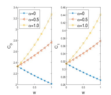
(a)

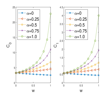
(b)

Figure 1: The values of $C_{0}$ and $C_{1}$ for different $w$. The plots on the left and right panels are respectively for $\rho$=0.5 and $\rho$=1. For $\alpha=0$, the coefficients decrease with $w$ and for any $\alpha\neq 0$ increase with $w$. The smallest values of $C_{0}$ and $C_{1}$ are obtained around $\alpha=0,w=1$. Note that coefficients are smaller for smaller $\rho$.

Since $C_{0}\epsilon$ term is controlled by $\epsilon$, for the reconstruction error to be small in (19), the multiplier $e$ of $C_{1}$ should be small, where $e=w\|x-x_{k}\|_{1}+(1-w)\|x_{T^{c}\cap T_{0}^{c}}\|_{1}+\|x_{T^{c}\cap T_{0}}\|_{1}$. The first two terms are small in the error expression as $x_{k}$ is the best-$k$-term approximation of $x$ and $T_{0}$ is the support of $x_{k}$ which can be further reduced by choosing optimal $w$. In order to make $e$ small, we need $\|x_{T^{c}\cap T_{0}}\|_{1}$ to be small. This is possible if $x_{T}$ contains the largest components of $x_{k}$ or the cardinality of $T^{c}\cap T_{0}$ is as small as possible. The latter case can happen when $\alpha\rho$ is close to 1. In application like in interior tomography, this condition translates to interior portion possessing dominating pixels. As the objective of the paper not is related to tomography, we do not go into the details of it any further.

We have computed the values of $e$ and $C_{1}e$ against different $\alpha$ and $w$, which are depicted in Fig. 2. Here $x$ has been taken to be a normalized vector from Gaussian distribution with previously stated values for $k$ and $\mu$. The plots in this figure indicate that $e$ is large for $\alpha=0$, and for a given $\alpha$, it increases with $w$. The smallest value for $e$ is obtained at $\alpha=1$. Again $C_{1}e$ is large for $\alpha=0$. For smaller values of $\alpha$, $C_{1}e$ decreases with $w$ and for $\alpha=0$, $C_{1}e$ decreases with $w$. This is due to the effect of $C_{1}$. Overall, the error-bound takes its minimum value around $\alpha=1$ and $w=0$.

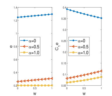
(a)

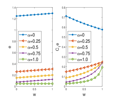
(b)

Figure 2: The values of $e$ and $C_{1}e$ for different $w$ and $\alpha$ values. These plots indicate that the dominant error term in (19) takes smaller values when $\alpha=1$ and $w=0$.

4.1 Comparison of bounds on $k$

Though the objective of present work is to propose an error bound restricted to a nonempty subset $T\subset[n]$, a natural question arises whether our $k$ bound in (18) is better behaved than the ones associated with the global error bounds in the standard case (4) and in the weighted case (10). We compare the $k$-bounds numerically in terms of a $k$-ratio. By a $k$-ratio in the standard case we mean the right hand side of our $k$-bound in (18) divided by its counterpart in (4). Similarly we consider the k-ratio in the weighted one norm case with respect to (10). Fig. 3 provides a comparison of $k$-ratios, which has been generated by considering, as examples, $\mu=0.1$, $\rho=0.5$ and $\rho=0.75$. It can be seen in both the cases that the $k$-ratios are strictly greater than 1 for all $w\in[0,1]$ and for all $\alpha\in[0,1]$. It is clear from the graphs that, even for larger values of $\rho$, our $k$ bound becomes less pessimistic than that of (4) and (10) for smaller values of $w$ for all $\alpha$. But since we are interested in finding error bounds on a subset $T$, which has a smaller size than the support of the best $k$-term approximation $T_{0}$, we do not consider the cases for larger values for $\rho$.

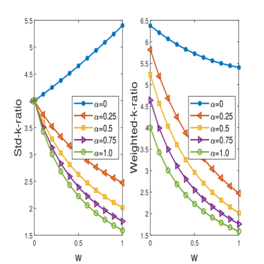
(a)

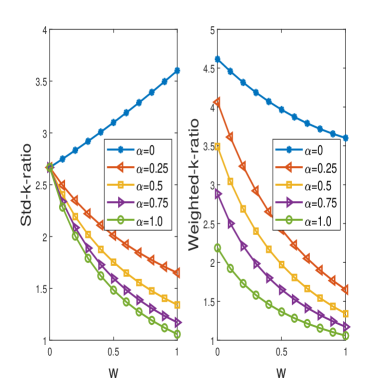
(b)

Figure 3: Comparison of $k$-ratios for $\rho=0.5$ and $\rho=0.75$ respectively. Note that in all cases $k$-ratio is strictly greater than 1, which indicates that our sufficient condition on sparsity $(k)$ is much weaker than that of the standard and weighted one norm cases.

4.2 Comparison of bounds on error

The local error bound in Theorem 3.1 (that is, (19)) becomes relevant if its right hand side is less than that of the global bounds in Theorems 2.2, 2.3, 2.4 and 2.5. Since the stated right hand sides are functions of the solution vector $x$ with various associated parameters and different underlying conditions, comparing them for a general solution vector $x\in\mathbf{R}^{n}$ does not look practical. In view of this, we try to compare the coefficients (i.e, $C_{0}$ and $C_{1}$ with their respective counterparts in Theorems 2.2, 2.3, 2.4 and 2.5) when the associated error expressions coincide. It is clear that the associated error parts coincide if $\|x_{T^{c}\cap T_{0}}\|_{1}$ is small. That is, $T$ contains largest magnitude entries from $T_{0}$. Consider a particular case for this in which $T=T_{0}$. In such a case, both the error terms associated with coefficients in global as well as local error bounds coincide. Hence in this case it is enough to compare the corresponding coefficients $C_{0}$ and $C_{1}$ (that is, $C_{0}$ and $C_{1}$ are respectively compared to $C_{0}^{(i)}$ and $C_{0}^{(i)}$ for $i=1,2,3,4$).

The coefficients in (12) and (20) can be compared directly as both of them are in terms of mutual coherence parameter $\mu$. The coefficients in (9), (14) and (17) are in terms of the RIC and ROC. In order to compare them with the corresponding ones in (20) which are in terms of $\mu$, we use the upper bounds [2][5]: $\theta_{k,k}\leq\delta_{2k}$ and $\delta_{k}\leq(k-1)\mu$. For comparing with (9) we need a constant $a$ such that $a>1$ and $ak\in\mathbb{Z}$. We take a simple choice $a=2$. Again, for comparison with (14), we need two constants $a$ and $b$. We set these to $k$, which is permissible. Finally, for comparing with (17), we need a constant $t>d$. In our case, as $d=1$, we take a simple choice $t=2$. The plots in Fig. 4, comparing the coefficients in the stated setting, are denoted through the legends ‘Local’, ‘Global(1), Global(2), Global(3) and Global(4), which stand respectively for the coefficients in (20), (12),(9),(14) and (17). From Fig 4, it is clear that our coefficients being much small imply that the right hand side of our bound is small compared to their global bounds at least in the case where $T$ contains the indices corresponding to largest magnitude entries in $x$ for all $w\in[0,1]$. As highlighted already, comparison of bounds in other cases does not look possible.

In generating Fig 4, we have taken $\mu=0.1$ and $k=2$. It may be noted that the coefficients in (9) are negative for $w>0.8$ and in (14), $w=0$ gives $s=0$ which makes $C_{0}^{(3)}$ in (14) not defined at $w=0$.

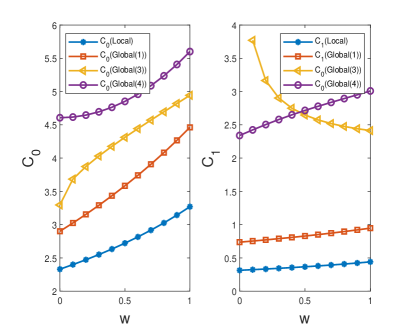
(a)

(b)

Figure 4: Comparison of the coefficients when the terms associated with them coincide. Note that both coefficients corresponding to our local bound are less than the corresponding ones in other bounds, when the partial support $T$ contains the indices corresponding to largest magnitude entries of the solution $x$.

5 Conclusion

The present work has proposed a local recovery bound for prior support constrained compressed sensing, while the existing bounds are global in nature. In particular, an error estimate restricted to prior support, providing recovery guarantee, has been provided along with a bound on the sparsity of the solution to be recovered.

Acknowledgments:
The first author is thankful to the UGC, Government of India, (JRF/2016/409284) for its financial support. The second author gratefully acknowledges the support received from the MHRD, Government of India.

References

- [1] Tony Tony Cai, Lie Wang, and Guangwu Xu. Stable recovery of sparse signals and an oracle inequality. IEEE Transactions on Information Theory, 56(7):3516–3522, 2010.
- [2] E. J. Candes and T. Tao. Decoding by linear programming. IEEE Transactions on Information Theory, 51(12):4203–4215, 2005.
- [3] Wengu Chen and Yaling Li. Recovery of signals under the condition on ric and roc via prior support information. ArXiv, abs/1603.03465, 2016.
- [4] David L Donoho and Xiaoming Huo. Uncertainty principles and ideal atomic decomposition. IEEE transactions on information theory, 47(7):2845–2862, 2001.
- [5] Michael Elad. Sparse and redundant representations: from theory to applications in signal and image processing. Springer Science & Business Media, 2010.
- [6] C.A. Berenstein F. R. Rashid Farrokhi, K. J. R. Liu and D. Walnut. Wavelet based multi resolution local tomography. IEEE Trans. Image Process, 6(7):1412–1430, 1997.
- [7] M. P. Friedlander, H. Mansour, R. Saab, and Ö. Yilmaz. Recovering compressively sampled signals using partial support information. IEEE Transactions on Information Theory, 58(2):1122–1134, 2012.
- [8] Huanmin Ge and Wengu Chen. Recovery of signals by a weighted ℓ2/ℓ1 minimization under arbitrary prior support information. Signal Process., 148:288–302, 2018.
- [9] Boris Kashin and V. Temlyakov. A remark on compressed sensing. Mathematical Notes, 82:748–755, 11 2007.
- [10] Esther Klann, Eric Quinto, and Ronny Ramlau. Wavelet methods for a weighted sparsity penalty for region of interest tomography. Inverse Problems, 31:025001, 02 2015.
- [11] Haixiao Liu, Bin Song, Fang Tian, and Hao Qin. Compressed sensing with partial support information: coherence-based performance guarantees and alternative direction method of multiplier reconstruction algorithm. IET Signal Processing, 8(7):749–758, 2014.
- [12] P. V. Jampana R. R. Naidu and C S Sastry. Deterministic compressed sensing matrices: Construction via euler squares and applications. IEEE Trans. on Signal Processing, 64:3566–3575, 2016.
- [13] C S Sastry and P. C. Das. A convolution backprojection algorithm for local tomography. ANZIAM, 46(7):341–360, 2005.
- [14] Namrata Vaswani and Wei Lu. Modified-cs: Modifying compressive sensing for problems with partially known support. IEEE Transactions on Signal Processing, 58(9):4595–4607, 2010.