Instanton - motivated study of spontaneous fission of odd-A nuclei

Abstract

Using the idea of the instanton approach to quantum tunneling we try to obtain a method of calculating spontaneous fission rates for nuclei with the odd number of neutrons or protons. This problem has its origin in the failure of the adiabatic cranking approximation which serves as the basis in calculations of fission probabilities. Selfconsistent instanton equations, with and without pairing, are reviewed and then simplified to non-selfconsistent versions with phenomenological single-particle potential and seniority pairing interaction. Solutions of instanton-like equations without pairing and actions they produce are studied for the Woods-Saxon potential along realistic fission trajectories. Actions for unpaired particles are combined with cranking actions for even-even cores and fission hindrance for odd-$A$ nuclei is studied in such a hybrid model. With the assumed equal mass parameters for neighbouring odd-A and even-even nuclei, the model shows that freezing the $K^{\pi}$ configuration leads to a large overestimate of the fission hindrance factors. Actions with adiabatic configurations mostly show not enough hindrance; instanton-like actions for blocked nucleons correct this, but not sufficiently.

I Introduction

Nuclear fission is thought to be a collective process, classically envisioned in analogy to fragmentation of a liquid drop. In reactions induced by neutrons and light or heavy ions, fission is one of many possible deexcitation channels of a formed compound nucleus. On the other hand, spontaneous fission is a decay of the nuclear ground state (g.s.) which exhibits its meta-stability and involves quantum tunneling through a potential barrier. In a theoretical approach, the fission barrier follows from a model of the shape-dependent nuclear energy. In practical terms, it is calculated either from a selfconsistent mean-field functional or a microscopic-macroscopic model, as a landscape formed by the lowest energies $E({\bf q})$ at fixed values of a few arbitrarily chosen coordinates ${\bf q}=(q_{1},...,q_{i},...)$ (for simplicity assumend dimensionless) describing nuclear shape. The obscure part of the current approach relates to a) the likely insufficiency of included coordinates and b) a description of tunneling dynamics, essentially shaped after the Gamow method, but without a clear understanding of mass parameters and conjugate momenta entering the formula for decay rate.

The experimentally well established presence of pairing correlations in nuclei gives rationale for using cranking Inglis ; Funny or adiabatic Time-Dependent Hartree-Fock(-Bogolyubov) - ATDHF(B) - approximation BV ; GQ ; DS in the description of fission in even-even (e-e) nuclei. Indeed, as the lowest two-quasiparticle excitation in such nuclei has energy of at least twice the pairing gap $2\Delta$, which in heavy nuclei amounts to more than 1 MeV, one can, for collective velocities $|\hbar{\dot{\bf q}}|$ reasonably smaller than that, solve the time-dependent Schrödinger (or mean-field) equation to the first order in ${\dot{\bf q}}$ and obtain kinetic energy of shape changes: $\frac{1}{2}\sum_{ij}B_{q_{i}q_{j}}({\bf q}){\dot{q}}_{i}{\dot{q}}_{j}$, with cranking (or ATDHFB) mass parameters $B_{q_{i}q_{j}}({\bf q})$. Then one can apply the Jacobi variational principle to the imaginary under-the-barrier motion in order to find the quasiclassical tunneling path ${\bf q}(\tau)$ by minimizing action:

$$S\left[{\bf q}(\tau)\right]=\int_{{\bf q}_{ini}}^{{\bf q}_{fin}}\sum_{i}p_{i}dq_{i}=\int_{q_{ini}}^{q_{fin}}\sqrt{2B_{qq}({\bf q}(\tau))[E({\bf q}(\tau))-E_{0}]}\,dq.$$ (1)

Here, $p_{i}=\sum_{j}B_{q_{i}q_{j}}({\bf q})\dot{q}_{j}$ are the conjugate momenta; $q$ (without index) is an effective coordinate along a path, usually the one of $q_{i}$ that controls elongation of the nucleus; $B_{qq}=\sum_{kl}B_{q_{k}q_{l}}\frac{dq_{k}}{dq}\frac{dq_{l}}{dq}$ is the effective mass parametr along the fission path with respect to $q$. The Jacobi principle requires that a) ${\bf q}_{ini}$ and ${\bf q}_{fin}$ - the initial and final points of the path through a barrier - be fixed for all tunneling paths and b) on each trial path, $E({\bf q})-\frac{1}{2}\sum_{ij}B_{q_{i}q_{j}}({\bf q}){\dot{q}}_{i}{\dot{q}}_{j}$ (the potential minus kinetic energy) be constant and equal to $E_{0}=E({\bf q}_{ini})=E({\bf q}_{fin})$, usually chosen as $E_{g.s.}+E_{zp}$ - the g.s. energy augmented by the zero-point energy of oscillations around the g.s. minimum in direction of fission, $E_{zp}=\frac{1}{2}\hbar\omega_{0}$. The spontaneous fission rate is given to the leading order by: $(\frac{\omega_{0}}{2\pi})e^{-2S_{min}/\hbar}$, with $S_{min}$ - the minimal action. By the first equality in (1), $S$ equals the integral of twice the collective kinetic energy, $B_{qq}{\dot{q}}^{2}$, with $(\hbar{\dot{q}})^{2}=\frac{2[E(q)-E_{0}]}{B_{qq}}$, over the time of passing the barrier. Estimating a posteriori collective velocities of the fictitious under-barrier motion for heavy nuclei, with typical cranking mass parameter for the Woods-Saxon potential, $B_{qq}\gtrsim 200\hbar^{2}$/MeV, and the fission barrier $\lesssim 7$ MeV, one obtains $\hbar{\dot{q}}\lesssim 0.25$ MeV, so the error of the cranking approximation might be believed moderate.

Situation changes rather dramatically for odd-$Z$ or/and odd-$N$ nuclei. For odd number of particles, their contribution to the cranking mass parameter $B_{q_{i}q_{j}}$, derived as if the adiabatic approximation were legitimate, reads:

$$B_{q_{i}q_{j}} = 2\hbar^{2}\Bigg{[}\sum_{\mu,\nu\neq\nu_{0}}\frac{\langle\mu\mid\frac{\partial{\hat{h}}}{\partial q_{i}}\mid\nu\rangle\langle\nu\mid\frac{\partial{\hat{h}}}{\partial q_{j}}\mid\mu\rangle}{\left(E_{\mu}+E_{\nu}\right)^{3}}\left(u_{\mu}v_{\nu}+u_{\nu}v_{\mu}\right)^{2}$$

$$+ \frac{1}{8}\sum_{\nu\neq\nu_{0}}\frac{\left(\tilde{\epsilon}_{\nu}\frac{\partial\Delta}{\partial q_{i}}-\Delta\frac{\partial\tilde{\epsilon}_{\nu}}{\partial q_{i}}\right)\left(\tilde{\epsilon}_{\nu}\frac{\partial\Delta}{\partial q_{j}}-\Delta\frac{\partial\tilde{\epsilon}_{\nu}}{\partial q_{j}}\right)}{E_{\nu}^{5}}\Bigg{]}$$

$$+ 2\hbar^{2}\sum_{\nu\neq\nu_{0}}\frac{\langle\nu\mid\frac{\partial{\hat{h}}}{\partial q_{i}}\mid\nu_{0}\rangle\langle\nu_{0}\mid\frac{\partial{\hat{h}}}{\partial q_{j}}\mid\nu\rangle}{\left(E_{\nu}-E_{\nu_{0}}\right)^{3}}\left(u_{\nu}u_{\nu_{0}}-v_{\nu}v_{\nu_{0}}\right)^{2}.$$

Here, the odd nucleon occupies the orbital $\nu_{0}$ in the g.s.; ${\hat{h}}$ is the mean-field single - particle (s.p.) Hamiltonian, $\epsilon_{\mu}$ are its eigenenergies, $\tilde{\epsilon}_{\nu}=\epsilon_{\nu}-\lambda$, $E_{\mu}=\sqrt{\tilde{\epsilon}_{\mu}^{2}+\Delta^{2}}$, $u$ and $v$ are the usual BCS amplitudes. A common pairing gap $\Delta$ and Fermi energy $\lambda$ were assumed for the g.s. and its two-quasiparticle excitations: those with the odd particle in the state $\nu_{0}$ which give contribution in the square bracket that has the same form as the mass parameter for an e-e nucleus, and those with the odd particle in the state $\nu\neq\nu_{0}$ and the orbital $\nu_{0}$ paired, given by the last term of the formula. The latter becomes nearly singular, $\sim(E_{\nu_{0}}-E_{\nu})^{-3}$, at close avoided level crossings where $E_{\nu_{0}}-E_{\nu}$ can be of the order of keV or less. This invalidates the very assumption underlying the cranking formula, except for ridiculously small collective velocities. But there is still another deficiency: a departure from the symmetry preserved on a part of the fission trajectory often produces a negative contribution to the inertia parameter whose magnitude would depend on the proximity of the relevant crossing of levels of different symmetry classes. Although some calculations of fission half-lives for odd nuclei with the cranking mass parameters (I) were done in the past, e.g. Lojew , the above-mentioned problems make the precise minimization of action (1) for those nuclei both questionable and practically very difficult - a good illustration of near-singular cranking mass parameter [calculated with a formula more refined than (I)] in the odd nucleus is provided in Mirea2019 (the middle panel of Fig. 4 there) foot1 .

The well known experimental evidence, reviewed recently in Hess , shows that the spontaneous fission rates of odd nuclei are three to five orders of magnitude smaller than those of their e-e neighbours. Although the explanation usually invokes the specialization energy - an increase in the fission barrier by the blocking of one level by a single nucleon - a quantitative understanding is lacking at present. In particular, the combination of axial symmetry of the nuclear deformation and very different densities of s.p. levels with low- and high-$\Omega$ quantum numbers ($\Omega$ being the projection of the s.p. angular momentum on the symmetry axis of a nucleus) could suggest a higher specialization energy, and thus smaller fission rate, for configurations based on high-$\Omega$ orbitals, but the data Hess contradict this.

While estimates of fission half-lives rely on the assumption of nearly adiabatic motion, doubtful for odd-$A$ nuclei, the real-time solutions of Schrödinger-like dynamics are regular for any velocity profile ${\dot{\bf q}}$ and any avoided crossings. In general, they lead to a population of levels above the Fermi energy. Analogous possibility must exist in the fictitious imaginary-time motion, pertinent to quantum tunneling. In this light, a consideration of non-adiabatic tunneling - with fission paths formed at least in part by non-adiabatic configurations - presents itself as an interesting subject. Beyond-cranking effects could provide corrections to the standard cranking spontaneous fission rates in e-e nuclei and can be crucial for spontaneous fission of odd-$A$ nuclei and high-$K$ isomers

In this paper, we present an attempt towards replacing the adiabatic cranking approximation by a scheme including non-adiabatic fission paths, motivated by the instanton method Coleman ; LNP ; Neg1 ; PudNeg ; Neg2 . Instantons are solutions with the infinite period to time-dependent mean-field equations in imaginary time $\tau=it$, with the nuclear g.s. wave function as the boundary value. They arise from the saddle-point approximation to the path integral representation of the propagator and give the leading contribution to spontaneous fission rate of the form: $A_{inst}\exp(-S_{inst}/\hbar)$. Here, $S_{inst}$ - instanton action, is the counterpart of $2S\left[{\bf q}(\tau)\right]$ in (1), while the prefactor $A_{inst}$ - the ratio of determinants including frequencies of quadratic fluctuations around the instanton and the g.s. - for review see e.g. ChT ; Ander ; tunnsplit - will not be considered it in the following. The instanton with the smallest action (there can be more than one as the instanton equation determines local minima of action) gives fission half-life without the necessity of defining mass parameters. The resulting fission path involves all degrees of freedom of the mean-field state, not only shape parameters.

The difficulty in solving for a selfconsistent instanton including pairing is beyond that of solving real-time TDHFB equations: the generically exponential $\tau$-dependence of the HFB $Z$ matrix Ring , introducing components differing by orders of magnitude, has to be found from equations non-local in $\tau$ (see Sect. II.3). Here, we treat the selfconsistent theory as a motivation, and solve imaginary-time-dependent Schrödinger equation (iTDSE) with the phenomenological Woods-Saxon (W-S) potential to calculate action along various chosen paths. We use micro-macro energy for $E({\bf q})$. Since we reject cranking mass parameters for odd-$A$ nuclei, we have to provide ${\dot{\bf q}}$ without them. To this aim we use cranking mass parameters of the neighbouring e-e nucleus. With this prescription, we can calculate manifestly beyond-cranking actions and study their behaviour. Although we formulate equations with pairing, in the present paper we present iTDSE instanton-like solutions without it. To the best of our knowledge, such solutions and their actions are discussed for the first time. Then, we combine instanton-like solutions for the odd nucleon with the cranking action with pairing for the e-e core in a hybrid model to study fission hindrance in odd-$A$ nuclei. Within this model we calculate and compare fission half-lives obtained with and without constraining the $\Omega^{\pi}$ (with $\pi$ - parity) g.s. configuration.

The presented approach cannot be as yet a basis for the systematic minimization of action over fission paths. Moreover, it differs from the instanton method by ignoring the anti-hermitean part of the imaginary-time mean-field. We think, however, that it presents some features of the instanton method and may be useful for developing either a more refined non-selfconsistent method or ways to implement the selfconsistent instanton treatment of spontaneous fission half-lives, including odd-$A$ nuclei and high-$K$ isomers.

The paper is organized as follows: in sect. II we briefly describe the instanton formalism with and without pairing, specifying a simplification of each of them to a non-selfconsistent version with the phenomenological s.p. potential. To provide an illustration of imaginary-time solutions, in sect. III we discuss the two-level model, in particular the dependence of action on the interaction between levels and the collective velocity. Properties of solutions and actions obtained from the iTDSE with the realistic W-S potential are described in sect. IV, including an example of the action calculation along the path through non-axial deformations. Sect. V contains a study of the fission hindrance in odd nuclei made within a hybrid model utilizing adiabatic cranking action for the e-e core and the iTDSE action without pairing for the odd nucleon. This approach is meant to mimic a model with pairing which we have not solved yet. As a byproduct, we study the effect of freezing the configuration along the path of axially-symmetric deformations on the fission rate. This is done under the assumption that the collective velocity along a given path in odd-$A$ nucleus is as if it had the mass parameter of the e-e neighbour; stated otherwise, the difference in ${\dot{q}}$ between the odd-$A$ nucleus and its e-e $A-1$ neighbour comes solely from their different fission barriers. Summary and conclusions are given in sect. VI. In appendices we derive expressions for the Floquet exponent and action for periodic solutions within the cranking approximation (Appendix A), describe the method of solution of the iTDSE (Appendix B), tests of the reliability of the calculated actions (Appendix C) and the problem of calculating action along paths through non-axial shapes (Appendix D).

II Instanton-motivated approach

The instanton approach to nuclear fission was formulated in the mean-field setting in LNP ; Neg1 ; JS1 ; JS ; JS2 . After reviewing the selfconsistent formulation without pairing in Subsect. A, in Subsect. B, we formulate the non-selfconsistent version with the phenomenological nuclear potential, the solutions to which we present in this work. For completeness, as the pairing interaction is crucial to nuclear fission, we review also the selfconsistent equations with pairing in Subsect. C, and formulate the model with the phenomenological potential and the monopole pairing with the selfconsistent pairing gap in Subsect. D.

II.1 Instantons of Hartree-Fock equations

A transition to imaginary time, $t\rightarrow-i\tau$, transforms TDHF equations for s.p. amplitudes $\psi_{k}(t)$ into imaginary-TDHF (iTDHF) equations for amplitudes $\phi_{k}(x,\tau)=\psi_{k}(x,-i\tau)$, with the complex-conjugate amplitudes $\psi^{*}_{k}(t)$ becoming $\psi^{*}_{k}(x,-i\tau)=\phi^{*}_{k}(x,-\tau)$, so that the scalar products $\langle\psi_{k}(t)|\psi_{l}(t)\rangle$ transform to $\langle\phi_{k}(-\tau)|\phi_{l}(\tau)\rangle$. Mean-field solutions dominating the quasiclassical tunneling rate are periodic LNP ; Neg1 , hence the iTDHF equations acquire the additional terms $\zeta_{k}\phi_{k}$, with $\zeta_{k}$ - Floquet exponents with the dimension of energy, which ensure periodicity:

$$\hbar\frac{\partial\phi_{k}({\tau})}{\partial\tau}=-(\hat{h}(\tau)-\zeta_{k})\phi_{k}(\tau).$$ (3)

The mean-field hamiltonian $\hat{h}(\tau)=\hat{h}[\phi^{*}(-\tau),\phi(\tau)]$ is defined by: $\hat{h}(\tau)\phi_{k}(\tau)=\delta\mathcal{H}/\delta\phi^{*}_{k}(-\tau)$, where $\mathcal{H}(\tau)$ is the energy overlap $\langle\Phi(-\tau)|\hat{H}|\Phi(\tau)\rangle$, playing the same role as energy in the usual TDHF,

$$\mathcal{H}(\tau)=\mathcal{H}[\phi^{*}(-\tau),\phi(\tau)]=\int d^{3}x\left\{\sum_{k\ occ}\frac{\hbar^{2}}{2m}\nabla\phi_{k}^{*}(-\tau)\nabla\phi_{k}(\tau)+\mathcal{V}[\phi^{*}(-\tau),\phi(\tau)]\right\},$$ (4)

with $\mid\Phi(\tau)\rangle$ - the Slater determinant built of occupied orbitals $\{\phi_{k}(\tau)\}$, and $\mathcal{V}$ - a two-body interaction energy density composed as in the HF, but with $\phi_{k}(\tau)$ in place of $\psi_{k}(t)$, and $\phi^{*}_{k}(-\tau)$ in place of $\psi^{*}_{k}(t)$. The instanton solving (3) that describes quantum tunneling, called bounce, has to fulfil specific consditions: amplitudes at the boundary are equal to static Hartree-Fock (HF) solutions at the metastable state (m.s.) minimum, $\phi_{k}(-T/2)=\phi_{k}(T/2)=\psi_{k}^{HF}$, with HF energy $E_{m.s.}$, while the states $\phi_{k}(\tau=0)$ form a normalized Hartree-Fock state with the same energy $E_{m.s.}$ at the outer slope of the barrier, that corresponds to the exit point from the barrier ${\bf q}_{fin}$ in Eq. (1). An infinite period $T$ corresponds to a decay from the m.s. - evolution becomes infinitely slow close to the m.s. minimum. Hence, $\partial\phi_{k}/\partial\tau$ become zero as $\tau\rightarrow\pm\infty$, and Eq. (3) reduce there to the static HF equations. So, in the selfconsitent theory, the Floquet exponents are equal to s.p. energies at the m.s. state.

Both, energy overlaps $\mathcal{H}(\tau)$ and the mean-field Hamiltonian $\hat{h}(\tau)$, depend on $\phi_{k}(\tau)$ and $\phi_{k}(-\tau)$, so Eq. (3) are nonlocal in $\tau$ and one cannot solve them as an initial value problem. Together with the periodicity condition, this makes iTDHF equations a kind of a nonlinear boundary value problem in four dimensions.

Eq. (3) conserve energy overlap $\mathcal{H}(\tau)$, diagonal overlaps of solutions, and give the exponential $\tau$-dependence to their non-diagonal overlaps. As the HF solutions at the boundary are orthonormal, so remain the bounce solutions:

$$\langle\phi_{i}(-\tau)|\phi_{j}(\tau)\rangle=\delta_{ij}.$$ (5)

From $\hat{H}^{\dagger}=\hat{H}$, one has $\mathcal{H}(-\tau)=\mathcal{H}^{*}(\tau)$, and the mean field hamiltonian $\hat{h}(\tau)$ is in general not hermitean, but fulfils the condition: $\hat{h}(-\tau)=\hat{h}^{\dagger}(\tau)$. It may be presented as a sum of its hermitean and antihermitean parts, $\hat{h}(\tau)=\hat{h}_{R}(\tau)+\hat{h}_{A}(\tau)$, with: $\hat{h}_{R}(-\tau)=\hat{h}_{R}(\tau)=\hat{h}_{R}^{\dagger}(\tau)$ and $\hat{h}_{A}(-\tau)=-\hat{h}_{A}(\tau)=\hat{h}_{A}^{\dagger}(\tau)$; the $\tau$-odd, antihermitian part $\hat{h}_{A}$ comes from $\tau$-odd parts of densities building energy overlap $\mathcal{H}(\tau)$. In tunneling, at least one $\tau$-odd density is provided by the current density $\mathbf{j}$, in imaginary time given by: $\mathbf{j}(\tau)=\sum_{k}[\phi_{k}(\tau)\nabla\phi_{k}^{*}(-\tau)-\phi_{k}^{*}(-\tau)\nabla\phi_{k}(\tau)]/2$, JS , fulfiling: $\mathbf{j}(-\tau)=-\mathbf{j}^{*}(\tau)$. Decomposing amplitudes into $\tau$-even and $\tau$-odd parts, $\phi_{k}(\tau)=\varphi_{k}(\tau)-\xi_{k}(\tau)$, $\phi_{k}(-\tau)=\varphi_{k}(\tau)+\xi_{k}(\tau)$, one has:

$${\bf j}=\sum_{k\ occ}\left[\Re(\varphi^{*}_{k}\nabla\xi_{k}-\xi^{*}_{k}\nabla\varphi_{k})+i\Im(\xi^{*}_{k}\nabla\xi_{k}-\varphi^{*}_{k}\nabla\varphi_{k})\right].$$ (6)

One can see that, even if $\phi_{k}$ are purely real, the $\tau$-odd components $\xi_{k}$ in the first part of this expression generate the $\tau$-odd antihermitean mean field ${\hat{h}}_{A}$. For small collective velocities, the $\tau$-odd mean field ${\hat{h}}_{A}$ is a direct analogy in the imaginary-time formalism of the Thouless-Valatin potential of the ATDHF method in real time ThouVal .

After finding iTDHF solutions one can calculate action. Since in the mean-field theory with a Slater determinant $\Psi(t)$, $\langle\Psi(t)\mid i\hbar\partial_{t}-{\hat{H}}\mid\Psi(t)\rangle$ plays a role of Lagrangian, action $\int dt\langle\Psi(t)\mid i\hbar\partial_{t}\mid\Psi(t)\rangle$ in the imaginary-time version becomes LNP ; Neg1 :

$$S=\hbar\int_{-T/2}^{T/2}d\tau\sum\limits_{i=1}^{N}\left\langle\phi_{i}(-\tau)\big{|}\partial_{\tau}\phi_{i}(\tau)\right\rangle=\int_{-T/2}^{T/2}d\tau\sum\limits_{i=1}^{N}\left\langle\phi_{i}(-\tau)\big{|}\zeta_{i}-\hat{h}(\tau)\big{|}\phi_{i}(\tau)\right\rangle,$$ (7)

where the summation runs over the occupied s.p. states.

Contrary to the unfortunate and erroneous statement in JS [in the paragraph containing the formula (14) there], repeated in JS2 [after the formula (7) there], this expression is obviously composed of changes in $\phi_{i}(\tau)$ parallel to $\phi_{i}(-\tau)$.

II.2 Non-selfconsistent instanton-motivated approach

In order to gain some idea about solutions of imaginary-time-dependent Schrödinger-like equations with instanton boundary conditions and resulting actions we replace the mean-field hamiltonian ${\hat{h}}[\phi^{*}(-\tau),\phi(\tau)]$ by a simple one with the phenomenological W-S s.p. potential. Releasing the selfconsistency makes these equations linear iTDSEs and removes non-locality in $\tau$, thus considerably simplifying solution. Certainly, we lose generality: the non-hermitean nature of the mean potential in tunneling is lost, we have to resort to the usual paramerization of nuclear shapes and have to externally provide the collective velocity ${\dot{q}}(\tau)$ which in the selfconsistent theory would follow from the energy constraint $\mathcal{H}(\tau)=E_{m.s.}$. However, we gain a possibility to study iTDSE solutions and their actions for manifestly non-adiabatic imaginary-time motions along trial fission paths which in current treatments of fission are commonly considered realistic. To have an approximate energy conservation we assume the effective collective velocity given by:

$$B^{even}_{qq}(q){\dot{q}}^{2}=2(E(q)-E_{m.s.}),$$ (8)

with:

$$d\tau=\frac{dq}{{\dot{q}}(\tau)}.$$ (9)

Here, $E(q)$ is the microscopic-macroscopic energy and $B^{even}_{qq}(q)$ is the adiabatic mass parameter along the fission path of the even - even nucleus - the one in question or the nearest neighbour in case of the odd-$A$. The motivation will be given in section V.2. This whole procedure may be viewed as an attempt to simplify the selfconsistent theory to a micro-macro version.

As a result, the phenomenological s.p. Hamiltonian ${\hat{h}}(\tau)$ is:

$${\hat{h}}(q(\tau))=-\frac{\hbar^{2}}{2m}\nabla^{2}+V(q(\tau)),$$ (10)

where $V$ is the phenomenological s.p. potential, including Coulomb repulsion for protons, depending on the collective coordinate $q$ which itself depends on $\tau$. In solving the equation (3) with the above s.p. hamiltonian along a given path we restrict to the subspace spanned by ${\cal N}$ adiabatic s.p. orbitals $\psi_{\mu}(q)$. In this subspace, there are ${\cal N}$ bounce solutions $\phi_{i}(\tau)$, each of which tends to the s.p. orbital $\psi_{i}(q_{min})$ at the metastable minimum as $T\rightarrow\pm\infty$. By expanding these solutions onto adiabatic orbitals

$$\phi_{i}(\tau)=\sum_{\mu}C_{\mu i}(\tau)\psi_{\mu}(q(\tau)),$$ (11)

we obtain the following set of equations for the square matrix of the coefficients $C_{\mu i}(\tau)$:

$$\hbar\frac{\partial C_{\mu i}}{\partial\tau}+{\dot{q}}\sum_{\nu}\langle\psi_{\mu}(q(\tau))\mid\frac{\partial\psi_{\nu}}{\partial q}(q(\tau))\rangle C_{\nu i}=[\zeta_{i}-\epsilon_{\mu}(q(\tau))]C_{\mu i}.$$ (12)

Here, $\zeta_{i}$, $i=1,...,{\cal N}$, are the Floquet exponents in imaginary time, which for the selfconsistent instanton would be eqal to the s.p. energies at the metastable minimum, $\zeta_{i}=\epsilon_{i}(q_{min})$. However, for a finite imaginary-time interval $[-T/2,T/2]$, $\zeta_{i}\neq\epsilon_{i}(q_{min})$, although they should tend to this limit when $T\rightarrow\infty$.

The conservation of overlaps $\langle\phi_{i}(-\tau)\mid\phi_{j}(\tau)\rangle=\delta_{ij}$ leads to the condition on $C_{\mu l}(\tau)$:

$$\sum_{\mu=1}^{{\cal N}}C^{*}_{\mu i}(-\tau)C_{\mu j}(\tau)=\delta_{ij}.$$ (13)

This means that the matrix $C_{\mu i}(\tau)$ has the inverse $C^{+}(-\tau)$ and the adiabatic states can be expanded on (all ${\cal N}$) bounce states:

$$\psi_{\mu}(q(\tau))=\sum_{i=1}^{{\cal N}}C^{*}_{\mu i}(-\tau)\phi_{i}(\tau)=\sum_{i=1}^{{\cal N}}C^{*}_{\mu i}(\tau)\phi_{i}(-\tau),$$ (14)

where in the second equality we assumed that $q(\tau)=q(-\tau)$ which strictly holds for any real bounce observable: $q(\tau)=\sum_{i\ occ}\langle\phi_{i}(-\tau)\mid{\hat{q}}\mid\phi_{i}(\tau)\rangle=q^{*}(-\tau)$. Then, the orthonormality of $\psi_{\mu}$, combined with the overlaps Eq. (13), produces the relation:

$$\sum_{i=1}^{\cal N}C_{\mu i}(\tau)C^{*}_{\nu i}(-\tau)=\delta_{\mu\nu}.$$ (15)

Thus, the quantity $p_{\mu i}(\tau)=C^{*}_{\mu i}(-\tau)C_{\mu i}(\tau)$ may be considered as a quasi-occupation (it can be negative or complex in general case) of the adiabatic level $\mu$ in the bounce solution $i$, with $\sum_{\mu}p_{\mu i}(\tau)=1$, or as the quasi-occupation of the bounce state $i$ in the adiabatic state $\mu$, where $\sum_{i}p_{\mu i}(\tau)=1$. The sums over the occupied states: $\sum_{i\ occ}p_{\mu i}(\tau)$ are diagonal elements $\rho_{\mu\mu}(\tau)$ of the density matrix $\rho_{\mu\nu}(\tau)$ determined by the Slater states $\mid\Phi(\tau)\rangle$.

From (11) and (14) one obtains the relation:

$$\phi_{i}(-\tau)=\sum_{j=1}^{\cal N}\left(\sum_{\mu}^{\cal N}C_{\mu i}(-\tau)C^{*}_{\mu j}(-\tau)\right)\phi_{j}(\tau)=\sum_{j}^{\cal N}\left(C^{+}(-\tau)C(-\tau)\right)_{ji}\phi_{j}(\tau),$$ (16)

where the matrix $C^{+}(-\tau)C(-\tau)$ is hermitean and positive. One can define: $C^{+}(-\tau)C(-\tau)=\exp(2{\hat{\cal S}}(\tau))^{T}$, so that ${\hat{\cal S}}(\tau)$ is $\tau$-odd and hermitean and:

$$\phi_{i}(-\tau)=\exp({\hat{\cal S}}(\tau))\psi_{0i}(\tau),\hskip 8.53581pt\phi_{i}(\tau)=\exp(-{\hat{\cal S}}(\tau))\psi_{0i}(\tau),$$ (17)

where the states $\psi_{0i}(\tau)$ are $\tau$-even and orthonormal, so they could be considered as some ”mean” TDHF orbitals related to the bounce solutions $\phi_{i}(\tau)$ JS .

Action is equal to the sum over the occupied iTDHF solutions:

$$S=\Re\sum_{i\ occ}\int_{-T/2}^{T/2}\langle\phi_{i}(-\tau)\mid\zeta_{i}-{\hat{h}}\mid\phi_{i}(\tau)\rangle=\int_{-T/2}^{T/2}\sum_{i\ occ}\sum_{\mu=1}^{\cal N}[\zeta_{i}-\epsilon_{\mu}(q(\tau))]C^{*}_{\mu i}(-\tau)C_{\mu i}(\tau)d\tau,$$ (18)

so, using the quasi-occupations $p_{\mu i}$, it can be written as:

$$S=\int_{-T/2}^{T/2}\sum_{i\ occ}\sum_{\mu=1}^{\cal N}[\zeta_{i}-\epsilon_{\mu}(q(\tau))]p_{\mu i}(\tau)d\tau.$$ (19)

From this, the sum of actions for all individual s.p. bounce states is the integral of a difference between two sums: of all Floquet exponents and all adiabatic s.p. energies: $\sum_{i=1}^{\cal N}(\zeta_{i}-\epsilon_{i})$. It can be shown that this integral vanishes foot2 , so the sum of all actions is zero.

When the collective motion is nearly adiabatic, one recovers from this formalism action (1) with the cranking mass parameter and, ususally not mentioned, related formula for the Floquet exponent - see Appendix A.

II.3 Instantons with pairing interaction

In the presence of pairing interaction a proper mean-field formalism is the imaginary-time-dependent HFB (iTDHFB) method. The Bogolyubov transformation from the fixed, independent of time creation operators $a_{\mu}^{\dagger}$ to time-dependent quasiparticle creation operators $\alpha_{i}^{\dagger}(t)$, after passing to imaginary time $t\rightarrow-i\tau$, can be written JS :

$$\alpha_{i}^{\dagger}(\tau) = \sum_{\mu}(A_{\mu i}(\tau)a_{\mu}^{{\dagger}}+B_{\mu i}(\tau)a_{\mu}),$$

$$\alpha_{i}(-\tau) = \sum_{\mu}(A_{\mu i}^{*}(-\tau)a_{\mu}+B_{\mu i}^{*}(-\tau)a_{\mu}^{{\dagger}}),$$ (20)

where amplitudes $A_{\mu i}(t)$ i $B_{\mu i}(t)$ became functions of $\tau$, and their complex conjugate $A_{\mu i}^{*}(t)$ and $B_{\mu i}^{*}(t)$ depend now on $-\tau$. The unitarity of the Bogolyubov trnsformation in real time translates to the following condition in imaginary time:

$$\left(\begin{array}[]{cc}A^{T}(\tau),&B^{T}(\tau)\\ B^{\dagger}(-\tau),&A^{\dagger}(-\tau)\\ \end{array}\right)^{-1}=\left(\begin{array}[]{cc}A^{*}(-\tau),&B(\tau)\\ B^{*}(-\tau),&A(\tau)\\ \end{array}\right).$$ (21)

The hamiltonian overlap $\langle\Phi(\tau)\mid{\hat{H}}\mid\Phi(-\tau)\rangle$ can be expressed by the following contractions:

$$\langle\Phi(\tau)\mid a^{+}_{\nu}a_{\mu}\mid\Phi(-\tau)\rangle =\rho_{\mu\nu}(\tau)= (B^{*}(-\tau)B^{T}(\tau))_{\mu\nu},$$ (22)

$$\langle\Phi(\tau)\mid a_{\nu}a_{\mu}\mid\Phi(-\tau)\rangle =\kappa_{\mu\nu}(\tau)= (B^{*}(-\tau)A^{T}(\tau))_{\mu\nu},$$

$$\langle\Phi(\tau)\mid a^{+}_{\nu}a^{+}_{\mu}\mid\Phi(-\tau)\rangle ={\tilde{\kappa}}_{\mu\nu}(\tau)= (A^{*}(-\tau)B^{T}(\tau))_{\mu\nu},$$

which, due to conditions (21), have the following properties when regarded as matrices:

$$\rho(-\tau) = \rho^{+}(\tau),$$ (23)

$$\kappa^{T}(\tau) = -\kappa(\tau),$$

$${\tilde{\kappa}}(\tau) = \kappa^{+}(-\tau).$$

Using those and proceeding as in the derivation of the TDHFB equations we arrive at imaginary-TDHFB (iTDHFB) equations written symbolically (where only the second index of the amplitudes is explicit):

$$\hbar\partial_{\tau}\left(\begin{array}[]{c}A_{k}(\tau)\\ B_{k}(\tau)\\ \end{array}\right)+\left(\begin{array}[]{cc}{\hat{h}}(\tau)-\lambda,&{\hat{\Delta}}(\tau)\\ -{\hat{\Delta}}^{*}(-\tau),&-({\hat{h}}^{*}(-\tau)-\lambda)\\ \end{array}\right)\left(\begin{array}[]{c}A_{k}(\tau)\\ B_{k}(\tau)\\ \end{array}\right)=\zeta_{k}\left(\begin{array}[]{c}A_{k}(\tau)\\ B_{k}(\tau)\\ \end{array}\right).$$ (24)

Here, for a given two-body interaction $\frac{1}{2}\sum_{\mu\nu\gamma\delta}v_{\mu\nu\gamma\delta}a_{\mu}^{\dagger}a_{\nu}^{\dagger}a_{\delta}a_{\gamma}$, the self-consistent potential: $\Gamma_{\mu\nu}(\tau)=\sum_{\gamma\delta}(v_{\mu\gamma\nu\delta}-v_{\mu\gamma\delta\nu})\rho_{\delta\gamma}(\tau)$ and the pairing potential: $\Delta_{\mu\nu}(\tau)=\sum_{\gamma\delta}v_{\mu\nu\gamma\delta}\kappa_{\gamma\delta}(\tau)$ have the properties: ${\hat{\Gamma}}(-\tau)={\hat{\Gamma}}^{+}(\tau)$, and ${\hat{\Delta}}^{T}(\tau)=-{\hat{\Delta}}(\tau)$. The same properties hold for the mean fields with additional rearrangement terms that follow from a density functional. These ensure the property ${\hat{h}}(-\tau)={\hat{h}}^{+}(\tau)$ of the mean-field Hamiltonian (${\hat{t}}$ - kinetic energy) ${\hat{h}}(\tau)={\hat{t}}+{\hat{\Gamma}}(\tau)$, and the same property, ${\hat{\bf h}}(-\tau)={\hat{\bf h}}^{+}(\tau)$ of the total HFB mean-field Hamiltonian ${\hat{\bf h}}(\tau)$ given by the matrix in Eqs.(24). As a result of this, the equations (24) conserve both energy overlap $\langle\Phi(\tau)\mid{\hat{H}}\mid\Phi(-\tau)\rangle$ and all relations (21). The terms with constants $\zeta_{k}$ on the r.h.s. fix the periodicity of solutions and these constants are equal to the quasi-particle energies at the HFB m.s. The bounce solution to Eqs.(24) has to be periodic and provide a path in the space of imaginary-time quasiparticle vacua which connects the HFB m.s. $\mid\Phi(\pm T/2)\rangle=\mid\Psi_{gs}\rangle$ with some HFB state $\mid\Phi(\tau=0)\rangle$ at the same energy beyond the barrier.

One has to emphasize that in Eq. (24) appears the Fermi energy $\lambda$ (this term is missing in JS ). It does not have to appear in an initial value problem, as TDHFB equations preserve the expectation value of the particle number $Tr(\rho)$, both in real Bulgac and in imaginary time. Here we look for a solution to the boundary value problem. Without $\lambda$, $Tr(\rho)$ would be incorrect at the boundary and one has to enforce its proper value. In particular, the solution has to tend to the metastable HFB state $|\Phi(\pm T/2)\rangle$ at the boundaries as $\tau\rightarrow\pm T/2$, and that fixes the value of $\lambda$.

Eq. (24) have the property analogous to that of the HFB equations, that if $(A_{\mu i}(\tau),B_{\mu i}(\tau))$ is a periodic solution with the Floquet exponent $\zeta_{i}$, then $(B^{*}_{\mu i}(-\tau),A^{*}_{\mu i}(-\tau))$ is also a solution with the Floquet exponent $-\zeta_{i}$. So, it suffices to find half of solutions. The proper state $\mid\Phi(\tau)\rangle$ should contain exactly one of each pair of two solutions with $\zeta_{i}$ and $-\zeta_{i}$ which then corresponds to $\alpha_{i}(\tau)$. For ground states of e-e nuclei, it is natural to choose the solutions with $\zeta_{i}>0$ as $\alpha_{i}^{\dagger}$ since in the limit $\tau\rightarrow\pm T/2$ they correspond to positive energies of quasiparticles. Thus the state $\mid\Phi(-\tau)\rangle$ should be composed of solutions with $\zeta_{i}$ which at $\tau\rightarrow\pm T/2$ correspond to negative quasiparticle energies. This means that in Eq. (LABEL:eq:hfbcontrac) for the density matrix, $A_{\mu i}(\tau)$ and $B_{\mu i}(\tau)$ correspond at $\tau\rightarrow\pm T/2$ to all positive $\zeta_{i}$. As the boundary condition fixes the correspondence with the initial HFB state, the construction of matrices $\rho$ and $\kappa$ for odd nuclei is analogous to that in the HFB method Ring : one of the solutions ($A(\tau)$, $B(\tau))$ with positive $\zeta_{i}$ is replaced by ($B^{*}(-\tau)$, $A^{*}(-\tau)$) with $-\zeta_{i}$.

Decay rate is determined by instanton action which for a state $|\Phi(\tau)\rangle$ can be presented in terms of the amplitudes $A$ and $B$ JS :

$$S/\hbar = \int_{-T/2}^{T/2}d\tau\langle\Phi(\tau)|\partial_{\tau}\Phi(-\tau)\rangle$$ (25)

$$= \frac{1}{2}\int_{-T/2}^{T/2}d\tau\,Tr[\partial_{\tau}A^{\dagger}(-\tau)A(\tau)+\partial_{\tau}B^{\dagger}(-\tau)B(\tau)]$$

$$= -\frac{1}{2}\int_{-T/2}^{T/2}d\tau\,Tr[A^{\dagger}(-\tau)\partial_{\tau}A(\tau)+B^{\dagger}(-\tau)\partial_{\tau}B(\tau)].$$

Substituting $\partial_{\tau}A_{\mu i}(\tau)$ and $\partial_{\tau}B_{\mu i}(\tau)$ from the iTDHFB equation (24) and using conditions (21) we obtain for the action integrand:

$$-\sum_{i\ occ}\frac{\zeta_{i}}{2}-\frac{1}{2}\sum_{\mu\nu}\left((h_{\mu\nu}(\tau)-\lambda\delta_{\mu\nu})(2\rho_{\nu\mu}(\tau)-\delta_{\mu\nu})+\kappa_{\mu\nu}(\tau)\Delta_{\mu\nu}^{*}(-\tau)+\kappa_{\mu\nu}^{*}(-\tau)\Delta_{\mu\nu}(\tau)\right).$$ (26)

One can cast the instanton method in a form analogous to the density matrix formalism. The matrix:

$${\cal R}(\tau)=\left(\begin{array}[]{cc}\rho(\tau),&\kappa(\tau)\\ -\kappa^{*}(-\tau),&I-\rho^{*}(-\tau)\\ \end{array}\right)$$ (27)

satisfies the equation:

$$\hbar\partial_{\tau}{\cal R}(\tau)+[{\hat{\bf h}}(\tau),{\cal R}(\tau)]=0,$$ (28)

which follows directly from (24,21). The matrix ${\cal R}$ has the property: ${\cal R}^{2}(\tau)={\cal R}(\tau)$, as a result of: $\rho(\tau)\kappa(\tau)=\kappa(\tau)\rho^{*}(-\tau)$ and $\rho^{2}(\tau)-\kappa(\tau)\kappa^{*}(-\tau)=\rho(\tau)$. However, being non-hermitean, it does not represent any real-time HFB density matrix.

II.4 Phenomenological potential model with the selfconsistent pairing gap $\Delta(\tau)$

The above scheme can be simplified by replacing the mean-field ${\hat{h}}$ by the s.p. Hamiltonian with the W-S potential and using the pairing interaction with the constant matrix element. The $\tau$-dependent HFB transformation may be presented as a composition: $a^{+}_{n}\rightarrow b^{+}_{\mu}\rightarrow\alpha^{+}_{i}$, where the first transformation diagonalizes the deformation-dependent W-S hamiltonian in the deformation-dependent basis $\psi_{\mu}(q)=b^{+}_{\mu}(q)\mid 0\rangle$ [note that now the independent of time operators $a^{\dagger}$ carry the Latin indices $n,m$, not the Greek ones as in the preceding part of this section, which are now reserved for eigenstates of the phenomenological ${\hat{h}}(\tau)$]:

$$b^{+}_{\mu}(q)=\sum_{n}C_{n\mu}(q)a^{+}_{n}.$$ (29)

The second transformation is a genuine HFB one:

$$\alpha^{+}_{i}=\sum_{\mu}\left(A_{\mu i}(\tau)b^{+}_{\mu}(q(\tau))+B_{\mu i}(\tau)b_{\mu}(q(\tau))\right).$$ (30)

We assume the pairing interaction with the constant matrix element $G>0$ in the adiabatic basis which acts only between pairs of particles in time-reversed states $\mu\bar{\mu}$. The only non-zero matrix elements of this interaction are: $v_{\mu{\bar{\mu}}\nu{\bar{\nu}}}=-\frac{G}{2}$, and those related by the antisymmetry.

Since the matrix $C$ is $q$-dependent it must be differentiated in the iTDHFB equation (24), so that this equation in the adiabatic basis becomes symbolically:

$$\hbar\partial_{\tau}\left(\begin{array}[]{c}A_{i}(\tau)\\ B_{i}(\tau)\\ \end{array}\right)+\left(\begin{array}[]{cc}{\hat{\epsilon}}(q)+{\hat{D}},&{\hat{\Delta}}(\tau)\\ -{\hat{\Delta}}^{*}(-\tau),&-{\hat{\epsilon}}(q)+{\hat{D}}^{*}\end{array}\right)\left(\begin{array}[]{c}A_{i}(\tau)\\ B_{i}(\tau)\\ \end{array}\right)=\zeta_{i}\left(\begin{array}[]{c}A_{i}(\tau)\\ B_{i}(\tau)\\ \end{array}\right).$$ (31)

Here, ${\hat{\epsilon}}(q)$ is a diagonal matrix with elements ${\hat{\epsilon}}_{\mu\nu}(q)=\delta_{\mu\nu}(\epsilon_{\mu}(q)-\lambda)$ ($\epsilon_{\mu}$ are s.p. energies), ${\hat{D}}$ is the matrix of adiabatic couplings, $D_{\mu\nu}(\tau)=\hbar\langle\mu\mid\frac{\partial\nu}{\partial\tau}\rangle=\hbar\dot{q}\langle\mu\mid\frac{\partial\nu}{\partial q}\rangle$, with $\langle\mu\mid\frac{\partial\nu}{\partial\tau}\rangle={\dot{q}}(\tau)\sum_{n}C^{*}_{n\mu}(q)\partial_{q}C_{n\nu}(q)$, and only non-zero elements of the matrix ${\hat{\Delta}}$ are: $\Delta_{\mu{\bar{\mu}}}(\tau)=-\Delta_{{\bar{\mu}}\mu}(\tau)=-\Delta(\tau)$, where:

$$\Delta(\tau)=G\sum_{\mu>0}{\bar{\kappa}}_{\mu{\bar{\mu}}},$$ (32)

with ${\bar{\kappa}}$ the anomalous density in the adiabatic basis. The connection between density matrices ${\bar{\rho}}$ and ${\bar{\kappa}}$ in the adiabatic basis, and $\rho$ and $\kappa$ (with indices $m$, $n$) in the basis independent of time, reads:

$$\rho(\tau) = C(q(\tau)){\bar{\rho}}(\tau)C^{\dagger}(q(\tau)),$$ (33)

$$\kappa(\tau) = C(q(\tau)){\bar{\kappa}}(\tau)C^{T}(q(\tau)),$$

where: $\delta_{\mu\nu}\epsilon_{\mu}(q)=\left(C^{+}(q(\tau)){\hat{h}}(q(\tau))C(q(\tau))\right)_{\mu\nu}$.

Next, we intend to use further the Kramers degeneracy of s.p. states, already used in defining the pairing interaction. This is quite natural for e-e nuclei. In odd-$A$ nuclei, the odd nucleon perturbs the mean field, breaking its invariance under time-reversal and the Kramers degeneracy; three new time-reversal-odd densities emerge in the mean-field treatment Engel . However, we will neglect this effect here as if it would be small (see Koh for the effect of time-odd terms on the HF$+$BCS barrier). This means that also in odd-$A$ nuclei we assume two groups of states, $\mu$ and ${\bar{\mu}}$, with $\epsilon_{\mu}=\epsilon_{{\bar{\mu}}}$, $D_{{\bar{\mu}}{\bar{\nu}}}=D_{\mu\nu}^{*}$. There will be two sets of solutions, $i$ and ${\bar{i}}$, with $\rho_{\mu{\bar{\nu}}}=\rho_{{\bar{\mu}}\nu}=\kappa_{\mu\nu}=\kappa_{{\bar{\mu}}{\bar{\nu}}}=0$, for which Eq. (31) separates into two independent sets with matrices:

$$\left(\begin{array}[]{cc}{\hat{\epsilon}}(q)+{\hat{D}},&-\Delta(\tau)\cdot{\hat{I}}\\ -\Delta^{*}(-\tau)\cdot{\hat{I}},&-{\hat{\epsilon}}(q)+{\hat{D}}\end{array}\right)\hskip 5.69054pt{\rm and:}\hskip 5.69054pt\left(\begin{array}[]{cc}{\hat{\epsilon}}(q)+{\hat{D}}^{*},&\Delta(\tau)\cdot{\hat{I}}\\ \Delta^{*}(-\tau)\cdot{\hat{I}},&-{\hat{\epsilon}}(q)+{\hat{D}}^{*}\end{array}\right),$$ (34)

with ${\hat{I}}$ - the block unit matrix. Let the solutions with $\zeta_{i}>0$ of the first set be amplitudes: $(A_{\mu i}(\tau),B_{{\bar{\mu}}i}(\tau))$, and for the second set: $(A_{{\bar{\mu}}{\bar{i}}}(\tau),B_{\mu{\bar{i}}}(\tau))$. Then the solutions with $\zeta_{i}<0$ are: $(B_{{\bar{\mu}}i}^{*}(-\tau),A_{\mu i}^{*}(-\tau))$ - to the second set of equations, and $(B_{\mu{\bar{i}}}^{*}(-\tau),A_{{\bar{\mu}}{\bar{i}}}^{*}(-\tau))$ - to the first one. If, additionally, ${\hat{D}}={\hat{D}}^{*}$, which holds, for example, for a mean field ${\hat{h}}$ with the axial symmetry or the one having the reflexion symmetry in three perpendicular planes (like for shapes with deformations: $\beta$, $\gamma$, $\beta_{40}$, $\beta_{42}=\beta_{4-2}$, $\beta_{44}=\beta_{4-4}$, etc, cf Sec. IV), $\Delta$ will also be real and then, the solutions of the second set of equations are: $(A_{{\bar{\mu}}{\bar{i}}}(\tau),B_{\mu{\bar{i}}}(\tau))=(A_{\mu i}(\tau),-B_{{\bar{\mu}}i}(\tau))$. In such a case, both sets of equations produce the same sets of $\zeta_{i}$, one has: ${\bar{\rho}}_{{\bar{\mu}}{\bar{\nu}}}={\bar{\rho}}_{\mu\nu}$, ${\bar{\kappa}}_{{\bar{\mu}}\nu}=-{\bar{\kappa}}_{\mu{\bar{\nu}}}$ and it suffices to know the half of density matrices (in the adiabatic basis) which, from (28,LABEL:eq:densad), fulfill the equations (cf e.g. KoNix for comparison with the TDHFB):

$$\hbar\partial_{\tau}{\bar{\rho}}_{\mu\nu}(\tau) = (\epsilon_{\nu}(q)-\epsilon_{\mu}(q)){\bar{\rho}}_{\mu\nu}(\tau)-{\bar{\kappa}}_{\mu{\bar{\nu}}}(\tau)\Delta(-\tau)+\Delta(\tau){\bar{\kappa}}_{\mu{\bar{\nu}}}(-\tau)$$

$$+ [{\bar{\rho}}(\tau),{\hat{D}}]_{\mu\nu},$$

$$\hbar\partial_{\tau}{\bar{\kappa}}_{\mu{\bar{\nu}}}(\tau) = \Delta(\tau)(\delta_{\mu\nu}-{\bar{\rho}}_{\mu\nu}(\tau)-{\bar{\rho}}_{\nu\mu}(\tau))-(\epsilon_{\nu}(q)+\epsilon_{\mu}(q)-2\lambda){\bar{\kappa}}_{\mu{\bar{\nu}}}(\tau)$$

$$+ [{\bar{\kappa}}(\tau),{\hat{D}}]_{\mu{\bar{\nu}}}.$$

The Eq. (31) are a counterpart of (12) for instanton-like solutions with pairing. One should notice that, in spite of using a phenomenological potential in place of the selfconsistent one, we could not avoid nonlocality in time - the matrix in Eq. (31) depends on both $\Delta(\tau)$ and $\Delta(-\tau)$, and the function $\Delta(\tau)$ has to be selfconsistent - it should fulfil the condition (32). In the process of iterative solution for $\Delta(\tau)$ its value at the current step would differ in general from the value $\Delta_{r}(\tau)$ resulting from the integration of the Eq. (31) in this step. Using the equation for densities one has:

$$\hbar\frac{\partial\Delta_{r}}{\partial\tau}=G\left[(N_{r}-{\cal N})-2\sum_{\mu>0}(\epsilon_{\mu}(\tau)-\lambda)\kappa_{{\bar{\mu}}\mu}(\tau)\right],$$ (36)

where $N_{r}=2\sum_{\mu>0}\rho_{\mu\mu}(\tau)$ is the expectation value of the number of particles, not necessarily equal to the assumed one, and ${\cal N}$ - the number of included doubly degenerate levels. On the other hand, from these equations:

$$\hbar\frac{\partial N_{r}}{\partial\tau}=\frac{2}{G}\left(\Delta_{r}(\tau)\Delta^{*}(-\tau)-\Delta(\tau)\Delta_{r}^{*}(-\tau)\right).$$ (37)

One can see that the expectation value of the number of particles is constant for a selfconsistent solution with $\Delta_{r}(\tau)=\Delta(\tau)$.

Test solutions with a few adiabatic W-S levels indicate that the (rather long) iterative procedure applied to Eq. (31), equivalent to Eq. (II.4), leads to the exponential dependence of $\Delta(\tau)$, which is large on the interval $[-T/2,0]$ and small on $[0,T/2]$, with a mild variation of the product $\Delta(\tau)\Delta(-\tau)$. This case is considerably more involved than the the equation with the W-S potential alone.

Assuming that we have solutions to Eq. (31), one can write down action (25) for an e-e nucleus:

$$S = \int_{-T/2}^{T/2}d\tau\;\left\{-\sum_{i>0}\zeta_{i}-\sum_{\mu>0}\left((2{\bar{\rho}}_{\mu\mu}(\tau)-1)(\epsilon_{\mu}(\tau)-\lambda)+\Delta(\tau){\bar{\kappa}}_{\mu{\bar{\mu}}}^{*}(-\tau)+{\bar{\kappa}}_{\mu{\bar{\mu}}}(\tau)\Delta^{*}(-\tau)\right)\right\}$$ (38)

$$= \int_{-T/2}^{T/2}d\tau\;\left\{-\sum_{i>0}\zeta_{i}-\sum_{\mu>0}(2{\bar{\rho}}_{\mu\mu}(\tau)-1)(\epsilon_{\mu}(\tau)-\lambda)+2\frac{\Delta(\tau)\Delta^{*}(-\tau)}{G}\right\},$$ (39)

where the summation runs over solutions $i>0$ and states $\mu>0$, and the last equality holds for the selfconsistent solution. For an odd nucleus, one has to exchange in densities (LABEL:eq:hfbcontrac) one amplitude with positive $\zeta$ by the other one with $-\zeta$.

In the limit of no pairing, the positive Floquet exponents of decoupled Eq. (31) are: $\zeta_{i}^{NP}-\lambda$ for amplitudes $A$ of empty states, and $\lambda-\zeta_{i}^{NP}$ for amplitudes $B$ of occupied states, where $\zeta_{i}^{NP}$ are Floquet exponents of solutions to (12). Density ${\bar{\rho}}_{\mu\mu}$, composed of amplitudes of occupied states, expressed in terms of quasi-occupations $p_{\mu i}$ of Sec. II.2, is: $\sum_{i>0,\zeta_{i}^{NP}<\lambda}\ p_{\mu i}$. For solutions $i>0$ one has: $2{\bar{\rho}}_{\mu\mu}-1=\sum_{\zeta_{i}^{NP}<\lambda}p_{\mu i}-\sum_{\zeta_{i}^{NP}>\lambda}\ p_{\mu i}$ (since $\sum_{i>0}\ p_{\mu i}=1$). Hence, the sum in the integrand (38) is equal to the difference $\sum_{\zeta_{i}^{NP}<\lambda}-\sum_{\zeta_{i}^{NP}>\lambda}$ of the following expressions: $(\zeta_{i}^{NP}-\lambda)-\sum_{\mu>0}p_{\mu i}(\epsilon_{\mu}-\lambda)$. The terms with $\lambda$ vanish after summation as a consequence of: $\sum_{\mu>0}p_{\mu i}=1$; one is thus left with the difference of sums of actions without pairing for solutions $i>0$: (below) $-$ (above) the Fermi level. We know from Sec. II.2 that those sums add to zero; therefore the result is $2\times$ the sum of actions for $i>0$ occupied solutions, equal to action without pairing for all (i.e. $i$ and ${\bar{i}}$) occupied states.

III Two - level model

It turns out that a main difficulty in integrating Eq. (12) are avoided crossings with a minuscule interlevel interaction - see Sec. IV.3. Here we study a dependence of bounce-like action for such a crossing on the collective velocity and level slopes in a simple model with two s.p. levels - a kind of analogy with the Landau - Zener problem Landau ; Zener ; Stuck . The Hamiltonian is:

$$\hat{h}(q(\tau))=\left(\begin{array}[]{cc}E_{1}(q(\tau))&V\\ V^{*}&E_{2}(q(\tau))\end{array}\right),$$ (40)

where $q(\tau)$ is a time-dependent parameter, e.g. some nuclear deformation. We assume: $V=V^{*}$, $E_{1,2}=\pm\,E(q-q_{0})$, so that diagonal elements are linear in $q$ and cross at $q_{0}$. The states: $|\chi_{1}\rangle=(1,0)^{T}$, $|\chi_{2}\rangle=(0,1)^{T}$ we call diabatic; the basis:

$$|\psi_{1}\rangle=\left(\begin{array}[]{c}\cos\frac{\theta}{2}\\ \sin\frac{\theta}{2}\end{array}\right),\quad|\psi_{2}\rangle=\left(\begin{array}[]{c}-\sin\frac{\theta}{2}\\ \cos\frac{\theta}{2}\end{array}\right),$$ (41)

in which ${\hat{h}}$ is diagonal with eigenvalues:

$$\epsilon_{1,2}=\mp\frac{1}{2}\sqrt{(E_{1}-E_{2})^{2}+4V^{2}}$$ (42)

we call adiabatic. Here, $\tan\theta=\frac{2V}{E_{1}-E_{2}}$. So, for $q<q_{0}$, $\theta\rightarrow 0$ and adiabatic states tend to diabatic ones, $|\psi_{1,2}\rangle\rightarrow|\chi_{1,2}\rangle$. At the pseudo-crossing $q_{0}$, $\theta=-\pi/2$ and the mixing of diabatic states is maximal. Due to the interaction, adiabatic energies do not cross but at $q_{0}$ approach their minimal distance $\epsilon_{2}-\epsilon_{1}=2V$. For $q>q_{0}$, $\theta\rightarrow-\pi$ and $|\psi_{1}\rangle\rightarrow-|\chi_{2}\rangle$ (note the change of sign), $|\psi_{2}\rangle\rightarrow|\chi_{1}\rangle$, so after passing the pseudo-crossing the adiabatic states exchange their characteristics. The coupling of adiabatic states in the iTDSE is:

$$\left\langle\psi_{1}\bigg{|}\frac{d\psi_{2}}{dq}\right\rangle=-\frac{1}{2}\frac{d\theta}{dq}=\frac{1}{2}\frac{EV}{E^{2}(q-q_{0})^{2}+V^{2}}=\frac{1}{2}\frac{\alpha}{(q-q_{0})^{2}+\alpha^{2}},$$ (43)

where we introduced $\alpha=V/E$. It has the Lorentz shape with a maximum at $q_{0}$ and the width and height regulated by $\alpha$. In the limit $V\rightarrow 0$, i.e., $\alpha\rightarrow 0$, the coupling element tends to the Dirac $\delta$-function.

To define the model we have to specify $q(\tau)$ and the resulting collective velocity $\dot{q}(\tau)$. In the following we use the ansatz:

$$q(\tau)=\frac{q_{fin}-q_{ini}}{\cosh(\Gamma\tau)}+q_{ini},$$ (44)

where $q_{ini},\ q_{fin}$ are the initial and final collective deformation (e.g. the entrance and exit from the barrier). So defined $q(\tau)$ has an impulse shape, typical for instanton, which means that the motion takes place in a finite time interval around $\tau=0$, while in the asymptotic region, $\tau\rightarrow\pm\infty$, $q(\tau)\rightarrow q_{ini}$ with vanishingly small ${\dot{q}}$. The equation reads:

$$\hbar\dot{c}_{1} = -\epsilon_{1}c_{1}-\hbar\dot{q}\langle\psi_{1}|\partial_{q}\psi_{2}\rangle c_{2},$$ (45)

$$\hbar\dot{c}_{2} = -\epsilon_{2}c_{2}+\hbar\dot{q}\langle\psi_{1}|\partial_{q}\psi_{2}\rangle c_{1}.$$

After using definitions of the model and introducing dimensionless time parameter $z=\tau\frac{|E|}{\hbar}$ the following form of iTDSE is obtained:

$$\frac{d}{dz}\tilde{c}_{1} = \sqrt{(q-q_{0})^{2}+\alpha^{2}}\ \tilde{c}_{1}+\frac{1}{2}\beta\tanh(\beta z)\,(q-q_{ini})\,\frac{\alpha}{(q-q_{0})^{2}+\alpha^{2}}\ \tilde{c}_{2},$$ (46)

$$\frac{d}{dz}\tilde{c}_{2} = -\sqrt{(q-q_{0})^{2}+\alpha^{2}}\ \tilde{c}_{2}-\frac{1}{2}\beta\tanh(\beta z)\,(q-q_{ini})\,\frac{\alpha}{(q-q_{0})^{2}+\alpha^{2}}\ \tilde{c}_{1},$$

where $\tilde{c}_{i}(z)=c_{i}(\tau)$ and $\beta=\hbar\Gamma/|E|$. The following parameters were fixed: $q_{ini}=0.2212$, $q_{fin}=0.7343$ and $q_{0}=0.55$. Then, from (46), bounce-like solutions $\tilde{c}_{k}(z)$ and action depend on two parameters: $\alpha$ and $\beta$: $S=S(\alpha,\beta)$. Pertinent to difficulties of realistic calculations are the non-obvious changes in $S$ for small $\alpha$ and $\beta$ - see Sec. IV.3. Accordingly, other parameters were set as follows: $\Gamma=0.5\times 10^{21}$ s^-1 (the maximal possible velocity was $|{\dot{q}}_{max}|\approx 0.128\times 10^{21}$ s^-1), $E=5,10,15...$ MeV defined values of $\beta$, and $V$ covered a range of exponentially small values. Solutions were obtained by the method described in Appendix B, but for small $\alpha$ Eq. (45) was solved in the diabatic basis.

In Fig. 1 the calculated action is displayed as a function of the parameter $\alpha$ at fixed values of $\beta$. The parameter $\alpha$ is proportional to $V$ - the strength of interaction between levels. The extremal cases are when $V$ is very large or very small. In the first case, levels are repelling each other and transitions between the adiabatic levels are reduced - one can expect a small action (note that the adiabatic limit of small $\beta/\alpha=\hbar{\dot{q}}/V$ is not covered in Fig. 1). When $V\rightarrow 0$, the transitions between diabatic levels cease, and action tends to zero again. A larger action can be expected for intermediate values of $\alpha$ and there has to be at least one maximum of $S$. Calculated values of $S(\alpha)$ in Fig. 1 show a maximum at some $\alpha_{max}$, while for smaller and larger values of $\alpha$, respectively, action rises from, and falls down to zero. In the covered range of $\alpha$, one can observe an approximate scaling: $S(\log_{10}\alpha,\beta^{\prime})\sim(\beta/\beta^{\prime})S((\beta^{\prime}/\beta)\log_{10}\alpha,\beta)$.

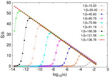
Figure 1: Action $S(\alpha)$ for various parameters $1/\beta$.

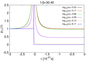
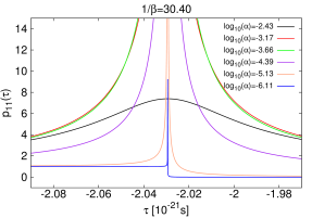
Figure 2: Left panel: Pseudo-occupation of the lower adiabatic level for solutions with various $\alpha$ at fixed $1/\beta=30.40$. The corresponding $S(\alpha)$ is shown in Fig. 1. The pseudocrossing occurs at $\tau_{c}\approx-2.03$. Right panel : The same in greater detail, close to $\tau_{c}$.

For an illustration of non-adiabatic transitions, in Fig. 2 we show the pseudo-occupation $p_{11}(\tau)$ defined in Sect. II B [after the formula (15)]. It is displayed for the same $\alpha$ values which were used to calculate $S(\alpha)$ in Fig. 1, for $1/\beta=30.40$. It can be seen that for $\alpha$ greater than $\alpha_{max}$ ($\log_{10}(\alpha_{max})\approx-3.95$), most of the time $p_{11}$ is concentrated in the lower adiabatic state; a transition to the upper adiabatic state takes place only around the pseudo-crossing, while behind it the system returns to the lower state, i.e. $p_{11}(\tau=0)=1$. This behaviour changes when we approach the maximum of action - for $\log_{10}(\alpha)=-4.39$ - the system behind the crossing remains partially excited to the upper adiabatic level ($0<p_{11}(\tau=0)<1$). For still smaller $\alpha<\alpha_{max}$, behind the pseudo-crossing the system occupies exclusively the upper adiabatic level, till the end of the barrier ($p_{11}(\tau=0)=0$; $p_{21}(\tau=0)=1$). In such a case we have a continuation of the diabatic state.

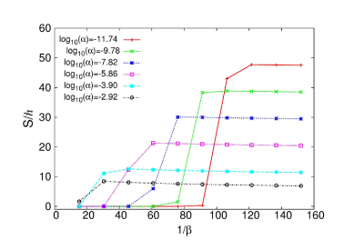
Figure 3: Action $S(1/\beta)$ for various values of $\alpha$.

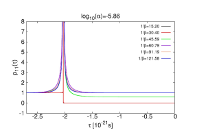
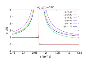
Figure 4: Left panel: Pseudo-occupation of the lower adiabatic level for solutions with various $1/\beta$ at fixed $\log_{10}(\alpha)=-5.86$. The corresponding action $S(1/\beta)$ is shown in Fig. 3. The pseudo-crossing occurs at $\tau_{c}\approx-2.03$. Right panel: The same in greater detail, close to $\tau_{c}$.

In Fig. 3 is shown a plot of action as a function of $1/\beta$ at the fixed $\alpha$, which corresponds to the fixed matrix element $\langle\psi_{1}|\partial_{q}\psi_{2}\rangle$. One can see its jump-like character: for small $1/\beta$ action is close to zero, over a short interval of $1/\beta$ it rises rapidly to a maximal value and then it decreases very slowly. The jump is more sharp and larger for smaller values of $\alpha$, which correspond to a sharper pseudo-crossing between the adiabatic levels. As $1/\beta\sim 1/\Gamma\sim 1/{\dot{q}}_{max}$, the greater the velocity, the stronger the coupling between the adiabatic levels, so for sufficiently large $\dot{q}$ (small $1/\beta$) one can expect a diabatic continuation (transition to an upper adiabatic level) when passing through the pseudo-crossing, which means a small action. One should notice that action vanishing in the limit of very large ${\dot{q}}$ is an artificial property of the model with a finite number of states - after reaching the highest one the system cannot excite anymore.

For smaller ${\dot{q}}$, after passing through the pseudo-crossing, pseudo-occupations of both adiabatic states become comparable - action becomes sizable. For still smaller $\dot{q}$, the pseudo-occupation $p_{21}$ of the upper adiabatic state is non-zero only around the pseudo-crossing, and action does not change much. This also can be seen in Fig. 4 where the pseudo-occupation of the lower adiabatic state is shown for the lower iTDSE solution at the fixed value of $\alpha$. The diabatic behaviour - a sharp fall of $p_{11}$ from 1 to 0 at the pseudo-crossing (red and black lines) - gives way to an intermediate situation - $0<p_{11}<1$ behind pseudo-crossing (green line) - and then to the adiabatic one - $p_{11}=1$ except the close neighbourhood of the pseudocrossing (all other lines). One can notice from Fig. 3 that a smaller $\alpha$ means a larger domain of diabatic behaviour in $1/\beta$, i.e. as $\alpha$ decreases, the interval of a diabatic - to - adiabatic transition shifts towards smaller collective velocities (larger $1/\beta$).

Presented solutions determine whether the evolution is diabatic, intermediate or adiabatic. Since values of $\alpha$ pertinent to nuclear potential with nonaxial deformation can be as small as $\sim 10^{-6}$ - $10^{-7}$, cf Sec. IV.3, this simple model demonstrates a possibility of large variation in action for a fixed $\alpha$, resulting from the dependence on the collective velocity ${\dot{q}}$ at the crossing. As Fig. 1 suggests, even for very small $V$ one can get sizabele action. In a realistic case, with many interacting levels, it is difficult to predict the effect of one pseudo-crossing on the value of action without solving for the instanton-like solution.

Independent of the above results, we have checked that in the adiabatic limit of small ${\dot{q}}/V=\beta/\alpha$, the two-level model produces action which tends to the value given by the formula (65) with the cranking mass parameter, see Piaski .

IV Instanton-like solutions with the Woods-Saxon potential

From this point on, we shall consider instanton-like iTDSE solutions related to the realistic s.p. Woods-Saxon potential within the microscopic-macroscopic framework briefly described below.

Deformation enters the s.p. potential via a definition of the nuclear surface by WS :

$$R(\theta,\varphi) = c(\{\beta\})R_{0}\{1+\sum_{\lambda>1}\beta_{\lambda 0}Y_{\lambda 0}(\theta,\varphi)+$$ (47)

$$\sum_{\lambda>1,\mu>0,even}\beta_{\lambda\mu c}Y^{c}_{\lambda\mu}(\theta,\varphi)\},$$

where $c(\{\beta\})$ is the volume-fixing factor. The real-valued spherical harmonics $Y^{c}_{\lambda\mu}$, with even $\mu>0$, are defined in terms of the usual ones as: $Y^{c}_{\lambda\mu}=(Y_{\lambda\mu}+Y_{\lambda-\mu})/\sqrt{2}$. Here we restrict shapes to reflection-symmetric ones and allow only for the quadrupole non-axiality $\beta_{22}$. The $n_{p}=450$ lowest proton levels and $n_{n}=550$ lowest neutron levels from $N_{max}=19$ lowest major shells of the deformed harmonic oscillator were taken into account in the diagonalization procedure. Eigenenergies are used to calculate the shell- and pairing corrections. The macroscopic part of energy is calculated by using the Yukawa plus exponential model KN . All parameters used here, of the s.p. potential, the pairing strength and the macroscopic energy, are equal to those used previously in the calculations of masses WSparmac ; Qmass and fission barriers Kow ; 2bar ; JKSs ; JKSa of heaviest nuclei, whose results are in reasonable agreement with data. In particular, we took the ”universal set” of potential parameters and the pairing strengths $G_{n}=(17.67-13.11\cdot I)/A$ for neutrons, $G_{p}=(13.40+44.89\cdot I)/A$ for protons ($I=(N-Z)/A$), as adjusted in WSparmac . As always within this model, $N$ neutron and $Z$ proton s.p. levels have been included when solving BCS equations.

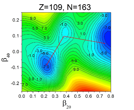
Figure 5: Energy surface of ²⁷²Mt; a chosen trajectory coloured in red.

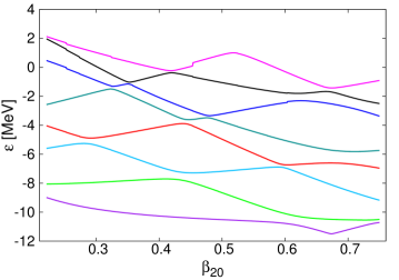
Figure 6: Neutron levels $\Omega^{\pi}=1/2^{+}$ around the Fermi level of ²⁷²Mt along the trajectory shown in Fig. 5.

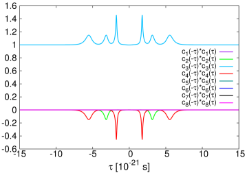
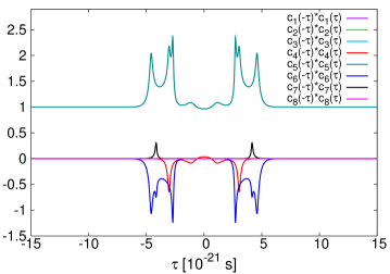
Figure 7: Pseudo-occupations of the adiabatic states for instanton - like iTDSE solutions; upper panel: for $\phi_{3}$, lower panel: for $\phi_{5}$. Colours correspond to the levels of Fig. 6.

First we discuss the iTDSE solutions for axially-symmetric nuclear shapes composed of multipoles with even $\lambda$. In this case the $\tau$-evolution of groups of states with different $\Omega^{\pi}$ are indepedendent of each other. As an example we take 8 neutron $\Omega^{\pi}=1/2^{+}$ states in the W-S potential for ²⁷²Mt along the axially symmetric fission path shown on the energy map in Fig. 5. The map was obtained from the four-dimensional (4D) calculation by minimizing energy of the lowest odd proton and neutron configuration over $\beta_{60},\beta_{80}$ at each $\beta_{20},\beta_{40}$, i.e. without keeping the $K^{\pi}$ configuration of the g.s. Then, to assure a continuity of the path, $\beta_{60}$ and $\beta_{80}$ were chosen continuous and close to those of the minimization, with energy changed by no more than 200-300 keV. Collective velocity was calculated from Eq. (8) by taking the effective (i.e. tangent to the path) cranking mass parameter of the e-e ($Z-1$,$N-1$) nucleus ²⁷⁰Hs. The adiabatic neutron levels in the basis for solving iTDSE were chosen so, that in the g.s. the lower four are occupied (the fourth one singly) and the upper four are empty. In Fig. 6, they are shown along $\beta_{20}$ which, here and in the following, will play a role of the effective collective coordinate $q$ along fission paths.

The method which we used for solving the iTDSE in this and all other cases reported here is described in Appendix B. We find solutions for a finite period $T$ in a finite adiabatic basis and for each of them we calculate action. A natural question then is what would be the limiting values of $S_{i}$ for occupied states when $T\rightarrow\infty$ and the dimension of the basis ${\cal N}\rightarrow\infty$. We tried to answer this by finding actions for increased periods, and by incresing dimension of the adiabatic basis and inspecting the quasi-occupation coefficients. Results of such tests showed that with moderately long periods and rather small bases one can obtain reasonably stable action values for occupied states - see Appendix C.

For the discussed eight levels in ²⁷²Mt, the iTDSE solutions were obtained with the period $T=30\times 10^{-21}$ s. The amplitudes $C_{\mu i}(\tau)$ of solutions have exponential $\tau$-dependence, reach very large values in the interval $[-T/2,0]$ and very small in $[0,T/2]$. It is more informative to characterize solutions by quasi-occupations $p_{\mu i}$ of adiabatic states for selected solutions. This also makes sense from the point of view of action (19) which is built of these quantities. In Fig. 7, quasi-occupations $p_{\mu i}$ are shown for two solutions, $\phi_{3}$ and $\phi_{5}$. It can be seen that at $\tau=\pm T/2$, $p_{\mu i}\cong\delta_{\mu i}$, with minuscule admixtures which should vanish completely for $T=\infty$. During imaginary-time evolution, $p_{\mu i}$ are concentrated on the corresponding adiabatic states $\psi_{\mu=i}$, except around the pseudo-crossings where a partial excitation to the nearest-neighbour state occurs. Until a pseudo-crossing is isolated (there is no other pseudo-crossing nearby) excitations to other states are negligible. If successive pseudo-crossings follow one after another, the quasi-occupations of other adiabatic levels are possible, as seen for the solution $\phi_{5}$ which locally becomes a combination of $\psi_{6}$ and $\psi_{7}$, and then of $\psi_{4}$ and $\psi_{6}$ - see Fig. 7.

Next we discuss some properties of iTDSE solutions which seem relevant for their physical interpretation and applications.

IV.1 Rise of action with the collective velocity $\dot{q}$

With cranking mass parameters fixed along a path, the collective velocity of tunneling is proportional to $\sqrt{E(q)-E_{0}}$, where $E(q)-E_{0}$ is a plot of the fission barrier (reduced by $E_{zp}$). In a selfconsistent instanton calculation, the increase in barrier height also relates to an increase in the magnitude of ${\dot{q}}$ necessary to increase the difference between $|\Phi(\tau)\rangle$ and $|\Phi(-\tau)\rangle$ in order to keep their energy overlap ${\cal H}(\tau)$ constant. On the other hand, in our non-selfconsistent treatment, ${\dot{\beta}}_{20}$, i.e. our ${\dot{q}}(\tau)$, is simply an assumed functional parameter of the solution to Eq. (12). However, having in mind its implied physical relation to the barrier height, we tested the action dependence on $|{\dot{\beta}}_{20}|$. The collective velocity for ²⁷²Mt determined from (8) with the cranking mass parameter from the neighbouring e-e nucleus (Z=108, N=168) along the path depicted in Fig. 5 is shown in Fig. 8. This profile was then scaled by the factors 1.3 and 1.6. The action calculated for all occupied neutron states of positive parity for three collective velocities is given in Table 1.

Figure 8: Collective velocity ${\dot{q}}$ in units od $10^{21}$ s^-1 calculated from (8) for ²⁷²Mt along the path shown in Fig. 5.

One can see that action indeed increases with $|{\dot{q}}|$, as the expected relation with the barrier height would suggest. Detailed outcome is dependent on the s.p. level scheme, in particular, pseudocrossings close to the Fermi level. In Eq. (12), the coupling terms causing non-adiabatic transitions are $\dot{q}\langle\psi_{i}|\partial_{q}\psi_{j}\rangle$, so the main influence on $S$ have regions in $q$ where a large $|\dot{q}|$ occurs at a sharp pseudocrossing.

Collective velocity	$S_{tot}=\sum_{\Omega^{+}}S_{\Omega^{+}}$ $[\hbar]$
$\dot{q}$	21.3465
$1.3\,\dot{q}$	24.6362
$1.6\,\dot{q}$	28.6790

Table 1: Action $S_{tot}$ for neutron states of positive parity in ²⁷²Mt as a function of scaled collective velocity. The profile $\dot{q}$ corresponds to the formula (8) for the path in Fig. 5.

IV.2 Integrand of action vs mass parameters

One can ask whether it would be possible to define a mass parameter $B(q)$ from the $\tau$- even action integrand in Eq. (19) by:

$$\sum\limits_{i,occ}\sum\limits_{\mu=1}^{\cal N}[\zeta_{i}-\epsilon_{\mu}(q(\tau))]p_{\mu i}(\tau)=B_{qq}(q)\dot{q}^{2}.$$ (48)

In Fig. 9 are shown contributions to the integrand of action from s.p. bounce-like states and their sum for even and odd number of particles (19). Calculations were done for the same $\Omega^{\pi}=1/2^{+}$ neutron states in ²⁷²Mt, for a path shown in Fig. 5. It can be seen that while integrands of single iTDSE solutions sometimes show a rather complicated pattern, their sum is much more regular. This comes from a cancellation of excitations among solutions corresponding to occupied levels and only excitations to levels above the Fermi level count. There is no drastic difference between the even- and odd-particle-number case - it is just a contribution from one singly occupied instanton-like solution, which may be both positive or negative in general. This is in contrast to the cranking approach, where for the odd-$A$ case, mass parameter (I) and the action integrand (1) would show large peaks at pseudocrossings of the unpaired level.

As seen in Fig. 9, the integrand (48) becomes negative around the endpoints $\tau\rightarrow\pm T/2$, so it cannot define any mass parameter. This follows from differences between the Floquet exponents $\zeta_{i}$ and s.p. energies $\epsilon_{i}$ at the g.s. minimum, which, as stated in Sect. II.2, is the artefact of using $T<\infty$ in practical calculation. The same difficulty will probably remain in the selfconsitent calculations.

However, even for a positive integrand of action there would be a more general impediment to deriving the mass parameter. The beyond-cranking treatment means that the integrand of action depends on all even powers of $\dot{q}$. Thus, for a given path, $B_{qq}$ of (48) would be dependent on $|{\dot{q}}|$.

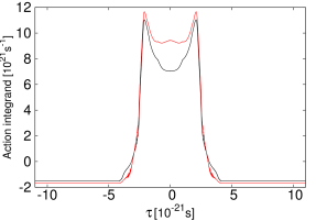
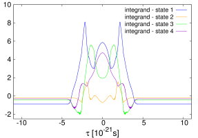
Figure 9: Left: The total action integrand in units $10^{21}$ s^-1 - the sum of individual contributions - for six (in black) and seven (in red) neutrons - taken from Piaski . Right: Contributions to the integrand of action from individual s.p. solutions.

On the other hand, since a solution along the prescribed path depends on it, two different paths tangent at a common point ${\bf q}$ (what would imply eqal effective cranking mass parameters at ${\bf q}$) would have generally different integrands of action at ${\bf q}$.

IV.3 Calculations along nonaxial path for neutron states in ²⁷²Mt

A solution of iTDSE equations for nonaxial shapes turns out to be more difficult than in the case of axial deformations considered hitherto. The W-S spectrum along a nonaxial fission path shows many sharp pseudocrossings between levels of the same parity, some with interaction as small as $V\sim 10^{-5}-10^{-6}$ MeV (see Fig. 10). Although for $V\rightarrow 0$ such levels would cross, the results for the two-level model have shown (Sec. III) that this limit is subtle and depends also on the collective velocity and the slopes of crossing levels. It happens that diabatic continuation, i.e. assuming $V\approx 0$, may lead to large errors in calculated action. On the other hand, many pseudo-crossings with a very weak interaction, leading to extremely high peaks in the matrix elements which couple involved adiabatic states, are the obstacle in solving iTDSE. The encountered problem and its (rather cumbersome) solution are described below.

Calculations were performed along the chosen nonaxial path for ²⁷²Mt, see Fig. 10, for ${\cal N}=32$ neutron states of positive parity. In the first version, we used the data from the W-S code along the path with a variable step, not shorter than $\Delta\beta_{20}=10^{-6}$. In the second version, the minimal step was smaller, $\Delta\beta_{20}=10^{-7}$. Finally, in the third version, we used the procedure described in the Appendix D, with the minimal step $\Delta\beta_{20}=10^{-7}$, and the analytic model (73) adjusted to those peaks for which the minimal stepsize still did not cover their range with a sufficient precision. Actions calculated for occupied instanton levels and their sum are given in Table 2. It can be seen that actions for some individual levels in the first and second versions of the calculation differ widely - this means that the step $\Delta\beta_{20}=10^{-6}$ is not sufficient. This is consistent with an insufficient density of points for a description of particular pseudocrossings, as revealed by the inspection of related coupling matrix elements. In spite of this, the total action is similar in two versions of calculation. This is yet another sign that action depends on pseudo - crossings close to the Fermi levels - the details of crossings far above or below the Fermi energy (between both occupied or both unoccupied levels) do not have effect on total action.

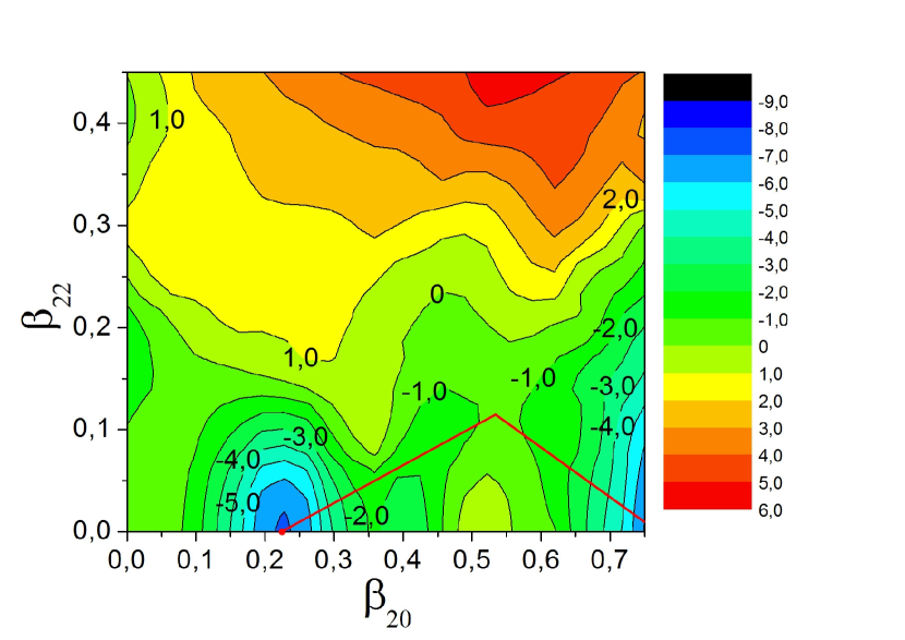
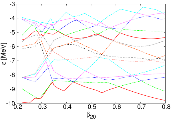
Figure 10: Left: Energy landscape for ²⁷²Mt in $\beta_{20}-\beta_{22}$, minimized over $\beta_{40},\beta_{60},\beta_{80}$ with a chosen fission path (marked in red). Right: Display of 14 positive-parity neutron levels around the Fermi energy along the fission path; the 7-th level from below is the last occupied.

In the third version of the calculation, the highest peaks in the coupling matrix elements were replaced by the peaks modelled analytically (73). Actions obtained within this method (in the third column in Table 2), both for individual solutions and the total, are close to those of the second version. This is probably related to the fact that difficult couplings that were modelled occur at such $q$, where $\dot{q}\approx 0$, so that they were suppresed in the instanton equations (12). In general, however, the procedure of peaks modelling seems indispensable for obtaining sufficiently exact actions if the instanton equations are to be solved in the adiabatic basis (in particular, when a very large nonadiabatic coupling occurs close to the Fermi energy).

Nr	$\Delta\beta_{20}=10^{-6}$	$\Delta\beta_{20}=10^{-7}$	$\Delta\beta_{20}=10^{-7}$ plus fit
1	3.2143	3.2057	3.1936
2	0.9453	8.0320	8.0555
3	3.2931	6.9294	6.9118
4	3.2790	-8.7864	-8.7867
5	-0.0346	2.1493	2.1684
6	-1.7771	-2.3285	-2.3531
7	0.9953	1.1126	1.1129
8	8.8511	9.1817	9.1458
9	4.1217	-1.3617	-1.4455
10	5.5588	9.6487	9.8299
11	-2.9214	-2.3793	-2.3817
12	-4.5752	-4.5158	-4.5660
13	-0.4160	-0.3668	-0.3788
14	6.7950	6.4864	6.4848
15	6.6443	6.4057	6.4033
16	2.8743	2.8123	2.8128
$\mathbf{S_{tot}/\hbar}$	36.8479	36.2254	36.2069

Table 2: Actions for separate s.p. solutions occupied at the g.s. and their sum - the total action for a nonaxial path; first column: calculations with the minimal step $\Delta\beta_{20}=10^{-6}$; second column: calculations with the minimal step $\Delta\beta_{20}=10^{-7}$; third column: calculations with the minimal step $\Delta\beta_{20}=10^{-7}$ augmented with the modelling of the highest peaks in the nonadiabatic couplings by the formula (73).

We also checked the dependence of action on the dimension ${\cal N}$ of the adiabatic basis. We changed ${\cal N}$ from 14 to 32, always keeping the Fermi level at ${\cal N}/2$ (as in Appendix C.2 for the axially symmetric path). The results given in Tab. 3 indicate that the dominant contribution to action comes from levels around the Fermi level.

Action obtained for the trajectory along nonaxial shapes was compared to the one along the axially symmetric path (shown in Fig. 5) in Table 4. In both cases the same neutron levels with positive parity were included. It can be seen that action along the shorter, axially symmetric path is smaller in spite of the fact that the barrier is lower by $\sim 2$ MeV along the nonaxial path, what in our treatment translates into a smaller collective velocity ${\dot{q}}$.

It has to be emphasized that the last result cannot be treated as general - it merely shows that the instanton method applied to reasonably chosen paths can lead to situations similar as in calculations with the cranking mass parameters. Deciding whether axial or nonaxial path prevails would require a minimization procedure not defined here.

${\cal N}$	$S_{tot}=\sum_{i=1}^{{\cal N}/2}S_{i}$ $[\hbar]$
16	27.0313
20	35.8289
24	35.9705
28	36.1187
32	36.2069

Table 3: Action (in $\hbar$) for neutrons of positive parity along the nonaxial path for various numbers ${\cal N}$ of included adiabatic states.

Path	$B_{f}$ [MeV]	$S_{tot}/\hbar$
axial	8.4	21.35
nonaxial	6.5	36.21

Table 4: Fission barrier heights $B_{f}$ and actions $S_{tot}$ (in $\hbar$) for neutrons of positive parity in ²⁷²Mt along the axial (Fig. 5) and nonaxial (Fig. 10) fission paths.

V Fission hindrance in odd nuclei - a study

Usually, the spontaneous fission hindrance factors $HF$ for odd nuclei are defined as $T_{sf}^{o}/T_{sf}^{ee}$, where $T_{sf}^{o}$ is the spontaneous fission half-life of an odd nucleus and $T_{sf}^{ee}$ is a geometric mean of the fission half-lives of its e-e neighbours Hess . Experimental facts are that 1) most of $HF$ values lie between $10^{3}$ to $10^{5}$, 2) they do not display any strong dependence on the $K(=\Omega)$ quantum number of the g.s. configuration Hess .

Here, we will use $HF$ calculated as:

$$HF=\frac{T_{sf}^{o}}{T_{sf}^{e}},$$ (49)

where $T_{sf}^{o}$ i $T_{sf}^{e}$ are fission half-lives of an odd-A nucleus and its $A-1$ e-e neighbour.

Experimental fission half-lives and odd-even $HF$s can be converted into relations between actions for odd-$A$ and e-e neighbours by using the $WKB$-motivated formula for spontaneous fission half-lives:

$$\log_{10}(T_{sf}[s])=-20.54+0.8686\,\frac{S}{\hbar}-\log_{10}\left(\frac{E_{zp}}{0.5\>MeV}\right).$$ (50)

Here, $S$ is the minimal action chosen among all possible fission paths, and $E_{zp}$ is the zero-point energy (in MeV) of vibration along the fission direction around the m.s. Assuming a universal value of $E_{zp}$, which is surely an approximation, one obtains:

$$\log_{10}(HF)\approx 0.8686\ \frac{S_{odd}-S_{even}}{\hbar}.$$ (51)

Calculations were performend for selected superheavy nuclei with known half-lives and, in some cases, known g.s. spin and parities, indicating possible configurations. A similar calculations for actinide nuclei would be much more involved in view of their much longer and more complex barriers.

V.1 Instanton-like action without pairing for ²⁵⁷Rf, ²⁵⁷Rf

By solving iTDSE for a given path and collective velocity profile ${\dot{q}}(\tau)$ one can calculate action for both even and odd nuclei, neglecting pairing. Such results would correspond to a scenario originally put forward by Hill and Wheeler HillWhee . Without pairing they cannot be realistic, but allow to notice a few things, among them how much fission would be hindered without pair correlations.

We choose the odd nucleus ²⁵⁷Rf as the example. Its $I^{\pi}=1/2^{+}$ g.s., which well corresponds to the $K^{\pi}=\Omega^{\pi}=1/2^{+}$ configuration in the W-S model, has a known spontaneous fission half-life of $T_{sf}^{odd}=423$ s Hess . Also known is the experimental lower limit of $T_{sf}^{odd}>490$ s Hess for the half-life of the excited $I^{\pi}=11/2^{-}$ state, corresponding to the $K^{\pi}=11/2^{-}$ configuration in our micro-macro model. The experimental spontaneous fission half-life for the e-e neighbour ²⁵⁶Rf is $T_{sf}^{even}=6.4$ ms Hess , which gives $HF=6.6\times 10^{4}$ (for $K^{\pi}=1/2^{+}$ configuration) and $HF>7.6\times 10^{4}$ (for $K^{\pi}=11/2^{-}$).

The tunneling path was chosen as follows. First, micro-macro energy landscapes of two nuclei were calculated by using mass-symmetric axial deformations: for each $\beta_{20}-\beta_{40}$ energy was minimized over $\beta_{60},\beta_{80}$, with the steps $\Delta\beta_{20}=0.05$ and $\Delta\beta_{40}=0.025$. The odd nucleus configurations $K^{\pi}$ were kept constrained at $K^{\pi}=1/2^{+}$ and $K^{\pi}=11/2^{-}$ for the g.s. and the excited state, respectively. This means a continuation, possibly non-adiabatic, of the state $\Omega^{\pi}$ occupied by the odd neutron at the energy minimum. A similar calculation, but without blocking, was performed for ²⁵⁶Rf. It can be seen from the maps in Fig. 11 that keeping the configuration in the odd nucleus leads to a substantial increase and elongation of the barrier, especially for the excited configuration $K^{\pi}=11/2^{-}$. Taking into account the experience from action minimization calculations, the fission path was chosen piecewise straight and close as possible to the minimal energy, in order to keep the path short and the barrier low (the path is also piecewise straight in $\beta_{60},\beta_{80}$). It is depicted in red in Fig. 11

Instanton-like action $S_{inst}$ was calculated by solving iTDSE with the collective velocity: ${\dot{q}}_{P}=\sqrt{2(E(q)-E_{m.s.})/B_{P}(q)}$, where $E(q)-E_{m.s.}$ is deformation energy with respect to the m.s. for each nucleus/configuration (i.e. with $E_{zp}$ set to zero), and $B_{P}(q)$ is the cranking mass parameter of ²⁵⁶Rf, both including pairing and calculated along the chosen paths. So, strictly speaking, ${\dot{q}}_{P}$ derives from the paired system, but iTDSE is solved for the system without pairing. For comparison, along the same paths we calculated actions:

$$S_{cr}({\dot{q}}_{P})=\int_{-T/2}^{T/2}d\tau\,B_{NP}(q)\,\dot{q}_{P}^{2},$$ (52)

with the same ${\dot{q}}_{P}(\tau)$ and the cranking mass parameter $B_{NP}(q)$ without pairing for each nucleus (i.e. also for the odd one). The mass parameter $B_{NP}$ includes large peaks due to close avoided level crossings which should considerably increase action relative to $S_{inst}$. We can calculate action $S_{cr}({\dot{q}}_{P})$ accurately thanks to the large number of points - few thousands per path. Both actions are given in Table 5.

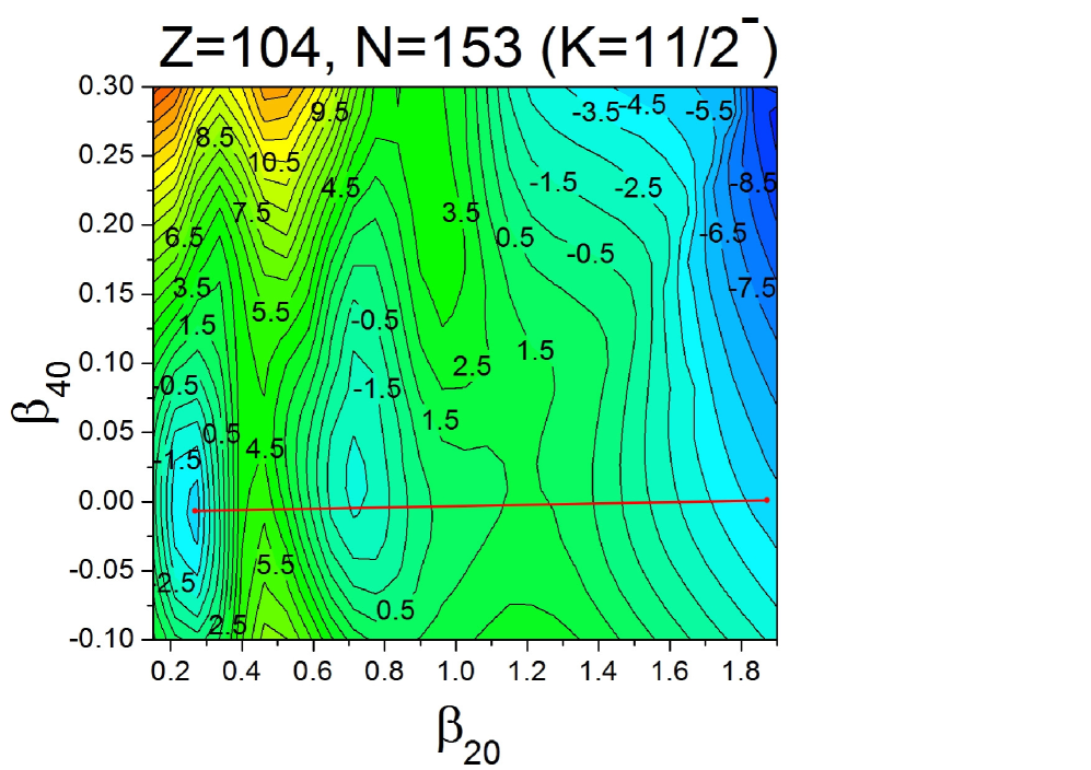
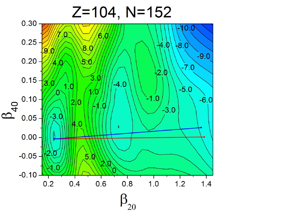
Figure 11: Upper panel: energy landscapes for ²⁵⁷Rf minimized over $\beta_{60},\beta_{80}$ with fixed $K^{\pi}=1/2^{+}$ (left) and $K^{\pi}=11/2^{-}$ (right) configuration. Lower panel: energy landscape for the neighbouring ²⁵⁶Rf. Chosen fission paths marked in red. For e-e ²⁵⁶Rf also a second path (marked in blue) was considered (see text). Note different ranges of $\beta_{20}$ in maps.

Nucleus ($K^{\pi}$)	257Rf ($1/2^{+}$)		257Rf ($11/2^{-}$)		256Rf
Action [$\hbar$]	$S_{inst}$	$S_{cr}({\dot{q}}_{P})$	$S_{inst}$	$S_{cr}({\dot{q}}_{P})$	$S_{inst}$	$S_{cr}({\dot{q}}_{P})$
Neutrons ($+$)	27.29	86.40	31.23	68.41	19.52	32.11
Neutrons ($-$)	73.71	1378.97	82.06	1539.65	65.53	1172.65
Protons ($+$)	46.19	9530.25	50.46	9754.98	46.09	9393.87
Protons ($-$)	15.34	21.76	19.11	46.94	12.87	16.39
Sum	162.53	11017.38	182.86	11409.98	144.01	10615.02

Table 5: Actions (in $\hbar$) for ²⁵⁶Rf and both configurations in ²⁵⁷Rf obtained with collective velocities ${\dot{q}}_{P}$ (see text) along paths shown in Fig. 11: instanton-like $S_{inst}$ and with the cranking mass parameter without pairing - $S_{cr}({\dot{q}}_{P})$. Contributions from neutrons and protons of each parity (indicated in parentheses) are given separately.

We also calculated cranking action without pairing $S_{crank}$, i.e. twice the expression of Eq. (1) with the integrand $\sqrt{2B_{NP}(q)(E(q)-E_{m.s.})}$, i.e. with the mass parameter $B_{NP}(q)$ and collective velocity ${\dot{q}}_{NP}=\sqrt{2(E(q)-E_{m.s.})/B_{NP}(q)}$.

As might be expected, $S_{cr}({\dot{q}}_{P})$ hugely overestimates $S_{inst}$ - nearly by two orders of magnitude (Tab. 5), mainly because of pseudo - crossings of s.p. levels close to the Fermi energy. Locally, around them, $B_{NP}>>B_{P}$, and this results in large local contributions to action $S_{cr}({\dot{q}}_{P})$. The local bumps in $B_{NP}$, capriciously dependent on details of avoided level crossings, explain vastly different contributions to $S_{cr}({\dot{q}}_{P})$ from different groups of levels: $\sim 90$% of $S_{cr}({\dot{q}}_{P})$ comes from protons of positive parity, while the contributions from protons of negative parity in ²⁵⁶Rf and 1/2⁺ state in ²⁵⁷Rf are similar as those to $S_{inst}$ (Tab. 5). Using $\dot{q}_{NP}$, which differs from ${\dot{q}}_{P}$ mainly in that it is much smaller at pseudo-crossings, largely reduces action: one obtains $S_{crank}=199.28\,\hbar$ for ²⁵⁶Rf and $222.48\,\hbar$ for ²⁵⁷Rf ($K^{\pi}=1/2^{+}$), results larger than, but much closer to instanton-like action $S_{inst}$.

From (50), after assuming $E_{zp}=0.5$ MeV, we obtain ”experimental” actions of $2S=42.24\ \hbar$ for ²⁵⁶Rf and $2S=53.34\ \hbar$ for the g.s. of ²⁵⁷Rf - these doubled actions should be compared to values from Tab. 5. Thus, calculated $S_{inst}$ are $\approx 3.5$ times bigger than the values following from measured half-lives.

We have checked that the instanton action calculated according to the given prescription very much depends on the path. For the trajectory coloured in blue in Fig. 11, we obtained for ²⁵⁶Rf $S_{inst}({\dot{q}}_{P})=167\ \hbar$, larger by 23 $\hbar$ than for the not very different red one. Apparently, in the absence of pairing, the details of pseudo - crossings have large influence on action. This shows that action minimization without pairing might be very difficult and would be directing into paths with more gentle crossings.

The difference between instanton-like actions $S_{odd}$ and $S_{even}$ comes from: 1) a collective contribution - from the differences in deformation energy of the e-e and odd-$A$ nuclei, which in turn comes from: a) different collective velocities and b) different lengths of the path; 2) a contribution to action from the odd nucleon foot3 .

Note that in the instanton method without pairing, the odd - even effect in fission half-lives comes exclusively from different heights and lengths of the fission barriers. If not for these, action for odd-$A$ would lie between those of neighbouring $A-1$ and $A+1$ e-e species, as it is a sum of individual s.p. instanton-like actions, Eq. (19).

For two configurations in ²⁵⁷Rf we have from Tab. 5: $\Delta S_{odd-even}=18.52\;\hbar$ for $K^{\pi}=1/2^{+}$, and $\Delta S_{odd-even}=38.85\;\hbar$ for $K^{\pi}=11/2^{-}$. This large difference of $20.33\;\hbar$ can be traced to a larger ${\dot{q}}_{P}$ for the second configuration, and could be predicted from their very different barriers in Fig. 11. This well illustrates the trend towards higher barriers in calculations with a fixed-$K$ configurations, and those with higher $K$ values in particular. Such $K$-dependence is absent in experimental half-lives (see Fig. 17 in Hess ).

We note that for the relative quantities, $\Delta S_{odd-even}/S_{odd}$, for the g.s. of ²⁵⁷Rf and ²⁵⁶Rf we obtain from (50), again assuming the same $E_{zp}$, the ratio 0.114 vs. the experimental value 0.21. However, the minimization of action, not attempted here, could change this ratio.

V.2 Calculations assuming collective mass parameter and an odd - particle contribution

Without having solved Eq. (31) with pairing, we will use unpaired iTDSE solutions to study odd-even fission hindrance by adopting a hybrid model which incorporates both pairing and the odd particle contribution to action.

We assume the following scheme. Action for an e-e nucleus is taken from Eq. (1) with both energy and the cranking mass parameter including pairing. For an odd-$A$ nucleus we assume:

$$S_{odd}=S_{crank}+\frac{1}{2}S_{s.p.}^{inst}\;,$$ (53)

where $S_{crank}$ is the cranking action (1) of the e-e core, calculated with the micro-macro barrier for the odd-$A$ nucleus, $E^{odd}(q)-E_{0}$, where $E_{0}=E_{m.s.}+E_{zp}$, and the cranking mass parameter with pairing $B^{even}_{P}(q)$ of the neighbouring e-e $A-1$ system, while $S_{s.p.}^{inst}$ is the contribution to action from the unpaired nucleon. It can be calculated as action of the instanton-like solution corresponding to the unpaired $\Omega^{\pi}$ state (i.e. the one blocked in the m.s.) with the collective velocity ${\dot{q}}_{P}=\sqrt{2(E^{odd}(q)-E_{m.s.})/B^{even}_{P}(q)}$, or as the difference in actions for occupied $\Omega^{\pi}$ states between the odd-$A$ and e-e $A-1$ nucleus. Both ways of calculating $S_{s.p.}^{inst}$ give very similar values; we will give those by the second method. The factor $1/2$ in (53) accounts for the fact that $S_{inst}$ corresponds to twice action of Eq. (1).

The rationale behind the choice of the mass parameter and, consequently, of the collective velocity ${\dot{q}}_{P}$, is the assumed collectivity of quantum tunneling in spontaneous fission. We reject the cranking mass parameter for odd-$A$, Eq. (I), as it leads to huge differences between collective velocities ${\dot{q}}$ at the neighbouring $q$ points in an odd-$A$ nucleus, and between $A$ and $A-1$ nuclei at the same $q$ point. Outside regions where pseudo-crossings of the odd level take place, the cranking mass parameters for $A$ and $A-1$ nuclei are similar, see Eq. (I). Thus, eliminating huge variations from the mass parameter for odd-$A$ is consistent with assuming its magnitude similar as in the even-$A-1$ system, uniformly in $q$. Certainly, similar does not mean equal. However, lack of arguments for any definite ratio singles out the made choice as the simplest one. It means that the difference in actions for $A$ and $A-1$ systems comes mainly from different deformation energies. A choice of the same, or of the same phenomenological formula for, mass parameters for odd-$A$ and e-e $A-1$ nuclei was made in the past Molpar ; LojewF . The results of the previous subsection also point out that such a choice is reasonable. The quantity $S_{s.p.}^{inst}$ is the remaining difference between actions for odd-$A$ and e-e $A-1$ nucleus, coming from the unpaired odd particle.

As examples of the previous subsection indicate, the important point is whether deformation energy of an odd-$A$ nucleus is calculated conserving the configuration $\Omega^{\pi}$ of the g.s. or releasing this requirement and taking the minimal energy among various configurations at each deformation. We performed calculations within our model in both ways in order to compare results.

Included deformation parameters and the choice of fission paths were as discussed in the previous subsection. We selected nuclei $Z=103-112$ for which their, and their even-$A-1$ neighbours fission half-lives are known, and so is the hindrance factor (49). For most of them their g.s. spins and parities are either known or attributed on the basis of phenomenological models Hess .

In Fig. 12, the calculated energy surfaces are shown for ²⁶¹Db and its e-e neighbour ²⁶⁰Rf. The g.s. configuration of ²⁶¹Db is $K^{\pi}=9/2^{+}$. Both surfaces for ²⁶¹Db, adiabatic (minimized over configurations) and constrained on the $K^{\pi}$ value, are given together with chosen fission paths. It can be seen that the fission barriers are double-humped, with a smaller second hump. A similar picture holds for other considered nuclei. A clear difference between adiabatic and $K^{\pi}$ - conserved surfaces can be observed for $K=9/2$ in ²⁶¹Db - one can notice higher and longer second barrier. For smaller $K$, like e.g. the $K^{\pi}=1/2^{+}$ configuration in ²⁵⁹Sg (not shown here), this difference is smaller. A large difference in barriers for high-$K$ configuration was also seen for ²⁵⁷Rf in Fig. 11.

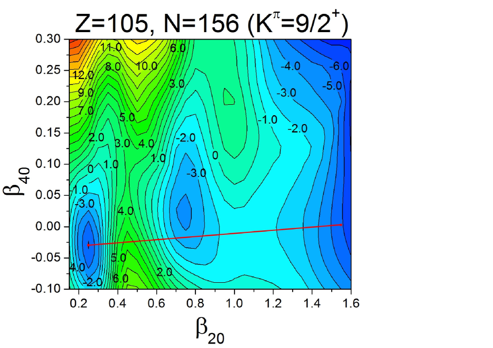
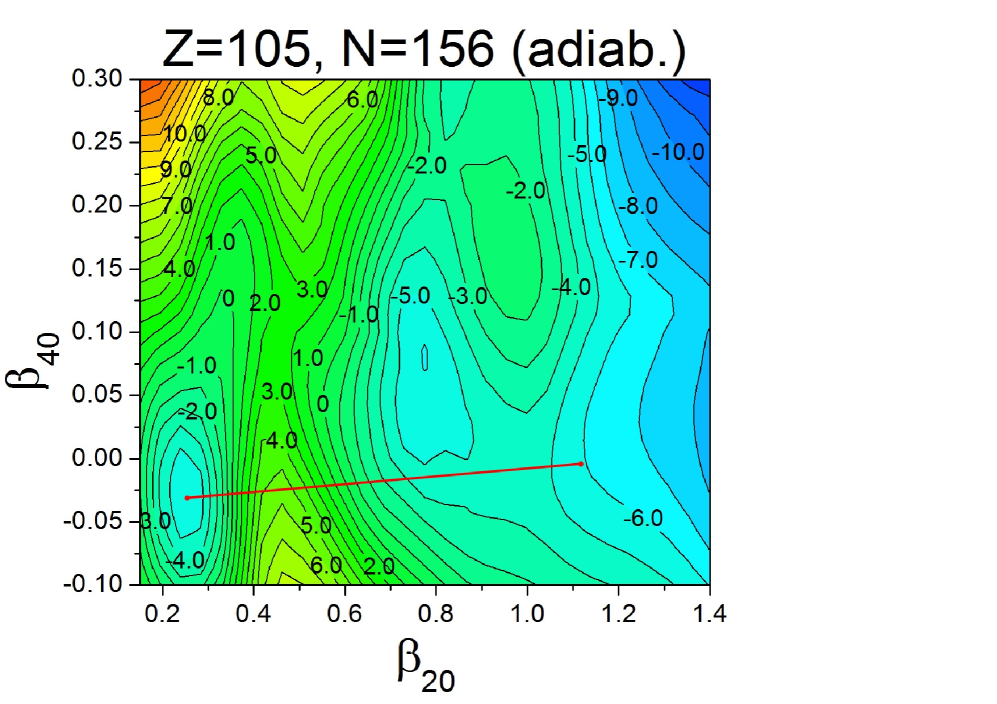
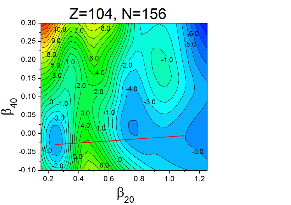
Figure 12: Upper panel: energy landscapes for ²⁶¹Db, minimized over $\beta_{60},\beta_{80}$ with the kept g.s. configuration $K^{\pi}=9/2^{+}$ (left) and adiabatic (right). Lower panel: energy landscape for ²⁶⁰Rf. Chosen fission path marked in red. Note different range of $\beta_{20}$ in maps.

At this point one has to note that our calculations do not include nonaxial deformations, $\beta_{22}$, etc, which lower the first barrier, neither do they account for mass asymmetric deformations lowering the second barrier. Calculations which include nonaxiality indicate that a path through the nonaxial saddle, lower by 1-2 MeV, has a substantially greater length which moderates or even compensates the effect of the lower saddle. On the other hand, the mass asymmetry is lowering the second barrier and the path incorporating it is not much longer (in terms of $ds=\sqrt{\sum_{\lambda\mu}(d\beta_{\lambda\mu}/d\beta_{20})^{2}}d\beta_{20}$) than the one considered here because the mass-asymmetric exit from the barrier occurs for smaller $\beta_{20}$ - thus the effect of $\beta_{\lambda 0}$ with odd $\lambda$ is likely to decrease the action.

It turns out that with realistic values of $E_{zp}$ around 0.5 - 1 MeV we obtain too large actions and half-lives for e-e nuclei as compared to the experimental values. The reason lies in a too limited choice of nuclear shapes and in a relatively small strength of the pairing interaction, dictated by the local mass fit WSparmac . Indeed, we have checked for ²⁵⁶Rf, that with the pairing strengths and $E_{zp}=0.7$ MeV used in sss95 and ignoring the second barrier hump (which is largely reduced by the mass-asymmetry) we reproduce the result reported there which is in good agreement with the experimental value.

Nucleus	$S_{crank}/\hbar$	$T_{sf}^{exp}$ [s]	$T_{sf}^{calc}$ [s]
258No	21.60	1.2E-03	4.1E-03
254Rf	18.46	2.3E-05	7.8E-06
256Rf	21.91	6.4E-03	7.6E-03
260Rf	22.97	2.2E-02	6.4E-02
258Sg	21.92	2.6E-03	7.7E-03
260Sg	23.62	7.0E-03	2.4E-01
282Cn	18.82	9.1E-04	1.6E-05

Table 6: Calculated actions (in $\hbar$) and calculated vs experimental fission half-lives (in seconds) for e-e nuclei after adjusting zero-point energy $E_{zp}$ to minimize the root-mean-square error.

Nucleus	$K^{\pi}$	$S^{conf}_{crank}/\hbar$	$T_{sf}^{crank}$ [s]	$S^{ad}_{crank}/\hbar$	$\Delta S_{crank}/\hbar$
259Lr	7/2-	33.32	6.2E+07	23.44	9.88
255Rf	9/2-	56.06	3.5E+27	25.31	30.75
257Rf	1/2+	34.32	4.6E+08	22.58	11.74
257Rf (m)	11/2-	48.89	2.1E+21	22.58	26.31
261Db	9/2+	40.79	1.9E+14	26.65	14.14
259Sg	1/2+	32.44	1.1E+07	23.23	9.21
261Sg	3/2+	30.75	3.6E+05	25.30	5.45
283Cn	5/2+	24.52	1.4E+00	21.56	2.96

Table 7: For odd nuclei and their $K^{\pi}$ configurations shown in columns 1 and 2 are given cranking actions (1) calculated with the mass parameters of the e-e neighbour: for a fixed $K^{\pi}$ configuration $S^{conf}_{crank}$ (col. 3), for adiabatic configuration $S^{ad}_{crank}$ (col. 5), their difference $\Delta S_{crank}$ (col. 6), all in $\hbar$; half-lives $T_{sf}^{crank}$ (in s) resulting from $S^{conf}_{crank}$ are given in col. 4. The zero point energy $E_{zp}$ was adjusted to experimental fission half-lives of e-e nuclei.

Since we focus here on fission hindrance for odd-$A$ nuclei we decided to artificially change zero-vibration energy $E_{zp}$ so that the mean - square deviation of fission half-lives in e-e nuclei from experimental values is minimal. This happens for $E_{zp}=2.03$ MeV. The fission half-lives of e-e nuclei obtained with the adjusted $E_{zp}$, which will serve as the reference for the calculation of fission hindrance factors in odd-$A$ nuclei, are given in Table 6. They are mostly of the same order of magnitude as the experimental ones, except in ²⁶⁰Sg and ²⁸²Cn. The effect of higher $E_{zp}$ cancels the contribution to action from the second barrier for $Z=102-106$. This is roughly consistent with the results of sss95 , where the barrier was practically reduced to the first hump.

In Table 7 we compare actions $S_{crank}$ of (53) obtained in two ways for odd nuclei: $S_{crank}^{conf}$ - by keeping the fixed configuration, and $S_{crank}^{ad}$ - by using adiabatic occupation of the odd nucleon. Differences between these actions, $S_{crank}^{conf}-S_{crank}^{ad}$, are greater than 9 $\hbar$, except for ²⁶¹Sg and ²⁸³Cn. As we have checked, they remain large for a wide choice of adopted $E_{zp}$ values between 0.5 and 2 MeV. As for e-e nuclei, paths on the adiabatic surfaces effectively do not show the second barrier. With the preserved $K^{\pi}$ configuration, the contribution of the second barrier to action is substantial and strongly dependent on the magnitude of $K$. Fission half-lives calculated with keeping the $K^{\pi}$ configuration, also given in Table 7, vastly overestimate the experimental values (see col. 3 of Table 8 for comparison), except in ²⁸³Cn, with the largest discrepancy for large $K$. Therefore, we do not include odd-particle actions $S_{s.p.}^{inst}$ for them.

Nucleus data				Adiabatic blocking
${}^{A}X$	$I^{\pi}$	$T_{sf}^{exp}$ [s]	$HF_{exp}$	$S_{s.p.}^{inst}/\hbar$	$T_{sf}^{cr}$ [s]	$T_{sf}^{cr+inst}$ [s]	$HF_{calc}^{cr}$	$HF_{calc}^{cr+inst}$
259Lr	7/2-	27.4	2.3E+04	1.02	0.16	0.45	3.9E+01	1.1E+02
255Rf	9/2-	3.15	1.4E+05	-1.37	6.83	1.73	8.8E+05	2.2E+05
257Rf	1/2+	423	6.6E+04	2.43	0.03	0.33	3.9E+00	4.34E+01
257Rf (m)	11/2-	$>$490	$>$76562.5	0.03	0.03	0.03	3.9E+00	3.9E+00
261Db	9/2+	5.6	2.5E+02	0.04	99.6	103.6	1.56E+03	1.62E+03
259Sg	1/2+	8	3.1E+03	1.85	0.11	0.68	1.43E+01	8.83E+01
261Sg	3/2+	31	4.4E+03	0.61	6.7	12.32	2.79E+01	5.13E+01
283Cn	5/2+ (*)	24	2.6E+04	2.76	0.0038	0.06	2.38E+02	3.75E+03

Table 8: For seven odd-$A$ nuclei listed in the first column are given: configurations $I^{\pi}$ (experimental or from systematics), experimental spontaneous fission half-lives $T^{exp}_{sf}$ (after Hess ) and fission hindrance factors $HF_{exp}$ according to (49), and calculated quantities (for the g.s. or m.s. configurations $K^{\pi}=I^{\pi}$): the odd nucleon instanton contribution to action $S^{inst}_{s.p.}$, fission half-lives and $HF$s following from the adiabatic actions $S^{ad}_{crank}$ for the e-e core (given in Tab. 7) and the same augmented with $S^{inst}_{s.p.}$, $S_{crank}^{ad}+\frac{1}{2}S_{s.p.}^{inst}$. Half-lives are given in seconds, actions in units of $\hbar$. Asterisk for ²⁸³Cn signals that the given $T^{exp}_{sf}$ is the smaller of two conflicting experimental values and spin/parity is derived from our W-S spectrum. The symbol (m) denotes the excited configuration.

Results pertaining to half-lives of odd-$A$ nuclei and fission hindrance factors obtained with the adiabatic blocking are given in Table 8 and shown in Fig. 13. Here we include results obtained with $S_{crank}^{ad}$ alone and with the added odd-particle contribution $S_{s.p.}^{inst}$. Obtained half-lives are much closer to the experimental ones than those for fixed configurations, but with no clear hindrance, i.e. $HF$s are mostly underestimated (with two exceptions - ²⁵⁵Rf and ²⁶¹Db). The modification of the half-life introduced by adding instanton-like action for the odd nucleon $S_{s.p.}^{inst}$ (53), shown in Tab. 8, moves the calculated $HF$s closer to the experimental values, but the effect is still too small.

Figure 13: Logarithms of fission hindrance factors, $\log HF$, defined by Eq. (49): experimental (blue circles) vs. calculated with (red squares) and without (green triangles) the odd-particle instanton contribution for nuclei specified at the bottom of the panel; an arrow for ²⁵⁷Rf(m) signifies that only the lower bound for $HF$ is experimentally known; for further details - see text.

Odd-even fission hindrance factors calculated assuming the same collective mass parameter in e-e and odd-$A$ neighbours suggest the following conclusions:

1. Keeping configuration $K^{\pi}$ of the fissioning states leads to the odd-even fission $HF$s larger by orders of magnitude than in experiment.

2. Keeping the lowest configuration leads mostly to (with two exceptions) too small hindrance factors.

3. Instanton-like correction for the odd nucleon added to adiabatic cranking result $S^{ad}_{crank}$ (53) acts in the right direction but is too small. As a result, the obtained $HF$s are on average smaller than the experimental values of $10^{3}$ - $10^{5}$; they are also more scattered than the latter.

One can note that these conclusions concerning diffrences in $T_{sf}$ of odd-$A$ and e-e closest neighbours do not seem to be much influenced by the lack of the action minimization: adiabatic energy landscapes of odd-$A$ nuclei and their e-e neighbours are very similar, $S^{ad}_{crank}$ are relatively smooth and the chosen paths are typical of realistic calculations.

VI Summary and conclusions

As the cranking or ATDHF(B) approximation commonly used in calculating spontaneous fission half-lives is incorrect for odd-$A$ nuclei and $K$-isomers, in the present paper we tried to include nonadiabatic, beyond-cranking effects in the description of quantum tunneling. A treatment that avoids the adiabatic assumption is provided by the method of instantons. For atomic nuclei, it takes a form of iTDHFB equations non-local in time, with specific boundary condition, which seem unsolvable at present. This motivated us to simplify these equations to iTDSE and study actions for resulting instanton-like solutions which relate to fission half-lives. The rationale for taking an intermediate step before the full instanton theory is also related to the question of the energy overlaps (4): they are crucial in the selfconsistent theory, but their proper treatment is unknown for the majority of energy functionals presently used.

The instanton equations of the selfconsistent theory were simplified to iTDSE version with the phenomenological potential in the case without pairing, and to iTDHFB equations with the fixed potential and selfconsistent pairing gap for the seniority pairing interaction. The iTDSEs were solved for the phenomenological Woods-Saxon potential in a number of cases. Since we do not want to relay on the cranking mass parameters for odd-$A$ nuclei, we had to assume the collective velocity. We used for this purpose the cranking mass parameter of the neighbouring e-e nucleus - a plausible, but not unique assumption.

The method of obtaining iTDSE solutions and actions was demonstrated for axially symmetric potential. It was found that actions may be reliably calculated using reasonably long periods and relatively small bases of adiabatic levels, lying close to Fermi energy. Compared to the cranking approximation for odd-$A$ nuclei, close avoided level crossings have milder influence on instanton-like actions. For collective velocities typical of e-e actinide or superheavy nuclei, the quasi-occupations which characterize nonadiabatic excitations in iTDSE solutions are changing mostly in the vicinity of pseudo-crossings. Instanton-like action rises with the (uniformly) rising collective velocity and the length of the fission path can balance the lower barrier in the competition between trajectories.

The case of triaxial potential turned out to be more demanding as a result of many very weakly-interacting pseudo-crossings. The solution of iTDSE in the adiabatic basis becomes difficult and an effective way of solution remains to be found. One has to mention that the difficulty caused by many nearly-crossing levels may be less acute when one includes the antihermitean part of the mean field. This would make the eigenvalues of the mean-field ${\hat{h}}$ complex and instanton solutions less susceptible to such crossings.

In the study of odd-even fission hindrance factors we made use of iTDSE solutions without pairing by combining them with the cranking actions for the e-e cores. The premise of this study was that effective mass parameters pertinent to spontaneous fission are the same (or very similar) in neighbouring e-e and odd-$A$ nuclei. The clear result obtained under this proviso is that actions calculated for the fixed $K^{\pi}$ configurations along axially symmetric paths hugely overestimate values from experiment. The actions calculated with adiabatic energy landscapes are mostly too close to those of e-e neighbours. Since adiabatic energy landscapes of odd-A nuclei include the effect of the pairing gap decrease due to blocking, one may say that this effect alone is insufficient, while the additional effect of preserving $K$ quantum number is unrealistically large. The instanton-like contributions from the odd nucleon, when added to the e-e core actions obtained with adiabatic landscapes, are (in most cases) too small to provide for the observed hindrance factors. One could say that actions for odd-A nuclei seem to be closer to the scenario with unconstrained configurations what would suggest changes in $K$ in tunneling, possibly related to nonaxial or more exotic deformations along the fission paths.

In the near future we plan to study the simplified iTDHFB actions including pairing of Sec. II.3 in order to see how the above conclusions about fission hindrance factors change. In particular, it seems interesting whether one could reproduce their relatively small experimental scatter of merely 2 orders of magnitude. We would also like to see if one can effectively use the solution method for iTDSE studied here in the solution of the selfconsistent problem. It would be also interesting to improve the presented micro-macro instanton-like procedure. This, however, would probably require some non-selfconsistent version of the antihermitean part of the imaginary-time mean-field.

Appendix A Cranking expressions for action & Floquet exponents

The cranking approximation in solving the real-time Schrödinger equation: $i\hbar\partial_{t}\psi(t)={\hat{h}}(q)\psi(t)$, where $q=q(t)$ is a collective coordinate, follows from expanding $\psi(t)$ onto adiabatic states $\psi_{\mu}(q)$ (11), substituting:

$$C_{\mu}(t)=c_{\mu}(t)\exp\left(-\frac{i}{\hbar}\int_{0}^{t}\epsilon_{\mu}(t^{\prime}))dt^{\prime}\right),$$ (54)

and solving equations for $c_{\mu}(t)$:

$$\partial_{t}c_{\mu}=-{\dot{q}}\sum_{\nu}\langle\psi_{\mu}\mid\partial_{q}\psi_{\nu}\rangle c_{\nu}\exp\left(\frac{i}{\hbar}\int^{t}(\epsilon_{\mu}-\epsilon_{\nu})dt^{\prime}\right),$$ (55)

to the leading order in ${\dot{q}}$, assuming that the amplitude of the adiabatic ground-state dominates others: $|c_{0}|\approx 1$, $|c_{\mu}|<<1$ for $\mu>0$. For $\mu>0$, one can integrate (55) under the assumption that the exponential gives the leading $t$-dependence:

$$c_{\mu}\approx i\hbar{\dot{q}}\frac{\langle\psi_{\mu}\mid\partial_{q}\psi_{0}\rangle}{\epsilon_{\mu}-\epsilon_{0}}c_{0}\exp\left(\frac{i}{\hbar}\int^{t}(\epsilon_{\mu}-\epsilon_{0})dt^{\prime}\right),$$ (56)

so the wave function in the cranking approximation is:

$$\psi(t)=c_{0}\exp\left(-\frac{i}{\hbar}\int^{t}\epsilon_{0}dt^{\prime}\right)\left(\psi_{0}+i\hbar{\dot{q}}\sum_{\mu>0}\frac{\langle\psi_{\mu}\mid\partial_{q}\psi_{0}\rangle}{\epsilon_{\mu}-\epsilon_{0}}\psi_{\mu}\right).$$ (57)

This form of integration, different from the usual one for an initial value problem, allows to obtain mass parameter (see below) as a function solely of the coordinate $q$. Other possible integrals of (55) imply dissipation of collective motion, see e.g. KHR1977 or the recent Rouvel . From (57), the initial assumption $|c_{\mu}|<<1$ means: $\frac{\hbar{\dot{q}}}{\epsilon_{\mu}-\epsilon_{0}}\langle\psi_{\mu}\mid\partial_{q}\psi_{0}\rangle<<1$, that does not hold in a vicinity of a sharp (avoided) level crossing, except for minuscule ${\dot{q}}$.

Substituting $c_{\mu}$ of (56) into Eq. (55) for $c_{0}$ one obtains:

$$\partial_{t}c_{0}\approx\frac{i}{\hbar}\left(i\hbar\langle\psi_{0}\mid\partial_{t}\psi_{0}\rangle+(\hbar{\dot{q}})^{2}\sum_{\mu>0}\frac{\mid\langle\psi_{\mu}\mid\partial_{q}\psi_{0}\rangle\mid^{2}}{\epsilon_{\mu}-\epsilon_{0}}\right)c_{0},$$ (58)

where the expression in the parenthesis is real, so $c_{0}$ evolves as a pure phase:

$$c_{0}\approx\exp\left\{\frac{i}{\hbar}\int^{t}\left(i\hbar\langle\psi_{0}\mid\partial_{t}\psi_{0}\rangle+(\hbar{\dot{q}})^{2}\sum_{\mu>0}\frac{\mid\langle\psi_{\mu}\mid\partial_{q}\psi_{0}\rangle\mid^{2}}{\epsilon_{\mu}-\epsilon_{0}}\right)dt^{\prime}\right\},$$ (59)

with the first term in the exponent being the topological (Berry’s) phase Berry . Usually, the coeficient $c_{0}$ is modified to assure normalization of $\psi(t)$, $\sum_{\mu}|c_{\mu}|^{2}=1$, which introduces corrections quadratic in ${\dot{q}}$ to $|c_{0}|$, but does not change its phase. As a result, the expectation value of ${\hat{h}}$, $\langle\psi(t)\mid{\hat{h}}(q)\mid\psi(t)\rangle\approx\epsilon_{0}(q)+\frac{1}{2}{\dot{q}}^{2}B_{qq}(q)$, where:

$$B_{qq}(q)=2\hbar^{2}\sum_{\mu>0}\frac{|\langle\psi_{\mu}\mid\partial_{q}\psi_{0}\rangle|^{2}}{\epsilon_{\mu}-\epsilon_{0}}$$ (60)

is the cranking mass parameter.

For a periodic hamiltonian with a period $T$, ${\hat{h}}(t+T)={\hat{h}}(t)$, the cranking wave function $\psi(t)$ is quasiperiodic, with a phase augmented by $-i\zeta T/\hbar$ after each period, where by Eq. (57,59), if topological phase gives no contribution,

$$\zeta=\frac{1}{T}\int_{0}^{T}[\epsilon_{0}(q)-\frac{1}{2}{\dot{q}}^{2}B_{qq}(q)]dt.$$ (61)

Thus, one can present $\psi(t)$ as: ${\tilde{\psi}}(t)\exp(-i\zeta t/\hbar)$, where ${\tilde{\psi}}(t)$ is periodic with the period $T$, and $\zeta$ is called the Floquet exponent. The function ${\tilde{\psi}}(t)$ satisfies (in the cranking approximation) the equation: $(i\hbar\partial_{t}-{\hat{h}}(q)){\tilde{\psi}}=-\zeta{\tilde{\psi}}$. Calculating action, $\int_{0}^{T}dt\langle{\tilde{\psi}}\mid i\hbar\partial_{t}{\tilde{\psi}}\rangle$, one thus obtains $\int_{0}^{T}dt(\epsilon_{0}+\frac{1}{2}{\dot{q}}^{2}B_{qq}(q)-\zeta)$, which from (61) equals $\int_{0}^{T}dtB_{qq}(q){\dot{q}}^{2}$. This action may be used to quantize energy of collective modes, see e.g. Kan .

The analogous solution to the equation in imaginary time $\tau=it$, $\hbar\partial_{\tau}\phi+{\hat{h}}(q)\phi=0$, with $-T/2<t<T/2$ and ${\dot{q}}(-\tau)=-{\dot{q}}(\tau)$, is:

$$\phi(\tau)=c_{0}\exp\left(-\frac{1}{\hbar}\int^{\tau}\epsilon_{0}d\tau^{\prime}\right)\left(\psi_{0}-\hbar{\dot{q}}\sum_{\mu>0}\frac{\langle\psi_{\mu}\mid\partial_{q}\psi_{0}\rangle}{\epsilon_{\mu}-\epsilon_{0}}\psi_{\mu}\right),$$ (62)

where:

$$c_{0}\approx\exp\left\{-\frac{1}{\hbar}\int^{\tau}\left(\hbar\langle\psi_{0}\mid\partial_{\tau}\psi_{0}\rangle+\frac{1}{2}{\dot{q}}^{2}B_{qq}(q)\right)d\tau^{\prime}\right\},$$ (63)

although, due to the exponential character of solutions, the range of validity of the cranking approximation is probably much smaller than in the real-time. The corrections to $c_{0}$ quadratic in ${\dot{q}}$ which ensure the condition $\langle\phi(-\tau)\mid\phi(\tau)\rangle=1$ modify the $\tau$-even part of $c_{0}$, but not its time-odd exponent. In this approximation, $\langle\phi(-\tau)\mid{\hat{h}}(q)\mid\phi(\tau)\rangle\approx\epsilon_{0}(q)-\frac{1}{2}{\dot{q}}^{2}B_{qq}(q)$. For a periodic hamiltonian, as the one with $q(\tau)$ describing a bounce solution, this wave function can be presented as $\phi(\tau)={\tilde{\phi}}(\tau)\exp(-\zeta\tau/\hbar)$, where ${\tilde{\phi}}(\tau)$ is periodic; the Floquet exponent here is

$$\zeta=\frac{1}{T}\int_{-T/2}^{T/2}[\epsilon_{0}(q)+\frac{1}{2}{\dot{q}}^{2}B_{qq}(q)]d\tau.$$ (64)

The periodic function ${\tilde{\phi}}$ satisfies the equation: $\hbar\partial_{\tau}{\tilde{\phi}}=(\zeta-{\hat{h}}(q)){\tilde{\phi}}$. Action defined for it by: $S=\int_{-T/2}^{T/2}d{\tau}\langle{\tilde{\phi}}(-\tau)\mid\hbar\partial_{\tau}{\tilde{\phi}}(\tau)\rangle$, can be written by using the previous relations as:

$$S=\int_{-T/2}^{T/2}d{\tau}(\zeta-\epsilon_{0}+\frac{1}{2}{\dot{q}}^{2}B_{qq}(q))=\int_{-T/2}^{T/2}d{\tau}B_{qq}(q){\dot{q}}^{2},$$ (65)

consistent with the cranking formula (1).

Appendix B Methods applied to obtain non-selfconsistent bounce solutions

The exponential behaviour of solutions to Eq. (12) and the presence of many different exponents pose problems which require special care in the numerical treatment. In this section we address these difficulties and discuss methods applied to obtain instanton-like solutions in this work.

Let us first notice, that the set of equations (12) without the $\zeta$-term:

$$\hbar\frac{\partial C_{\mu i}}{\partial\tau}=-\epsilon_{\mu}(q(\tau))C_{\mu i}-{\dot{q}}\sum_{\nu}^{\cal{N}}\langle\psi_{\mu}(q(\tau))\mid\frac{\partial\psi_{\nu}}{\partial q}(q(\tau))\rangle C_{\nu i}$$ (66)

is of the form: $\mathbf{\dot{C}}_{i}=\mathbf{A(\tau)}\mathbf{C}_{i}$, where the matrix $\mathbf{A}(\tau)$ is periodic: $\mathbf{A}(-T/2)=\mathbf{A}(T/2)$, and $\mathbf{C}_{i}$ is the column - vector of coefficients $C_{\mu i}(\tau)$ of the $i$-th solution. Therefore, according to the Floquet theorem, the linearly independent solutions can be written as:

$$\mathbf{C}_{i}(\tau)=\mathbf{P}_{i}(\tau)e^{-\zeta_{i}\tau/\hbar},$$ (67)

where $\mathbf{P}_{i}(\tau)$ is a periodic function with the period $T$ while $\zeta_{i}$ are determined by the eigenvalues $e^{-\zeta_{i}T/\hbar}$ of the monodromy matrix, $\mathbf{M}=\mathbf{G}(T/2,-T/2)$, with $\mathbf{G}(\tau_{2},\tau_{1})$ designating resolvent of (66), propagating solutions from $\tau_{1}$ to some other time $\tau_{2}$. Putting (67) into (66) we obtain equation for the unknown periodic functions:

$$\mathbf{\dot{P}}_{i}=(\mathbf{I}\zeta_{i}-\mathbf{A}(\tau))\mathbf{P}_{i}(\tau),$$ (68)

with the boundary condition: $P_{ki}(-T/2)=P_{ki}(T/2)=v_{ki}$, where $v_{ki}$ is the $k$-th component of the $i$-th eigenvector of $\mathbf{M}$. The equation above is identical to Eq. (12), therefore $\mathbf{P}_{i}(\tau)$ are the sought bounce solutions with Floquet exponents $\zeta_{i}$ and boundary values given by the eigenvalues and eigenvectors of the monodromy matrix. These considerations lead to the following scheme of solving iTDSE with the instanton - like boundary conditions, which was used in the present work:

1. Calculate the monodromy matrix $\mathbf{M}$ of (66) by a step-by-step forward integration along short intervals of $\tau$ in the range $\tau\in\langle-T/2,T/2\rangle$, with the identity matrix as the initial condition;

2. Perform the eigendecomposition of $\mathbf{M}$;

3. Taking the consecutive eigenvectors as initial values and their corresponding eigenvalues as Floquet exponents, integrate numerically Eq. (68) (at the final point $\tau=T/2$, according to the periodic boundary condition, one should recover the initial values). In this way one obtains $\cal{N}$ linearly independent bounce solutions.

In this work, Eq. (12) and (66) were treated as if the matrix $\mathbf{A}(\tau)$ were piecewise constant on each integration interval. One step of integration of Eq. (66) consists in calculating the exponential of a constant matrix and its action on the vector of coefficients of the previous step:

$$\mathbf{C}(\tau_{i+1})=\exp\left(\mathbf{A}\cdot(\tau_{i+1}-\tau_{i})\right)\mathbf{C}(\tau_{i})=\mathbf{G}(\tau_{i+1},\tau_{i})\mathbf{C}(\tau_{i}).$$ (69)

The resolvent matrix is obtained by a successive multiplication of the one-step exponentials.

The chief difficulty in applying the above procedure comes from the exponential behaviour of solutions. We can write them in the form with the explicit exponential factor (which is an analogue of the phase factor in real-time quantum mechanics) as:

$$C_{\mu i}(\tau)=c_{\mu i}(\tau)e^{-\frac{1}{\hbar}\int_{-T/2}^{\tau}\epsilon_{\mu}(q(\tau^{\prime}))d\tau^{\prime}}.$$ (70)

This dependence, combined with the presence of markedly different adiabatic energies $\epsilon_{\mu}(q)$, leads to the exponentially divergent numerical scales. During the evolution, the coefficient associated with the lowest state will be amplified relative to all others. Therefore, a simple numerical multiplication of successive one-step exponentials involves a mixing of elements of different orders of magnitude, which results in the loss of accuracy (due to a finite numerical precision). One needs a way of separating different scales at each matrix multiplication. In our work we adopt the singular value decomposition (SVD) approach, described in Koonin . The procedure consists of the following steps:

1. SVD decomposition of the propagation matrix in the first step of integration: $\mathbf{G}(\tau_{1},-T/2)=\mathbf{U}_{1}\mathbf{\Sigma}_{1}\mathbf{V}_{1}$, where $\mathbf{U}_{1}$ i $\mathbf{V}_{1}$ are orthogonal matrices, and $\mathbf{\Sigma}_{1}$ is a diagonal matrix with singular values, which contain information on magnitude scales present in the problem.

2. For the successive integration steps one performs the following operations:

   1. Calculation of the propagation matrix over a short interval $(\tau_{i-1},\tau_{i})$: $\mathbf{G}(\tau_{i},\tau_{i-1})=\exp(\mathbf{A}\cdot(\tau_{i}-\tau_{i-1}))$,

   2. Multiplication of matrices in order given by the brackets in the expression: $\left[\mathbf{G}(\tau_{i},\tau_{i-1})\mathbf{U}_{i-1}\right]\mathbf{\Sigma}_{i-1}=\mathbf{S}_{i}$,

   3. Performing the SVD decomposition of the matrix $\mathbf{S}_{i}$: $\mathbf{S}_{i}=\mathbf{U}_{i}\mathbf{\Sigma}_{i}\widetilde{\mathbf{V}}_{i}$,

   4. Multiplication of the $\mathbf{V}$ matrices: $\mathbf{S}_{i}\mathbf{V}_{i-1}=\mathbf{U}_{i}\mathbf{\Sigma}_{i}(\widetilde{\mathbf{V}}_{i}\mathbf{V}_{i-1})=\mathbf{U}_{i}\mathbf{\Sigma}_{i}\mathbf{V}_{i}$ – this leads to the SVD form of the propagation matrix $\mathbf{G}(\tau_{i},-T/2)$ with separated numerical scales stored in the diagonal elements (singular values) of the matrix $\mathbf{\Sigma}_{i}$.

3. Performing steps ($i=2,\dots,N$) described above along the range of integration $(-T/2,0)$ one obtains the SVD form of the propagation matrix: $\mathbf{G}(0,-T/2)=\mathbf{U}_{N}\mathbf{\Sigma}_{N}\mathbf{V}_{N}$.

The monodromy matrix has the form: $\mathbf{M}=\mathbf{G}(T/2,-T/2)=\mathbf{G}(T/2,0)\mathbf{G}(0,-T/2)$. Due to the property: $\mathbf{A}(\tau)=\mathbf{A}^{{\dagger}}(-\tau)$, fulfilled by the matrix of Eq. (66), $\mathbf{G}(T/2,0)=\mathbf{G}^{{\dagger}}(0,-T/2)$, and: $\mathbf{M}=\mathbf{G}^{\dagger}(0,-T/2)\mathbf{G}(0,-T/2)$. Thus, the monodromy matrix is hermitean and positive-definite: $\mathbf{M}=\mathbf{V}^{\dagger}_{N}\mathbf{\Sigma}^{\dagger}_{N}\mathbf{\Sigma}_{N}\mathbf{V}_{N}$, and the products: $\sigma^{*}_{i}\sigma_{i}$, with $\sigma_{i}$ the $i$-th singular value of $\mathbf{\Sigma}_{N}$, are equal to the eigenvalues $e^{-\zeta_{i}T/\hbar}$ of the monodromy matrix. It is thus sufficient to integrate Eq. (66) over a half of period, i.e. in the range $\left(-T/2,0\right)$, to obtain the monodromy matrix; we make use of this property in our calculations.

Another issue that requires some attention is the instability of instanton - like solutions with $\zeta_{j}>\zeta_{1}$ (where $\zeta_{1}$ – the lowest $\zeta$). From Eq. (3) and its counterpart for $\phi_{i}^{*}(-\tau)$ one obtains:

$$\langle\phi_{i}(-\tau)|\phi_{j}(\tau)\rangle=\langle\phi_{i}(-\tau_{0})|\phi_{j}(\tau_{0})\rangle e^{\frac{1}{\hbar}(\zeta_{j}-\zeta_{i})(\tau-\tau_{0})}.$$ (71)

This means that if at some $\tau_{0}$ the overlap $\langle\phi_{i}(-\tau_{0})|\phi_{j}(\tau_{0})\rangle\neq 0$ (which is inevitable due to a limited numerical precision), the evolution causes its exponential rise and spoils $\phi_{j}$ solution by increasing admixtures of $\phi_{i}$ with lower $\zeta_{i}$ to it. To eliminate this effect, the orthogonalisation of $\phi_{j}$ with respect to all solutions with $\zeta_{i}<\zeta_{j}$ was performed after each integration step.

The accuracy of the applied method of solution was tested by comparing the results with the ones of the algorithm with a finer imaginary time-step (and thus more densly calculated adiabatic Woods-Saxon energies and wave functions) and by running the code in quadrupole precision. The other tests, of more physical significance, are described in Appendix C.

Appendix C Stability of solutions with respect to period and the size of the adiabatic basis

The stability of iTDSE solutions, in particular their actions, with respect to the assumed period $T$ and basis dimension ${\cal N}$ was checked on a few examples. Here we give results obtained for the $\Omega^{\pi}=1/2^{+}$ neutron levels in ²⁷²Mt, discussed in Section IV A.

C.1 Stability of action with respect to the period

Nr	T=20	T=25	T=30	T=35	T=40	T=45
1	0.2893	0.2953	0.2970	0.2976	0.2978	0.2983
2	0.6306	0.6368	0.6399	0.6399	0.6401	0.6402
3	1.5633	1.5813	1.5854	1.5870	1.5874	1.5875
4	-0.0210	-0.0093	-0.0051	-0.0038	-0.0034	-0.0033

Table 9: Action values (in $\hbar$) calculated for the four lowest iTDSE solutions for various assumed periods $T$ (in $10^{-21}$ s).

Nr	T=20	T=25	T=30	T=35	T=40	T=45	$\mathbf{\zeta_{T\rightarrow\infty}}$	$\mathbf{\epsilon_{g.s}}$
1	-9.906	-9.750	-9.631	-9.544	-9.477	-9.424	-9.044	-8.990
2	-8.514	-8.424	-8.363	-8.319	-8.287	-8.262	-8.059	-8.061
3	-6.288	-6.148	-6.054	-5.988	-5.938	-5.900	-5.588	-5.600
4	-4.930	-4.776	-4.660	-4.576	-4.511	-4.460	-4.089	-4.037

Table 10: Floquet exponents $\zeta_{i}$ [MeV] for the four lowest instanton-like iTDSE solutions, for increasing values of the period $T$ [$10^{-21}$ s], and the limiting value $\zeta_{i}(T\rightarrow\infty)$ [MeV], estimated from the formula in the text, vs s.p. energies $\epsilon_{i}$ [MeV] at the g.s. deformation.

The values of actions $S_{i}$ and Floquet exponents $\zeta_{i}$ of solutions $\phi_{i}$ change with increasing period $T$. As the instanton-like solution would correspond to $T=\infty$, it is of relevance that $S_{i}$ and $\zeta_{i}$ should stabilize above some $T$. It is indeed the case: actions $S_{i}$, shown in Tab. 9, change not more than $\sim$ 3% except the very small ones, whose contribution is negligible anyway. The convergence of the Floquet exponents to the eigenenergies at the initial (and final) state can be well approximated by the formula: $\zeta_{i}(T)=A_{i}+B_{i}/T$ with constant $A_{i}$ and $B_{i}$, and in calculations the relation $\zeta_{i}(\infty)=A_{i}\approx\epsilon_{i}$, although not axact, is approximated reasonably well - see Tab. 10.

C.2 Stability of action with respect to the dimension $\cal{N}$ of the adiabatic basis

${\cal N}$	$S_{tot}=\sum_{i=1}^{{\cal N}/2}S_{i}$ $[\hbar]$
8	2.5172
10	2.5388
12	2.5657
14	2.5779

Table 11: Total action $S_{tot}$ for the lower half of the iTDSE solutions (i.e. occupied instanton-like states) as a function of the number $\cal{N}$ of adiabatic basis states included in calculations.

We also tested the change of the total action $S_{tot}$ (19) with increasing number of adiabatic basis states $\cal{N}$ included symetrically below and above the Fermi level. Intuition would suggest that the main contribution to action should come from states lying close to the Fermi level. For trajectory depicted in Fig. 5, action values for increasing ${\cal N}$ are presented in Tab. 11. One can see that for larger ${\cal N}$ changes in action become negligible.

Figure 14: Quasi-occupations of seven upper adiabatic states for the lowest (upper panel) and the seventh (i.e. last occupied; lower panel) instanton solution for ${\cal N}=14$. Note $\sim$ 4 orders of magnitude difference in vertical scales in both panels.

For the case of ${\cal N}=14$ basis states, in the upper panel of Fig. 14, we show quasi-occupations of adiabatic states above the Fermi energy, $\epsilon>\epsilon_{F}$, in the lowest iTDSE solution $\phi_{1}$. It can be seen that excitations to adiabatic states above the Fermi level are marginal and nearly do not contribute to action. In the lower panel of Fig. 14, are shown quasi-occupations of the same adiabatic states in the highest occupied instanton-like state $\phi_{7}$. It can be seen that transitions occur mainly to the adiabatic states closest in energy. These results indicate that adiabatic states in a wide enough energetic window around the Fermi level suffice to calculate instanton - like action.

Appendix D Treating sharp pseudocrossings along nonaxial fission paths

Sharp pseudocrossings in the s.p. spectrum for nonaxial shapes generate very narrow (in $q$) and large peaks in the matrix elements of the adiabatic coupling; an example is shown in Fig. 15. Those present an obvious impediment to an effective solution of iTDSE.

A rapid change of adiabatic states with $q$ at sharp pseudocrossings suggests the unsuitability of the adiabatic basis. In chemistry, there were many trials in such situations to find a suitable quasi-diabatic basis with smaller and regular coupling between crossing states Baer ; SunLin ; Pacher . The diabatic basis, like $\{|\chi_{i}\rangle\}$ in the two-level model (sect. III), might seem a good candidate. It is related to the adiabatic basis via $\theta$ angle, being a function of $\alpha=V/E$ and $q-q_{0}$, where $q_{0}$ is the crossing point. One can locally fit these parameters to each crossing and define a new basis by means of the angle $\theta$, while leaving all not crossing levels unchanged. This is an approximation, so the resulting basis is not strictly diabatic (with $\langle\chi_{i}|\partial_{q}\chi_{j}\rangle=0$), but quasi-diabatic ($\langle\chi_{i}|\partial_{q}\chi_{j}\rangle<<\langle\phi_{i}|\partial_{q}\phi_{j}\rangle$). One can show that in the general case of many levels and many deformations $q_{i}$ a strictly diabatic basis does not exist Mead .

The calculations have shown that the quasi-diabatic basis found by this procedure does not bring any advantage in comparison with the adiabatic one: the density of points necessary to probe the neighbourhood of a crossing in order to ensure an approximately correct action value is the same for both bases (very dense mesh is needed in both cases).

An alternative solution would be solving instanton equations using a large basis, smoothly changing with deformation (like that of the harmonic oscillator), without resorting to the adiabatic basis. Then the problem of sharp crossings would be avoided, however, not without a cost: large basis would be needed that probably would lead to the necessity of using quadruple precision and more time-consuming calculations.

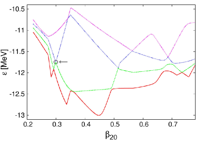
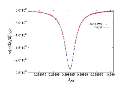
Figure 15: Left panel: s.p. energies in the Woods-Saxon potential along the chosen nonaxial path (parametrized by $\beta_{20}$, Fig. 10); a sharp pseudocrossing is marked by a circle. Right panel: adiabatic coupling between the two levels in the vicinity of crossing and its fit by a model curve (43).

We kept the adiabatic basis. In order to integrate Eq. (12) we used a changing step in $\beta_{20}$ for calculating input data, i.e. energies and adiabatic couplings along the path. The step $\Delta\beta_{20}$ was diminished when a change in any of the couplings was above 10% of its preceding value. It was necessary to impose the minimal step value, $\Delta\beta_{20}=10^{-7}$ (with $\beta_{20}$ as the parameter of the path). Such a probing was dense enough for a nearly exact integration for most of the peaks. However there were a few narrow and high peaks which were still not well rendered. In those cases, the shape of such peak was modelled by the formula (43) (with parameters $\alpha$ and $q_{0}$) using the least squares fit to the calculated points. Next, for each such modelled crossing, a $2\times 2$ transition matrix $\mathbf{G}(\tau_{fin},\tau_{ini})$ for the two crossing levels was integrated [defined by the Eq. (69)], where $\tau_{ini},\tau_{fin}$ means the beginning and end of the peak. The integration of a model peak is simple due to its analytic formula which makes many Woods-Saxon calculations unnecessary. Then the propagation matrix $\mathbf{\widetilde{G}}(\tau_{fin},\tau_{ini})$ for all ${\cal N}$ levels is calculated as follows: propagation of the ${\cal N}-2$ not crossing levels is done in a standard way while for two crossing levels one substitutes the matrix $\mathbf{G}$ calculated for the fitted model. Denoting the index of the lower crossing level $i$, one can schematically write the matrix $\mathbf{\widetilde{G}}$:

$$\bordermatrix{&1&2&\ldots&i&i+1&\ldots&{\cal N}\cr 1&\widetilde{G}_{11}&\widetilde{G}_{12}&\ldots&0&0&\ldots&\widetilde{G}_{1{\cal N}}\cr 2&\widetilde{G}_{21}&\widetilde{G}_{22}&\ldots&0&\ 0&\ldots&\widetilde{G}_{2{\cal N}}\cr\vdots&\vdots&\vdots&\ddots&\vdots&\vdots&\ddots&\vdots\cr i&0&0&\ldots&G_{i\ i}&G_{i\ i+1}&\ldots&0\cr i+1&0&0&\ldots&G_{i+1\ i}&G_{i+1\ i+1}&\ldots&0\cr\vdots&\vdots&\vdots&\ddots&\vdots&\vdots&\ddots&\vdots\cr{\cal N}&\widetilde{G}_{{\cal N}1}&\widetilde{G}_{{\cal N}2}&\ldots&0&0&\ldots&\widetilde{G}_{{\cal N}{\cal N}}\cr}$$ (72)

Thus, we neglect the cross terms, setting: $\mathbf{\widetilde{G}}_{\alpha l}=\mathbf{\widetilde{G}}_{l\alpha}=0$, where $\alpha\neq i,\,i+1$ and $l=i,\,i+1$. It means we treat the crossing of two levels as isolated: the evolution of $c_{i},c_{i+1}$ is dominated by the coupling between them, $\langle\phi_{i}|\partial_{q}\phi_{i+1}\rangle$, while the effect of other states $c_{\alpha\neq i,i+1}$ on crossing levels and the effect of the pair on those other states can be neglected in the vicinity of crossing.

This procedure was tested in few cases in which the vicinity of the crossing could be probed dense enough for the solution without any fit to be exact. Then the solutions for smaller density of calculated points but with the modelled adiabatic coupling in the vicinity of crossing was compared to the exact one. It turned out that for the desired accuracy the model for the coupling should include independent parameters for the height and half-width:

$$\left\langle\phi_{1}\bigg{|}\frac{d\phi_{2}}{dq}\right\rangle=\frac{1}{2}\frac{\alpha}{(q-q_{0})^{2}+\sigma^{2}}.$$ (73)

With this model, the calculated actions differed less than 1% from the reference results, except for very small actions, for which the difference was of no consequence anyway.

References

- (1) D. R. Inglis, Phys. Rev. 96, 1059 (1954), Phys. Rev. 103, 1786 (1956)
- (2) M. Brack, J. Damgøard, A. S. Jensen, H. C. Pauli, V. M. Strutinsky, and C. Y. Wong, Rev. Mod. Phys. 44, 320 (1972)
- (3) M. Baranger and M. Veneroni, Ann, Phys. (NY) 114, 123 (1978)
- (4) M. J. Giannoni and P. Quentin, Phys. Rev. C 21, 2060 (1980)
- (5) J. Dobaczewski and J. Skalski, Nucl. Phys. A 369, 123 (1981)
- (6) Z. Łojewski, A. Baran, Z. Phys. A 322, 695 (1985)
- (7) M. Mirea, Phys. Rev. C 100, 014607 (2019)
- (8) The formula (I) presents also a problem of low-energy collective excitations, in particular, rotations: in odd- nuclei, there may be rotational states with the same and similar energy as the g.s., built on other one-quasiparticle configuration. While transitions to such states are not forbidden by any strict conservation laws, they are not accounted for in the derivation of (I).
- (9) F. P. Hessberger, Eur. Phys. J. A 53, 75 (2017)
- (10) S. Coleman, Phys. Rev. D 15, 2929 (1977), C. G. Callan, and S. Coleman, Phys. Rev. D 16, 1762 (1977)
- (11) S. Levit, J.W. Negele and Z. Paltiel, Phys. Rev. C 22, 1979 (1980)
- (12) J. W. Negele, Rev. Mod. Phys. 54, 913 (1982)
- (13) G. Puddu, and J. W. Negele, Phys. Rev. C 35, 1007 (1987)
- (14) J.W. Negele, Nucl. Phys. A 502, 371 (1989)
- (15) E. M. Chudnovsky and J. Tejada, ”Macroscopic Quantum Tunneling of the Magnetic Moment” (Cambridge University Press,1998)
- (16) G. M. Mil’nikov, H. Nakamura J. Chem. Phys. 115, 6881 (2001)
- (17) A. Andreassen, D. Farhi, W. Frost, and M. D. Schwartz, Phys. Rev. D 95, 085011 (2017)
- (18) P. Ring, P. Schuck ”The Nuclear Many Body Problem”, Springer-Verlag 1980
- (19) J. Skalski, in Proc. Int. Workshop on ”New Developments in Nuclear Self-Consistent Mean-Field Theories (MF05)”, Yukawa Institute for Theoretical Physics reports series YITP-W-05-01 (Soryushi-ron Kenkyu) (2005), p. B62; on the web: http://wwwnucl.ph.tsukuba.ac.jp/MF05/proceedings.html.
- (20) J. Skalski, Phys. Rev. C 77, 064610 (2008)
- (21) J. Skalski, Int. J. Mod. Phys. E 18, 798 (2009)
- (22) D. J. Thouless, and J. G. Valatin, Nucl. Phys. 31, 211 (1962)
- (23) One can show this e.g. by using the expression for action in terms of the operator of (17), given by the formula (44) in JS , and expanding instantons onto eigenvectors of .
- (24) A. Bulgac, Phys Rev. C 41, 2333 (1990)
- (25) Y. M. Engel, D. M. Brink, K. Goeke, S. J. Krieger, and D. Vautherin, Nucl. Phys. A 249, 215 (1975)
- (26) Meng-Hock Koh, L. Bonneau, P. Quentin, T. V. Nhan Hao, and Husin Wagiran, Phys. Rev. C 95, 014315 (2017)
- (27) S. E. Koonin and J. R. Nix, Phys. Rev. C 13, 209 (1976)
- (28) L. Landau, Physikalische Zeitschrift der Sowjetunion 2, 46 (1932)
- (29) C. Zener, Proceedings of the Royal Society of London A 137, 696 (1932)
- (30) E. C. G. Stückelberg, Helv. Phys. Acta 5, 370 (1932)
- (31) W. Brodziński, P. Jachimowicz, M. Kowal, J. Skalski, Acta Phys. Pol. B Vol. 49, 621 (2018)
- (32) S. Ćwiok, J. Dudek, W. Nazarewicz, J. Skalski and T. Werner, Comput. Phys. Commun. 46, 379 (1987)
- (33) H. J. Krappe, J. R. Nix and A. J. Sierk, Phys. Rev. C 20, 992 (1979)
- (34) I. Muntian, Z. Patyk, and A. Sobiczewski, Acta Phys. Pol. B 32, 691 (2001)
- (35) P. Jachimowicz, M. Kowal, J.Skalski, Phys. Rev. C. 89, 024304 (2014)
- (36) M. Kowal, P. Jachimowicz, and A. Sobiczewski, Phys. Rev. C 82, 014303 (2010)
- (37) P. Jachimowicz, M. Kowal, and J. Skalski, Phys. Rev. C 85, 034305 (2012)
- (38) P. Jachimowicz, M. Kowal, and J. Skalski, Phys. Rev. C 95, 014303 (2017)
- (39) P. Jachimowicz, M. Kowal, and J. Skalski, Phys. Rev. C 101, 014311 (2020)
- (40) D.L. Hill, J.A Wheeler, Phys. Rev. 89, 1102 (1953)
- (41) We omit here a small difference in W-S potentials for nuclei and .
- (42) P. Moller, private communication
- (43) Z. Łojewski, A. Baran, Z. Phys. A 329, 161 (1987)
- (44) R. Smolańczuk, J. Skalski and A. Sobiczewski, Phys. Rev. C 52, 1871 (1995)
- (45) R. Smolanczuk. Phys. Rev. C 56, 812 (1997)
- (46) S. E. Koonin, R. L. Hatch and J. Randrup, Nucl. Phys A 238, 87 (1977)
- (47) D. Rouvel, PhD Thesis, University of Strasbourg, (2014); D. Rouvel, J. Dudek, Phys. Rev. C 99, 041303(R) (2019)
- (48) M. V. Berry, Proc. R. Soc. Lond. A 392, 45 (1984)
- (49) K. K. Kan, Phys. Rev 24, 279 (1981)
- (50) S.E. Koonin, D.J. Dean, and K. Langanke, Phys. Rep. 278, 1-77 (1997)
- (51) C. A. Mead and D. G. Truhlar, J. Chem. Phys. 77, 6090 (1982)
- (52) M. Baer, Chem. Phys. Lett. 35, 112 (1975)
- (53) J. Q. Sun and C. D. Lin, J. Phys. B 25, 1363 (1991)
- (54) T.Pacher, L.S. Cederbaum, H.Köppel, J. Chem. Phys. 89, 7367 (1988)