Accurate Characterization of Non-Uniformly Sampled Time Series using Stochastic Differential Equations

Abstract

Non-uniform sampling arises when an experimenter does not have full control over the sampling characteristics of the process under investigation. Moreover, it is introduced intentionally in algorithms such as Bayesian optimization and compressive sensing. We argue that Stochastic Differential Equations (SDEs) are especially well-suited for characterizing second order moments of such time series. We introduce new initial estimates for the numerical optimization of the likelihood, based on incremental estimation and initialization from autoregressive models. Furthermore, we introduce model truncation as a purely data-driven method to reduce the order of the estimated model based on the SDE likelihood. We show the increased accuracy achieved with the new estimator in simulation experiments, covering all challenging circumstances that may be encountered in characterizing a non-uniformly sampled time series. Finally, we apply the new estimator to experimental rainfall variability data.

I Introduction

Non-uniformly sampled time series are found in a wide range of applications. They typically occur when the experimenter has limited control over signal sampling. Sampling times may be determined by a natural process, for example in turbulent flow characterization using laser-Doppler anemometry [1], analysis of climate time series [2] and astronomy [3]. Alternatively, non-uniform sampling can occur because of an irregular human sampling, e.g. in power systems sensor data [4], oil production surveillance [5] and vital signs measurements in medical applications [6, 7]. Finally, non-uniform sampling is a key attribute of certain algorithms, including Bayesian optimization [8] and compressive sensing [9].

It has been shown theoretically that alias-free spectral estimates can be obtained using non-uniform sampling[10]. As most theoretical results, this result is asymptotic, i.e., it holds in the limit where the number of observations $N$ tends to infinity. The result can easily be understood intuitively, as follows: As a signal is sampled at random times for a long enough time, any desired number of observations is a available at an arbitrarily low sampling interval. Hence, the spectrum can be estimated alias-free up to an arbitrary high frequency. Following the same intuition, it is clear that this asymptotic result breaks down for finite $N$, because the shortest time interval will be finite in that case.

The objective of this work is to accurately characterize the second order moments of a non-uniformly sampled stationary stochastic process, which can be expressed in terms of the power spectral density in the frequency domain. Given the close correspondence between the error in the log power spectrum and the Kullback-Leibler discrepancy [11], we will use “spectral estimation” as a shorthand for the aforementioned objective. In the time domain, the second order moments are expressed using the covariance function, or, equivalently, the kernel of a Gaussian processes [12].

Existing approaches include non-parametric methods, such as the Lomb-Scargle spectral estimate [13], and the slotting technique for estimation of the covariance function [14]. Parametric techniques include discrete-time autoregressive models [15] and stochastic differential equations with random initial estimates [16]. While parametric techniques show the most promising results, previous work also report inaccurate spectral spectral estimates at higher frequencies for higher-order models, and sensitivity to initial conditions of the maximum likelihood (ML) fitting procedure [17, 18], which limit the practical use of these algorithms.

Our main contribution is to propose a new algorithm for spectral estimation using Stochastic Differential Equations (SDEs) based on incremental parameter estimation and data-driven model truncation, that has been validated in simulation experiments. We explain how model truncation in SDEs results greater accuracy than discrete-time models through analyzing the SDE(1) case. For the problem of spectral estimation from non-uniformly sampled time series, asymptotic theory provides a poor description of actual behavior. Hence, simulation experiments are indispensable to establish the accuracy of an estimator, and are therefore a key component of this paper.

In section II, we motivate the usage of SDEs for spectral estimation and provide a number of basic definitions and results. Section III describes the new SDE parameter estimation procedure. Section IV contains the design of the simulation experiments, which is used in section V to quantify the error reduction achieved through model truncation, and in section VI for the overall evaluation of the proposed estimator. Finally, we apply the estimator to experimental rainfall variability data in section VII.

II Stochastic Differential Equations: Motivation and definitions

We use stochastic differential equations (SDEs) to estimate the power spectral density of a time series. We motivate this choice over available alternatives as follows:

• By using a parametric model we can formulate of a maximum likelihood (ML) estimator. Unlike many non-parametric estimators, ML estimators have desirable theoretical properties such as asymptotic efficiency. Parametric spectral estimators have been most successful at achieving the benefit of high-frequency spectra in finite samples [15], whereas non-parametric methods such as the Lomb-Scargle estimator [13] have very high variance, which mostly limits their use to finding a single peak in the spectrum under high signal-to-noise conditions. Similarly, in the time domain, correlation estimated with the non-parametric slotting technique violate the positive-definiteness property that is required for a valid autocorrelation function [14]. Parametric models can achieve the same flexibility as non-parametric estimates by increasing the model order.

• The SDE model is a continuous time model, which can operate directly on non-uniform samples without the need to introduce a regular grid as is required for discrete-time estimates. Moreover, estimated discrete time time series models may have poles that do not have a continuous-time counterpart [19].

The stochastic differential equation of order $p$ for the process $y$ as a function of time $t$ is given by:

$$\frac{d^{p}y}{dt^{p}}+\sum_{i=1}^{p}a_{i}\frac{d^{i-1}y}{dt}=\epsilon$$ (1)

where $a_{i}$ are the SDE coefficients, collectively denoted $\mathbf{a}$, and $\epsilon$ is continuous Gaussian white noise with standard deviation $\sigma_{\epsilon}$.

The SDE model can be rewritten as an equivalent state-space model:

$$\frac{d\mathbb{\mathbf{z}}}{dt} =\mathbf{A}\mathbf{z}+\mathbf{\epsilon}$$ (2)

$$y =C\text{$\mathbf{z}$}$$

where the state $\mathbf{z}$ and $\mathbb{\epsilon}$ are $p$-dimensional time series and $C\mathbf{z}=z_{1}$. The matrix $\mathbf{A}$ and the covariance matrix $\mathbf{Q}$ of $\mathbb{\epsilon}$ can be computed from $\left\{\mathbf{a},\sigma_{\epsilon}\right\}$, see [20].

The SDE process has a power spectral density given by [21]:

$$h_{y}\left(f\right)=\mathbf{C}\left(\mathbf{A}-i2\pi f\mathbf{I}\right)^{-1}\mathbf{Q}\left(\mathbf{A}+i2\pi f\mathbf{I}\right)^{-T}\mathbf{C}^{T}$$

and the covariance function at lag $\tau>0$ of:

$$R\left(\tau\right)=\mathbf{\mathbf{P}}_{s}\exp\left(\mathbf{A}t\right)^{T}$$ (3)

where $\mathbf{\mathbf{P}}_{s}$ is the stationary covariance matrix.

The state space equation may be diagonalized to represent the SDE as:

$$\frac{d\mathbb{\mathbf{z}}^{\prime}}{dt} =\Lambda\mathbb{\mathbf{z}}^{\prime}+\mathbf{\epsilon^{\prime}}$$

$$y= C^{\prime}\text{$\mathbf{z}$}^{\prime}$$

where the eigenvalues are equal to the the roots $r_{i}$ (collectively denoted $\mathbf{r}$) of the characteristic equation of (1) for $\epsilon=0$, and $C^{\prime}\text{$\mathbf{z}$}^{\prime}=\sum z^{\prime}_{i}$. We refer to this parameterization as the roots parameterization, while we refer to the $\left\{\mathbf{a},\sigma_{\epsilon}\right\}$ parameterization as the coefficients parameterization.

The key advantage of the roots parameterization is that stationarity can be expressed as the requirement that the real part of the roots is negative : $\textrm{Re}\left(r_{i}\right)<0$. Furthermore, the computational complexity of the likelihood computation is more efficient for large model order $p$.

Despite the advantages, many researchers use the coefficient representation. This may be motivated by the reduced computational complexity for lower-order models. In addition, SDEs can be used to parameterize a kernel as part of a larger machine learning model, e.g. in deep learning models [22] or for posterior sampling using a probabilistic program [23]. Currently many major automatic differentiation packages such as PyTorch [24] and the Stan autodiff library [25] do not support complex-valued parameters, therefore necessitating the use of the coefficient representation. Therefore, we consider both representations in this work.

III Maximum likelihood estimation

III-A Likelihood computation

The exact log likelihood $L$ is computed recursively using the Kalman filtering equations. Process stationarity is exploited for the first observation, i.e., it has the stationary covariance matrix $\mathbf{P}_{s}$. Given a value for the SDE parameters $\mathbf{a}$ or $\mathbf{r}$, the analytical expression for the Maximum Likelihood standard deviation $\sigma_{\epsilon}$ is used [20]. For unstable models, or errors due to the finite machine precision, a log likelihood of $L=-\infty$ is produced.

The computation largely follows cited algorithms, with the following improvements to increase computational efficiency:

1. For the coefficient representation, we follow [21] for the measurement and likelihood steps. The prediction step computes the conditional mean $\mathbf{\mu}_{n|n-1}$ and covariance matrix $\mathbf{P}_{n|n-1}$ of the state $\mathbf{z}_{n}$:

   $$\mathbf{\mu}_{n|n-1} = \mathbf{F}\mathbf{\mu}_{n-1}$$

   $$\mathbf{P}_{n|n-1} = \mathbf{F}\mathbf{P}_{n-1}\mathbf{F}^{T}+\int_{\tau=0}^{\Delta t}\exp(\mathbf{A}\tau)\mathbf{Q}\exp(\mathbf{A}\tau)^{T}d\tau$$

where $\mathbf{F}=\exp\left(\mathbf{A}t\right)$. To compute the integral, instead of using the Matrix Fraction Decomposition proposed in [21], we eliminate the covariance matrix $\mathbf{Q}$ to yield:

$$\mathbf{P}_{n|n-1} =\mathbf{P}_{s}-\mathbf{F}(\mathbf{P}_{s}-\mathbf{P}_{n-1})\mathbf{F}^{T}$$

1. For the root representation, we use the algorithm in [20], with the following alternative computation for the stationary covariance matrix $\mathbf{P}^{\prime}_{s}$:

   $$\left[\mathbf{P}^{\prime}_{s}\right]_{ij}=-\frac{\left[\mathbf{Q}^{\prime}_{s}\right]_{ij}}{\left(r_{i}+\bar{r_{j}}\right)},$$

   which is a corollary of eq. 30 in [20] for $t_{k}-t_{k-1}\rightarrow\infty$.

Given the extensive literature on Kalman filtering, these improvements may have been previously reported in the literature. We still report them here to accurately represent to algorithms used in this work.

III-B Optimization

Optimization of the likelihood is performed using the Limited-Memory BFGS algorithm [26], with derivatives obtained through automatic differentiation. For the coefficient representation, a necessary condition for stability is that all coefficients $a_{i}$ are positive; it is also sufficient for $p\leq 2$ [27]. To improve optimization results, parameter values are constrained to a configurable interval: $a_{i}\in\left\langle a_{l},a_{h}\right\rangle$. Wide limits should be set to allow for a wide range of models. As an indication, $a_{l}$ is related to the duration $D$ of the time series $a_{l}\lesssim 1/D$, and $a_{h}$ is related to the shortest sampling interval $\Delta t_{m}$, $a_{h}\gtrsim 1/\Delta t_{m}$. In the presented simulation results, we use $a_{i}\in\left\langle 10^{-3},10^{3}\right\rangle$. In the roots representation, the real and imaginary part of the roots are similarly constrained.

III-C Initialization

Accurate initialization of the optimization is key to achieving high-quality estimates. The sensitivity of SDE parameter estimation to initial conditions has been acknowledged in the literature [17], in particular for higher-order models [18].

The first element in the algorithm is incremental estimation: The estimate for the SDE($p$) model is initiated from a lower order SDE($p^{\prime}$) model ($p^{\prime}<p$). The motivation for incremental estimation is the observation that per parameter, lower order models often have the largest contribution to the model fit. The lower order models are expanded by adding a single random real root (for $p^{\prime}=p-1$) or a conjugate pair of random complex roots (for $p^{\prime}=p-2$) to the lower order model. An alternative for a this root initialization would be to use a large initial value, as this corresponds to a model that is most similar to the lower-order model. However, this extreme initialization does not result in successful convergence to a finite value during the numerical optimization.

The second element is initiation from autoregressive (AR) models estimated from resampled data using the Burg estimator [28]. Resampling is performed using nearest neighbor interpolation and linear interpolation. Intentionally, basic interpolation methods are used here, because more advanced interpolation methods tend to produce artificially smooth signals, or, in the frequency domain, a power spectrum with a very large dynamic range. This results in less accurate models, since the estimators attempts to fit the artificially introduced low power spectral density at high frequencies, at the expense of modeling the actual process dynamics [11]. AR roots that do not have a corresponding continuous-time root [19] are replaced by randomly generated roots.

The usage of autoregressive models is similar to the methodology proposed in [29] for reducing the variance in spectral estimates based on AR models. However, our work is distinct in the following aspects: (i) we do not need to introduce an arbitrary criterion to remove roots in the upper half of the spectrum, which could eliminate true spectral peaks, and (ii) we only use the AR model as an initial estimate, allowing further optimization of the likelihood during numerical optimization.

These main components are supplemented with purely random initialization [16, 30] and a truncation phase that occurs after incremental estimation, where successively lower model orders are initiated from the most significant roots of higher order models.

III-D Implementation

The estimator is implemented in Julia 1.4, using Optim.jl [31] for L-BFGS optimization. Gradients are computed with automatic differentiation using Zygote.jl [32]. Julia was used because it combines an expressive syntax with high execution speed. Zygote is a package for automatic differentiation that supports all functions used in the likelihood computation, notably including the matrix exponential [33], and supports complex-valued parameters.

IV Design of experiments

IV-A Test processes

The experiment is designed to cover the following process characteristics that are challenging for parameter estimation from non-uniformly sampled data:

1. Overfit: When the order of the estimated model matches the order that of the generating process, accurate models can be estimated [15]. However, the additional flexibility of a higher order parameters can lead to large errors, more so than the small statistical error that is observed in parameter estimation from regularly sampled data.

2. High dynamic range: Estimation of the spectral density at frequencies where the true density is low is challenging for many estimators, due to a phenomenon similar to spectral leakage [34].

3. Spectral details beyond average sampling rate: While asymptotic theory predicts alias-free estimates, capturing spectral details at higher frequency remains challenging in practice, because limited information high-frequency information is available in finite samples.

4. Model misspecification: Any estimation procedure should continue to work well when the actual process cannot be described exactly using the estimated model structure.

To cover these characteristics, we use the following test processes:

• Case A: SDE(1) process with parameter $a_{1}=-1/200$. Covariance function: $R\left(\tau\right)=\exp\left(a_{1}\tau\right)$. Addresses characteristics #1 and #2.

• Case B: Squared exponential covariance with scaling parameter $l=0.3$ with added random noise with $\sigma_{w}=0.01$. Covariance: $R\left(\tau\right)=\exp\left(-\tau^{2}/l^{2}\right)+\sigma_{w}^{2}\delta\left(\tau\right)$. Addresses #2, #4.

• Case C: SDE(4) process with roots $\left\{-0.10\pm 2\pi\cdot 0.25i,-0.5\pm 2\pi\cdot 1.5im\right\}$ . Addresses #1, #3.

• White noise: A temporally uncorrelated process. Covariance function $R\left(\tau\right)=\delta\left(\tau\right)$, where $\delta\left(0\right)=1$, and $0$ elsewhere. Addresses: #1.

Non-uniform sampling times are generated by drawing $N=200$ time intervals from a Poisson distribution with average sampling interval $T_{av}=1$. Samples $\mathbf{y}$ from a process $P$ are drawn for the resulting sampling times $\mathbf{t}$. In this way, $S=50$ time series $\left\{\mathbf{t},\mathbf{y}\right\}$ are generated for each process. For the simulated data, SDE(8) models are estimated. The results of the simulation experiments are discussed in the subsequent sections.

IV-B Kullback-Leibler Discrepancy

Our objective is to accurately characterize the second-order moments of a random process, which we quantify using the The Kullback-Leibler Discrepancy (KLD). The KLD has a number of desirable properties. First, it has units that are statistically meaningful. For an unbiased estimate of a $d$-dimensional parameter $\theta$ that achieves the Cramér-Rao lower bound, the expected value of the KLD is asymptotically equal to $d/2$: $\textrm{E}\left[D\left(\hat{\mathbf{\theta}}\mathbf{\|\mathbf{\theta}}\right)\right]=d/2$. For the SDE($p$) model we estimate $p+1$ parameters (adding 1 to $p$ for estimation of $\sigma_{\epsilon}$), yielding:

$$\textrm{E}\left[D\left(\hat{\mathbf{\theta}}\mathbf{\|\mathbf{\theta}}\right)\right]=\left(p+1\right)/2.$$ (4)

A second desirable property is that, for time series models, the KLD is asymptotically equivalent to the spectral distortion (Root Mean Square Error (RMSE) of the log power spectrum) and the normalized one-step ahead prediction error. See e.g. [11] for further background on these properties.

The KLD for a zero-mean multivariate Gaussian model for a random vector $\mathbf{y}$ with covariance matrix $\hat{\Sigma}$ with respect to the true zero-mean distribution with covariance matrix $\Sigma$ is given by:

$$D\left(\Sigma\|\hat{\Sigma}\right)=\frac{1}{2}\left(\mathrm{tr}\left(\hat{\Sigma}^{-1}\Sigma-I\right)-\log\text{$\left(\left|\Sigma\right|/\hat{\left|\Sigma\right|}\right)$}\right)$$ (5)

For SDE models, $\mathbf{y}$ is the vector of time series observations at times $\mathbf{t}$. The covariance matrix is computed using the covariance function from eq. 3. The choice of time steps $\mathbf{t}$ determines the time scale at which we evaluate the process.

One value for $\mathbf{t}$ is the original time points of the dataset to which the estimated model is fitted. The resulting KLD is referred to as $D_{o}$. A second value for $\mathbf{t}$ is a regularly spaced grid at interval $T$, referred to as $D_{T}.$ The value of $T$ corresponds to the time scale of interest at which we evaluate the second order moments. In the frequency domain, the corresponds to evaluating the power spectrum for frequencies up to the corresponding Nyquist frequency, $f=1/2T$.

The KLD does not suffer from some problems associated with some alternative ways to evaluate estimates:

• Look for the “correct” or “actual” order: Practical processes typically cannot be described exactly by a finite order model. Even if such a finite order model would exist, estimating a model of this order may not result in the most accurate estimate due to estimation errors.

• RMSE of estimated SDE coefficients or autocovariance: A small change coefficients or autocovariance values can result in a completely different process, e.g. changing from stable to unstable (coefficients), or positive-definite (valid) to not positive-definite (invalid) for autocovariances [14].

The base implementation of the KLD is computationally expensive. If required, a more efficient asymptotic expression can be derived specifically for SDE models. We do not elaborate on this here, because this computation is only used to evaluate model performance in simulations. It not part of the estimation algorithm, and so it will not increase computation times for the end user. Furthermore, the generic expression allows evaluation of non-SDE processes such as the squared exponential covariance function.

V Data-driven model truncation

In this section we describe the phenomenon of parameter divergence in SDE parameter estimation, and how it can be exploited to reduce the cost of model overfit.

V-A Model truncation for the SDE(1) model

As parameters are optimized to maximize the likelihood, parameter estimates can diverge to infinity, resulting in numerical problems in the likelihood computation [20]. Also, it has been reported that not all AR models have a continuous-time counterpart [19]. In this section, we show how these phenomena are closely related through a theoretical analysis of the the SDE(1) model. Furthermore, we show how this phenomenon ultimately results in more accurate estimates.

The SDE(1) model is an important model for many applications. It is also known in the literature as the Ornstein-Uhlenbeck process and is a special case of the Matérn kernel [12]. For data regularly sampled at interval $T$, the maximum likelihood estimate of the SDE(1) parameter $\hat{a}$ can be computed analytically [21]:

$$\hat{a}=\frac{1}{T}\log\left[\hat{\alpha}\right]$$

where $\hat{\alpha}$ is the estimated AR(1) parameter. For a white noise process, the estimated AR(1) parameter is distributed symmetrically around $\hat{\alpha}=0$ with standard deviation $1/\sqrt{N}$, where $N$ is the number of observations [35]. Hence, $\hat{\alpha}$ is negative for 50% of signals. In this case, the AR(1) process has no continuous-time counterpart.

It can be shown that, under these conditions, the likelihood monotonically increases for $a\rightarrow\infty$. In this limit, the SDE(1) model is equivalent to the white noise model. In practice, the true model order is unknown, and so it is critical that an estimator returns an accurate estimate under these circumstances. This is achieved using data-driven model truncation. With model trunction, the estimation algorithm for an SDE($p$) model can return a lower SDE($p^{\prime}$) model if the likelihood indicates that the lower order model fits better to the data. For the SDE(1) case, this amounts in returning an SDE(0) or white noise model when $\hat{\alpha}<0$. We discuss model truncation for higher order models in the next section.

V-B Model truncation for higher order models

As described in section III-C, SDE($p$) models are estimated incrementally. If parameter divergence occurs, the model returned by the optimization procedure has large but finite values because of the limits introduced on parameter values. In this case, the lower order model will have a larger likelihood, and is consequently the final maximum likelihood estimate. While this phenomena can be easily analyzed for the SDE(1) model estimated from white noise, this is an important phenomena more generally, as it occurs whenever the order of the estimated model is greater than the true model order. Since the true model order is unknown for experimental data, it is desirable to estimate a high order model, so that a wide range of processes can be represented. Model truncation reduces the cost of overfit, i.e., the statistical estimation error induced by estimation SDE($p$) models where $p$ exceeds the true model order.

V-C KLD reduction achieved in white noise

Adding to the theoretical analysis of the SDE(1) case, we quantify the improvement that is achieved with data-driven model truncation in a simulation experiment where SDE models are estimated from a non-uniformly sampled white noise process. The Kullback-Leibler discrepancy $D_{o}$ as a function of model order is given in figure 1, along with the theoretical expected value for the KLD $D_{o}$ from eq 4. We use $D_{o}$ here, because it uses the same time vector $\mathbf{t}$ as the likelihood. Therefore, we can use the theoretical expectation (4).

As expected, we observe a significant reduction in the error for higher order models due to model truncation. Because the theoretical expression is accurate for the discrete-time AR models, these results also quantify the error reduction compared to AR models.

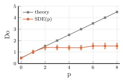
Figure 1: Kullback-Leibler Discrepancy (KLD) $D_{o}$ as a function of SDE model order $p$ estimated from non-uniformly sampled white noise. Because of data-driven model truncation, the KLD observed in simulation experiments for estimated SDE($p$) models is below the theoretical prediction for the KLD.

VI Estimator performance

In this section, we discuss estimator performance across the test cases A, B and C introduced in section IV. Figure 2 shows the average KLD at interval $T=0.2$, $D_{0.2}$, as well as sample spectral estimates compared to the true spectrum up to the Nyquist frequency corresponding to the KLD interval: $f=1/2T=2.5$. Note that we use a KLD at a time interval $T$ that is considerably shorter than the average sampling interval $T_{av}=1$. This allows us to quantify the estimator capability to characterize the process at short time scales, or, in the frequency domain, up to frequencies beyond the Nyquist rate corresponding the the average sampling time: $f_{N,Tav}=0.5$. Estimates are shown for the SDE(8) ML estimate obtained using the roots parameterization ($\mathbf{r}$), referred to as the “MLE root” estimate.

We conclude that this estimator reliably estimates the power spectrum for the test processes, which cover all of the challenging conditions listed in section IV-A. Accurate estimates can be obtained well above $f_{N,Tav}$. The squared exponential case is the most challenging case, because of the joint occurrence of model misfit and a high dynamic range. For this case, estimates are less accurate across the entire frequency range because of statistical estimation errors.

We specifically draw attention to the absence of large erroneous peaks in the spectral estimates, as they have been reported previously in the literature, including a study of the autoregressive (AR) ML estimator for similar test cases [36]. The absence of these peaks in the SDE estimate is a consequence of the data-driven model truncation introduced in section V, and results in substantially more accurate spectral estimates. Compared to [36], the model accuracy is much improved for cases A and B. Only in case C, the AR ML estimate in [36] is more accurate. However, for this case, a model of the true order (AR(4)) was estimated instead of an AR(8) model, explaining the absence of erroneous peaks. In general, we cannot assume knowledge of the true model order of the generating process for a given experimental dataset.

Given the remarkable success in suppressing erroneous peaks compared to previous work, the relevance of case C is to show the capability of the estimator to accurately estimate true spectral peaks at a high frequency. Here, our work has a key advantage over the algorithm proposed in [29], in which all high frequency AR roots are eliminated.

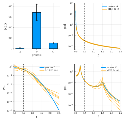
Figure 2: Accuracy of SDE(8) models estimated from simulated data, sampled non-uniformly at an average sampling time of $T_{av}=1$ ($S=50$ simulation runs for each case A, B and C). Left top: Kullback-Leibler Discrepancy at time interval $T=0.2$ ($D_{0.2}$), averaged over all simulation runs. Remaining graphs: Representative sample spectral estimates computed from the SDE(8) estimates, compared to the true power spectrum up a frequency of $1/2T=2.5$. Accurate estimates are achieved across the entire frequency range, going well beyond the Nyquist frequency for the average sampling interval $f_{N,Tav}=0.5$, which is indicated by the black dashed line.

Figure 3 compares the accuracy of the “MLE root” estimator to two alternative estimators: the coefficient parameterization “MLE coef” and random root initiation (“random init root”). While all estimators perform well for the basic SDE(1) case A, the “MLE coef” and “random init root” estimators have reduced quality for the more complex cases B and C, that require accurate higher order SDE estimates for accurate results.

For the “MLE coef” estimator, the reduced quality can be explained from the fact that the likelihood computation is less numerically stable. Also, for models of order $p>3$, the search space of positive coefficients also contains non-stationary models. The performance degradation is greatest for the “random init root” estimator, with an increase of a factor of 4 case C. While random initiation converges to a good solution for many simulations, it occasionally fails to find a good optimum resulting in a very large error. This performance degradation is expected to increase further with increasing model order.

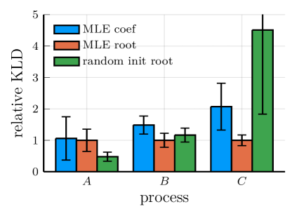
Figure 3: Comparison of the estimation accuracy of 3 alternative SDE parameter estimators. The reported values are the Kullback-Leibler Discrepancy $D_{0.2}$ relative to the “MLE root” estimate.

VII Analysis of monsoon rainfall variability

Long-term variability in monsoon rainfall is studied using radiometric-dated, speleothem oxygen isotope $\delta^{18}O$ records [37]. The data is intrinsically irregularly sampled, because it is formed by natural deposition rather than experimenter controlled sampling. For the same reason, irregular sampling occurs for many other long-term climate records as well, e.g. ice core data [38].

The average sampling rate of speleothem data depends on the measurement location. The current dataset is suitable for algorithm benchmarking because it has a higher average sampling rate than datasets collected from other locations. This allows us to study algorithm performance for different sampling rates, by subsampling the original data, and comparing the results to estimates obtained from the full dataset. Also, the dataset is publicly available as supplementary material to [37] for reproducibility of results. The oxygen isotope data consists of $N=1848$ irregularly sampled observations of $\delta^{18}O$ anomalies over a time span of $2147$ years, resulting in average sampling interval of $T_{0}=1.16$ years.

We estimate SDE(8) models from detrended $\delta^{18}O$ data. A reference estimate is obtained using the complete dataset. To emulate a lower sampling rate, we then estimate models from $5$ random subsets of the original data, at an average sampling interval of $T_{av}=5$ years. The resulting estimated spectra and model fit are given in figure 4. The reference SDE(8) model is truncated to an SDE(1) model. Models estimated from the subsampled data similarly exploit model truncation to achieve accurate spectral estimates, avoiding erroneous peaks in the estimate, despite a much lower sampling frequency compared to the full dataset. The maximum likelihood is achieved at either order $p=1$ (4 out of 5 subsets) or $p=5$ (1/5) (see figure 4, bottom).

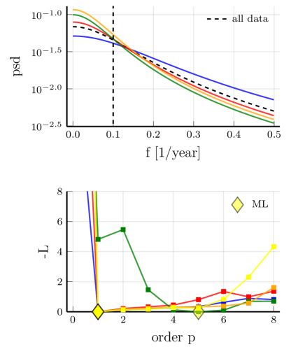
Figure 4: Top: Power spectra estimated from detrended speleothem oxygen isotope $\delta^{18}O$ data using SDE(8) estimates. Estimates are based either on all data (black dashed line), or on subsets of data (colored lines) that are randomly subsampled at an average sampling interval $T=5$ years. While based on a much smaller dataset, the estimates from subsampled data remain accurate. Bottom: Model fit (negative log likelihood $L$) as a function of model order for the models estimated from subsampled data, with colors corresponding to the same subsets as in the top spectrum plots. The yellow diamond indicates the order of the ML estimate after data-driven model truncation.

VIII Concluding remarks

The proposed SDE-based method for spectral estimation from non-uniformly sampled data provides a more accurate estimate than existing methods. This is achieved using more accurate initialization combined with data-driven model truncation. We have shown the performance of this estimator in simulation experiments, and by application of the algorithm to experimental rainfall variability data.

Further advances can be achieved through model regularization. One way to achieve regularization is by means of order selection. Novel order selection criteria can be developed based on the reported behavior of SDE estimators in figure 1. This behavior deviates significantly from the theoretical behavior on which criteria such as the Akaike Information Criterion are based.

Alternatively, regularization can be achieved by introducing informative priors in a Bayesian approach. This has shown promise in discrete time estimation, albeit at the cost of a considerably higher computational load [36]. Given the results in ML estimation, we expect that a continuous-time model will also produce superior results for Bayesian estimation.

An additional benefit of a Bayesian approach is that it has the flexibility to produce a posterior summary that is relevant to a particular quantity of interest. This may be exploited to produce an accurate spectral estimate for a frequency range of interest, independent of the (average) sampling frequency. To accommodate Bayesian inference, the code accompanying this paper can compute posterior samples for the SDE model parameters using Hamiltonian Monte Carlo sampling.

References

- [1] N. Damaschke, V. Kühn, and H. Nobach, “A fair review of non-parametric bias-free autocorrelation and spectral methods for randomly sampled data in laser doppler velocimetry,” Digital Signal Processing, vol. 76, pp. 22–33, 2018.
- [2] K. Thirumalai, S. C. Clemens, and J. W. Partin, “Methane, monsoons, and modulation of millennial-scale climate,” Geophysical Research Letters, vol. 47, no. 9, p. e2020GL087613, 2020.
- [3] M. S. Khan, J. Jenkins, and N. B. Yoma, “Discovering new worlds: A review of signal processing methods for detecting exoplanets from astronomical radial velocity data [applications corner],” IEEE Signal Processing Magazine, vol. 34, no. 1, pp. 104–115, 2017.
- [4] A. M. Stanković, V. Švenda, A. T. Sarić, and M. K. Transtrum, “Hybrid power system state estimation with irregular sampling,” in 2017 IEEE Power & Energy Society General Meeting. IEEE, 2017, pp. 1–5.
- [5] A. Tewari, S. de Waele, and N. Subrahmanya, “Enhanced production surveillance using probabilistic dynamic models,” International Journal of Prognostic Health Management, vol. 9, no. 1, pp. 1–12, 2018.
- [6] Q. Tan, M. Ye, B. Yang, S. Liu, A. J. Ma, T. C.-F. Yip, G. L.-H. Wong, and P. Yuen, “Data-gru: Dual-attention time-aware gated recurrent unit for irregular multivariate time series,” in Proceedings of the AAAI Conference on Artificial Intelligence, vol. 34, no. 01, 2020, pp. 930–937.
- [7] S. Barbieri, J. Kemp, O. Perez-Concha, S. Kotwal, M. Gallagher, A. Ritchie, and L. Jorm, “Benchmarking deep learning architectures for predicting readmission to the icu and describing patients-at-risk,” Scientific reports, vol. 10, no. 1, pp. 1–10, 2020.
- [8] Z. Ghahramani, “Probabilistic machine learning and artificial intelligence,” Nature, vol. 521, no. 7553, pp. 452–459, 2015.
- [9] B. Turunctur, A. P. Valentine, and M. Sambridge, “Compressive sensing, compressive inversion? investigating the potential of sparsity-promoting schemes for geophysical inverse problems,” AGUFM, vol. 2019, pp. S53D–0486, 2019.
- [10] H. S. Shapiro and R. A. Silverman, “Alias-free sampling of random noise,” Journal of the Society for Industrial and Applied Mathematics, vol. 8, no. 2, pp. 225–248, 1960.
- [11] P. M. Broersen, Automatic autocorrelation and spectral analysis. Springer Science & Business Media, 2006.
- [12] C. E. Rasmussen, “Gaussian processes in machine learning,” in Summer School on Machine Learning. Springer, 2003, pp. 63–71.
- [13] A. Springford, G. M. Eadie, and D. J. Thomson, “Improving the lomb–scargle periodogram with the thomson multitaper,” The Astronomical Journal, vol. 159, no. 5, p. 205, 2020.
- [14] K. Rehfeld, N. Marwan, J. Heitzig, and J. Kurths, “Comparison of correlation analysis techniques for irregularly sampled time series,” Nonlinear Processes in Geophysics, vol. 18, no. 3, pp. 389–404, 2011.
- [15] P. M. Broersen, “Time series models for spectral analysis of irregular data far beyond the mean data rate,” Measurement Science and Technology, vol. 19, no. 1, p. 015103, 2007.
- [16] B. C. Kelly, A. C. Becker, M. Sobolewska, A. Siemiginowska, and P. Uttley, “Flexible and scalable methods for quantifying stochastic variability in the era of massive time-domain astronomical data sets,” The Astrophysical Journal, vol. 788, no. 1, p. 33, 2014.
- [17] R. H. Jones, “Fitting multivariate models to unequally spaced data,” in Time series analysis of irregularly observed data. Springer, 1984, pp. 158–188.
- [18] P. M. Broersen and R. Bos, “Estimating time-series models from irregularly spaced data,” IEEE transactions on instrumentation and measurement, vol. 55, no. 4, pp. 1124–1131, 2006.
- [19] T. Söderstrom, “Computing stochastic continuous-time models from arma models,” International Journal of Control, vol. 53, no. 6, pp. 1311–1326, 1991.
- [20] R. H. Jones, “Fitting a continuous time autoregression to discrete data,” in Applied time series analysis II. Elsevier, 1981, pp. 651–682.
- [21] S. Särkkä and A. Solin, Applied stochastic differential equations. Cambridge University Press, 2019, vol. 10.
- [22] T. Q. Chen, Y. Rubanova, J. Bettencourt, and D. K. Duvenaud, “Neural ordinary differential equations,” in Advances in neural information processing systems, 2018, pp. 6571–6583.
- [23] B. Carpenter, A. Gelman, M. D. Hoffman, D. Lee, B. Goodrich, M. Betancourt, M. Brubaker, J. Guo, P. Li, and A. Riddell, “Stan: A probabilistic programming language,” Journal of statistical software, vol. 76, no. 1, 2017.
- [24] A. Paszke, S. Gross, S. Chintala, G. Chanan, E. Yang, Z. DeVito, Z. Lin, A. Desmaison, L. Antiga, and A. Lerer, “Automatic differentiation in pytorch,” 2017.
- [25] B. Carpenter, M. D. Hoffman, M. Brubaker, D. Lee, P. Li, and M. Betancourt, “The stan math library: Reverse-mode automatic differentiation in c++,” arXiv preprint arXiv:1509.07164, 2015.
- [26] J. Nocedal and S. Wright, Numerical optimization. Springer Science & Business Media, 2006.
- [27] A. Mattuck, H. Miller, J. Orloff, and J. Lewis. (2011, Fall) 18.03sc differential equations. Massachusetts Institute of Technology: MIT OpenCourseWare. [Online]. Available: https://ocw.mit.edu
- [28] D. B. Percival and A. T. Walden, Spectral Analysis for Univariate Time Series. Cambridge University Press, 2020, vol. 51.
- [29] P. M. Broersen, “The removal of spurious spectral peaks from autoregressive models for irregularly sampled data,” IEEE Transactions on instrumentation and measurement, vol. 59, no. 1, pp. 205–214, 2009.
- [30] I. Goodfellow, Y. Bengio, and A. Courville, Deep learning. MIT press, 2016.
- [31] P. K. Mogensen and A. N. Riseth, “Optim: A mathematical optimization package for julia,” Journal of Open Source Software, vol. 3, no. 24, 2018.
- [32] M. Innes, A. Edelman, K. Fischer, C. Rackauckus, E. Saba, V. B. Shah, and W. Tebbutt, “Zygote: A differentiable programming system to bridge machine learning and scientific computing,” arXiv preprint arXiv:1907.07587, 2019.
- [33] L. Brančík, “Matlab programs for matrix exponential function derivative evaluation,” Proc. of Technical Computing Prague 2008, pp. 17–24, 2008.
- [34] R. Bos, S. De Waele, and P. M. Broersen, “Autoregressive spectral estimation by application of the burg algorithm to irregularly sampled data,” IEEE Transactions on Instrumentation and Measurement, vol. 51, no. 6, pp. 1289–1294, 2002.
- [35] M. B. Priestley, Spectral analysis and time series: probability and mathematical statistics, 1981, no. 04; QA280, P7.
- [36] S. de Waele, “Accurate kernel learning for linear gaussian markov processes using a scalable likelihood computation,” arXiv preprint arXiv:1805.07346, 2018.
- [37] A. Sinha, G. Kathayat, H. Cheng et al., “Trends and oscillations in the indian summer monsoon rainfall over the last two millennia,” Nature communications, vol. 6, 2015.
- [38] J.-R. Petit, J. Jouzel, D. Raynaud, N. I. Barkov et al., “Climate and atmospheric history of the past 420,000 years from the vostok ice core, antarctica,” Nature, vol. 399, no. 6735, pp. 429–436, 1999.
- [39] C. Rackauckas, M. Innes, Y. Ma, J. Bettencourt, L. White, and V. Dixit, “Diffeqflux. jl-a julia library for neural differential equations,” arXiv preprint arXiv:1902.02376, 2019.