Are there any ‘object detectors’ in the hidden layers of CNNs trained to identify objects or scenes?

Abstract

Various methods of measuring unit selectivity have been developed with the aim of better understanding how neural networks work. But the different measures provide divergent estimates of selectivity, and this has led to different conclusions regarding the conditions in which selective object representations are learned and the functional relevance of these representations. In an attempt to better characterize object selectivity, we undertake a comparison of various selectivity measures on a large set of units in AlexNet, including localist selectivity, precision, class-conditional mean activity selectivity (CCMAS), the human interpretation of activation maximization (AM) images, and standard signal-detection measures. We find that the different measures provide different estimates of object selectivity, with $precision$and CCMAS measures providing misleadingly high estimates. Indeed, the most selective units had a poor hit-rate or a high false-alarm rate (or both) in object classification, making them poor object detectors. We fail to find any units that are even remotely as selective as the ‘grandmother cell’ units reported in recurrent neural networks. In order to generalize these results, we compared selectivity measures on units in VGG-16 and GoogLeNet trained on the ImageNet or Places-365 datasets that have been described as ‘object detectors’. Again, we find poor hit-rates and high false-alarm rates for object classification. We conclude that signal-detection measures provide a better assessment of single-unit selectivity compared to common alternative approaches, and that deep convolutional networks of image classification do not learn object detectors in their hidden layers.

1 Introduction

There is a long history of single-cell neurophysiological studies designed to characterize the response of single neurons to visual stimuli [for reviews see Bowers, 2017, Bowers et al., 2019, Quiroga, 2016]. A key finding is that neurons often respond to visual information in a highly selective manner, with cells in V1 responding selectively to simple visual stimuli, and cells in IT and perirhinal cortex responding selectively to high level visual information. This has led to the so-called “standard model” that includes a hierarchy of visual neurons with neurons in the higher layers encoding more and more complex visual features [Riesenhuber and Poggio, 2002]. Whether individual neurons selectively encode whole objects (localist representations or so-called “grandmother cells” is contentious [see debate between Bowers, 2009, 2010, Plaut and McClelland, 2010, Quian Quiroga and Kreiman, 2010], but it is clear that single neurons can encode high level visual features in a highly selective manner.

Deep convolutional neural networks (DCNNs) trained to perform image classification Krizhevsky et al. [2012] are roughly designed around the architecture of the human visual system responsible for object recognition, and these models have been described as good theories of object recognition. For example, Kubilius et al. [2018] wrote: “Deep artificial neural networks with spatially repeated processing (a.k.a., deep convolutional [Artificial Neural Networks]) have been established as the best class of candidate models of visual processing in primate ventral visual processing stream” (p.1). Apart from the impressive success in identifying photographs of objects, researchers have claimed that the patterns of activation of units in these networks match the patterns of activations of neurons in various brain areas involved in object identification, as measured through Representational Similarity Analyses [Yamins et al., 2014]. These analyses do not consider the activations of single units, but rather, the similarities amongst patterns of activations in brains in DCNNs.

Recently there has been growing interest in analysing the activations of single units in DCNNs. A key advantage of working with artificial networks is that it is possible to systematically analyse all the units, and it is possible to present networks with a much larger set of images. Indeed, it is possible to assess the response of all units to all training-set images and characterize unit selectivity under these ideal conditions Yosinski et al. [2015b], Zeiler and Fergus [2014b]. Nevertheless, just as in the case with neurons in visual cortex, there are disagreements about the degree of selectivity of units in DCNNs, with some researchers reporting that some networks learn “grandmother cells” [e.g., Bowers et al., 2014, Lakretz et al., 2019], others claiming that the learned selective representations constitute “object detectors" but not grandmother cells [e.g., Zhou et al., 2018a], and still others emphasizing the distributed nature of learned representations [Leavitt and Morcos, 2020]. The different conclusions may be the byproduct of researchers studying different network architectures, or studying networks trained on different tasks, or using different selectivity measures that are not comparable.

2 Background Research

In one line of research, Bowers et al. [2014, 2016] assessed the selectivity of single hidden units in recurrent neural networks (RNNs) designed to model human short-term memory. They reported many localist or ‘grandmother cell’ units that were 100% selective for specific letters or words, where all members of the selective category were more active than and disjoint from all non-members, as can be shown in jitterplots [Berkeley et al., 1995] (see Fig. 2). A jitterplot depicts that activation of a single unit in response to multiple different inputs, with each point or label corresponding to a given input. For example, in Figure 1, the location of each labeled word along the x-axis indicates the unit’s level of response to this word, with words assigned an arbitrary value along the y-axis to minimize overlap. The jitterplot on the left depicts a selective unit (for the letter ‘j’), and the jitterplot on the right is for a non-selective unit.

The authors argued that the recurrent network learned localist representations in order to co-activate multiple letters or words at the same time in short-term memory without producing ambiguous blends of overlapping distributed patterns (the so-called ‘superposition catastrophe’). Consistent with this hypothesis, localist units only emerged when the recurrent model was trained to recall a series of words (a condition in which the model needed to solve the superposition catastrophe), but did not emerge when the model was trained on letters or words one at a time [Bowers et al., 2014].

In parallel, researchers have reported selective units in the hidden layers of various CNNs trained to classify images into one of multiple categories [Zhou et al., 2015, Morcos et al., 2018, Zeiler and Fergus, 2014a, Erhan et al., 2009], for a review see Bowers [2017]. For example, Zhou et al. [2015] assessed the selectivity of units in hidden layers of two CNNs trained to classify over one million images into 1000 objects and 205 scene categories, respectively. They reported many highly selective units that they characterized as ‘object detectors’ (as defined below) in both networks. Similarly, Morcos et al. [2018] reported that CNNs trained on two different image datasets learned many highly selective hidden units based on a Class-Conditional Mean Activation Selectivity (CCMAS) measure (defined below). Instead of harnessing training-set images, Nguyen et al. [2016a] generated preferred images that maximally activated hidden units in CNNs using Activation Maximization (we describe one version of Activation Maximization below) and observed that some of the images were interpretable. For example, as illustrated in the top right of Figure 1, a generated image that maximally activated one hidden unit looks like a lighthouse, consistent with the hypothesis that the unit selectively codes for this category. These later findings appear to be inconsistent with Bowers et al. [2016] who failed to observe selective representations in fully connected NNs trained on stimuli one at a time, but again different networks were used, the models were trained on different tasks, and most importantly for present purposes, different measures of selectivity were used, and accordingly, it is difficult to directly compare results.

A better understanding of the relation between selectivity measures is vital given that different measures are frequently used to address similar issues. For example, both the human interpretability of generated images [Le, 2013] and localist selectivity [Bowers et al., 2014] have been used to make claims about ‘grandmother cells’, but it is not clear whether these two measures provide similar insights into unit selectivity. Similarly, based on their $precision$metric, Zhou et al. [2015] claim that the object detectors learned in CNNs play an important role in identifying specific objects, whereas Morcos et al. [2018] challenge this conclusion based on their finding that units with high CCMAS measures were not especially important in the performance of their CNNs and concluded: “…it implies that methods for understanding neural networks based on analyzing highly selective single units, or finding optimal inputs for single units, such as activation maximization [Erhan et al., 2009] may be misleading”. This makes a direct comparison between selectivity measures all the more important.

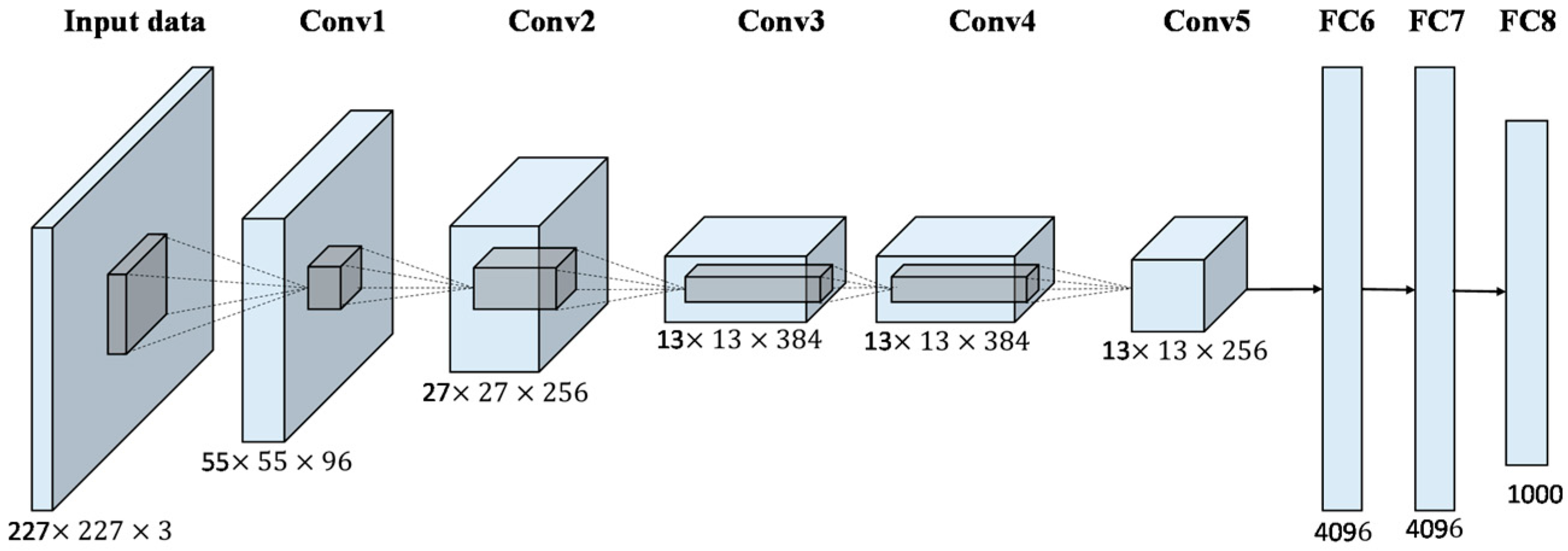
Figure 1: An illustration of the architecture of AlexNet, reprinted from [Han et al., 2017] with permission. The input layer is composed of 224$\times$224 units or the ‘retina’ (far left) that encodes images and feeds the activated visual pixels into the first convolutional layer (conv1). conv1 learns 11$\times$11 filters (a.k.a. features) that are repeated across the input every four pixels (a stride of 4). In conv1, there are 96 different filter banks that each code for a different feature in the input across multiple retinal locations, much like there are different simple cells that encode different line orientations across multiple retinal locations. Different convolutional layers have different size filters and different number of filter banks, with ‘max pooling’ layers (not depicted) occurring after the conv1, conv2, and conv5 layers. The output of conv5 is then fed into a series of three fully connected (fc) layers, with layers fc6 and fc7 each including 4096 units, and fc8 including 1000 units. Each unit in fc8 codes for a single category. A softmax function is applied at fc8 to give the output probabilities for each learned category, in a localist or ‘one hot’ encoding scheme. We recorded from units in conv5, fc6 and fc8.

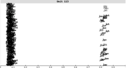
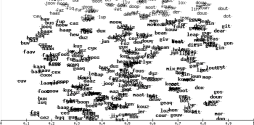
Figure 2: Top left: jitterplot of unit 113 in an RNN (under the superposition constraint) selective to the letter ‘j’ [Bowers et al., 2016]. Top centre: jitterplot of a non-selective unit 160 found in an RNN trained on words one-at-a-time from [Bowers et al., 2016]. Top right: Activation maximization image of unit conv5.9 AlexNet that resembles a lighthouse [Nguyen et al., 2016a]. Bottom: highest-activation images for a ‘lamp’ detector with .84 $precision$in the layer conv5 of AlexNet; from [Zhou et al., 2015].

Here we compare a range of measures of selectivity on a number of different convolutional networks of object identification, but focus on AlexNet [Krizhevsky et al., 2012] trained on the ImageNet dataset [Deng et al., 2009] because many authors have studied the selectivity of single hidden units in this model using a range of quantitative [Zhou et al., 2018a, 2015] and qualitative [Nguyen et al., 2015, Yosinski et al., 2015a, Simonyan et al., 2013] methods. AlexNet is one of the first modern DCNNs, and its dramatic success in categorizing images from ImageNet (that includes over 1 million images of objects and animals taken from 1000 categories) is often credited with starting the modern era of NN research. Its architecture is given in Figure 1. The network includes alternating convolutional and pooling layers from the input up to 5^th convolutional or ‘conv5’ layer. The convolutions are spatially organized learned filters (single units) that encode features within their receptive field, with each filter repeated across multiple spatial locations (analogous to a simple cell in V1 that encodes for a feature in its receptive field – something like a line of a specific orientation – with equivalent simple cells coding for the same orientation repeated over retinal locations). Following most of the convolutional layers in AlexNet is a pooling layer, in this case, max pooling, in which units take on the maximum activation value of a given convolutional filter in its receptive field (much like a complex cell in V1 that responds to the most active simple cell within a small retinotopic range). Together the convolutional and pooling layers learn useful visual features for object categorization. These features are input to layer fc6 that is the first of three fully connected layers (fc6, fc7 , fc8 ) with fc8 , after applying softmax, encoding all 1000 categories in a localist or ‘one hot’ coding manner (i.e. the ‘tiger sharks’ category is encoded by: [0,0,0,1,0…0]).

In the experiments reported below, we explored the selectivity for the learned object categories in the last three hidden layers of AlexNet, namely conv5 , fc6 and fc7 . We also assessed the selectivity of units in two more recent DCNNs, namely, VGG-16 and GoogLeNet models trained on the ImageNet and Places-365 dataset (over two million images that depict different scenes; e.g., kitchen, bedroom, forest, etc.). In these cases, we only consider a few units that were considered highly selective according to the Network Dissection method [Zhou et al., 2018a].

In order to directly compare and have a better understanding of the different selectivity measures, we assessed (1) localist, (2) $precision$, and (3) CCMAS selectivity, as well as a range of signal detection methods, namely, (4) recall with 100% and 95% precision, (5) maximum informedness, (6) specificity at maximum informedness, and (7) recall (also called sensitivity) at maximum informedness, and false alarm rates at maximum informedness (all described in Sec. 3). In addition to these quantitative measures, we assessed the human interpretation of images generated by a state-of-the-art activation maximization (AM) method [Nguyen et al., 2017] for units in layers conv5 , fc6, and fc8 layers as well as display jitterplots of some of the most selective units as determined by quantitative methods above. The jitterplots provide a more intuitive assessment of degree of selectivity that are usefully compared to the different quantitative and AM measures in order to get a better sense of these measures.

3 Methods

Network and Dataset All $\sim$1.3M photos from the ImageNet ILSVRC 2012 dataset [Deng et al., 2009] were cropped to $277\times 277$ pixels and classified by the pre-trained AlexNet CNN [Krizhevsky et al., 2012] shipped with Caffe [Jia et al., 2014], resulting in 721,536 correctly classified images. Once classified, the images are not re-cropped nor subject to any changes. To get the activations we fed the correct images into AlexNet and recorded the activations at that layer (futher details and full codebase available at: https://github.com/ellagale/testing_object_detectors_in_deepCNNs). We analyzed the fully connected (fc) layers: fc6 and fc7 (4096 units each), and the top convolutional layer conv5 which has 256 filters. We only recorded the activations of correctly classified images. The activation files are stored in .h5 format and are available at https://bristol.codersoffortune.net/AlexNet_Merged/. We randomly selected 233 conv5, 2738 fc6, 2239 fc7 units for analysis, amounting to around 90% of conv5, and roughly 60% of fc6 and fc7, numbers chosen owing to time constraints.

Localist selectivity Following Bowers et al. [2014], we define a unit to be localist for class $A$ if the set of activations for class $A$ was higher and disjoint with those of $\neg A$. Localist selectivity is easily depicted with jitterplots [Berkeley et al., 1995] in which a scatter plot for each unit is generated (see Figs. 2 and  4). Each point in a plot corresponds to a unit’s activation in response to a single image, and only correctly classified images are plotted. The level of activation is coded along the $x$-axis, and an arbitrary value is assigned to each point on the $y$-axis.

Precision $precision$refers to the proportion of items above some threshold from a given class. The $precision$method of finding object detectors involves identifying a small subset of images that most strongly activate a unit and then identifying the critical part of these images that are responsible for driving the unit. Zhou et al. [2015] took the 60 images that activated a unit the most strongly and asked independent raters to interpret the critical image patches (e.g., if 50 of the 60 images were labeled as ‘lamp’, the unit would have a$precision$index of 50/60 or .83; see Fig. 2). Object detectors were defined as units with a $precision$score $>$ .75: they reported multiple such detectors. Here, we approximate this approach by considering the 60 images that most strongly activate a given unit and assess the highest percentage of images from a given output class.

CCMAS Morcos et al. [2018] used a selectivity index called the Class-Conditional Mean Activation Selectivity (CCMAS). The CCMAS for class $A$ compares the mean activation of all images in class $A$, $\mu_{A}$, with the mean activation of all images not in class $A$, $\mu_{\neg A}$, and is given by: $\left(\mu_{A}-\mu_{\neg A}\right)/\left(\mu_{A}+\mu_{\neg A}\right)$. Here, we assessed class selectivity for the highest mean activation class.

Activation Maximization We harnessed an activation maximization method called Plug & Play Generative Networks (PPGNs) [Nguyen et al., 2017] in which an image generator network was used to generate images (AM images) that highly activate a unit in a target network.

Formally, we attempt to maximize the activation $\phi(.)$ of a neuron indexed $k$ at layer $l$ of a target neural network:

$$x^{*}=\mathrm{argmax}_{x}(\phi_{l,k}(x))$$ (1)

However, simply modifying an image pixel-wise in the direction of increasing neural activity often yields similar and noisy stimuli that are not human-interpretable Nguyen et al. [2019]. Therefore, PPGNs authors proposed to harness an image generator network $G$ as a strong natural image prior and search in the input space of generator $G$ for input vectors $z$ is in $R^{4096}$ such that the generated images $G(z)$ do not only (1) cause high neural activation but are also (2) realistic and (3) diverse Nguyen et al. [2017]. We used the public PPGN code released by Nguyen et al. [2017] and their default hyperparameters. That is, we generated each image by running an Stochastic Gradient Descent (SGD) optimizer for 200 steps with an initial learning rate of 1.0, and the multipliers for the realism, high-activation, and diversity terms are $10^{-5}$, 1, and $10^{-17}$, respectively. We generated 100 separate images that maximally activated each unit in the conv5, fc6, and fc8 layers of AlexNet. Images were used in the experiment described below (Sec. 4.2).

Recall with perfect and 95% precision Recall with perfect and 95%$precision$are related to localist selectivity except that they provide a continuous rather than discrete measure. For recall with perfect$precision$we identified the image that activated a given unit the most and counted the number of images from the same class that were more active than all images from all other classes. We then divided this result by the total number of correctly identified images from this class. A recall with a perfect$precision$score of 1 is equivalent to a localist representation. Recall with a 95%$precision$allows 5% false alarms.

Maximum informedness Maximum informedness identifies the class and threshold where the highest proportion of images above the threshold and the lowest proportion of images below the threshold are from that class [Powers, 2011]. The informedness is computed for each class at each threshold, with the highest value selected. Informedness summarises the diagnostic performance of unit for a given class at a certain threshold based on the recall $[\mathrm{TruePositives}/(\mathrm{TruePositives}+\mathrm{FalseNegatives})]$ and specificity $[\mathrm{TrueNegatives}/\mathrm{TrueNegatives}+\mathrm{FalsePositives})]$ in the formula $[\mathrm{informedness}=\mathrm{recall}+\mathrm{specificity}-1]$ [Powers, 2011].

Sensitivity or Recall at Maximum Informedness For the threshold and class selected by Maximum Informedness, recall (or hit-rate) is the proportion of items from the given class that are above the threshold. Also known as true postive rate.

Specificity at Maximum Informedness For the threshold and class selected by Maximum Informedness, the proportion of items that are not from the given class that are below the threshold. Also known as true negative rate.

False Alarm Rate at Maximum Informedness For the threshold and class selected by Maximum Informedness, the proportion of items that are not from the given class that are above the threshold.

Network Dissection Network Dissection Bau et al. [2017] is a method for assessing the selectivity of convolutional filter with respect to over a thousand visual concepts relating to scenes, objects, parts, materials, colours and textures as coded in the Broden dataset [Zhou et al., 2018a]. The Broden dataset contains 60000 real-world images, each with an accompanying concept-location map, coding at the pixel-level where a given concept occurs in the image. For example, if the concept is the colour ‘red’, all red pixels in the image will be labelled 1 on the concept-location map and all other pixels with be 0. Network Dissection compares the concept-location map for an image with the activation map of a convolutional filter in response to that image. This comparison is done using intersection over union (IoU):

$IoU=\frac{\mathrm{thenumberofpixellocationsthatare1inbothmaps}}{\mathrm{thetotalnumberofuniquepixelslabelled1inbothmaps}}$

If the IoU score is greater that .04, then the filter that produced the activation map is labelled as a detector for the labelled concept. Note, we did not carry out any network dissection analyses ourselves, but simply selected units that were considered object detectors according to this metric by Zhou et al. [2018a] in Section 3.3 and D.

Methodological details for the behavioral experiment One hundred generated images were made for units in hidden layers conv5 and fc6 and output layer fc8 in AlexNet, as in Nguyen et al. (2017), and displayed as $10\times 10$ image panels. We chose these three layers because they span across a wide spectrum of neural selectivity and two main types of layers: convolutional and fully-connected. conv5 were found to contain high-level object detectors (e.g., dog faces) in convolutional layers Bau et al. [2017], Zhou et al. [2014]. fc6 is a fully-connected layer that contain units often capture amalgamation of different concepts (i.e., a generalist rather localist neurons) Nguyen et al. [2016b]. fc8 neurons are trained specifically to light up for images of pre-defined categories and therefore are expected to exhibit a high degree of selectivity.

A total of 3,299 image panels were used in the experiment (995 associated with fc8 output units with 5 units omitted by mistake, all 256 conv5 units, and 2048 randomly selected fc6 image panels constituting half of all units in this layer) and were divided into 64 counterbalanced lists of 51 or 52 (4 conv5, 15 or 16 fc8 and 32 fc6). Fifty-one of the lists were assigned to 5 participants and 13 lists were assigned to 6 participants. The study was approved by the University of Bristol Faculty of Science Ethics Committee and informed consent was obtained from all participants.

To test the interpretability of these units, paid volunteers were asked to look at image panels and asked if the images had an object / animal or place in common, i.e. a concrete object. In training, they were also shown examples of panels that only included common abstract concepts, like ‘color’, ‘shape’ or ‘texture’, that required a ‘no’ for an answer. If the answer was ‘yes’, they were asked to name that object simply (i.e. fish rather than goldfish). For any units where over 80% of humans agreed that there was an object present, analyses of the common responses were carried out by reading the human responses and comparing them to both each other and to the output class labels. Agreement was taken if the object was the same rough class. For example, ‘beer’, ‘glass’, and ‘drink’ were all considered to be in agreement in the general object of ‘drink’, and in agreement with both the classes of ‘wine glass’ and ‘beer’ as these classes were also general drink classes (this is an actual example, most responses were more obvious and required far less interpretation than that). Participants were given six practice trials, each with panels of 20 images before starting the main experiment. Practice trials included images that varied in their interpretability. Analyses of common responses were done for any units where over 80% of humans agreed there was an object present. An illustration of the task can be found in Appendix A, and readers can test themselves at: https://research.sc/participant/login/dynamic/63907FB2-3CB9-45A9-B4AC-EFFD4C4A95D5. All materials used in the AM experiment are stored here: https://gorilla.sc/openmaterials/84689.

4 Results

4.1 Comparison of selectivity measures in AlexNet

a. Precision	b. No. of classes in top 100	c. CCMAS
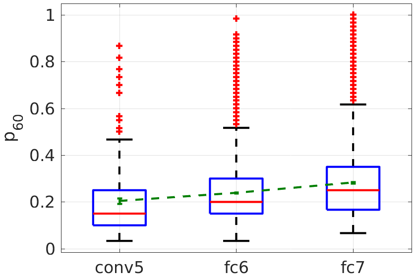
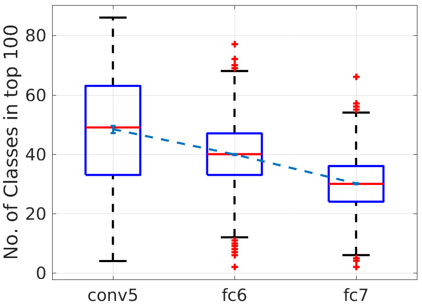
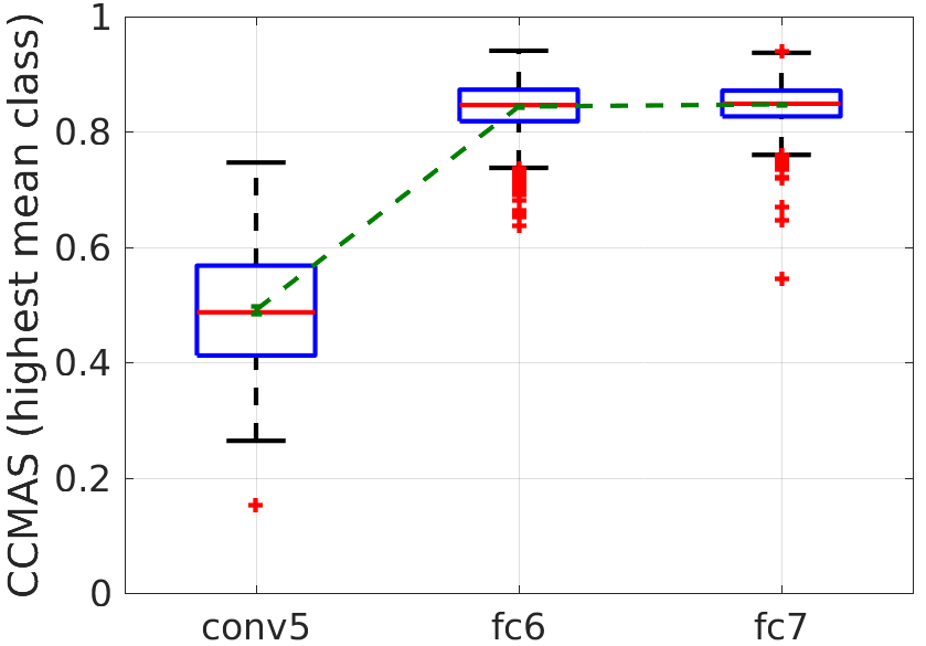
d. Recall (precision = 1)	e. Recall (precision = 0.95)	f. Max. informedness
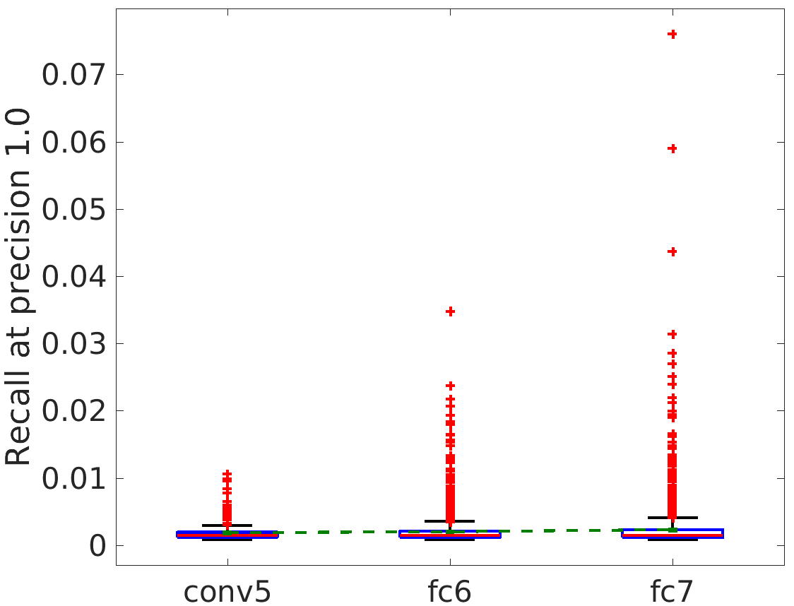
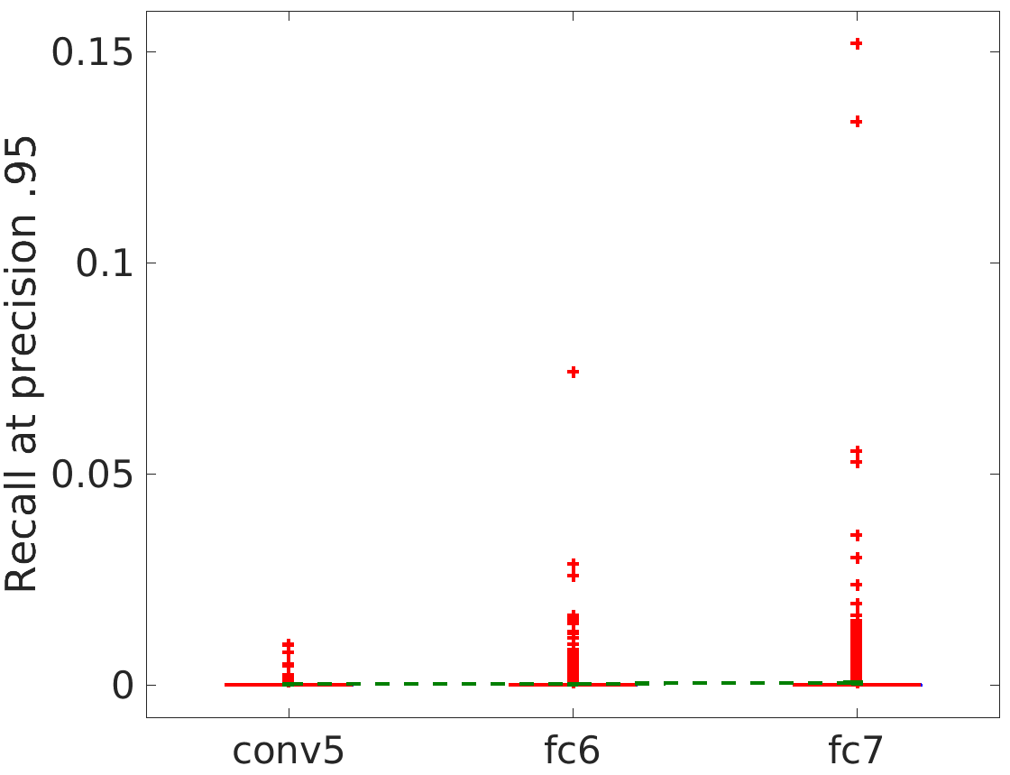
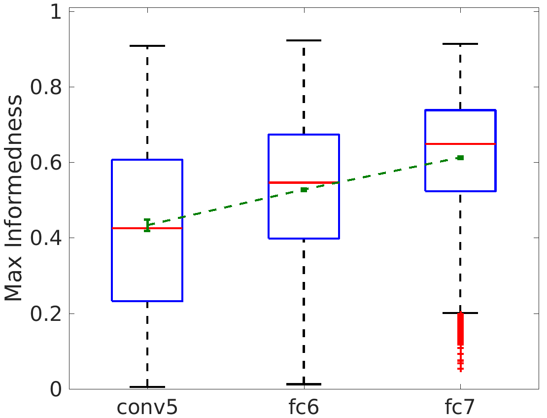
g. Specificity	h. Recall	i. False alarm proportion
(at max. informedness)	(at max. informedness)	(at max. informedness)

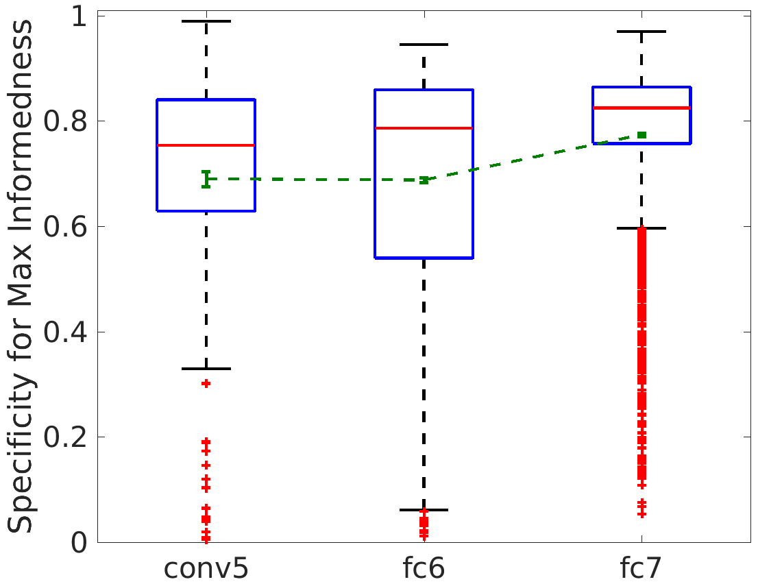
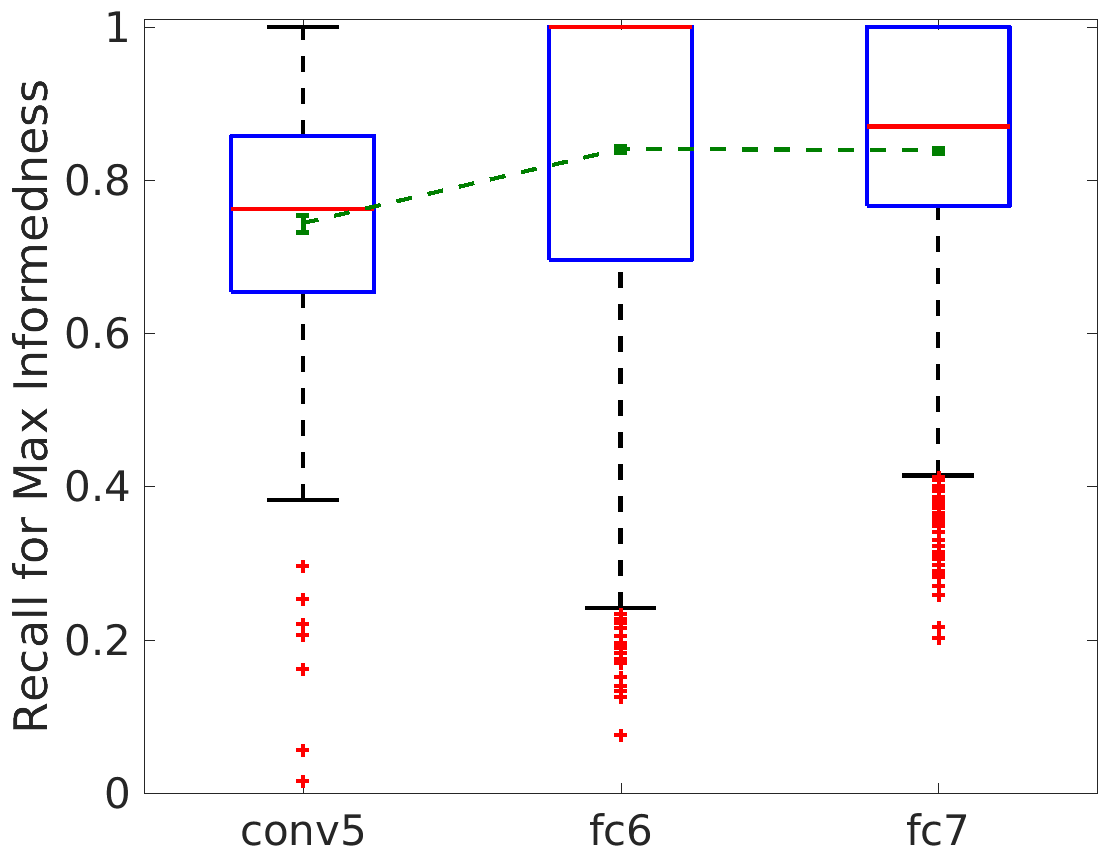
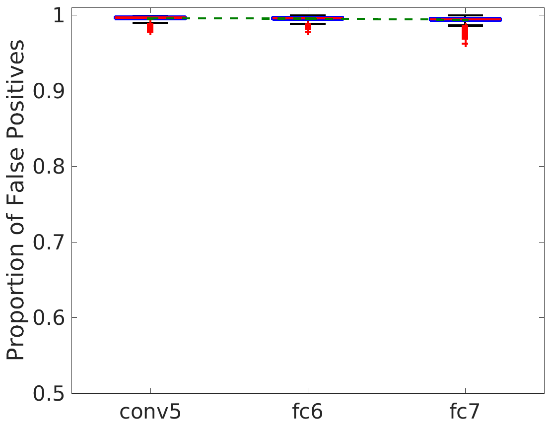
Figure 3: Different selectivity measures across the conv5, fc6, and fc7 layers of AlexNet. Red-line: median of data, top and bottom of box edges is the 25^th and 75^th percentile, whiskers extend to extreme edges of distribution not considered outliers and red crosses are outliers. Green points and dashed lines are the means of the distributions with standard errors. The high levels of selectivity observed with the $precision$and CCMAS measures are in stark contrast with the low levels of selectivity observed with the recall with perfect$precision$and high false-alarm rates at maximum informedness. Note the y-axis scaling for panels 3e, f, and i are different from other panels in order to depict the findings more clearly.

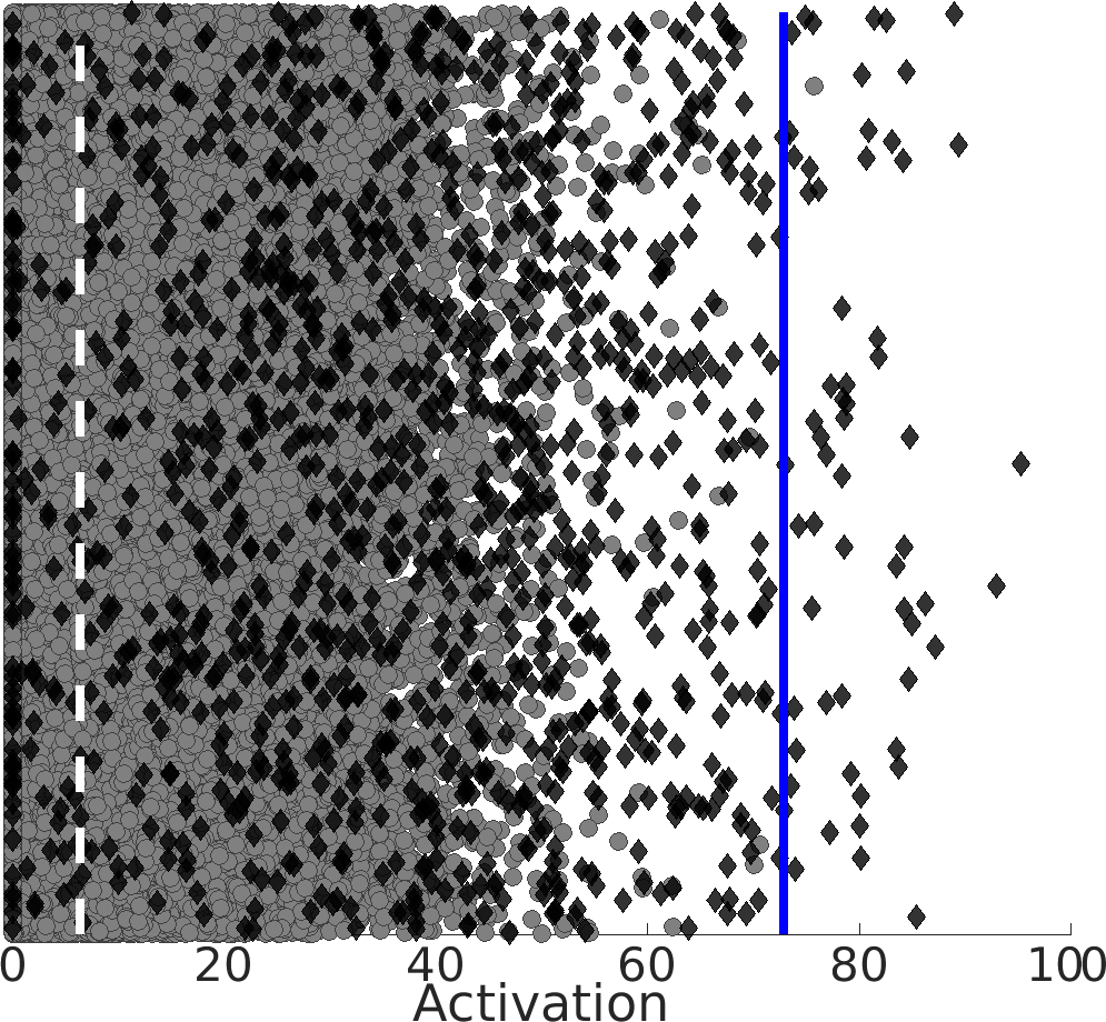
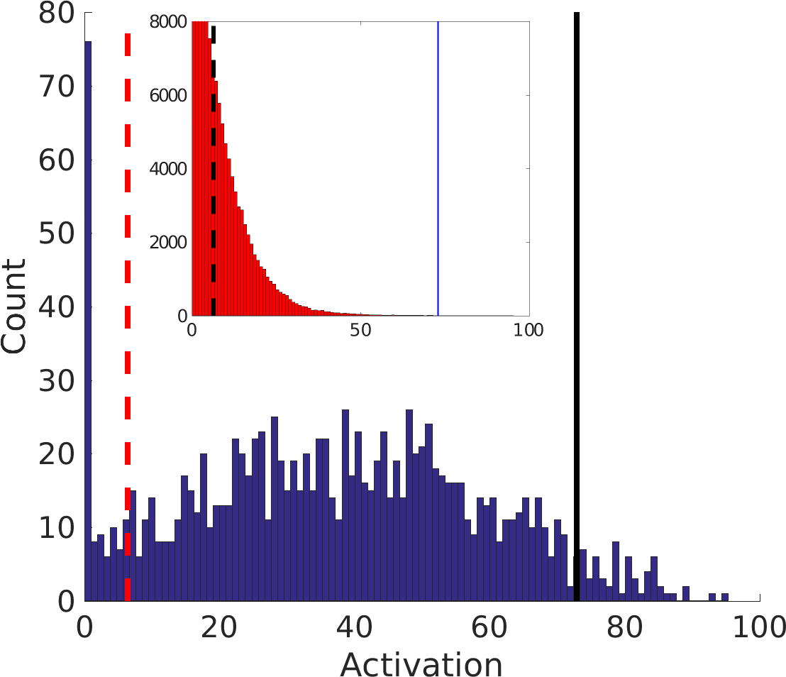
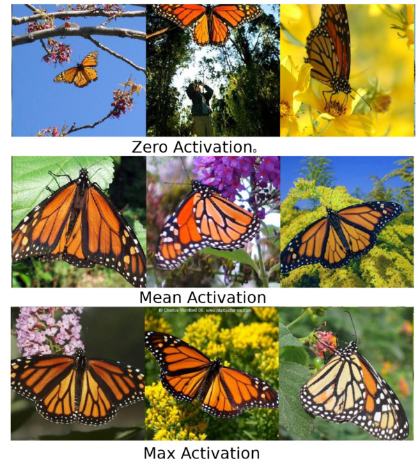
Figure 4: Data for unit fc6.1199. Left: activation jitterplot, black diamonds: Monarch butterfly images; grey circles: all other classes; white dashed line: threshold for the butterfly class maximum informedness; blue solid line: threshold for top 60 activations. Middle: histogram of activations of Monarch butterflies; red dashed line: threshold for the butterfly class maximum informedness; black solid line: threshold for top 60 activations. Inset: zoomed-in histogram of all activations across all ImageNet classes of unit fc6.1199 (N.B. this plot shows only the highest 121,586 activations; there are 596,734 activations at 0). There are Monarch butterfly images covering the whole range of values, with 72 images (5.8% of the total) having an activation of 0. Right: example ImageNet images with activations of 0 (top), the mean, 39.2$\pm$0.6, (middle), and the maximum, 95, (bottom) of the range. Although the high $precision$score suggests that this unit is a butterfly detector this is misleading given there are butterfly images over the entire activation range (including 0).

The results from the various selectivity measures applied to the conv5, fc6, and fc7 layers of AlexNet are displayed in Fig. 3a–i. We did not plot the localist selectivity as there were no localist ‘grandmother units’. The first point to note is that multiple units in the fc6 and fc7 layers had $precision$and CCMAS scores approaching 1.0. For example, in layer fc7, we found 14 units with a $precision$> 0.9, and 1487 units with a CCMAS > 0.9. The second point is that other measures highlight much reduced estimates of selectivity. For example, unit fc7.255 had a CCMAS of .9 and a$precision$of .97, but its recall with a perfect $precision$score was only .08, meaning that there was at least one non-Monarch butterfly image more strongly activated than 92% of the Monarch butterfly images (and this was the highest recall with a perfect $precision$score in the model). A similar pattern of results was observed with recall with .95 precision, as shown in panel 3e.

The unit with the top maximum informedness score (unit 3290 also responding to images of Monarch butterflies with a score of 0.91) had a false alarm rate above its optimal threshold > 99% (indeed the minimum false alarm rate for any unit was 0.96). This means that over 99% of images that activate this unit above its ideal threshold for detecting Monarch butterflies, are not Monarch butterflies.

To illustrate the contrasting measures of selectivity consider unit fc6.1199 depicted in Fig. 4 that has a$precision$score of .98 and a CCMAS score of .92. By Zhou et al.’s criterion, this is a ‘Monarch Butterfly’ detector (its $precision$score is > .75). The Maximum Informedness score was .82, and again > 99% of images active above this threshold (white dashed line in Fig. 4) were false alarms. A more conservative threshold would reduce the false alarm rate. For example, setting a threshold below the 60 most active items (blue solid line denoting the the $precision$measure threshold) has a false alarm rate of .02. However, only 59 of the 1241 Monarch butterflies are above this threshold (e.g., sensitivity of .05). Maximum Informedness scores reflect the trade off between false alarms and false negatives, and as such, gives a lower selectivity score to this unit.

4.2 Human interpretation of Activation Maximization images for AlexNet units

Activation Maximization is one of the most commonly used interpretability methods for explaining what a single unit has learned in many artificial CNNs and even biological neural networks (see Nguyen et al. [2019] for a survey). Our behavioral experiment provides the first quantitative assessment of AM images and compares AM interpretability to other selectivity measures.

Table 1: Human judgements of whether AM images look like familiar objects in layers conv5, fc6, and fc8 in AlexNet. Standard error shown in parenthesis.

layer	% ‘yes’	% units $\geq$ 80%	% overlap between humans and:
	responses	‘yes’ response	humans	most active	CCMAS
	(a)	(b)	(c)	object (d)	class (e)
conv5	21.7 ($\pm$1.1)	4.3 ($\pm$ 1.3)	89.5 ($\pm$5.7 )	34.1 ($\pm$14.4)	0
fc6	21.0 ($\pm$0.4)	3.1 ($\pm$ 0.4)	80.4 ($\pm$4.1)	23.3 ($\pm$5.9)	18.9 ($\pm$5.9)
fc8 (Output)	71.2 ($\pm$0.6)	59.3 ($\pm$1.6)	96.5 ($\pm$0.4)	95.4 ($\pm$0.6)	94.6 ($\pm$0.7)

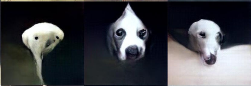
(a) conv5.183

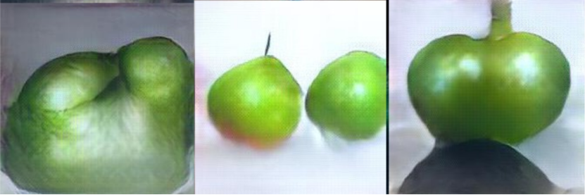
(b) fc6.319

(c) fc8.969

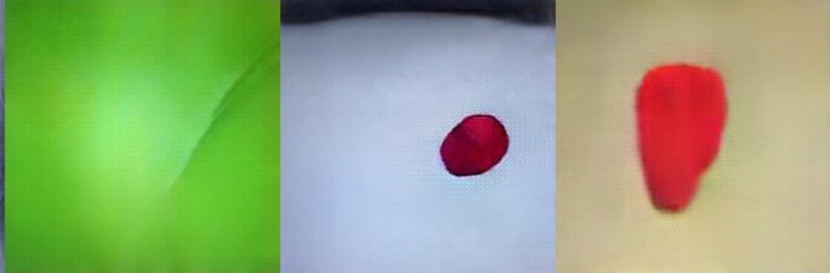
(d) conv5.65

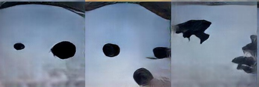
(e) fc6.103

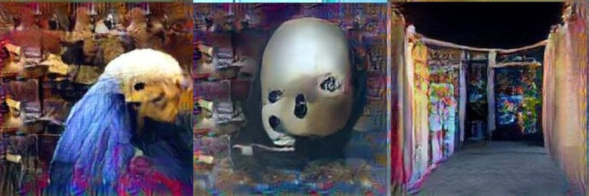
(f) fc8.865

Figure 5: Example AM images that were either judged by all participants to contain objects (a–c) or to be uninterpretable as objects (d–f). The human label for unit conv5.183 (a) was ‘dogs’; the most active image was of a ‘flat-coated retriever’; CCMAS class was ‘monitor’. For fc6.319 (b), subjects reported ‘green peppers’ or ‘apples’ (all classified as the same broad class in our analysis); both the most active item and CCMAS class were ‘Granny Smith apples’. For fc8.969 (c), humans suggested ‘beverage’ or ‘drink’; both the most active item and CCMAS class were ‘eggnog’.

The results are summarized in Table 1. Not surprisingly, the AM images for output fc8 units are the most human-recognizable as objects across the AlexNet layers (71.2%; Table 1a). In addition, when they were given a consistent interpretation, they almost always (95.4%; Table 1d) match the corresponding ImageNet category. By contrast, less than 5% of units in conv5 or fc6 were associated with consistently interpretable images (Table 1b), and the interpretations only weakly matched the category associated with the highest-activation image or CCMAS selectivity (Table 1d–e). Apart from showing that there are few interpretable units in the hidden layers of AlexNet, our findings show that the interpretability of images does not imply a high level of selectivity given the signal-detection results (Fig. 2d–h). See Fig. 5 for an example of the types of images that participants rated as objects or non-objects.

4.3 Comparing selectivity measures in other CNNs

Thus far we have assessed the selectivity of hidden units in AlexNet and shown that no units can reasonably be characterized as object detectors despite the high$precision$and CCMAS scores of some units. This raises the question as to whether more recent CNNs learn object detector units. In order to address this, we display jitterplots for three units that have the highest IoU scores according to the Network Dissection for the category BUS in (a) GoogLeNet trained on ImageNet, (b) GoogLeNet trained on Places-365, and (c) VGG-16 trained on Places-365, respectively [Zhou et al., 2018a], see figure 6. Models trained on the Places-365 dataset learn to categorize images into scenes (e.g., bedrooms, kitchens, etc.) rather than into object categories, and nevertheless, Zhou et al. [2018a] reported more object detectors in models trained on the Places-365 dataset (e.g., selective for objects within a scene such as a lamp in a bedroom or a car on a highway) than for ImageNet. We illustrate the selectivity of the BUS category because it corresponds to three output categories in ImageNet so we can easily plot the jitterplots for these units.

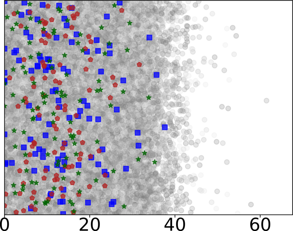
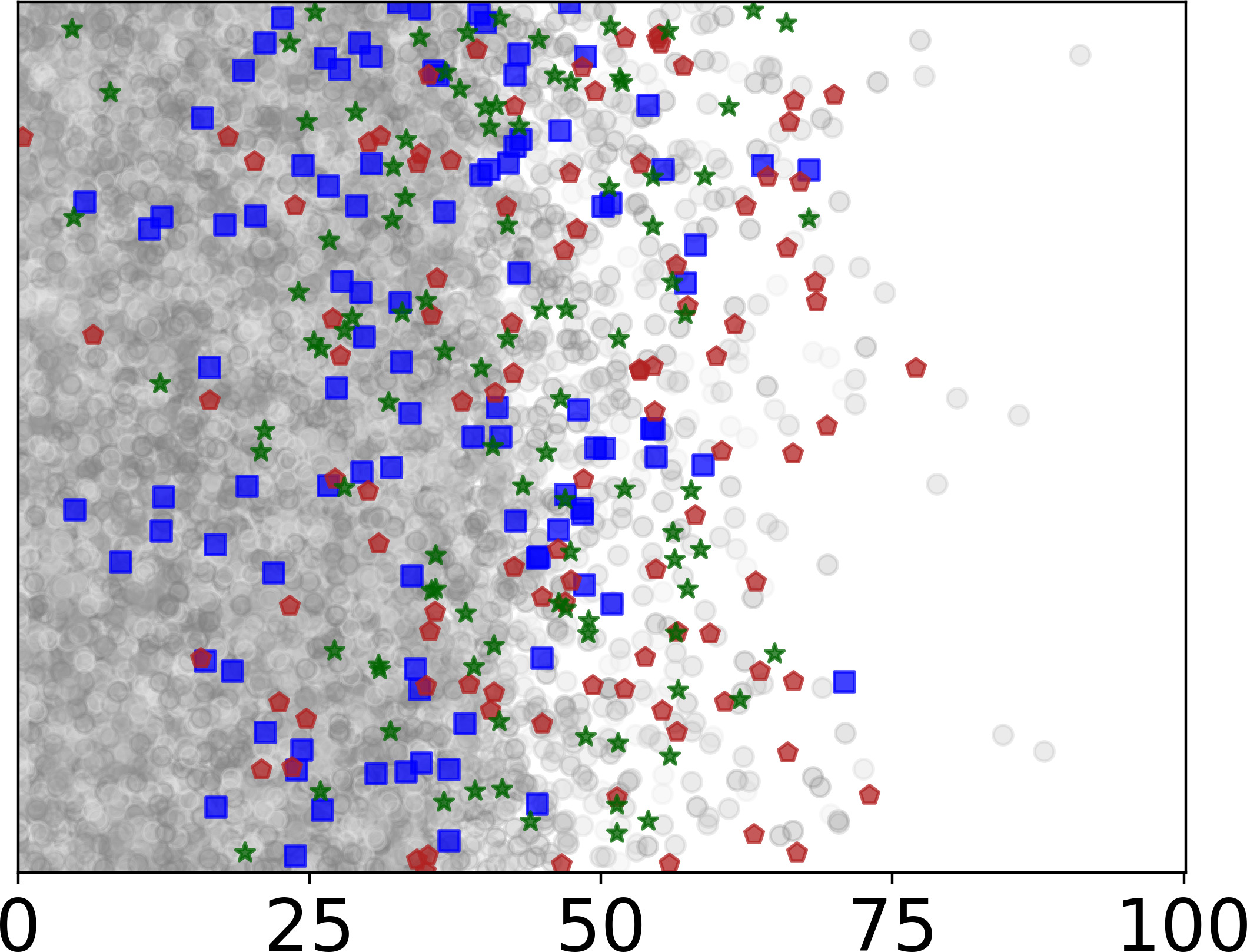
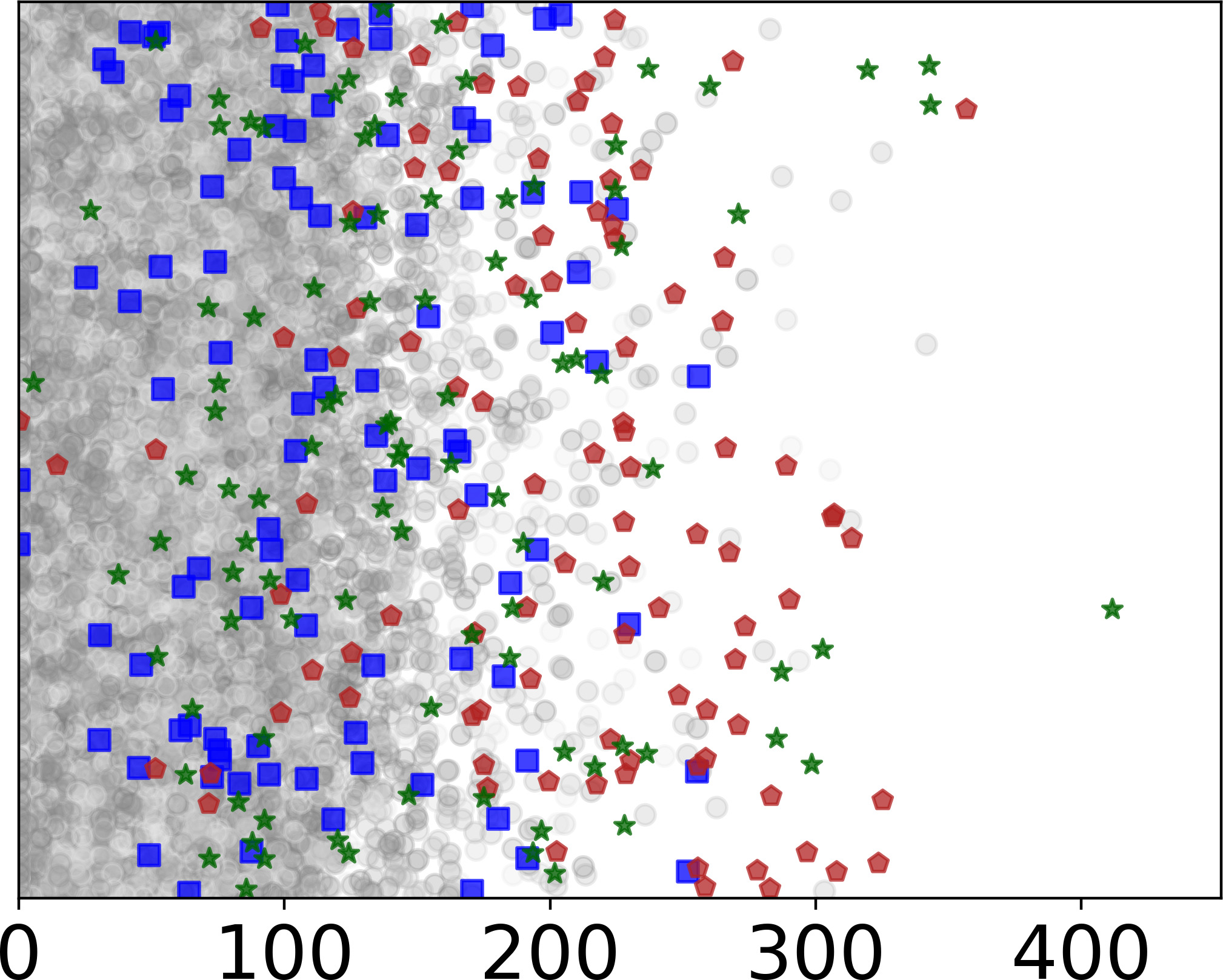
a. GoogLeNet (ImageNet)	b. GoogLeNet (Places-365)	c. VGG-16 (Places-365)
inception4e.494	inception4e.824	conv5_3.20
$precision$: 0.0	$precision$: 0.27	$precision$: 0.53
CCMAS:0.52	CCMAS: 0.55	CCMAS: 0.82
$\mu_{A}$ = 72.5   $\mu_{\neg A}$ = 22.8	$\mu_{A}$ = 41.0   $\mu_{\neg A}$ = 11.8	$\mu_{A}$ = 157.6   $\mu_{\neg A}$ = 15.2

Figure 6: The units with with the highest Network Dissection scores for the category ‘bus’. The scatter plots, $precision$, and CCMAS scores all indicate a low selectivity for this category. blue squares: ‘school bus’; red pentagons: ‘trolleybus’; green stars: ‘minibus’; grey circles: other classes.

As was the case with AlexNet, the jitterplots show that the most selective units display some degree of selectivity, with the BUS images more active on average compared to non-Buses. However, these units are no more selective than the units we observed in AlexNet. Indeed, the $precision$measure of selectivity for the first units is 0.0, with none of the three units having a $precision$of .75 that was the criterion of object detectors by Zhou et al. [2015], and CCMAS scores for first two units were roughly similar to the mean CCMAS score for AlexNet units in conv5 (and much lower than the mean in fc6 and fc7 ). The most selective VGG-16 unit trained on Places-365 has lower $precision$and CCMAS scores than the Monarch Butterfly unit depicted in Figure 3. So again, different measures of selectivity support different conclusions, and even the most selective units are far from the selective units observed in recurrent networks as reported in Figure 1a. See Tables A3 - A5 in Appendix D for more details about these and other units.

5 Discussions and Conclusions

Our central finding is that different measures of single-unit selectivity for objects support very different conclusions when applied to the same units in AlexNet. In contrast with the $precision$[Zhou et al., 2015] and CCMAS [Morcos et al., 2018] measures that suggest some highly selective units for objects in layers conv5, fc6, and fc7, the recall with perfect $precision$and false alarm rates at maximum informedness show low levels of selectivity. Indeed, the most selective units have a poor hit-rate or a high false-alarm rate (or both) for identifying an object class. The same outcome was observed with units in VGG-16 and GoogLeNet trained on either ImageNet or the Places-365 dataset.

Not only do the different measures provide very different assessments of selectivity, the $precision$, CCMAS, and Network Dissection measures provide misleading estimates of selectivity that have led to mistaken conclusions. For example, unit fc6.1199 in AlexNet trained on ImageNet is considered an Monarch Butterfly detector according to Zhou et al. [2015] with a $precision$score of .98 (and a CCMAS score of .93). But the jitterplot in Fig. 3 and signal detection scores (e.g., high false alarm rate at maximum informedness) show this is a mischaracterisation of this unit. In the same way, the Network Dissection method identified many object detectors in VGG-16 and GoogLeNet CNNs, but the jitterplots in Fig. 6 show that this conclusion is unjustified.

What level of selectivity is required before a unit can be considered an ‘object detector’ for a given category? In the end, this is a terminological point. On an extreme view, one might limit the term to the ‘grandmother units’ that categorize objects with perfect recall and specificity, or alternatively, it might seem reasonable to describe a unit as a detector for a specific object category if there is some threshold of activation that supports more hits than misses (the unit is strongly activated by the majority of images from a given category), and at the same time, supports more hits than false alarms (the unit is strongly activated by items from the given category more often than by items from other categories). Or perhaps a lower standard could be defended, but in our view, the term ‘object detector’ suggests a higher level of selectivity than 8% recall at perfect precision. That said, our results show that some units respond strongly to some (unknown) features that are weakly correlated with an object category. For instance, unit fc6.1199 is responding to features that occur more frequently in Monarch Butterflies than other categories. This can also be seen in a recent ablation study in which removing the most selective units tended to impair the CNN’s performance in identifying the corresponding object categories more than other categories [Zhou et al., 2018b]. But again, the pattern of performance is not consistent with the units being labeled ‘object detectors’.

What should be made of the finding that localist representations are sometimes learned in RNNs (units with perfect specificity and recall), but not in AlexNet and related CNNs? The failure to observe localist units in the hidden layers of these CNNs is consistent with Bowers et al. [2014]’s claim that these units emerge in order to support the co-activation of multiple items at the same time in short-term memory. That is, localist representations may be the solution to the superposition catastrophe, and these CNNs only have to identify one image at a time. The pressure to learn highly selective representations in response to the superposition constraint may help explain the reports of highly selective neurons in cortex given that the cortex needs to co-activate multiple items at the same time in order to support short-term memory [Bowers et al., 2016].

At the same time, it should be emphasized that the RNNs that learned localist units were very small in scale compared to CNNs we have studied here, and accordingly, it is possible that the contrasting results reflect the size of the networks rather than the superposition catastrophe per se. Relevant to this issue a number of authors have reported the existence of selective units in larger RNNs with long-short term memory (LSTM) units [Karpathy et al., 2016, Radford et al., 2017, Lakretz et al., 2019, Na et al., 2019]. Indeed, Lakretz et al. [2019] use the term ‘grandmother cell’ to describe the units they observed. It will be interesting to apply our measures of selectivity to these larger RNNs and see whether these units are indeed ‘grandmother units’. It should also be noted that there are recent reports of impressively selective representations in generative adversarial networks [Bau et al., 2019] and variational autoencoders [Burgess et al., 2018] where the superposition catastrophe is not an issue. Again, it will be interesting to assess the selectivity of these units according to signal detection measures in order to see whether there are additional computational pressures to learn highly selective or even grandmother cells. We will be exploring these issues in future work.

Finally, how do these findings relate to the selectivity of neurons in visual cortex? Is the limited degree of selectivity observed in various CNNs a problem for the claim that these models provide a good theory of human vision? Not necessarily. As noted at the start, there is currently a debate about how selective neurons are in cortex, and few researchers have carried out relevant behavioral experiments that can be compared to the selectivity studies carried out in CNNs [Bowers et al., 2019]. Furthermore, there is widespread confusion about what constitutes a localist grandmother cell, with some versions of localist units responding to multiple different categories, with one category more active than all others. [Gubian et al., 2017]. This makes it all the more challenging to determine whether the human visual system learns to identify objects on the basis of localist codes. Nevertheless, a better understanding of the selectivity of units in CNNs and other artificial networks is a necessary step towards a better understanding of the relation between these models and human visual system. And adopting a standard set of measures will allow researchers to compare selectivity across different network architectures trained on different tasks in order to better understand the factors that contribute to more or less selectivity.

Appendix

Appendix A Instructions for behavioral experiment

Participants were provided the following instructions: "In each trial, a grid of computer generated images will be presented which may have recognisable common objects (e.g. car, trash can, banjo, clothes), animals (fish, bird, dog), or places (theatre, viaduct, volcano). In each trial, you will be asked whether you can identify multiple examples of an everyday object, place or animal." The full set of instructions, together with all of the stimuli used in the task are stored here: https://gorilla.sc/openmaterials/84689 and more details of the task are described under ‘Methodological details for the behavioral experiment’ in Section 3 of the manuscript. Below is a screen shot from an example trial where they were asked three questions of actual images.

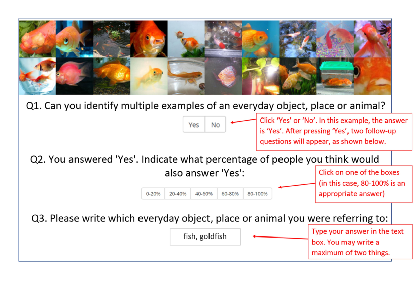
Figure A1: Example screen from the identification task shown to participants as part of the instructions. The images included on this practice trial are ImageNet2012 images, not AM images.

Appendix B Further data on the selectivity measures across AlexNet

Table  A1 gives the highest values of CCMAS and $precision$for each layer in AlexNet, with the corresponding CCCMAS and $precision$scores for these units. It is worth noting that the highest CCMAS score of all hidden units was .94 (fc7.31), which at first glance suggests that this unit is close to ‘perfect’ selectivity. However, this unit only has low a $precision$score of .11. (Note: $precision$in this analysis used the 100 most active items, rather than the 60 most active items). In other words, although the mean activation for the given class is very high relative to the mean of all other activations (high CCMAS), the proportion of items from that class in the 100 most active items is low (low $precision$). See C for some discussion of how this might occur.

LAYER.UNIT	CCMAS	Precision
Top CCMAS units
output.322	0.991	1.0
fc7.31	0.94	.11
fc6.582	0.93	.01
conv5.78	0.75	.05
Top $precision$units
output.0	0.99	1.0
fc7.255	0.90	.97
fc6.1199	0.92	.95
conv5.0	0.55	.77

Table A1: The units with the highest CCMAS and $precision$scores in AlexNet. Unit fc6.1199 was displayed in Fig. 4.

Table  A2 shows positive correlations between four of the selectivity measures used. There are moderate positive correlations between $precision$and CCMAS; and between $precision$and Recall at 95% precision. The other correlations between selectivity measures have weak positive correlations. All four selectivity measures are negatively correlated with the number of classes present in the 100 most active items, that is, the more selective the unit, the fewer classes will be represented in the most active 100 items.

	CCMAS	recall|0.95	Max. Inf.	No. classes in top100
$precision$	0.38	0.30	0.15	-0.68
CCMAS		0.09	0.14	-0.47
recall|0.95			0.10	-0.19
Max. Inf.				-0.22

Table A2: The correlations between the different measures. (All p’s < .001)

Appendix C Further issues with the CCMAS measure

The CCMAS measure is based on comparing the mean activation of a category with the mean activation for all other items, and this is problematic for a few reasons. First, in many units a large proportion of images do not activate a unit at all. For instance, our butterfly ‘detector’ unit fc6.1199 has a high proportion of images with an activation of 0.0 (see figure  4). Indeed, the inset on the middle figure shows that the distribution can be better described by exponential-derived fits rather than a Gaussian. This means that the CCMAS selectivity is heavily influenced by the the proportion of images that have an activation value of zero (or close to zero). This can lead to very different estimates of selectivity for CCMAS and $precision$or localist selectivity, which are driven by the most highly activated items.

In Figure  A2 we generate example data to highlight ways in which CCMAS score may be non-intuitive. In subplot (a) we demonstrate that a unit can have a CCMAS score of of 1.0 despite only a single item activating the unit. The point that we wish to emphasise is that a high CCMAS score does not necessarily imply selectivity for a given class, but might in fact relate to selectivity for a small subset of items from a given class, and this is especially true when a unit’s activation is sparse (many items do not activate the unit). However, the reverse can also be true. In subplot (c) we demonstrate that a unit can have a very low CCMAS score of .06 despite all of the most active items being from the same class.

In addition, if the CCMAS provided a good measure of a unit’s class selectivity, then one should expect that a high measure of selectivity for one class would imply that the unit is not highly selective for other classes. However, the CCMAS score for the most selective category and the second most selective category (CCMAS2) were similar across the conv5 , fc6 and fc7 . layers, with the mean CCMAS scores .491, .844, and .848, and the CCMAS2 scores .464, .821, .831. For example, unit fc7 .0 has a CCMAS of .813 for the class ‘maypole’, and a CCMAS2 score of .808 for ‘chainsaw’ (with neither of these categories corresponding ‘orangutan’ that had the highest $precision$of score of .14).

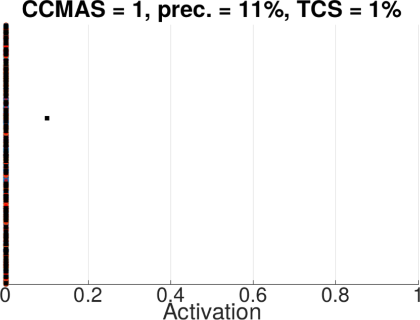
(a) One active item from one class.
CCMAS = 1
$precision$= .11

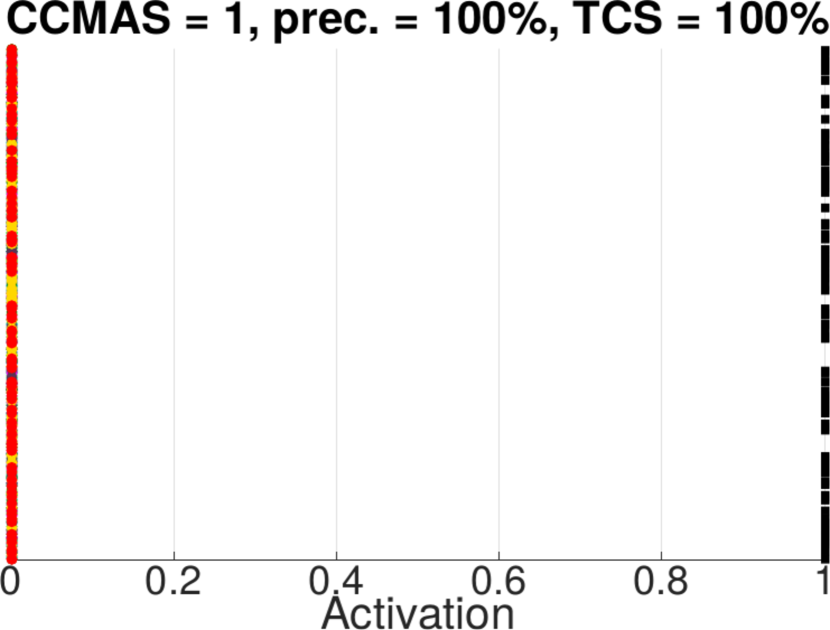
(b) Archetypal ‘GMC’ unit.
CCMAS = 1
$precision$= 1.0

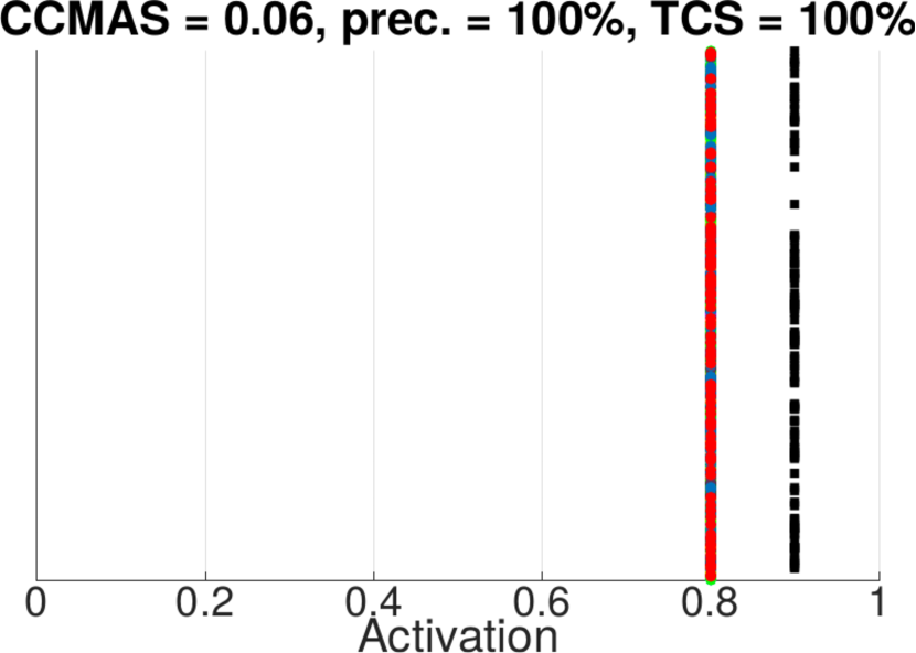
(c) One class more active than the others.
CCMAS = 0.06
$precision$= 1.0

Figure A2: Example of where the CCMAS does not match intuitive understandings of selectivity. Generated example data: (a) If a unit is off to all but a single image from a large class of objects, the CCMAS for that class is 1 (maximum possible selectivity). (b) An archetypal ‘grandmother’ cell (GMC), where the unit is strongly activated to all members of one class and off to everything else. The CCMAS is the same for (b) as for (a) although the $precision$is vastly different. (c): If a unit has high activations for all classes, but one class (black squares) is 0.1 more than all others (coloured circles), the CCMAS is very low (0.06) despite being 1.0 precision. The generated examples are for 10 classes of 100 items

Appendix D Testing units in other models

To investigate units characterized by Zhou et al. [2018a] to be object detectors, we focus on units from a single layer that are reported to be ‘bus detectors’, that is, units with an IoU $\geq.04$. We used the first 100 images per class from the ImageNet 2012 dataset as our test data. There are three classes of bus in this dataset: ‘n04146614 school bus’, ‘n04487081 trolleybus, trolley coach, trackless trolley’, ‘n03769881 minibus’, and this corresponded to 300 items out of 100000 images. Data for all bus unit detectors for VGG trained on places 365 are shown in table A3; for GoogLeNet trained on places 365 in table A4; and for GoogLeNet trained on ImageNet are shown in table A5. Note that for all units there are very few busses with activation at zero and that the mean activation for busses is higher than the mean activation for non-busses. However, all $precision$scores are all below .6, meaning that of the 100 items that most strongly activated the unit, at least 40 of them were not busses. Together these results suggests that whilst these units demonstrate some sensitivity to busses, they show poor specificity for busses (e.g., high false-alarm rate).

unit	IoU	top-4 match	no.$a_{x}$>0	no.$a_{x}$>0	$\mu_{A}$	$\mu_{\neg A}$	$precision$	CCMAS
			$x\in A$	$x\in\neg A$
conv5_3${}_{1}91$	.15	Y	99.0%	63.9%	131.9	16.1	.45	.78
conv5_3${}_{2}0$	.15	Y	99.0%	49.1%	157.6	15.2	.53	.82
conv5_3${}_{3}33$	.08	Y	99.0%	71.4%	101.7	17.5	.24	.71
conv5_3${}_{1}45$	.07	Y	97.3%	61.7%	75.5	12.5	.19	.72
conv5_3${}_{1}13$	.06	N	97.4%	41.0%	62.8	9.1	.12	.75
conv5_3${}_{4}43$	.04	N	95.3%	38.2%	59.3	8.1	.12	.76
conv5_3${}_{1}31$	.04	N	93.7%	22.3%	54.0	5.86	.08	.80

Table A3: Selectivity measures for VGG-16, trained on Places-365, top convolutional layer units identified by Zhou et al. [2018a] as object detectors. Standard errors not shown for space, but were below $\pm 5$. The IoU is from Zhou et al. [2018a]’s network dissection method. no.$a_{x}$>0 and no.$a_{x}$>0 $x\in A$ refer to the proportion of activations that were greater than zero for busses and non-busses respectively. $\mu_{A}$ and $\mu_{\neg A}$ are the class means for busses and non busses respectively. A unit was coded as top-4 match (Y) if there was a single bus in the 4 example pictures on the website (http://netdissect.csail.mit.edu/dissect/vgg16_places365/), and (N) if not.

unit	IoU	top-4 match	no.$a_{x}$>0	no.$a_{x}$>0	$\mu_{A}$	$\mu_{\neg A}$	$precision$	CCMAS
			$x\in A$	$x\in\neg A$
${}_{8}24$	.17	Y	100.0	91.4	41.0	11.8	.27	.55
${}_{7}45$	.13	Y	98.3	74.8	34.8	11.4	.06	.51
${}_{7}91$	.11	Y	98.3	71.4	32.7	5.3	.41	.72
${}_{1}94$	.11	N	100.0	85.3	26.6	8.8	.02	.51
${}_{8}2$	.11	Y	100.0	97.3	26.7	10.9	.14	.42
${}_{7}36$	.11	N	100.0	78.8	38.7	9.9	.05	.59
${}_{6}63$	.10	N	96.0	38.0	33.4	3.7	.15	.80
${}_{9}4$	.10	Y	100.0	91.6	38.3	9.5	.35	.60
${}_{7}72$	.08	N	97.3	54.6	21.7	5.2	.00	.61
${}_{1}13$	.08	N	100.0	88.0	24.9	9.2	.02	.46
${}_{7}08$	.06	N	100.0	85.1	29.7	9.1	.02	.53
${}_{8}01$	.06	N	100.0	64.5	35.2	6.4	.14	.69
${}_{1}99$	.06	N	99.7	92.2	21.5	7.7	.09	.47
8	.05	N	99.7	83.5	18.5	7.3	.01	.43
${}_{1}21$	.05	N	100.0	90.4	17.9	8.9	.01	.34
${}_{6}22$	.05	Y	96.0	65.0	27.5	6.4	.20	.62
${}_{9}7$	.04	Y	99.3	86.4	21.1	9.3	.04	.39

Table A4: Selectivity measures for GoogLeNet, trained on Places-365, layer inception4e units identified by Zhou et al. [2018a] as object detectors. Standard errors not shown for space, but were below $\pm 2$. The IoU is from Zhou et al. [2018a]’s network dissection method. A unit was coded as top-4 match (Y) if there was a single bus in the 4 example pictures on the website (http://netdissect.csail.mit.edu/dissect/googlenet_places365/), and (N) if not. no.$a_{x}$>0 and no.$a_{x}$>0 $x\in A$ refer to the proportion of activations that were greater than zero for busses and non-busses respectively. $\mu_{A}$ and $\mu_{\neg A}$ are the class means for busses and non busses respectively.

unit	IoU	top-4 match	no.$a_{x}$>0	no.$a_{x}$>0	$\mu_{A}$	$\mu_{\neg A}$	$precision$	CCMAS
			$x\in A$	$x\in\neg A$
${}_{4}94$	.11	N	99.0	82.4	72.5	22.8	.00	.52
${}_{8}28$	.10	Y	100.0	72.6	109.4	17.6	.45	.72
${}_{5}69$	.10	Y	99.7	85.9	74.9	20.0	.05	.58
${}_{3}84$	.10	Y	100.0	71.6	67.0	18.5	.00	.57
${}_{4}55$	.09	Y	99.7	89.6	69.1	14.3	.3	.66
${}_{5}79$	.09	Y	100.0	97.0	91.5	26.0	.23	.56
${}_{3}31$	.08	Y	98.0	75.5	51.0	11.8	.12	.62
${}_{5}82$	.08	Y	100.0	83.4	125.7	21.95	.58	.70
${}_{4}98$	.07	Y	97.7	77.2	73.5	15.0	.52	.66
${}_{5}34$	.07	N	99.3	81.2	62.7	19.	.02	.53
${}_{6}93$	.07	Y	98.7	91.2	75.4	22.3	.15	.54
${}_{6}73$	.07	Y	99.7	88.4	88.6	23.0	.33	.59
${}_{4}69$	.06	Y	98.7	78.1	34.7	14.6	.00	.41
${}_{2}07$	.06	Y	100.0	93.5	76.1	21.3	.07	.56
${}_{4}91$	.06	N	99.0	74.5	41.1	13.7	.01	.50
${}_{6}45$	.06	Y	98.0	83.9	59.9	18.1	.20	.54
${}_{5}27$	.06	N	100.0	91.5	58.0	21.7	.00	.46
${}_{5}11$	.05	N	100.0	89.4	53.5	21.7	.00	.42
${}_{3}08$	.05	N	100.0	89.4	53.5	21.7	.00	.42
${}_{5}41$	.05	N	99.67	88.7	44.9	13.7	.00	.53
${}_{3}67$	.05	Y	97.3	80.3	37.7	15.4	.02	.42
${}_{6}65$	.05	Y	100.0	82.45	107.2	21.0	.33	.67
${}_{5}32$	.05	Y	100.0	91.5	52.9	22.4	.05	.41
${}_{2}97$	.04	Y	99.7	90.2	48.2	17.9	.00	.46
${}_{4}80$	.04	Y	100.0	92.9	69.4	21.4	.02	.53

Table A5: Selectivity measures for GoogLeNet, trained on ImageNet, layer inception4e units identified by Zhou et al. [2018a] as object detectors. Standard errors not shown for space, but were below $\pm 2$. A units is marked as a top-4 match (Y) if there was a single bus in the 4 example pictures on the website (http://netdissect.csail.mit.edu/dissect/googlenet_imagenet/), and (N) if not.

References

- Bau et al. [2017] D. Bau, B. Zhou, A. Khosla, A. Oliva, and A. Torralba. Network dissection: Quantifying interpretability of deep visual representations. In Proceedings of the IEEE conference on computer vision and pattern recognition, pages 6541–6549, 2017.
- Bau et al. [2019] D. Bau, J.-Y. Zhu, H. Strobelt, B. Zhou, J. B. Tenenbaum, W. T. Freeman, and A. Torralba. Visualizing and understanding generative adversarial networks. In International Conference on Learning Representations, 2019. URL https://openreview.net/forum?id=Hyg_X2C5FX.
- Berkeley et al. [1995] I. S. Berkeley, M. R. Dawson, D. A. Medler, D. P. Schopflocher, and L. Hornsby. Density plots of hidden value unit activations reveal interpretable bands. Connection Science, 7(2):167–187, 1995.
- Bowers [2009] J. S. Bowers. On the biological plausibility of grandmother cells: implications for neural network theories in psychology and neuroscience. Psychological review, 116(1):220, 2009.
- Bowers [2010] J. S. Bowers. More on grandmother cells and the biological implausibility of PDP models of cognition: A reply to Plaut and McClelland (2010) and Quian Quiroga and Kreiman (2010). Psychological Review, 117(1):300–306, 2010. ISSN 0033-295X. doi: 10.1037/a0018047.
- Bowers [2017] J. S. Bowers. Grandmother cells and localist representations: a review of current thinking. Language, Cognition, and Neuroscience, pages 257–273, 2017.
- Bowers et al. [2014] J. S. Bowers, I. I. Vankov, M. F. Damian, and C. J. Davis. Neural networks learn highly selective representations in order to overcome the superposition catastrophe. Psychological review, 121(2):248–261, 2014.
- Bowers et al. [2016] J. S. Bowers, I. I. Vankov, M. F. Damian, and C. J. Davis. Why do some neurons in cortex respond to information in a selective manner? insights from artificial neural networks. Cognition, 148:47–63, 2016.
- Bowers et al. [2019] J. S. Bowers, N. D. Martin, and E. M. Gale. Researchers Keep Rejecting Grandmother Cells after Running the Wrong Experiments: The Issue Is How Familiar Stimuli Are Identified. BioEssays, 41(8):1800248, 2019. ISSN 0265-9247. doi: 10.1002/bies.201800248.
- Burgess et al. [2018] C. P. Burgess, I. Higgins, A. Pal, L. Matthey, N. Watters, G. Desjardins, and A. Lerchner. Understanding disentangling in -VAE. arXiv preprint arXiv:1804.03599, 2018.
- Deng et al. [2009] J. Deng, W. Dong, R. Socher, L.-J. Li, K. Li, and L. Fei-Fei. Imagenet: A large-scale hierarchical image database. In Computer Vision and Pattern Recognition, 2009. CVPR 2009. IEEE Conference on, pages 248–255. IEEE, 2009.
- Erhan et al. [2009] D. Erhan, Y. Bengio, A. Courville, and P. Vincent. Visualizing higher-layer features of a deep network. University of Montreal, 1341(3):1, 2009.
- Gubian et al. [2017] M. Gubian, C. J. Davis, J. S. Adelman, and J. S. Bowers. Comparing single-unit recordings taken from a localist model to single-cell recording data: a good match. Language, Cognition and Neuroscience, 32(3):380–391, 2017.
- Han et al. [2017] X. Han, Y. Zhong, L. Cao, and L. Zhang. Pre-trained alexnet architecture with pyramid pooling and supervision for high spatial resolution remote sensing image scene classification. Remote Sensing, 9(8):848, 2017.
- Jia et al. [2014] Y. Jia, E. Shelhamer, J. Donahue, S. Karayev, J. Long, R. Girshick, S. Guadarrama, and T. Darrell. Caffe: Convolutional architecture for fast feature embedding. arXiv preprint arXiv:1408.5093, 2014.
- Karpathy et al. [2016] A. Karpathy, J. Johnson, and L. Fei-Fei. Visualizing and understanding recurrent networks. Workshop Track at International Conference on Learning Representations, 2016.
- Krizhevsky et al. [2012] A. Krizhevsky, I. Sutskever, and G. E. Hinton. Imagenet classification with deep convolutional neural networks. In Advances in neural information processing systems, pages 1097–1105, 2012.
- Kubilius et al. [2018] J. Kubilius, M. Schrimpf, A. Nayebi, D. Bear, D. L. Yamins, and J. J. DiCarlo. Cornet: modeling the neural mechanisms of core object recognition. BioRxiv, page 408385, 2018.
- Lakretz et al. [2019] Y. Lakretz, G. Kruszewski, T. Desbordes, D. Hupkes, S. Dehaene, and M. Baroni. The emergence of number and syntax units in lstm language models. arXiv preprint arXiv:1903.07435, 2019.
- Le [2013] Q. V. Le. Building high-level features using large scale unsupervised learning. In 2013 IEEE international conference on acoustics, speech and signal processing, pages 8595–8598. IEEE, 2013.
- Leavitt and Morcos [2020] M. L. Leavitt and A. Morcos. Selectivity considered harmful: evaluating the causal impact of class selectivity in dnns. arXiv preprint arXiv:2003.01262, 2020.
- Morcos et al. [2018] A. S. Morcos, D. G. Barrett, N. C. Rabinowitz, and M. Botvinick. On the importance of single directions for generalization. In International Conference on Learning Representations, 2018. URL https://openreview.net/forum?id=r1iuQjxCZ.
- Na et al. [2019] S. Na, Y. J. Choe, D.-H. Lee, and G. Kim. Discovery of natural language concepts in individual units of cnns. In International Conference on Learning Representations, 2019. URL https://openreview.net/forum?id=S1EERs09YQ.
- Nguyen et al. [2015] A. Nguyen, J. Yosinski, and J. Clune. Deep neural networks are easily fooled: High confidence predictions for unrecognizable images. In Proceedings of the IEEE Conference on Computer Vision and Pattern Recognition, pages 427–436, 2015.
- Nguyen et al. [2016a] A. Nguyen, A. Dosovitskiy, J. Yosinski, T. Brox, and J. Clune. Synthesizing the preferred inputs for neurons in neural networks via deep generator networks. In Advances in Neural Information Processing Systems, pages 3387–3395, 2016a.
- Nguyen et al. [2016b] A. Nguyen, J. Yosinski, and J. Clune. Multifaceted feature visualization: Uncovering the different types of features learned by each neuron in deep neural networks. arXiv preprint arXiv:1602.03616, 2016b.
- Nguyen et al. [2017] A. Nguyen, J. Clune, Y. Bengio, A. Dosovitskiy, and J. Yosinski. Plug & play generative networks: Conditional iterative generation of images in latent space. In Proceedings of the IEEE Conference on Computer Vision and Pattern Recognition, pages 4467–4477, 2017.
- Nguyen et al. [2019] A. Nguyen, J. Yosinski, and J. Clune. Understanding neural networks via feature visualization: A survey. arXiv preprint arXiv:1904.08939, 2019.
- Plaut and McClelland [2010] D. C. Plaut and J. L. McClelland. Locating object knowledge in the brain: Comment on Bowers’s (2009) attempt to revive the grandmother cell hypothesis. Psychological Review, 117(1):284–288, 2010. ISSN 1939-1471. doi: 10.1037/a0017101. URL papers3://publication/doi/10.1037/a0017101.
- Powers [2011] D. M. Powers. Evaluation: from precision, recall and f-measure to roc, informedness, markedness and correlation. Journal of Machine Learning Technologies, 2011.
- Quian Quiroga and Kreiman [2010] R. Quian Quiroga and G. Kreiman. Measuring Sparseness in the Brain: Comment on Bowers (2009). Psychological Review, 2010.
- Quiroga [2016] R. Q. Quiroga. Neuronal codes for visual perception and memory. Neuropsychologia, 83:227–241, 2016.
- Radford et al. [2017] A. Radford, R. Jozefowicz, and I. Sutskever. Learning to generate reviews and discovering sentiment. arXiv preprint arXiv:1704.01444, 2017.
- Riesenhuber and Poggio [2002] M. Riesenhuber and T. Poggio. How visual cortex recognizes objects: The tale of the standard model. The visual neurosciences, 2002.
- Simonyan et al. [2013] K. Simonyan, A. Vedaldi, and A. Zisserman. Deep inside convolutional networks: Visualising image classification models and saliency maps. arXiv preprint arXiv:1312.6034, 2013.
- Yamins et al. [2014] D. L. Yamins, H. Hong, C. F. Cadieu, E. A. Solomon, D. Seibert, and J. J. DiCarlo. Performance-optimized hierarchical models predict neural responses in higher visual cortex. Proceedings of the National Academy of Sciences, 111(23):8619–8624, 2014.
- Yosinski et al. [2015a] J. Yosinski, J. Clune, A. Nguyen, T. Fuchs, and H. Lipson. Understanding neural networks through deep visualization. arXiv preprint arXiv:1506.06579, 2015a.
- Yosinski et al. [2015b] J. Yosinski, J. Clune, A. Nguyen, T. Fuchs, and H. Lipson. Understanding neural networks through deep visualization. arXiv preprint arXiv:1506.06579, 2015b.
- Zeiler and Fergus [2014a] M. D. Zeiler and R. Fergus. Visualizing and understanding convolutional networks. In European conference on computer vision, pages 818–833. Springer, 2014a.
- Zeiler and Fergus [2014b] M. D. Zeiler and R. Fergus. Visualizing and understanding convolutional networks. In European conference on computer vision, pages 818–833. Springer, 2014b.
- Zhou et al. [2014] B. Zhou, A. Lapedriza, J. Xiao, A. Torralba, and A. Oliva. Learning deep features for scene recognition using places database. In Advances in neural information processing systems, pages 487–495, 2014.
- Zhou et al. [2015] B. Zhou, A. Khosla, A. Lapedriza, A. Oliva, and A. Torralba. Object detectors emerge in deep scene CNNs. In International Conference on Learning Representations, 2015.
- Zhou et al. [2018a] B. Zhou, D. Bau, A. Oliva, and A. Torralba. Interpreting deep visual representations via network dissection. IEEE transactions on pattern analysis and machine intelligence, 2018a.
- Zhou et al. [2018b] B. Zhou, Y. Sun, D. Bau, and A. Torralba. Revisiting the importance of individual units in CNNs via ablation. arXiv preprint arXiv:1806.02891, 2018b.