DAPPLE: A Pipelined Data Parallel Approach for Training Large Models

Abstract

It is a challenging task to train large DNN models on sophisticated GPU platforms with diversified interconnect capabilities. Recently, pipelined training has been proposed as an effective approach for improving device utilization. However, there are still several tricky issues to address: improving computing efficiency while ensuring convergence, and reducing memory usage without incurring additional computing costs. We propose DAPPLE, a synchronous training framework which combines data parallelism and pipeline parallelism for large DNN models. It features a novel parallelization strategy planner to solve the partition and placement problems, and explores the optimal hybrid strategies of data and pipeline parallelism. We also propose a new runtime scheduling algorithm to reduce device memory usage, which is orthogonal to re-computation approach and does not come at the expense of training throughput. Experiments show that DAPPLE planner consistently outperforms strategies generated by PipeDream‘s planner by up to $3.23\times$ speedup under synchronous training scenarios, and DAPPLE runtime outperforms GPipe by $1.6\times$ speedup of training throughput and saves 12% of memory consumption at the same time.

I Introduction

The artificial intelligence research community has a long history of harnessing computing power to achieve significant breakthroughs [1]. For deep learning, a trend has been increasing the model scale up to the limit of modern AI hardware. Many state-of-the-art DNN models (e.g., NLP[2], Internet scale E-commerce search/recommendation systems[3, 4]) have billions of parameters, demanding tens to hundreds of GBs of device memory for training. A critical challenge is how to train such large DNN models on hardware accelerators, such as GPUs, with diversified interconnect capabilities.

A common approach is sychronous data parallel (DP) training. Multiple workers each performs complete model computation and synchronizes gradients periodically to ensure proper model convergence. DP is simple to implement and friendly in terms of load balance, but the gradients sychronization overhead can be a major factor preventing linear scalability. While the performance issue can be alleviated by optimizations such as local gradients accumulation[5, 6, 7] or computation and communication overlap techniques[8, 9], aggressive DP typically requires large training batch sizes, which makes model tuning harder. More importantly, DP is not feasible once the parameter scale of the model exceeds the memory limit of a single device.

Recently, pipeline parallelism[10, 11, 12] has been proposed as a promising approach for training large DNN models. The idea is to partition model layers into multiple groups (stages) and place them on a set of inter-connected devices. During training, each input batch is further divided into multiple micro-batches, which are scheduled to run over multiple devices in a pipelined manner. Prior research on pipeline training generally falls into two categories. One is on optimizing pipeline parallelism for synchronous training[10, 11]. This approach requires necessary gradients synchronizations between adjacent training iterations to ensure convergence. At runtime, it schedules as many concurrent pipe stages as possible in order to maximize device utilization. In practice, this scheduling policy can incur notable peak memory consumption. To remedy this issue, re-computation[13] can be introduced to trade redundant computation costs for reduced memory usage. Re-computation works by checkpointing nodes in the computation graph defined by user model, and re-computing the parts of the graph in between those nodes during backpropagation. The other category is asynchronous(async) pipeline training [12]. This manner inserts mini-batches into pipeline continuously and discards the original sync operations to achieve maximum throughput.

Although these efforts have made good contributions to advance pipelined training techniques, they have some serious limitations. While PipeDream[14] made progress in improving the time-to-accuracy for some benchmarks with async pipeline parallelism, async training is not a common practice in important industry application domains due to convergence concerns. This is reflected in a characterization study[15] of widely diversified and fast evolving workloads in industry scale clusters. In addition, the async approach requires the storage of multiple versions of model parameters. This, while friendly for increasing parallelism, further exacerbates the already critical memory consumption issue. As for synchronous training, current approach[10] still requires notable memory consumption, because no backward processing(BW) can be scheduled until the forward processing(FW) of all micro-batches is finished. The intermediate results of some micro-batches in FW need to be stored in the memory (for corresponding BW’s usage later) while the devices are busy with FW of some other micro-batches. GPipe[10] proposes to discard some intermediate results to free the memory and re-computes them during BW when needed. But this may introduce additional $\sim 20\%$ re-computation overhead[16].

In this paper, we propose DAPPLE, a distributed training scheme which combines pipeline parallelism and data parallelism to ensure both training convergence and memory efficiency. DAPPLE adopts synchronous training to guarantee convergence, while avoiding the storage of multiple versions of parameters in async approach. Specifically, we address two design challenges. The first challenge is how to determine an optimal parallelization strategy given model structure and hardware configurations. The optimal strategy refers to the one where the execution time of a single global step theoretically reaches the minimum for given resources. The target optimization space includes DP, pipelined parallelism, and hybrid approaches combining both. Current state-of-the-art pipeline partitioning algorithm [12] is not able to be applied to synchronous training effectively. Some other work[10, 16] relies on empirical and manual optimizations, and still lacks consideration of some parallelism dimensions. We introduce a synchronous pipeline planner, which generates optimal parallelization strategies automatically by minimizing execution time of training iterations. Our planner combines pipeline and data parallelism (via stage-level replication) together while partitioning layers into multiple stages. Besides pipeline planning, for those models that can fit into a single device and with high computation/communication ratio, the planner is also capable of producing DP strategies directly for runtime execution. Furthermore, the planner takes both memory usage and interconnect topology constraints into consideration when assigning pipeline stages to devices. The assignment of computation tasks to devices is critical for distributed training performance in hardware environments with complex interconnect configurations. In DAPPLE, three topology-aware device assignment mechanisms are defined and incorporated into the pipeline partitioning algorithm.

The second challenge is how to schedule pipeline stage computations, in order to achieve a balance among parallelism, memory consumption and execution efficiency. We introduce DAPPLE schedule, a novel pipeline stage scheduling algorithm which achieves decent execution efficiency with reasonably low peak memory consumption. A key feature of our algorithm is to schedule forward and backward stages in a deterministic and interleaved manner to release the memory of each pipeline task as early as possible.

We evaluate DAPPLE on three representative application domains, namely image classification, machine translation and language modeling. For all benchmarks, experiments show that our planner can consistently produce optimal hybrid parallelization strategies combining data and pipeline parallelism on three typical GPU hardware environments in industry, i.e. hierarchical NVLink + Ethernet, $25$ Gbps and $10$ Gbps Ethernet interconnects. Besides large models, DAPPLE also works well for medium scale models with relatively large weights yet small activations (i.e. VGG-19). Performance results show that (1) DAPPLE can find optimal hybrid parallelization strategy outperforming the best DP baseline up to $2.32\times$ speedup; (2) DAPPLE planner consistently outperforms strategies generated by PipeDream‘s planner by up to $3.23\times$ speedup under synchronous training scenarios, and (3) DAPPLE runtime outperforms GPipe by $1.6\times$ speedup of training throughput and reduces the memory consumption of 12% at the same time.

The contributions of DAPPLE are summarized as follows:

1. We systematically explore hybrid of data and pipeline parallelism with a pipeline stage partition algorithm for synchronous training, incorporating a topology-aware device assignment mechanism given model graphs and hardware configurations. This facilitates large model training and reduces communication overhead of sync training, which is friendly for model convergence.

2. We feature a novel parallelization strategy DAPPLE planner to solve the partition and placement problems and explore the optimal hybrid strategies of data and pipeline parallelism, which consistently outperforms SOTA planner’s strategies under synchronous training scenarios.

3. We eliminate the need of storing multiple versions of parameters, DAPPLE introduces a pipeline task scheduling approach to further reduce memory consumption. This method is $orthogonal$ to re-computation approach and does not come at the expense of training throughput. Experiments show that DAPPLE can further save about 20% of device memory on the basis of enabling re-computation optimization.

4. We provide a DAPPLE runtime which realizes efficient pipelined model training with above techniques without compromising model convergence accuracy.

II Motivation and DAPPLE Overview

We consider pipelines training only if DP optimizations [17, 18, 19, 20, 8, 6, 5] are unable to achieve satisfactory efficiency, or the model size is too large to fit in a device with a minimum required batch size. In this section, we summarize key design issues in synchronous training with parallelism and motivate our work.

II-A Synchronous Pipeline Training Efficiency

Pipeline training introduces explicit data dependencies between consecutive stages (devices). A common approach to keep all stages busy is to split the training batch into multiple micro-batches[10]. These micro-batches are scheduled in the pipelined manner to be executed on different devices concurrently.Note that activation communication (comm) overhead matters in synchronous training. Here we incorporate comm as a special pipeline stage for our analysis. We define pipeline efficiency as average GPU utilization of all devices in the pipeline. The pipeline efficiency is $\frac{1}{1+P}$[10], where $P=\frac{(1+\alpha)\dot{(}S-1)}{M}$. $S$, $M$ and $\alpha$ are number of stages, number of equal micro-batches and communication-to-computation ratio, respectively. Given a pipeline partitioning scheme (namely fixed $S$ and $\alpha$), the larger the number of micro-batches $M$, the higher the pipeline efficiency. Similarly, the smaller $S$, the higher the efficiency for fixed $\alpha$ and $M$,.

There are efforts to improve synchronous pipelines with micro-batch scheduling [10], which suffer from two issues.

(1) Extra memory consumption. State-of-the-art approach injects all micro-batches consecutively into the first stage of FW. Then the computed activations are the input to BW. Execution states (i.e. activations) have to be kept in memory for all micro-batches until their corresponding BW operations start. Therefore, while more injected micro-batches may imply higher efficiency, the memory limit throttles the number of micro-batches allowed.

(2) Redundant computations. State-of-the-art approach may adopt activation re-computation to reduce peak memory consumption [13], i.e. discarding some activations during the FW phase, and recomputing them in the BW phase when needed. However, redundant computations come with extra costs. It is reported that re-computation can consume approximately 20% more execution time[16].

II-B Pipeline Planning

To maximize resource utilization and training throughput for pipelined training, it is crucial to find a good strategy for partitioning stages and mapping stages to devices. We refer to the stage partitioning and device mapping problem as pipeline planning problem. Current state-of-the-art planning algorithm [14] may suffer from the following issues.

First, it does not consider synchronous pipeline training. Synchronous pipeline is very important as convergence is the prerequisite of training. Compared against async pipeline training, an additional step is needed for sync pipeline training at the end of all micro-batches to synchronize parameter updates. In more generic case where a stage may be replicated on multiple devices, there exists additional gradients synchronizations (AllReduce) overheads before parameter updates. Current pipeline planner does not take such overhead into consideration and thus can not accurately model the end-to-end pipeline training time.

Second, previous approach does not consider the impact of the number of stages $S$, which is important for synchronous planning. As discussed in the previous subsection, with fixed micro-batches $M$ and comm overhead ratio $\alpha$, the fewer the number of stages($S$) , the higher the pipeline efficiency.

Finally, uneven stage partitions have not been well studied in existing works. We show in Section IV that uneven stage partitions can sometimes produce better training performance.

II-C The DAPPLE Approach

We propose the DAPPLE framework to address aforementioned scheduling and planning challenges with synchronous training. Fig. 1 shows high-level workflow of DAPPLE. It features a profiler, a planner and a runtime system. Overall, DAPPLE profiler takes a user’s DNN model as input, and profiles execution time, activation sizes and parameter sizes for each layer. Taking profiling results as input, DAPPLE planner generates an optimized (hybrid) parallelization plan on a given global batch size. In terms of the execution time, both DAPPLE profiler and planner are offline and can be completed within a few seconds for all our benckmark models (Table II). Finally DAPPLE runtime takes the planner’s results, and transforms the original model graph into a pipelined parallel graph. At this stage, global batch size is further split into multiple micro-batches and then been scheduled for execution by DAPPLE runtime.

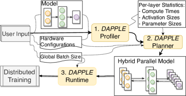
Figure 1: DAPPLE framework overview.

More specifically, the planner aims at minimizing the end-to-end execution time of one training iteration. This module is responsible for stage partition, stage replication and device assignment and generates optimal parallelization plans. In particular, the device assignment process is aware of the hardware topology, as shown in Fig. 1.

TABLE I: The traffic volume.

Benchmark	Activation Size at the Partition Boundaries	Gradient Size
GNMT-16	$26$MB	$1.1$GB
BERT-48	$8.8$MB	$2.8$GB
XLNET-36	$4.2$MB	$2.1$GB
AmoebaNet-36	$11.2$MB	$3.7$GB
VGG-19	$6$MB	$550$MB

We also explore the mapping of a single stage onto multiple devices. With the replication of pipeline stages on multiple devices, DAPPLE processes training with the hybrid of data and pipeline parallelism. In practice, this hybrid strategy can exploit hierarchical interconnects effectively. Fig. 2 gives an example where a model is partitioned into two stages and each stage is replicated on four devices within the same server(NVLink connections within server), while inter-stage communication goes over the Ethernet. This mapping exploits workload characteristics (Table I) by leveraging the high-speed NVLink for heavy gradients sync, while using the slow Ethernet bandwidth for small activations communication. We discuss details of our planner in Section IV.

Finally, the DAPPLE runtime involves a carefully designed scheduling algorithm. Unlike existing pipeline scheduling algorithms [21], DAPPLE scheduler (Section III) significantly reduces the need for re-computation, retains a reasonable level of memory consumption, while saturates the pipeline with enough micro-batches to keep all devices busy.

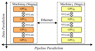
Figure 2: Device mapping on hierarchical interconnects.

III DAPPLE Schedule

III-A Limitations of GPipe Schedule

To improve pipeline training efficiency, GPipe[10] proposes to split global batch into multiple micro-batches and injects them into the pipeline concurrently (Fig. 3 (a)). However, this scheduling pattern alone is not memory-friendly and will not scale well with large batch. The activations produced by forward tasks have to be kept for all micro-batches until corresponding backward tasks start, thus leads to the memory demand to be proportional ($O(M)$) to the number of concurrently scheduled micro-batches ($M$). GPipe adopts re-computation to save memory while brings approximately 20% extra computation. In DAPPLE, we propose early backward scheduling to reduce memory consumptions while achieving good pipeline training efficiency(Fig. 3 (b)).

III-B Early backward scheduling

The main idea is to schedule backward tasks(BW) earlier and hence free the memory used for storing activations produced by corresponding forward tasks(FW). Fig. 3(b) shows DAPPLE’s scheduling mechanism, compared to GPipe in Fig. 3 (a). Firstly, instead of injecting all $M$ micro-batches at once, we propose to inject K micro-batches ($K<M$) at the beginning to release memory pressure while retaining high pipeline efficiency. Secondly, we schedule one FW of a micro-batch followed by one BW strictly to guarantee that BW can be scheduled earlier. Fig. 3 (c) shows how the memory consumptions change over time in GPipe and DAPPLE. At the beginning, the memory usage in DAPPLE increases with time and is the same as GPipe’s until $K$ micro-batches are injected, then it reaches the maximum due to the early BW scheduling. Specifically, with strictly controlling the execution order of FW and BW, the occupied memory for activations produced by the FW of a micro-batch will be freed after the corresponding BW so that it can be reused by the next injected micro-batch. In comparison, GPipe’s peak memory consumptions increases continuously and has no opportunity for early release. Moreover, DAPPLE does not sacrifice in pipeline training efficiency. Actually, DAPPLE introduces the exact same bubble time as GPipe when given the same stage partition, micro-batches and device mapping. We will present the details in section V-C.

Note that the combination of early backward scheduling and re-combination allows further exploitation in memory usage. We present performance comparisons of DAPPLE and GPipe in section VI-D.

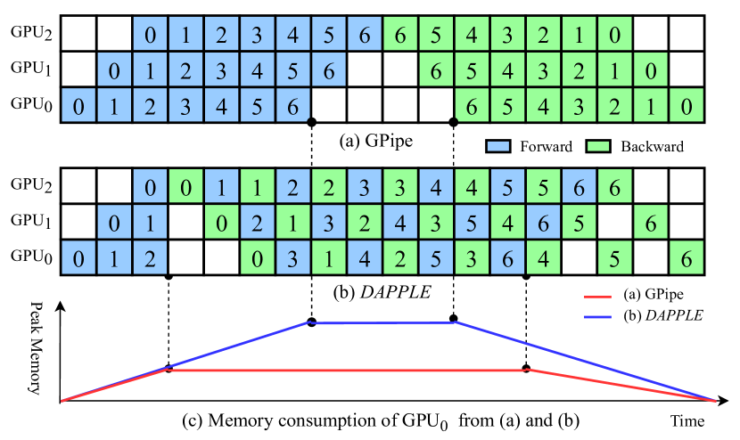
Figure 3: The different scheduling between GPipe(a) and DAPPLE(b) and their memory consumptions.

IV DAPPLE Planner

DAPPLE Planner generates an optimal hybrid parallelism execution plan given profiling results of DAPPLE profiler, hardware configurations and a global training batch size.

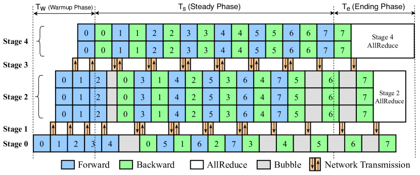
Figure 4: DAPPLE pipeline example.

IV-A The Optimization Objective

For synchronous training, we use the execution time of a single global batch as our performance metric, which we call pipeline latency. The optimization objective is to minimize pipeline latency $L$ with the consideration of all solution spaces of data/pipeline parallelism.

In synchronous pipelined training, computations and cross-stage communication of all stages usually form a trapezoid, but not diamond formed by normal pipelines without backward phase. Fig.4 shows a pipelined training example with well designed task scheduling arrangement. We use blue blocks for forward computation, and green ones for backwards, with numbers in them being the corresponding micro-batch index. Network communications are arranged as individual stages. Gray blocks are bubbles.

We denote the stage with the least bubble overhead as pivot stage, which will be the dominant factor in calculating pipeline latency $L$. Let its stage id be $Q$. We will discuss about how to choose pivot stage later.

A pipeline training iteration consists of warmup phase, steady phase and ending phase, as shown in Fig. 4 in which pivot stage is the last stage. Pivot stage dominates steady phase. We call the execution period from the start to pivot stage’s first micro-batch as warmup phase in a pipeline iteration, the period from pivot stage’s last micro-batch to the end as ending phase. Pipeline latency is the sum of these three phases. The optimization objective for estimating $L$ is as follows:

$$\begin{split}T_{w}&=\sum_{s=0}^{Q}F_{s}\\ T_{s}&=(M-1)\times(F_{Q}+B_{Q})\\ T_{e}&=\max_{s=0}^{S-1}(AR(P_{s},g_{s})+\begin{cases}-\sum_{a=Q}^{s}B_{a}&s\geq Q\\ \sum_{a=s}^{Q}B_{a}&s<Q\end{cases})\\ \end{split}$$ (1)

$$L=T_{w}+T_{s}+T_{e}$$ (2)

$T_{w}$ denotes the execution time of warmup phase, which is the sum of forward execution time of stages till $Q$ for one micro-batch. $T_{s}$ denotes the steady phase, which includes both forward and backward time of stage $Q$ for all micro-batches except for the one contributing to warmup and ending phase. $T_{e}$ corresponds to the ending phase. $T_{e}$ includes allreduce overhead and thus considers stages both before and after $Q$. Note that some stages before $Q$ may contribute to $T_{e}$ with allreduce cost. $M$, $S$, $F_{s}$ and $B_{s}$ denote the total number of micro-batches, the number of stages (computation stages + network stages), forward and backward computation time of stage $s$, respectively. $AR(P_{s},g_{s})$ represents the gradients synchronization (AllReduce) time for stage $s$, with its parameter set $P_{s}$ on the device set $g_{s}$.

Note we consider inter-stage communication as an independent stage alongside the computation stages. The AllReduce time $AR(P_{s},g_{s})$ is always 0 for communication stages. Moreover, we define $F_{s}$ and $B_{s}$ for a communication stages as its following forward and backward communication time.

In practice, synchronous pipelines in some cases include bubbles in stage $Q$, which may contribute a small fraction of additional delay to time. This objective does not model those internal bubbles, and thus is an approximation to the true pipeline latency. But it works practically very well for all our benchmarks (Section VI).

IV-B Device Assignment

Device assignment affects communication efficiency and computing resource utilization. Previous work [12] uses hierarchical planning and works well for asynchronous training. However, it lacks consideration of synchronous pipeline training, in which the latency of the whole pipeline, rather than of a single stage, matters to overall performance. It cannot be used to efficiently estimate the whole pipeline latency. Meanwhile, it does not allow stages to be placed on arbitrary devices. Our approach essentially allows a specific stage to be mapped to any set of devices, and therefore is able to handle more placement cases, at a reasonable searching cost.

Instead of enumerating all possibilities of placement plans using brute force, we designed three policies (Fig. 5), and explore their compositions to form the final placement plan.

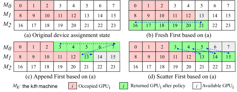
Figure 5: Device assignment examples: applying for $6$ devices using three different strategies respectively from (a).

Fresh First

allocate GPUs from a fresh machine. It tends to put tasks within a stage onto the same machine, which can leverage high-speed NVLink [22] for intra-stage communication. A problem of this policy is that, it can cause fragmentation if the stage cannot fully occupy the machine.

Append First

allocate from machines that already have GPUs occupied. It helps to reduce fragmentation. It also largely implies that the stage is likely to be within the same machine.

Scatter First

try to use available GPUs equally from all used machines, or use GPUs equally from all machines if they are all fresh. It is suitable for those stages that have negligible weights compared to activation sizes (less intra-stage communication). This policy could also serve as an intermediate state to allocate GPU with minimal fragmentation.

The overall device placement policies reduce search space effectively down to less than $O(2^{S})$, while retaining room for potential performance gain.

IV-C Planning Algorithm

Our planning algorithm use Dynamic Programming to find the optimal partition, replication and placement strategy, so that the pipeline latency $L$ is minimized. Here we first present how to update the pivot stage ID $Q$ along the planning process, and then the formulation of our algorithm

IV-C1 Determining The Pivot Stage $Q$

It is vital to select a proper pivot stage $Q$ for the estimation of $L$. The insight is to find the stage with minimum bubbles, which dominates steady phase. We use a heuristic to determine $Q$ (formula 3).

$$\begin{split}Q&=\arg\max_{s=S-1}^{0}\max\Big{(}T_{st}^{Q}+\sum_{s^{\prime}=s+1}^{Q-1}(F_{s^{\prime}}+B_{s^{\prime}}),T_{st}^{s}\Big{)}\end{split}$$ (3)

The initial $Q$ is set to $S-1$. DAPPLE updates $Q$ iteratively from stage $S-1$ to stage $0$ according to formula 3. $T_{st}^{j}=(M-1)\times(F_{j}+B_{j})$ means the duration of steady phase, without bubbles, suppose pivot stage is $j$. For a stage $s<Q$, if $T_{st}^{s}$ is larger than the sum of $T_{st}^{Q}$ and corresponding forward/backward costs between $s$ and current $Q$, it means the steady phase will have less bubbles if pivot stage is set as $s$ other than current $Q$. $Q$ will then be updated to $s$.

IV-C2 Algorithm Formulation

We define the estimated pipeline latency $T_{PL}(j,m,g)$ as the subproblem, for which we have planned the strategy for the first $j$ layers using $m$ GPUs (with device id set $g$). The unplanned layers forms the last stage and replicates on the other $(G-m)$ GPUs. Our objective is to solve for $T_{PL}(N,G,\mathcal{G}),\mathcal{G}=\{0,1,...,G-1\}$. $N$, $G$ and $\mathcal{G}$ denote the number of layers, number of GPUs and GPU set, respectively. Formula 4 describes the algorithm.

$$\left.T_{PL}(N,G,\mathcal{G})\right.=\min_{1\leq j<N}\min_{1\leq m<G}\min_{g\in D(\mathcal{G},m)}\left.T_{PL}(j,m,g)\right.$$ (4)

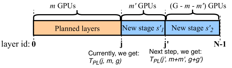
Figure 6: Planning process for j’.

Fig. 6 describes the iterative planning process. Suppose we have already planned for the first $j$ ($0\leq j<N$) layers and have the estimation $T_{PL}(j,m,g)$ as pipeline latency. The layers after $j$ forms a stage $s^{\prime}$. Meanwhile, we get the optimal $Q$ for current strategy along with the cost of $F_{Q}$ and $B_{Q}$ for stage $Q$. Next step, we try to add one more partition in stage $s^{\prime}$, supposing after layer $j^{\prime}$ ($j<j^{\prime}\leq N$), and split $s^{\prime}$ into two new stages $s^{\prime}_{1}$ and $s^{\prime}_{2}$. We assign $m^{\prime}$ GPUs for $s^{\prime}_{1}$ and $(G-m-m^{\prime})$ GPUs for $s^{\prime}_{2}$, and estimate $T_{PL}(j^{\prime},m+m^{\prime},g+g^{\prime})$ according to formula 5. Note DAPPLE enumerates the three strategies in section IV-B for device placement of stage $s^{\prime}_{1}$.

$$\begin{split}T_{PL}(j^{\prime},m+m^{\prime},g+g^{\prime})=L&\end{split}$$ (5)

Here, $L$ is the same with that in formula 2. The key for the estimation of $L$ in formula 5 is to find $Q$ of subproblem $T_{PL}(j^{\prime},m+m^{\prime},g+g^{\prime})$. In the sample in Fig. 6, we get $Q_{j}$ for $T_{PL}(j,m,g)$. We apply formula 3 to get $Q_{j^{\prime}}$ for $T_{PL}(j,m+m^{\prime},g+g^{\prime})$ with the help of $Q_{j}$: if $Q_{j}$ is not $s^{\prime}$, we do not need to iterate all stages before $j$, but use $Q_{j}$ for all stages before layer $j$ instead in the iterative process.

Along the above process, we record the current best split, replication and placement for each point in our solution space using memorized search.

IV-D Contributions over previous work

Previous works on pipeline planning includes PipeDream[12] (for asynchronous training) and torchgpipe[23], a community implementation of GPipe[10] which uses “Block Partitioning of Sequences” [24]. Both aim to balance the workload across all GPUs. While this idea works good in PipeDream’s asynchronous scenarios and gives reasonable solutions under GPipe’s synchronous pipeline for its micro-batch arrangement, we found that our micro-batch arrangement could achieve even higher performance by 1) intentionally preferring slightly uneven partitioning with fewer stages, and 2) exploring a broader solution space of device assignment. The following sections highlight our contributions of planning for hybrid parallelism. The resulting strategies and performance gain on real-world models will be demonstrated in Section VI-F.

IV-D1 Uneven Pipeline Partitioning with Fewer Stages

In synchronous Pipeline Parallelism scenarios, we found two insights that could provide an additional performance improvements. The first one is to partition the model into as few stages as possible to minimize the bubble overhead under the same number of micro-batches. This conclusion is also mentioned in GPipe. The second one is that partitioning the model in a slightly uneven way yields much higher performance than a perfectly even split, like the example in Fig. 7.

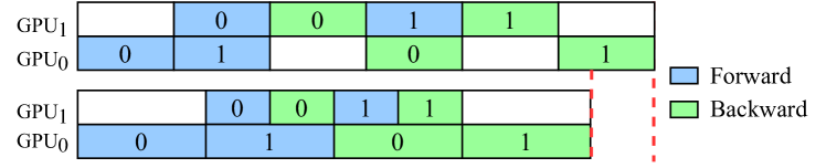
Figure 7: Uneven pipeline minimum example.

IV-D2 Versatile Device Placement

DAPPLE device assignment strategy covers a broad solution space for stage placement, and is a strict superset of PipeDream’s hierarchical recursive partitioning approach. This allows us to handle various real world models. For example, for models that have layers with huge activations compared to their weights, DAPPLE allows such a layer to be replicated across multiple machines (Scatter First) to utilize high-speed NVLink for activation communication and low-speed Ethernet for AllReduce.

V DAPPLE Runtime

V-A Overview

We design and implement DAPPLE runtime in Tensorflow[25] (TF) 1.12, which employs a graph based execution paradigm. As common practices, TF takes a precise and complete computation graph (DAG), schedules and executes graph nodes respecting all data/control dependencies.

DAPPLE runtime takes a user model and its planning results as input, transforms the model graph into a pipelined parallel graph and executes on multiple distributed devices. It first builds forward/backward graphs separately for each pipe stage. Then additional split/concat nodes are introduced between adjacent stages for activation communication. Finally, it builds a subgraph to perform weights update for synchronous training. This step is replication aware, meaning it will generate different graphs with or without device replication of stages. We leverage control dependences in TF to enforce extra execution orders among forward/backward stage computations. Section V-B presents how to build basic TF graph units for a single micro-batch. Section V-C discusses how to chain multiple such units using control dependencies to facilitate DAPPLE execution.

V-B Building Micro-batch Units

V-B1 Forward/Backward Stages

In order to enforce execution orders with control dependencies between stages, we need to build forward and backward graphs stage by stage to deal with the boundary output tensors such as activations.

Specifically, we first construct the forward graph of each stage in sequence and record the boundary tensors. No backward graphs should be built until all forward graphs are ready. Second, backward graphs will be built in reverse order for each stage.

V-B2 Cross Stage Communication

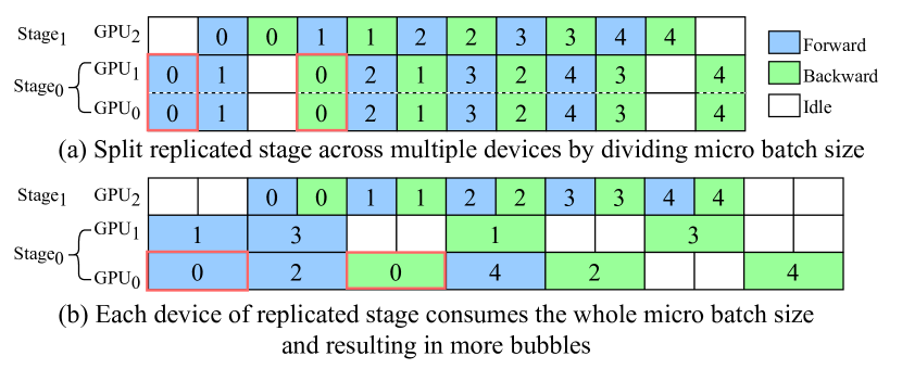
Figure 8: Efficiency of two stage replication approaches. Stage 0 consumes twice as much time as stage 1 for a micro-batch.

DAPPLE replicates some stages such that the number of nodes running a stage can be different between adjacent stages, and the communication patterns between them are different from straight pipeline design. We introduce special split-concat operations between these stages.

Fig. 8(a) shows the replication in DAPPLE for a 2-stage pipeline, whose first stage consumes twice as much time as the second stage for a micro-batch and thus is replicated on two devices. For the first stage, we split the micro-batch further into 2 even slices, and assign each to a device. An alternative approach[12] (Fig. 8(b)) is not to split, but to schedule an entire micro-batch to two devices in round robin manner. However, the second approach has lower pipeline efficiency due to tail effect[26]. Though the second approach does not involve extra split-concat operations, the overhead of tail effect is larger than split-concat in practice. We hence use the first approach with large enough micro-batch size setting to ensure device efficiency.

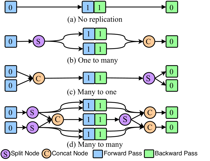
Figure 9: Split-Concat for Cross Stage Communication

The split-concat operations include one-to-many, many-to-one and many-to-many communication. We need split for one-to-many(Fig. 9(b)), that is, splitting the micro-batch into even slices and sending each slice to a device in the next stage. We need concat for many-to-one(Fig. 9(c)), where all slices should be concatenated from the previous stage and fed into the device in the next stage. For many-to-many(Fig. 9(d)) we need both split and concat of micro-batch slices to connect adjacent stages. If two adjacent stages have the same replication count, no split-concat is needed.

V-B3 Synchronous Weights Update

Weights updating in DAPPLE is different with naive training as there are multiple micro-batches injected concurrently. Meanwhile, the replication makes weights updating more complex. As is shown in Fig. 10, each device produces and accumulates gradients for all micro-batches. There is an AllReduce operation to synchronize gradients among all replicas, if exists. A normal Apply operation updates weights with averaged gradients eventually.

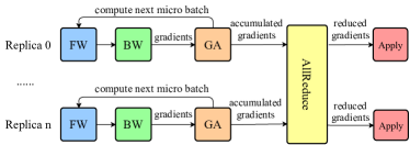
Figure 10: Weights update. GA means gradient accumulation[5].

V-C Micro-batch Unit Scheduling

The early backward scheduling strikes a trade-off between micro-batch level parallelism and peak memory consumption: feeding more micro-batches into pipeline at once implies higher parallelism, but may lead to more memory usage.

DAPPLE scheduler enforces special execution orders between micro-batches to reduce memory usage. For the first stage, we suppose $K$ micro-batches are scheduled concurrently at the beginning for forward computation. Specifically, $K_{i}$ is the number of scheduled micro-batches at the beginning for stage $i$. The overall execution follows a round robin order with interleaving FW and BW.

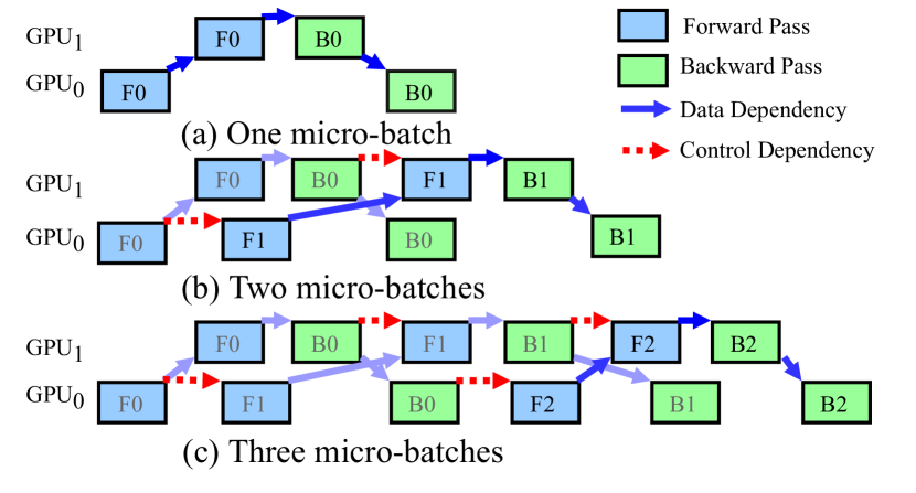
Figure 11: Micro-batches scheduling. The solid blue and dotted red arrows denote data and control dependencies, respectively.

We realize the scheduler with control dependency edges in TF. Fig. 11 shows how up to three micro-batches are connected via control dependencies to implement the schedule for a two stage pipeline. Control dependency is not necessary when there is only one micro-batch (Fig. 11(a)). With two micro-batches (Fig. 11(b)), two control edges are introduced. The control edge between $B0$ and $F1$ in stage $1$ is to form the round robin order of FW and BW. The early execution of $B0$ helps to free memory of $F0$ and $B0$ in stage 1, which can be reused in following tasks. The edge between $F0$ and $F1$ in stage $0$ is to enforce the order that micro-batch 1 is strictly executed after micro-batch 0, thus the backward of micro-batch 0 can be executed earlier and its corresponding memory can be freed earlier. In practice, $F0$ and $F1$ are typically large chunks of computations. The lack of parallelism between $F0$ and $F1$ does not affect the gain of reducing memory usage. The situation with three micro-batches (Fig. 11(c)) is the same.

An appropriate $K_{i}$ is essential as it indicates the peak memory consumption for stage $i$. There are two primary factors for deciding $K_{i}$: memory demand for one micro-batch execution, and the ratio between cross stage communication latency and the average FW/BW computation time (referred as activation communication ratio, ACR in short). The former determines how many forward batches can be scheduled concurrently at most. We define the maximum number of micro-batches supported by the device memory as $D$; Lower ACR means less warm up forward batches $K_{i}$ (smaller $K_{i}$) are enough to saturate the pipeline. While notable ACR means larger $K_{i}$ is necessary.

We implement two policies to set $K_{i}$ in practice. Policy A ($P_{A}$): $K_{i}=min(S-i,D)$. $P_{A}$ works well when ACR is small, i.e. the impact of cross stage communication overhead is negligible. Policy B ($P_{B}$): $K_{i}=min(2*(S-i)-1,D)$. Here we schedule twice the number of forward micro-batches than $P_{A}$. The underlying intuition is that in some workloads, the cross stage communication overhead is comparable with forward/backward computations and thus more micro-batches is needed to saturate the pipeline.

VI Evaluation

VI-A Experimental Setup

Benchmarks. Table II summarizes all the six representative DNN models that we use as benchmarks in this section. The datasets applied for the three tasks are WMT16 En-De [27], SQuAD2.0 [28] and ImageNet[29], respectively.

TABLE II: Benchmark models.

Task	Model	# of Params	(cbch Size, Memory Cost)
Translation	GNMT-16 [30]	291M	(64, 3.9GB)
Language Model	BERT-48 [31]	640M	(2, 11.4GB)
	XLNet-36 [32]	500M	(1, 12GB)
Image Classification	ResNet-50 [33]	24.5M	(128, 1GB)
	VGG-19 [34]	137M	(32, 5.6GB)
	AmoebaNet-36 [35]	933M	(1, 20GB)

TABLE III: Hardware configurations.

Config	GPU(s) per server($N_{s}$)	Intra-server connnections	Inter-server connections
A	8x V100	NVLink	25 Gbps
B	1x V100	N/A	25 Gbps
C	1x V100	N/A	10 Gbps

Hardware Configurations. Table III summarizes three common hardware environments for DNN training in our experiments, where hierarchical and flat interconnections are both covered. In general, hierarchical interconnection is popular in industry GPU data centers. We also consider flat Ethernet networks interconnections because NVLink may not be available and GPU resources are highly fragmented in some real-world production clusters. Specifically, Config-A (hierarchical) has servers each with 8 V100 interconnected with NVLink, and a 25Gbps Ethernet interface. Config-B (flat) has servers each with only one V100 (no NVLink) and a 25Gbps Ethernet interface. Config-C (flat) is the same with Config-B except with only 10 Gbps Ethernet equipped. The V100 GPU has 16 GB of device memory. All servers run 64-bits CentOS 7.2 with CUDA 9.0, cuDNN v7.3 and NCCL 2.4.2[36].

Batch Size and Training Setup. The batch sizes of offline profiling for the benchmarks are shown in the last column of Table II (ch size. As for AmoebaNet-36, it reaches OOM even if $batch\_size=1$ on a single V100. Thus we extend to two V100s where $batch\_size=1$ just works. We use large enough global batch size for each benchmark to ensure high utilization on each device. All global batch sizes we use are consistent with common practices of the ML community. We train GNMT-16, BERT-48 and XLNet-36 using the Adam optimizer [37] with initial learning rate of 0.0001, 0.0001, 0.01 and 0.00003 respectively. For VGG19, we use SGD with an initial learning rate of 0.1. For AmoebaNet, we use RMSProp [38] optimizer with an initial learning rate of 2.56. We use fp32 for training in all our experiments. Note that all the pipeline latency optimizations proposed in this paper give equivalent gradients for training when keeping global batch size fixed and thus convergence is safely preserved.

VI-B Planning Results

TABLE IV: Normalized training throughput speedup of scheduling policies $P_{B}$ compared to $P_{A}$.

Model	Bert-48	XLNet-36	VGG-19	GNMT-16
Speedup	1.0	1.02	1.1	1.31

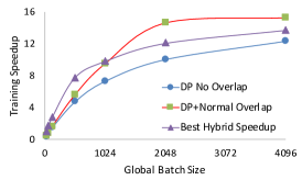
(a) VGG19 on config $A$

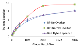
(b) VGG19 on config $B$

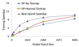
(c) VGG19 on config $C$

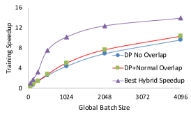
(d) GNMT-16 on config $A$

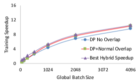
(e) GNMT-16 on config $B$

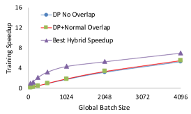
(f) GNMT-16 on config $C$

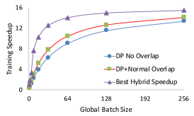
(g) BERT-48 on config $A$

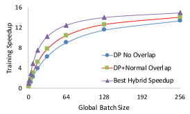
(h) BERT-48 on config $B$

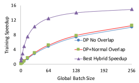
(i) BERT-48 on config $C$

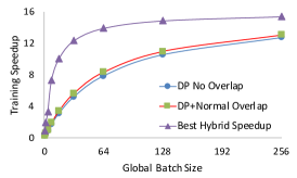
(j) XLNet-36 on config $A$

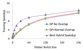
(k) XLNet-36 on config $B$

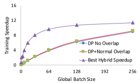
(l) XLNet-36 on config $C$

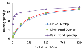
(m) AmoebaNet-36 on config $A$

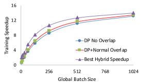
(n) AmoebaNet-36 on config $B$

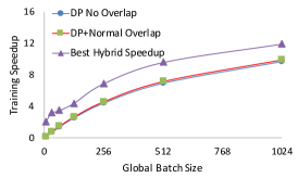
(o) AmoebaNet-36 on config $C$

Figure 12: Speedups on configurations with hierarchical/flat interconnects.

TABLE V: DAPPLE planning results.

Model (GBS)	$\#Servers\times N_{s}$	Output Plan	Split Position	$ACR$
ResNet-50 (2048)	$2\times 8$ (A)	DP	-	-
	$16\times 1$ (B)	DP	-	-
	$16\times 1$ (C)	DP	-	-
VGG-19 (2048)	$2\times 8$ (A)	DP	-	-
	$16\times 1$ (B)	DP	-	-
	$16\times 1$ (C)	$15:1$	$13:6$	0.40
GNMT-16 (1024)	$2\times 8$ (A)	$8:8$	$9:7$	0.10
	$16\times 1$ (B)	$8:8$	$9:7$	0.10
	$16\times 1$ (C)	Straight	-	3.75
BERT-48 (64)	$2\times 8$ (A)	$8:8$	$23:25$	0.06
	$16\times 1$ (B)	Straight	-	0.50
	$16\times 1$ (C)	Straight	-	1.25
XLNet-36 (128)	$2\times 8$ (A)	$8:8$	$18:18$	0.03
	$16\times 1$ (B)	$8:8$	$18:18$	0.03
	$16\times 1$ (C)	Straight	-	0.67
AmoebaNet-36 (128)	$2\times 8$ (A)	$8:8$	$24:12$	0.18
	$16\times 1$ (B)	$11:5$	$27:9$	0.14
	$16\times 1$ (C)	$11:5$	$27:9$	0.35

Table V summarizes DAPPLE planning results of five models in the three hardware environments, where the total number of available devices are all fixed at $16$. The first column also gives the global batch size ($GBS$) correspondingly.

We use three notations to explain the output plans. (1) A plan of $P:Q$ indicates a two stage pipeline, with the first stage and the second stages replicated on $P$ and $Q$ devices, respectively. For example, when $P=8$ and $Q=8$, we put each stage on one server, and replicate each stage on all 8 devices within the server(config-A). Besides, for plans where $P>8$ or $Q>8$ (e.g., $15:1$) where some stages are replicated across servers, it will most likely be chosen for configurations with flat interconnections such as Config-B or Config-C, since for Config-A replicating one stage across servers incurs additional inter-server communication overhead. (2) A straight plan denotes pipelines with no replication. (3) A DP plan means the optimal strategy is data-parallel. We treat DP and straight as special cases of general DAPPLE plans.

The Split Position column of Table V shows the stage partition point of each model for the corresponding pipeline plan. The $ACR$ column of the table shows the $averaged$ ratio of cross-stage communication latency (i.e. communication of both activations in FW and gradients in BW) and stage computation time.

In the case of single server of config $A$, there is no relative low-speed inter-server connection, the intra-server bandwidth is fast enough (up to $130GB/s$) to easily handle the magnitude (up to $3.7GB$) of gradients communication of all benchmark models, and we find all models prefer DP plan for this case.

ResNet-50. The best plan is consistently DP for all three hardware configurations. This is not surprising due to its relatively small model size (100MB) yet large computation density. Even with low speed interconnects config $C$, DP with notably gradients accumulation and computation/communication overlap outperforms the pipelined approach.

VGG-19. Best plans in config $A$ and $B$ are also DP (Fig. 12 (a) and(b)), due to the moderate model size (548MB), relatively fast interconnects (25 Gbps), and the overlapping in DP. The weights and computation distributions of VGG19 are also considered overlapping-friendly, since most of the weights are towards the end of the model while computations are at the beginning, allowing gradients aggregation to be overlapped during that computation-heavy phase. In the case of low speed interconnects (config $C$), a $15:1$ pipelined outperforms DP (Fig. 12 (c). This is because most parameters in VGG-19 agglomerate in the last fully connected layer. A $15:1$ two-stage pipeline thus avoids most of the overheads of gradients synchronization due to replication (note we do not replicate the second stage). In this case gradients synchronization overheads outweigh benefits of DP with overlap.

GNMT-16/BERT-48/XLNet-36. All three models have uniform layer structures, i.e., each layer has roughly the same scale of computations and parameters. And the parameter scales of these models vary from 1.2 GB up to 2.6 GB(Table II). In config-A where all three models achieve low $ACR$ values (0.10, 0.06 and 0.03, respectively, as shown in Table V), a two stage $8:8$ pipeline works best. Unlike VGG-19, the three models’ layers are relatively uniformly distributed, thus a symmetric, evenly partitioning is more efficient. In config $C$, a straight pipeline works best for all three models. In this config, all devices have approximately the same workload. More importantly, no replication eliminates gradients sync overheads for relatively large models (1.2-2.6 GB) on a slow network (10 Gbps). The three models behave differently in config $B$. BERT-48 prefers straight pipeline in config $B$, while GNMT-16 and XLNet-36 keep the same plan results as shown in config $A$. This is because for fixed $16$ devices, $16$ and $48$ uniform layers are more friendly for even partition compared to $36$ layers for flat interconnections.

AmoebaNet-36. For AmoebaNet-36, DP is not available due to device memory limit. AmoebaNet-36 has more complex network patterns than other models we evaluated, and larger ACR in config $A$ as well. Thus, more successive forward micro-batches are needed to saturate the pipeline. For all three configs, two-stage pipeline ($8:8$, $11:5$ and $11:5$, respectively) works best.

VI-C Performance Analysis

In this work, we measure training speed-up as the ratio between the time executing all micro-batches sequentially on a single device and the time executing all micro-batches in parallel by all devices, with the same global batch size.

Fig. 12 shows training speed-ups for all models except ResNet-50 on config A, B and C. For ResNet-50, the planning results are obvious and we simply present it in Table V. For the other models, we compare training speed-ups of three different implementations: (1) Best Hybrid Speedup, performance of the best hybrid plan of pipeline and data parallelism returned by DAPPLE planner; (2) DP No Overlap, performance of DP with gradients accumulation but without computation/communication overlap; (3) DP Overlap, performance of DP with both gradients accumulation and intra-iteration computation/communication overlap between backward computation and gradients communication[20].

Overall analysis across these five models from Fig. 12, for fixed $GBS=128$, we can find that the hybrid approaches from DAPPLE outperform the DP approach with best intra-batch overlapping with averaged 1.71X/1.37/1.79X speedup for config-A, config-B and config-C, respectively. Specially, this speedup is up to 2.32X for GNMT-16 on config-C. Specific analysis for each model is given below.

VGG-19. For VGG-19, about 70% of model weights (about 400 MB) are in the last fully connected (fc) layer, while the activation size between any two adjacent layers gradually decreases from the first convolution layer to the last fc layer, varying dramatically from 384 MB to 3 MB for batch size 32. Thus, the split between VGG-19’s convolutional layers and fully-connected layers leads to very small activation (3MB), and only replicating all the convolutional layers other than fully-connected layers greatly reduces communication overhead in case of relatively slow interconnects (Fig. 12 (c)).

GNMT-16. GNMT-16 prefers a two-stage pipeline on hierarchical network (config $A$) and flat network with relative high-speed connection (config $B$). And the corresponding spit position is $9:7$ but not $8:8$, this is because the per-layer workloads of encoder layer and decoder of GNMT are unbalanced (approximately $1:1.45$), thus the split position of DAPPLE plan shifts one layer up into decoder for pursuit of better system load-balance. For low speed interconnection environments (config $C$), straight pipeline ranks first when $GBS=1024$. Each device is assigned exactly one LSTM layers of GNMT, and the $GBS$ is large enough to fill the 16-stage pipeline.

BERT-48/XLNet-36. The best DAPPLE plan outperforms all DP variants for both models (Fig. 12 (g) to (l)) in all configurations. Compared to XLNet, the memory requirement for BERT is much smaller and thus allows more micro-batches on a single device. More computation per-step implies more backward computation time can be leveraged for overlapping communication overhead. As for config $B$ and $C$, the slower the network is(from 25 Gbps to 10 Gbps), the higher the advantage of our approach has over DP variants. This is because the cross stage communication for both models is negligible with respect to gradients communication and the pipelined approach is more tolerant of slow network than DP.

AmoebaNet-36. The DAPPLE plan works best in all three configurations when GBS is fixed to $128$. Unlike BERT-48 and XLNet-36, AmoebaNet has non uniform distributions of per layer parameters and computation density. The last third part of the model holds 73% of all parameters, and the per-layer computation time gradually increases for large layer id and the overall maximum increase is within 40%. As DAPPLE planner seeks for load-balanced staging scheme while considering the allreduce overhead across replicated stages, the split positions of pipelined approach for AmoebaNet-36 will obviously tilt to larger layer ID for better system efficiency. Take config $A$ as an example, a two-stage pipeline is chosen and each stage is replicated over a separate server with $8$ devices each. For this case a total of $36$ normal cells layers are divided into $2$ parts, namely $24:12$, where the per-stage computation time ratio and allreduce time ratio of $stage_{0}$ and $stage_{1}$ is $1.57:1$ and $1:2.74$, respectively. For lower bandwidth network configurations (config $B$ and $C$), the split position keeps shrinking to larger layer ID, because the allreduce comm overheads turn out to be the dominant factor with the absent of high-speed NVLink bandwidth.

VI-D Scheduling Policy

As discussed in Section V-C, the number of successive forward micro-batches ($K_{i}$ for stage $i$) scheduled in the warm up phase is an important factor to pipeline efficiency. We implement two policies, $P_{A}$ and $P_{B}$, referring to smaller and larger $K_{i}$ numbers, respectively. Table IV shows the normalized speedups for four benchmark models on hierarchical interconnects(config $A$), where all models’ stage partition and replication schemes are consistent with the planning results of 2 servers of config $A$ as shown in Table V.

For VGG-19 and GNMT-16 (as well as AmoebaNet-36, which is not given in this figure yet), where the $ACR$ ratio is relative high (0.16, 0.10, 0.18, respectively), there exists notable performance difference between these two policies (10%, 31% improvement from $P_{A}$ to $P_{B}$, respectively). Hence we choose a larger $K_{i}$ to maximize pipeline efficiency. For the other models (BERT-48, XLNet-36), whose $ACRs$ are very small (0.06, 0.03, respectively), the cross stage communication overhead is negligible compared to intra-stage computation time, leading to little performance difference. In this case, we prefer a smaller $K_{i}$ to conserve memory consumption.

TABLE VI: DAPPLE vs. GPipe on BERT-48 with $2$-stage pipeline when keeping micro-batch size fixed to $2$ on Config-B. RC is short for re-computation.

Config	# of micro batch ($M$)	Throughput (samples/sec)	Average Peak Memory (GB)
GPipe	2	5.10	12.1
	3	–	$OOM$
GPipe + RC	2	4.00	9.9
	5	5.53	13.2
	8	–	$OOM$
DAPPLE	2	5.10	10.6
	8	7.60	10.6
	16	8.18	10.6
DAPPLE + RC	2	4.24	8.5
	8	6.23	8.5
	16	6.77	8.5

VI-E Comparison with GPipe

Table VI shows the performance comparisons with GPipe. We focus on the throughput and peak memory usage on BERT-48 with a 2-stage pipeline on Config-B. To align with GPipe, we adopt the same re-computation strategy which stores activations only at the partition boundaries during forward. Note that all the pipeline latency optimizations in DAPPLE give equivalent gradients for training when keeping global batch size fixed and thus convergence is safely preserved and will not be further analysed here.

When applying re-computation, both DAPPLE and GPipe save about 19% averaged peak memory at the expense of 20% on throughput when keeping $M=2$ fixed.

When both without re-computation, DAPPLE gets $1.6\times$ higher throughput with $M=16$, and consumes $0.88\times$ averaged peak memory compared to GPipe, which only supports up to 2 micro-batches. The speedup is mainly because higher $M$ leads to lower proportion of $bubbles$. Note DAPPLE allows more micro-batches as the peak memory requirement is independent of $M$ due to early backward scheduling.

The combination of DAPPLE scheduler and re-computation allows a further exploitation in memory usage. Compared with baseline GPipe (without re-computation), DAPPLE + RC achieves $0.70\times$ memory consumption when $M=16$, which allows us to handle larger micro-batch size or larger model.

VI-F Comparison with PipeDream

TABLE VII: Strategy Comparison between DAPPLE and PipeDream, in the form of (start layer, end layer)@[GPU IDs].

Model (GBS)	DAPPLE	PipeDream
VGG19 (1024)	(0, 16) @ [G0 - G13] (17, 25) @ [G14, G15]	(0, 11) @ [G0 - G7] (11, 17) @ [G8 - G13] (17, 19) @ G14 (19, 25) @ G15
AmoebaNet-36 (128)	(0, 30) @ [G0 - G7] (31, 43) @ [G8 - G15]	straight
BERT Large (128)	(0, 13) @ [G0 - G7] (14, 26) @ [G8 - G15]	(0, 4) @ [G0, G1] (4, 13) @ [G2 - G7] (13, 16) @ [G8, G9] (16, 19) @ [G10, G11] (19, 22) @ [G12, G13] (22, 26) @ [G14, G15]
XLNet-36 (128)	(0, 22) @ [G0 - G7] (23, 41) @ [G8 - G15]	straight

We compare the results of our planner with those of PipeDream’s under the synchronous training scenarios. We use the same configurations for both planners (e.g. same device topology, same interconnect and same profiling data), and evaluate both planners with DAPPLE Runtime. Table VII shows the strategy results under a two-machine cluster of config-A. Fig. 13 shows the performance results for the strategies running in both $2\times 8$ and $4\times 8$ configurations.

As shown in Fig. 13, in terms of $speedup$ relative to to data parallelism, our strategies consistently outperform those generated by PipeDream’s planner by up to $3.23\times$ speedup under synchronous training scenarios, thanks to the advantages detailed in Section IV-D.

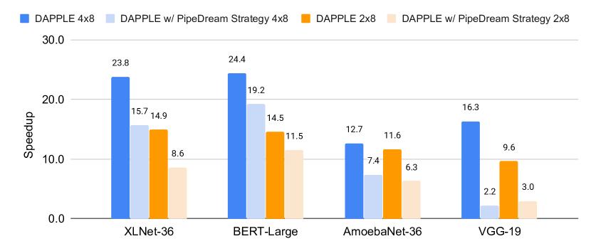
Figure 13: Performance comparison with PipeDream.

VI-G Strong Scaling

Fig. 14 shows training speed-ups for four models. The number of GPUs ranges from 2 to 16. We use fixed but different global batch size for each model and apply config $A$. For AmoebaNet-36 when $GBS=256$ (Fig. 14(d)), both DP approaches achieve NaN as the model size is too large to fit memory of single V100. For all these four models, we observe better scalability of DAPPLE over DP variants. Scalability weakens on all DP variants when the number of GPUs increases from 8 to 10, where gradients synchronization performance drops substantially due to slow Ethernet bandwidth. The performance of $DAPPLE$ approach scales smoothly due to the rather small magnitude of cross-stage activations as compared with weights(Table I), which is insensitive to the relatively low-speed inter-server communications(25Gbps). In general, for hierarchical interconnects, the lower the cross-machine bandwidth, the more obvious the advantage $DAPPLE$ approach as compared with $DP$.

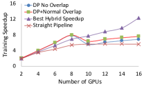
(a) GNMT-16($GBS=2048$)

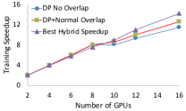
(b) BERT-48($GBS=128$)

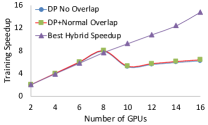
(c) XLNet-36($GBS=128$)

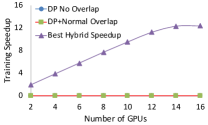
(d) AmoebaNet-36($GBS=256$)

Figure 14: Speedup with fixed $GBS$ in config-A.

VI-H Weak Scaling

Table VIII shows the maximum model size that DAPPLE supports under reasonable input size with re-computation. We scale the model by varying the numbers of layers. We are able to scale BERT to 5.5B on 8 V100s with NVLink. There is a slight reduction in average GPU utilization due to more bubbles introduced by longer pipeline. In this case, the maximum model size scales linearly due to the balanced distribution of model params over encoder layers in BERT.

TABLE VIII: Maximum model size of BERT supported by DAPPLE + re-computation on V100 (16GB each) on config-A. BERT-L: BERT model with $L$ encoder layers. Each model parameter needs 16 bytes since we applied Adam optimizer.

Config	BERT-L	# of Model Params	Total Model Params Mem	Avg. GPU Util
Native-1	48	640M	10.2GB	93%
Pipeline-2	106	1.4B	21.9GB	89%
Pipeline-4	215	2.7B	43.8GB	89%
Pipeline-8	428	5.5B	88.2GB	87%

VII Related Work

Large DNN models are increasingly computational intensive. It is a common practice to parallelize training by leveraging multiple GPUs[39, 40, 41, 42]. Data parallelism, model parallelism and pipeline parallelism are common approaches for distributed training of DNN models.

Data Parallelism[43] . Some prior studies [44, 45, 46, 47, 9, 48] focus on reducing the communication overheads for data parallelism. As a commonly used performance optimization method, gradients accumulation[49, 6, 5] offers an effective approach to reduce communication-to-computation ratio. Another complementary approach is computation and communication overlap, with promising results reported in some CNN benchmarks[20, 8].

Model Parallelism. Model Parallelism[50] partitions DNN models among GPUs to mitigate communication overhead and memory bottlenecks for distributed training [51, 40, 39, 52, 14, 10, 53, 54]. This paper focuses on model partition between layers, namely, pipeline parallelism.

Pipeline parallelism. Pipeline Parallelism[14, 11, 10, 55, 21] has been recently proposed to train DNN in a pipelined manner. GPipe[10] explores synchronous pipeline approach to train large models with limited GPU memory. PipeDream[14] explores the hybrid approach of data and pipeline parallelism for asynchronous training. [56, 55, 53] make further optimization based on PipeDream. Pal et al. [40] evaluated the hybrid approach without thorough study. Some researchers have been seeking for the optimal placement strategy to assign operations in a DNN to different devices[57, 58, 59] to further improve system efficiency.

VIII Conclusion

In this paper, we propose DAPPLE framework for pipelined training of large DNN models. DAPPLE addresses the need for synchronous pipelined training and advances current state-of-the-art by novel pipeline planning and micro-batch scheduling approaches. On one hand, DAPPLE planner module determines an optimal parallelization strategy given model structure and hardware configurations. It considers pipeline partition, replication and placement, and generates a high-performance hybrid data/pipeline parallel strategy. On the other hand, DAPPLE scheduler module is capable of simultaneously achieving optimal training efficiency and moderate memory consumption, without storing multiple versions of parameters and getting rid of the strong demand of re-computation which hurts system efficiency at the same time. Experiments show that DAPPLE planner consistently outperforms strategies generated by PipeDream‘s planner by up to $3.23\times$ speedup under synchronous training scenarios, and DAPPLE scheduler outperforms GPipe by $1.6\times$ speedup of training throughput and saves 12% of memory consumption at the same time.

References

- [1] R. Sutton, The Bitter Lesson, 2019, http://www.incompleteideas.net/IncIdeas/BitterLesson.html.
- [2] C. Raffel, N. Shazeer, A. Roberts, K. Lee, S. Narang, M. Matena, Y. Zhou, W. Li, and J. P. Liu, “Exploring the limits of transfer learning with a unified text-to-text transformer,” https://arxiv.org/abs/1910.10683, 2019.
- [3] J. Wang, P. Huang, H. Zhao, Z. Zhang, B. Zhao, and D. L. Lee, “Billion-scale commodity embedding for e-commerce recommendation in alibaba,” in Proceedings of the 24th ACM SIGKDD International Conference on Knowledge Discovery and Data Mining. ACM, 2018, pp. 839–848.
- [4] P. Covington, J. Adams, and E. Sargin, “Deep neural networks for youtube recommendations,” in Proceedings of the 10th ACM Conference on Recommender Systems, ACM, New York, NY, USA. ACM, 2016.
- [5] Gradients Accumulation-Tensorflow, 2019, https://github.com/tensorflow/tensorflow/pull/32576.
- [6] Gradients Accumulation-PyTorch, 2019, https://gist.github.com/thomwolf/ac7a7da6b1888c2eeac8ac8b9b05d3d3.
- [7] A New Lightweight, Modular, and Scalable Deep Learning Framework, 2016, https://caffe2.ai/.
- [8] A. Jayarajan, J. Wei, G. Gibson, A. Fedorova, and G. Pekhimenko, “Priority-based parameter propagation for distributed dnn training,” arXiv preprint arXiv:1905.03960, 2019.
- [9] A. Sergeev and M. Del Balso, “Horovod: fast and easy distributed deep learning in tensorflow,” arXiv preprint arXiv:1802.05799, 2018.
- [10] Y. Huang, Y. Cheng, A. Bapna, O. Firat, D. Chen, M. Chen, H. Lee, J. Ngiam, Q. V. Le, Y. Wu et al., “Gpipe: Efficient training of giant neural networks using pipeline parallelism,” in Advances in Neural Information Processing Systems, 2019, pp. 103–112.
- [11] J. Zhan and J. Zhang, “Pipe-torch: Pipeline-based distributed deep learning in a gpu cluster with heterogeneous networking,” in 2019 Seventh International Conference on Advanced Cloud and Big Data (CBD). IEEE, 2019, pp. 55–60.
- [12] D. Narayanan, A. Harlap, A. Phanishayee, V. Seshadri, N. R. Devanur, G. R. Ganger, P. B. Gibbons, and M. Zaharia, “Pipedream: generalized pipeline parallelism for dnn training,” in Proceedings of the 27th ACM Symposium on Operating Systems Principles. ACM, 2019, pp. 1–15.
- [13] T. Chen, B. Xu, C. Zhang, and C. Guestrin, “Training deep nets with sublinear memory cost,” arXiv preprint arXiv:1604.06174, 2016.
- [14] A. Harlap, D. Narayanan, A. Phanishayee, V. Seshadri, N. Devanur, G. Ganger, and P. Gibbons, “Pipedream: Fast and efficient pipeline parallel dnn training,” arXiv preprint arXiv:1806.03377, 2018.
- [15] M. Wang, C. Meng, G. Long, C. Wu, J. Yang, W. Lin, and Y. Jia, “Characterizing deep learning training workloads on alibaba-pai,” arXiv preprint arXiv:1910.05930, 2019.
- [16] GpipeTalk, 2019, https://www.youtube.com/watch?v=9s2cum25Kkc.
- [17] P. Goyal, P. Dollár, R. Girshick, P. Noordhuis, L. Wesolowski, A. Kyrola, A. Tulloch, Y. Jia, and K. He, “Accurate, large minibatch sgd: Training imagenet in 1 hour,” arXiv preprint arXiv:1706.02677, 2017.
- [18] G. Long, J. Yang, K. Zhu, and W. Lin, “Fusionstitching: Deep fusion and code generation for tensorflow computations on gpus,” https://arxiv.org/abs/1811.05213, 2018.
- [19] G. Long, J. Yang, and W. Lin, “Fusionstitching: Boosting execution efficiency of memory intensive computations for dl workloads,” https://arxiv.org/abs/1911.11576, 2019.
- [20] H. Zhang, Z. Zheng, S. Xu, W. Dai, Q. Ho, X. Liang, Z. Hu, J. Wei, P. Xi, and E. P. Xing, “Poseidon: An efficient communication architecture for distributed deep learning on GPU clusters,” in 2017 USENIX Annual Technical Conference (USENIX ATC 17). Santa Clara, CA: USENIX Association, Jul. 2017, pp. 181–193. [Online]. Available: https://www.usenix.org/conference/atc17/technical-sessions/presentation/zhang
- [21] B. Yang, J. Zhang, J. Li, C. Ré, C. R. Aberger, and C. De Sa, “Pipemare: Asynchronous pipeline parallel dnn training,” arXiv preprint arXiv:1910.05124, 2019.
- [22] NVLink, 2019, https://www.nvidia.com/en-us/data-center/nvlink/.
- [23] H. Lee, M. Jeong, C. Kim, S. Lim, I. Kim, W. Baek, and B. Yoon, “torchgpipe, A GPipe implementation in PyTorch,” https://github.com/kakaobrain/torchgpipe, 2019.
- [24] I. Bárány and V. S. Grinberg, “Block partitions of sequences,” Israel Journal of Mathematics, vol. 206, no. 1, pp. 155–164, 2015.
- [25] M. Abadi, A. Agarwal, P. Barham, E. Brevdo, Z. Chen, C. Citro, G. S. Corrado, A. Davis, J. Dean, M. Devin, S. Ghemawat, I. Goodfellow, A. Harp, G. Irving, M. Isard, Y. Jia, R. Jozefowicz, L. Kaiser, M. Kudlur, J. Levenberg, D. Mané, R. Monga, S. Moore, D. Murray, C. Olah, M. Schuster, J. Shlens, B. Steiner, I. Sutskever, K. Talwar, P. Tucker, V. Vanhoucke, V. Vasudevan, F. Viégas, O. Vinyals, P. Warden, M. Wattenberg, M. Wicke, Y. Yu, and X. Zheng, “TensorFlow: Large-scale machine learning on heterogeneous systems,” 2015, software available from tensorflow.org. [Online]. Available: http://tensorflow.org/
- [26] J. Demouth, “Cuda pro tip: Minimize the tail effect,” 2015. [Online]. Available: https://devblogs.nvidia.com/cuda-pro-tip-minimize-the-tail-effect/
- [27] R. Sennrich, B. Haddow, and A. Birch, “Edinburgh neural machine translation systems for wmt 16,” arXiv preprint arXiv:1606.02891, 2016.
- [28] P. Rajpurkar, R. Jia, and P. Liang, “Know what you don’t know: Unanswerable questions for squad,” arXiv preprint arXiv:1806.03822, 2018.
- [29] O. Russakovsky, J. Deng, H. Su, J. Krause, S. Satheesh, S. Ma, Z. Huang, A. Karpathy, A. Khosla, M. Bernstein et al., “Imagenet large scale visual recognition challenge,” International journal of computer vision, vol. 115, no. 3, pp. 211–252, 2015.
- [30] Y. Wu, M. Schuster, Z. Chen, Q. V. Le, M. Norouzi, W. Macherey, M. Krikun, Y. Cao, Q. Gao, K. Macherey et al., “Google’s neural machine translation system: Bridging the gap between human and machine translation,” arXiv preprint arXiv:1609.08144, 2016.
- [31] J. Devlin, M.-W. Chang, K. Lee, and K. Toutanova, “Bert: Pre-training of deep bidirectional transformers for language understanding,” arXiv preprint arXiv:1810.04805, 2018.
- [32] Z. Yang, Z. Dai, Y. Yang, J. Carbonell, R. Salakhutdinov, and Q. V. Le, “Xlnet: Generalized autoregressive pretraining for language understanding,” arXiv preprint arXiv:1906.08237, 2019.
- [33] K. He, X. Zhang, S. Ren, and J. Sun, “Deep residual learning for image recognition,” in Proceedings of the IEEE conference on computer vision and pattern recognition, 2016, pp. 770–778.
- [34] K. Simonyan and A. Zisserman, “Very deep convolutional networks for large-scale image recognition,” arXiv preprint arXiv:1409.1556, 2014.
- [35] S. A. R. Shah, W. Wu, Q. Lu, L. Zhang, S. Sasidharan, P. DeMar, C. Guok, J. Macauley, E. Pouyoul, J. Kim et al., “Amoebanet: An sdn-enabled network service for big data science,” Journal of Network and Computer Applications, vol. 119, pp. 70–82, 2018.
- [36] NCCL, 2019, https://developer.nvidia.com/nccl.
- [37] D. P. Kingma and J. Ba, “Adam: A method for stochastic optimization,” arXiv preprint arXiv:1412.6980, 2014.
- [38] T. Tieleman and G. Hinton, “Lecture 6.5-rmsprop: Divide the gradient by a running average of its recent magnitude,” COURSERA: Neural Networks for Machine Learning 4, 2012.
- [39] J. Dean, G. Corrado, R. Monga, K. Chen, M. Devin, M. Mao, M. Ranzato, A. Senior, P. Tucker, K. Yang et al., “Large scale distributed deep networks,” in Advances in neural information processing systems, 2012, pp. 1223–1231.
- [40] S. Pal, E. Ebrahimi, A. Zulfiqar, Y. Fu, V. Zhang, S. Migacz, D. Nellans, and P. Gupta, “Optimizing multi-gpu parallelization strategies for deep learning training,” IEEE Micro, vol. 39, no. 5, pp. 91–101, 2019.
- [41] Z. Jia, S. Lin, C. R. Qi, and A. Aiken, “Exploring the hidden dimension in accelerating convolutional neural networks,” 2018.
- [42] J. Geng, D. Li, and S. Wang, “Horizontal or vertical?: A hybrid approach to large-scale distributed machine learning,” in Proceedings of the 10th Workshop on Scientific Cloud Computing. ACM, 2019, pp. 1–4.
- [43] A. Krizhevsky, “One weird trick for parallelizing convolutional neural networks,” arXiv preprint arXiv:1404.5997, 2014.
- [44] Baidu-allreduce, 2018, https://github.com/baidu-research/baidu-allreduce.
- [45] X. Jia, S. Song, W. He, Y. Wang, H. Rong, F. Zhou, L. Xie, Z. Guo, Y. Yang, L. Yu et al., “Highly scalable deep learning training system with mixed-precision: Training imagenet in four minutes,” arXiv preprint arXiv:1807.11205, 2018.
- [46] N. Arivazhagan, A. Bapna, O. Firat, D. Lepikhin, M. Johnson, M. Krikun, M. X. Chen, Y. Cao, G. Foster, C. Cherry et al., “Massively multilingual neural machine translation in the wild: Findings and challenges,” arXiv preprint arXiv:1907.05019, 2019.
- [47] Byteps, A high performance and generic framework for distributed DNN training, 2019, https://github.com/bytedance/byteps.
- [48] Y. You, J. Hseu, C. Ying, J. Demmel, K. Keutzer, and C.-J. Hsieh, “Large-batch training for lstm and beyond,” in Proceedings of the International Conference for High Performance Computing, Networking, Storage and Analysis, 2019, pp. 1–16.
- [49] T. D. Le, T. Sekiyama, Y. Negishi, H. Imai, and K. Kawachiya, “Involving cpus into multi-gpu deep learning,” in Proceedings of the 2018 ACM/SPEC International Conference on Performance Engineering. ACM, 2018, pp. 56–67.
- [50] Z. Jia, M. Zaharia, and A. Aiken, “Beyond data and model parallelism for deep neural networks,” arXiv preprint arXiv:1807.05358, 2018.
- [51] Z. Huo, B. Gu, Q. Yang, and H. Huang, “Decoupled parallel backpropagation with convergence guarantee,” arXiv preprint arXiv:1804.10574, 2018.
- [52] J. Geng, D. Li, and S. Wang, “Rima: An rdma-accelerated model-parallelized solution to large-scale matrix factorization,” in 2019 IEEE 35th International Conference on Data Engineering (ICDE). IEEE, 2019, pp. 100–111.
- [53] C.-C. Chen, C.-L. Yang, and H.-Y. Cheng, “Efficient and robust parallel dnn training through model parallelism on multi-gpu platform,” arXiv preprint arXiv:1809.02839, 2018.
- [54] N. Dryden, N. Maruyama, T. Moon, T. Benson, M. Snir, and B. Van Essen, “Channel and filter parallelism for large-scale cnn training,” in Proceedings of the International Conference for High Performance Computing, Networking, Storage and Analysis, 2019, pp. 1–20.
- [55] J. Geng, D. Li, and S. Wang, “Elasticpipe: An efficient and dynamic model-parallel solution to dnn training,” in Proceedings of the 10th Workshop on Scientific Cloud Computing. ACM, 2019, pp. 5–9.
- [56] L. Guan, W. Yin, D. Li, and X. Lu, “Xpipe: Efficient pipeline model parallelism for multi-gpu dnn training,” arXiv preprint arXiv:1911.04610, 2019.
- [57] A. Mirhoseini, H. Pham, Q. V. Le, B. Steiner, R. Larsen, Y. Zhou, N. Kumar, M. Norouzi, S. Bengio, and J. Dean, “Device placement optimization with reinforcement learning,” in Proceedings of the 34th International Conference on Machine Learning-Volume 70. JMLR. org, 2017, pp. 2430–2439.
- [58] J. Gu, M. Chowdhury, K. G. Shin, Y. Zhu, M. Jeon, J. Qian, H. Liu, and C. Guo, “Tiresias: A GPU cluster manager for distributed deep learning,” in 16th USENIX Symposium on Networked Systems Design and Implementation (NSDI 19), 2019, pp. 485–500.
- [59] M. Wang, C.-c. Huang, and J. Li, “Supporting very large models using automatic dataflow graph partitioning,” in Proceedings of the Fourteenth EuroSys Conference 2019, 2019, pp. 1–17.