A unified first order hyperbolic model for nonlinear dynamic rupture processes in diffuse fracture zones

Abstract

Earthquake fault zones are more complex, both geometrically and rheologically, than an idealised infinitely thin plane embedded in linear elastic material. To incorporate nonlinear material behaviour, natural complexities and multi-physics coupling within and outside of fault zones, here we present a first order hyperbolic and thermodynamically compatible mathematical model for a continuum in a gravitational field which provides a unified description of nonlinear elasto-plasticity, material damage and of viscous Newtonian flows with phase transition between solid and liquid phases. The fault geometry and secondary cracks are described via a scalar function $\xi\in[0,1]$ that indicates the local level of material damage. The model also permits the representation of arbitrarily complex geometries via a diffuse interface approach based on the solid volume fraction function $\alpha\in[0,1]$. Neither of the two scalar fields $\xi$ and $\alpha$ needs to be mesh-aligned, allowing thus faults and cracks with complex topology and the use of adaptive Cartesian meshes (AMR). The model shares common features with phase-field approaches, but substantially extends them. We show a wide range of numerical applications that are relevant for dynamic earthquake rupture in fault zones, including the co-seismic generation of secondary off-fault shear cracks, tensile rock fracture in the Brazilian disc test, as well as a natural convection problem in molten rock-like material.

1 Introduction

Multiple scales, multi-physics interactions and nonlinearities govern earthquake source processes, rendering the understanding of how faults slip a grand challenge of seismology [26, 58]. Over the last decades, earthquake rupture dynamics have been commonly modeled as a sudden displacement discontinuity across a simplified (potentially heterogeneous) surface of zero thickness in the framework of elastodynamics [3]. Such earthquake models are commonly forced to distinguish artificially between on-fault frictional failure and the off-fault response of rock. Here, we model natural fault damage zones [12, 56] by adopting a diffuse crack representation.

In recent years, the core assumption that faults behave as infinitely thin planes has been challenged [90]. Efforts collapsing the dynamics of earthquakes to single interfaces may miss important physical aspects governing fault-system behaviour such as complex volumetric failure patterns observed in recent well-recorded large and small earthquakes [76, 11] as well as in laboratory experiments [62]. However the mechanics of fault and rupture dynamics in generalized nonlinear visco-elasto-plastic materials are challenging to incorporate in earthquake modeling. Earthquakes propagate as frictional shear fracture of brittle solids under compression along pre-existing weak interfaces (fault zones), a problem which is mostly unsolvable analytically. For numerical modeling, dynamic earthquake rupture is often treated as a nonlinear boundary condition in terms of contact and friction, coupled to seismic wave propagation in linear elastic material. The evolving displacement discontinuity across the fault is defined as the earthquake induced slip. Typically, the material surrounding the fault is assumed to be linear, isotropic and elastic, with all nonlinear complexity collapsed into the boundary condition definition of fault friction [29, e.g.], which take the form of empirical laws describing shear traction bounded by the fault strength. In an elastic framework, high stress concentrations develop at the rupture front. The corresponding inelastic off-fault energy dissipation (off-fault damage) and its feedback on rupture propagation [45] can be modelled in form of (visco-)plasticity of Mohr-Coulomb or Drucker-Prager type [4, 82], a continuum damage rheology which may account for high strain rate effects [51, 6, 83], or explicit secondary tensile and shear fracturing [93, 17, 60].

Numerical modeling of crack propagation has been a long-standing problem not only in seismology but also in computational mechanics. Emerging approaches in modeling fracture and rupture dynamics include phase-field and varifold-based representations of cracks to tackle the major difficulty of the introduction of strong discontinuities in the displacement field in the vicinity of the crack. Current state-of-the-art methods in earthquake rupture dynamics [39] require explicit fracture aligned meshing, thus, generally (with recent exceptions [61]) require fractures to be predefined, and typically only permit small deformations. Using highly efficient software implementations of this approach large-scale earthquake modeling is possible[16, 40, 88]. Alternative spatial discretizations which allow representing strong discontinuities at the sub-element level, such as the eXtended Finite Element Method (XFEM) [57], introduce singularities when an interface intersects a cell, but are quite difficult to implement in an efficient manner.

In distinction, diffuse interface approaches “smear out” sharp cracks via a smooth but rapid transition between intact and fully damaged material states [8, 19, 55]. Within various diffuse interface approaches, the most popular one is the phase field approach, which allows to model complicated fracture processes, including spontaneous crack initiation, propagation, merging, and branching, in general situations and for 3D geometries. Critical ingredients of the phase-field formulation are rooted in fracture mechanics, specifically by incorporating a critical fracture energy (from Griffith’s theory [37]), which is translated into the regularized continuum gradient damage mechanics [54]. Several theoretical methods have been recently proposed for shear fracture ([78, e.g.] for mode III) which is dominating earthquake processes. Phase-field models have also been successfully applied for brittle fracture in rock-like materials [95] on small scales (mm’s of slip).

The material failure model discussed in this paper also belongs to the class of diffuse interface models in which the damaged material or a crack is considered as another “phase” of the material and represented by a continuous scalar field $\xi\in[0,1]$, called the damage variable. As in phase field approaches, a crack or failure front is represented not as a discontinuity of zero thickness but as a diffuse interface across which $\xi$ changes continuously from 0 (intact material) to 1 (fully damaged material) resulting in gradual but rapid degradation of material stiffness. Despite this conceptual similarity, the model developed here is very different from the phase field models. An important feature of the phase field models is the presence of the non-local regularization term $\sim\|\nabla\phi\|^{2}$ in the free energy, with $\phi$ being the phase field. Without such a regularization term, the numerical treatment of a phase field model is problematic due to numerical instabilities and mesh dependency of the numerical solution. This indicates the ill-posedness of the underlying governing PDEs, e.g. see [50, 48]. In contrast, the model developed here originating from [69, 74] does not require non-local regularization terms and is formulated based on the thermodynamically compatible continuum mixture theory [72, 70] which results in a first-order symmetric hyperbolic governing PDE system and thus is intrinsically well-posed, at least locally in time. Mathematical regularity of the model is supported by the stability of the hereafter presented numerical results, including a mesh convergence analysis (see Sec. 3). More generally, the developed model belongs to the class of Symmetric Hyperbolic and Thermodynamically Compatible (SHTC) equations [32, 34, 75, 64]. Apart from the PDE type used (the phase field models are formulated as second-order Allen-Cahn-type [1, 36] or fourth-order Cahn-Hilliard-type [25, 7, 13] parabolic PDEs), there is also an important conceptual difference between the developed mixture type approach and the phase field approaches. In the latter, the phase transformation is entirely controlled by the free energy functional, which usually consists of three terms: $\Psi(\bm{\varepsilon},\phi,\nabla\phi)=\Psi_{1}(\bm{\varepsilon},\phi)+\Psi_{2}(\phi)+\Psi_{3}(\nabla\phi),$ where $\bm{\varepsilon}$ is the small elastic strain tensor, $\Psi_{1}$ is the elastic energy which comprises a degradation function, $\Psi_{2}$ is the damage potential (usually a double-well potential but also single-well potentials are used [47]), and $\Psi_{3}$ is the regularization term. In our approach, only an energy equivalent to $\Psi_{1}(\bm{\varepsilon},\phi)$ is used [74, 81], while the phase-transition is described in the context of irreversible thermodynamics and is controlled by a dissipation potential which is usually a highly nonlinear function of state variables [64, 63]. Yet, it is important to emphasize that the irreversible terms controlling the damage are algebraic source terms (no space derivatives), which do not affect the differential operator of the model. This greatly simplifies the discretization of the differential terms in the governing PDE, but nevertheless requires an accurate and robust stiff ordinary differential equation solver [14, 81] for the source terms. Since the governing PDE system of our theory contains only first-order derivatives in space and time, it is possible to use explicit time-stepping in the numerical integration [81]. In contrast, the second and fourth-order phase field PDEs require the use of an implicit time discretization [36], which is more difficult to implement and may not have advantage over explicit methods if the time step is dictated by the physical time scales, such as in strongly time dependent processes, e.g. fracture dynamics and wave propagation. We note that a hyperbolic reformulation of phase-field models is possible as recently proposed in [44].

Alternatively, variational views on fracture mechanics can describe crack nucleation intrinsically without a priori failure criteria [27, 53]. Accounting for microscopic surface irregularities or line defects can be achieved by combining a sharp interface approach with advanced tools of differential geometry such as curvature varifolds [31]. These ideas can be seen as a natural extension of the pioneering Griffith’s theory [37] with cracks being represented by almost everywhere differentiable surfaces and evolving Griffith’s energies to account for curvature effects. In this context, we remark that the model presented here by no means is a complete fracture model. In specific situations requiring a very accurate prediction of the fracture process the merely constitutive capabilities of the present model may not be sufficient. Instead, accounting explicitly for the energy accumulating at the irregularities of the crack surface (e.g., at corners and cusps) or the dynamics of microscopic defects near the crack tip might be required. In the here presented first-order hyperbolic diffuse interface framework, this can be achieved by taking into account higher gradients of the state variables such as curvature and torsion in the form of independent state variables [66, 15].

2 Mathematical model

The continuum model for damage of solids employed in this paper consists of two main ingredients. The first ingredient is the damage model proposed by Resnyansky, Romenski and co-authors [69, 74] which is a continuous damage model with a chemical kinetics-type mechanism controlling the damage field $\xi\in[0,1]$ ($\xi=0$ corresponds to the intact and $\xi=1$ to the fully damaged state), which is interpreted as the concentration of the damaged phase. Being a relaxation-type approach, it provides a rather universal framework for modeling brittle and ductile fracture from a unified non-equilibrium thermodynamics viewpoint, according to which these two types of fractures can be described by the same constitutive relations (relaxation functions), but have different characteristic time scales, e.g. see [81]. The second ingredient is the Eulerian finite strain elastoplasticity model developed by Godunov and Romenski in the 1970s [35, 33, 73]. It was recently realized by Peshkov and Romenski [65] that the same equations can also be applied to modeling viscous fluid flow, as demonstrated by Dumbser et al in [23] and thus, this model represents a unified formulation of continuum fluid and solid mechanics. In the following we shall refer to it as Godunov–Peshkov–Romenski (GPR) model. Being essentially an inelasticity theory, the GPR model provides a unified framework for continuous modeling of potentially arbitrary rheological responses of materials, and in particular of inelastic properties of the damaged material. This, in turn, can be used for modeling of complex frictional rheology in fault zones in geomaterials, see Sec. 3. For further details on the GPR model, the reader is referred to [65, 23, 43, 10, 75].

Our diffuse interface formulation for moving nonlinear elasto-plastic solids of arbitrary geometry and at large strain is given by the following PDE system in Eulerian coordinates:

$$\partial_{t}\alpha+v_{k}\partial_{k}\alpha=0,\qquad\partial_{t}\bar{\rho}+\partial_{k}(\bar{\rho}v_{k})=0,$$ (1a)

$$\partial_{t}(\bar{\rho}v_{i})+\partial_{k}\left(\bar{\rho}v_{i}v_{k}+\alpha p\delta_{ik}-\alpha\sigma_{ik}\right)=\bar{\rho}g_{i},$$ (1b)

$$\partial_{t}A_{ik}+\partial_{k}(A_{im}v_{m})+v_{m}\left(\partial_{m}A_{ik}-\partial_{k}A_{im}\right)=-\theta_{1}^{-1}(\tau_{1})E_{A_{ik}},$$ (1c)

$$\partial_{t}J_{k}+\partial_{k}\left(v_{m}J_{m}+T\right)+v_{m}\left(\partial_{m}J_{k}-\partial_{k}J_{m}\right)=-\theta_{2}^{-1}(\tau_{2})E_{J_{k}},$$ (1d)

$$\partial_{t}\xi+v_{k}\partial_{k}\xi=-\theta E_{\xi},$$ (1e)

$$\partial_{t}(\bar{\rho}S)+\partial_{k}\left(\bar{\rho}Sv_{k}+\bar{\rho}E_{J_{k}}\right)=\bar{\rho}\,(\alpha T)^{-1}\left(\theta_{1}^{-1}E_{A_{ik}}E_{A_{ik}}+\theta_{2}^{-1}E_{J_{k}}E_{J_{k}}+\theta E_{\xi}E_{\xi}\right)\geq 0,$$ (1f)

$$\partial_{t}(\bar{\rho}{E})+\partial_{k}\left(v_{k}\bar{\rho}E+v_{i}(\alpha p\delta_{ik}-\alpha\sigma_{ik})\right)=\bar{\rho}g_{i}v_{i},$$ (1g)

where we use the Einstein summation convention over repeated indices and $\partial_{t}=\partial/\partial t$, $\partial_{k}=\partial/\partial x_{k}$. Here, (1a)₁ is the evolution equation for the colour function $\alpha$ that is needed in the diffuse interface approach (DIM) as introduced in [80, 10] for the description of solids of arbitrary geometry ($\alpha=1$ inside of the solid body and $\alpha=0$ outside); $\bar{\rho}=\alpha\rho$ and (1a)₂ is the mass conservation law with $\rho$ being the material density; (1b) is the momentum conservation law and $v_{i}$ is the velocity field; (1c) is the evolution equation for the distortion field ${\bm{A}}=[A_{ik}]$, which is the main field in the GPR model and can be viewed as the field of local basis triads representing the deformation and orientation of an infinitesimal material element [66, 65, 23]; (1d) is the evolution equation for the specific thermal impulse $J_{k}$, describing the heat conduction in the matter via a hyperbolic (non Fourier–type) model; (1e) is the evolution equation for the material damage variable $\xi\in[0,1]$, where $\xi=0$ indicates fully intact material and $\xi=1$ fully damaged material. Finally, (1f) is the entropy evolution equation with the positive source product on the right hand-side (second law of thermodynamics) and (1g) is the energy conservation law (first law of thermodynamics). Other thermodynamic parameters are defined via the total energy potential $E=E(\rho,S,{\bm{v}},{\bm{A}},{\bm{J}},\xi)$: $p=\rho^{2}E_{\rho}$ is the thermodynamic pressure, $\bm{\sigma}=[\sigma_{ik}]=[\sigma_{ik}^{e}+\sigma_{ik}^{t}]$ is the stress tensor with contributions to the mechanical stress due to tangential $[\sigma_{ik}^{e}=-\rho A_{ji}E_{A_{jk}}]$ and thermal stress $[\sigma_{ik}^{t}=\rho J_{i}E_{J_{k}}]$ (note that $\bm{\sigma}^{e}$ in not necessary trace-free), and $T=E_{S}$ is the temperature. The total mechanical stress tensor is defined as $\bm{\Sigma}=[{\Sigma}_{ik}]=[-p\delta_{ik}+\sigma_{ik}^{e}]$, where $\delta_{ik}$ is the Kronecker delta. With a state variable in the subscript of the energy, we denote partial derivatives, e.g. $E_{\rho}=\partial E/\partial\rho$, $E_{A_{ij}}=\partial E/\partial A_{ij}$, etc. Furthermore, $g_{i}$ is the gravitational acceleration vector. Also, because we are working in an Eulerian frame of reference, we need to add transport equations of the type $\partial_{t}\lambda+v_{k}\partial_{k}\lambda=0$ to the above evolution equations for all the material parameters (e.g., Lamé constants) in case of heterogeneous material properties, see [81].

In order to close the system one must specify the total energy potential as a function of the state variables, i.e. $E=E(\rho,S,{\bm{v}},{\bm{A}},{\bm{J}},\xi)$. This potential then generates the fluxes (reversible time evolution) and source terms (irreversible time evolution) by means of its partial derivatives (thermodynamic forces) with respect to the state variables. Here, we make the choice $E=E_{1}+E_{2}+E_{3}$, decomposing the energy into a contribution from the microscale $E_{1}$, the mesoscale $E_{2}$ and the macroscale $E_{3}$. The individual contributions read as follows:

$$E_{1}=K\left(1-\rho/\rho_{0}\right)^{2}/(2\rho_{0})+c_{v}T_{0}\left(\rho/\rho_{0}\right)\left(e^{S/c_{v}}-1\right)+H(T-T_{c})h_{c},$$ (2)

where $\rho_{0}$ and $T_{0}$ are the reference mass density and temperature, $h_{c}$ is the latent heat, $T_{c}$ is the critical temperature at which phase transition occurs, $H(T)$ is the Heaviside step function, $c_{v}$ is the heat capacity at constant volume. As a proof of concept, we added the last term in (2) and present a demonstration example of the model’s capability to deal with solid-fluid phase transition (melting/solidification) in Section 5 of the supplementary material. Yet, this corresponds to a simplified (time-independent) modeling of phase transition and will be improved in the future. Also, $K(\xi)=\lambda(\xi)+\frac{2}{3}\mu(\xi)$ is the bulk modulus, $\lambda(\xi)$ and $\mu(\xi)$ are the two Lamé constants that are functions of the damage variable $\xi$ specified, following [69], as

$$\lambda(\xi)=K_{I}K_{D}/\tilde{K}-2\mu_{I}\mu_{D}/(3\tilde{\mu}),\quad\mu(\xi)=\mu_{I}\mu_{D}/\tilde{\mu},$$ (3)

where the subscripts $I$ and $D$ denote ‘intact’ and ‘damaged’ respectively, $K_{I}=\lambda_{I}+\frac{2}{3}\mu_{I}$, $K_{D}=\lambda_{D}+\frac{2}{3}\mu_{D}$, $\tilde{K}=\xi K_{I}+(1-\xi)K_{D}$, $\tilde{\mu}=\xi\mu_{I}+(1-\xi)\mu_{D}$, and it is assumed that the elastic moduli of the intact material $\lambda_{I}$, $\mu_{I}$ and of the fully damaged material $\lambda_{D}$, $\mu_{D}$ are known.

The macro-scale energy is the specific kinetic energy $E_{3}=\frac{1}{2}v_{i}v_{i}$. Finally, $E_{2}$ reads

$$E_{2}=\frac{1}{4}c_{s}^{2}\mathring{G}_{ij}\mathring{G}_{ij}+\frac{1}{2}c_{h}^{2}J_{i}J_{i},$$ (4)

where $c_{s}(\xi)=\sqrt{\mu(\xi)/\rho_{0}}$ is the shear sound speed and $c_{h}$ is related to the speed of heat waves in the medium (also called the second sound [67], or the speed of phonons). $\mathring{G}_{ik}=G_{ik}-\frac{1}{3}G_{jj}\,\delta_{ik}$ is the deviator of the Finger (or metric) tensor $G_{ik}=A_{ji}A_{jk}$ that characterizes the elastic deformation of the medium.

The dissipation in the system includes three irreversible processes that raise the entropy: the strain relaxation (or shear stress relaxation) characterized by the scalar function $\theta_{1}(\tau_{1})>0$ in (1c) depending on the relaxation time $\tau_{1}$, the heat flux relaxation characterized by $\theta_{2}(\tau_{2})>0$ in (1d), depending on the relaxation time $\tau_{2}$, and the chemical kinetics like process governing the transition from the intact to damaged state and controlled by the function $\theta$ in (1e).

The main idea of the diffuse interface approach to fracture is to consider the material element as a mixture of the intact and the fully damaged phases. These two phases have their own independent material parameters and closure relations, such as functions characterizing the rate of strain relaxation. The strain relaxation approach in the framework of the unified hyperbolic continuum mechanics model [65, 23] represented by the evolution equation for the distortion field ${\bm{A}}$ allows to assign potentially arbitrary rheological properties to the damaged and intact states. In particular, the intact material can be considered as an elastoplastic solid, while the damaged phase can be a fluid, e.g. a Newtonian fluid (see Sec. 33.3) or viscoplastic fluid, which can be used for modeling of in-fault friction, for example. Yet, in this paper, we do not use an individual distortion evolution equation for each phase, but we employ the mixture approach [69, 74], and we use a single distortion field representing the local deformation of the mixture element, while the individual rheological properties of the phases are taken into account via the dependence of the relaxation time $\tau_{1}$ on the damage variable $\xi$ as follows:

$$\tau_{1}=\left((1-\xi)/\tau_{I}+\xi/\tau_{D}\right)^{-1},$$ (5)

where $\tau_{I}$ and $\tau_{D}$ are shear stress relaxation times for the intact and fully damaged materials, respectively, which are usually highly nonlinear functions of the parameters of state. The particular choice of $\tau_{I}$ and $\tau_{D}$ that is used in this paper reads

$$\tau_{I}=\tau_{{I}0}\exp(\alpha_{I}-\beta_{I}(1-\xi)Y),\quad\tau_{D}=\tau_{{D}0}\exp(\alpha_{D}-\beta_{D}\xi Y),$$ (6)

where $Y$ is the equivalent stress, while $\tau_{{I}0},\alpha_{I},\beta_{I}$, $\tau_{{D}0},\alpha_{D},\beta_{D}$ are material constants. In this work, the stress norm $Y$ is computed as

$$Y=A\,Y_{s}+B\,Y_{p}+C,$$ (7)

where $Y_{s}=\sqrt{3\,\mathrm{tr}(\mathrm{dev}{\bm{\Sigma}}\,\mathrm{dev}{\bm{\Sigma}})/2}$, with $\mathrm{dev}\bm{\Sigma}=\bm{\Sigma}-(\mathrm{tr}\bm{\Sigma}/3)\bm{I}$, is the von Mises stress and $Y_{p}=\mathrm{tr}\bm{\Sigma}/3$ accounts for the spherical part of the stress tensor. The choice $A=1$, $B=C=0$, gives $Y=Y_{s}$, that is, the von Mises stress, while other choices of coefficients in Eq. (7) are intended to describe a Drucker–Prager-type yield criterion.

Note that to treat the damaged state as a Newtonian fluid, it is sufficient to take $\tau_{D}=\mathrm{const}\ll 1$, see Sec. 33.3 or [23]. Non-Newtonian rheologies can be also considered if the proper function for $\tau_{D}(Y)$ is provided, e.g. see [43]. Thus, the function $\theta_{1}=\tau_{1}c_{s}(\xi)^{2}/3|{\bm{A}}|^{-5/3}$ is taken in such a way as to recover the Navier-Stokes stress tensor with the effective shear viscosity $\eta=\frac{1}{6}\rho_{0}\tau_{1}c_{s}^{2}$ in the limit $\tau_{1}\ll 1$ [23] and is used for modeling of a natural convection problem in Sec. 33.3. A pure elastic response of the intact material, as used as fault host rock in Sec.  33.1 cases (i) and (ii), corresponds to $\tau_{I}=\infty.$ By this means, all numerical examples presented throughout Sec.3 follow the rheological formulation given by $\theta_{1}$ with varying parametrisation.

The transition from the intact to the fully damaged state is governed by the damage variable $\xi\in[0,1]$ satisfying the kinetic-type equation (1e), $\dot{\xi}=-\theta E_{\xi}$, with the source term depending on the state parameters of the medium (pressure, stress and temperature). In particular, the rate of damage $\theta$ is defined as

$$\theta=\theta_{0}(1-\xi)(\xi+\xi_{\epsilon})\left[(1-\xi)\left(Y/Y_{0}\right)^{a}+\xi\left(Y/Y_{1}\right)\right],$$ (8)

where $\xi_{\epsilon}$, $Y_{0}$ and $Y_{1},a$ are constants. $\xi_{\epsilon}$ is usually set to $\xi_{\epsilon}=10^{-16}$ in order to trigger the growth of $\xi$ with the initial data $\xi=0$. We note that similar to the chemical kinetics, the constitutive functions of the damage process drive the system towards an equilibrium that is not simply defined as $E_{\xi}=0$, but as $\theta E_{\xi}=0$, e.g. see [63]. As a result, the overall response of the material subject to damage (i.e., its stress-strain relation, see also [81]) is defined by the interplay of both irreversible processes; (i) the degradation of the elastic moduli controlled by (8) and (ii) the inelastic processes in the intact and damaged phases controlled by (5) and (6). In the numerical experiments carried out in Sec. 33.2, the damage kinetics $\xi$ also strongly couple with strain relaxation effects, by means of Eq. (5). The function $\theta_{2}$, governing the rate of the heat flux relaxation, is taken as $\theta_{2}(\tau_{2})=\tau_{2}\frac{c_{h}^{2}}{\rho T}$ that yields the classical Fourier law of heat conduction with the thermal conductivity coefficient $\kappa=\tau_{2}c_{h}^{2}$ in the stiff relaxation limit ($\tau_{2}\rightarrow 0$), see [23]. For simplicity, the thermal parameters of the intact and damaged phases are here assumed identical.

Finally, we remark that the problem of parameter selection for our unified model of continuum mechanics, is a nontrivial task. Due to the large amounts of parameters, the problem may need to be solved monolithically via numerical optimisation algorithms applied to data obtained from observational benchmarks such as triaxial loading experiments. Nonetheless, in certain limiting cases, some rationale can be developed in order to estimate parameters without empirically considering several trial choices. For example, brittle materials can be constructed by choosing a very high value for the exponent $a$ in Eq. (6). By this means, the rate of growth $\theta$ of the damage variable $\xi$ will activate as a switch when $Y$ reaches the $Y_{0}$ threshold. In this specific case, $Y_{0}$ can be chosen equivalently to a yield stress. Also, the sensitivity to tensile stresses can be modelled by resorting to techniques that are routinely used in science and engineering, e.g., using the Drucker–Prager yield criterion to compute $Y$. In the Brazilian tensile fracture example in Sec. 33.2, $\beta_{{I},{D}}$ are set to zero as the complex stress-dependent mechanisms they control are not necessary for achieving the desired material behaviour. Controlling the relaxation time of the damaged state ($\tau_{D}$) can be useful for modelling friction within a natural fault zone: if a very low relaxation time is chosen, which can be easily achieved by setting $\tau_{{D}0}=10^{-6}\mathrm{s}$, $\alpha_{D}=\beta_{D}=0$, the fault will exert no tangential stresses on the surrounding intact rock, as if it were filled with an inviscid fluid. Specific frictional regimes and (time-dependent) plastic effects can be described by properly choosing the relaxation times $\tau_{{I},{D}}$ (via $\tau_{{I}0,{D}0},\alpha_{{I},{D}}$, $\beta_{{I},{D}}$), which in general may require more complex automatic optimisation strategies.

3 Numerical examples

In this section we present a variety of numerical applications of the GPR model relevant for earthquake rupture and fault zones. The governing PDE system (1) is solved using the high performance computing toolkit ExaHyPE [68], which employs an Arbitrary high order derivative (ADER) discontinuous Galerkin (DG) finite element method in combination with an a posteriori subcell finite volume limiter on space time adaptive Cartesian meshes (AMR). For details, the reader is referred to [81] and to [24, 94, 10, 22, 23, 9, 89] and references therein.

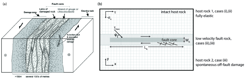
Figure 1: (a) Typical strike-slip fault zone structure showing a multiple fault core with associated damage zone in a quartzofeldspathic country rock (from [56]). (b) Sketch of the GPR model setup for 2D in-plane right-lateral shear fracture under compression used throughout Sec.33.1. In light grey we depict the prescribed fault core of length $L_{fc}$ and width $W_{fc}$ which is fully damaged ($\xi=1$) and embedded in intact host rock ($\xi=0$). The material properties and rheology of the host rock and fault core differ and are detailed in Tables S1 and S2. Grey lines illustrate the initial mesh refinement, which can dynamically adapt as detailed in Table S3.

3.1 Earthquake shear fracture across a diffuse fault zone

In the following, we explore the GPR diffuse fault zone approach extending the modeling of dynamic earthquake rupture beyond treatment as a discontinuity in the framework of elastodynamics. Fig. 1 illustrates the model setup corresponding to the geological structure of a typical strike-slip fault zone. Dynamic rupture within the ’fault core’ is governed by a friction-like behaviour achieved by time-dependent modulation of the shear relaxation time $\tau_{D}$ of the fault core’s fully damaged material. At the onset of frictional yielding, the shear relaxation time ($\tau_{D}$) decreases exponentially as in (6) with a time-dependent $\beta^{{}^{\prime}}_{D}$. The temporal evolution of $\beta^{{}^{\prime}}_{D}$ is modulated at a constant rate during rupture as $\beta^{{}^{\prime}}_{D}(t)\,=\,\beta_{D}\,\min{\left(1,\,\max{\left(0,\,1-C_{1}\,t\right)}\right)}$ where $C_{1}$ and $\beta_{D}$ are constant. Visco-elastic slip accumulates across the diffuse fault core coupled to either fully elastic wave propagation or Drucker-Prager type damage in the host rock.

i) Kinematic self-similar Kostrov-like crack. We first model a kinematically driven non-singular self-similar shear crack analog to Kostrov’s solution for a singular crack [46] to study the relation between fault slip, slip rate and shear stress in comparison to traditional approaches, while imposing tractions here avoids the full complexity of frictional rupture dynamics. The 2D setup [20, e.g.] assumes a homogeneous isotropic elastic medium (Table S2, $c_{s}=c_{p}/\sqrt{3}$), and a pre-assigned fault interface loaded by initial normal stress $\sigma_{n}=40\,\mathrm{MPa}$ and shear stress $\tau=20\,\mathrm{MPa}$. An in-plane right-lateral shear crack is driven by prescribing the (sliding) friction $\mu_{f}$ as linearly time-dependent weakening: $\mu_{f}(x,t)=\text{max}\{{f_{d}},{f_{s}}-({f_{s}}-{f_{d}})(v_{r}t-|x|)/{R_{c}}\}$, with process zone size ${R_{c}}=250\,\mathrm{m}$, rupture speed $v_{r}=2000\,\mathrm{m/s}$, static friction ${f_{s}}=0.5$ and dynamic friction ${f_{d}}=0.25$. We empirically find that choosing $C_{1}=10$ reproduces the propagating shear crack in the reference solution. Thus, $\beta^{{}^{\prime}}_{D}$ evolves linearly from $\beta_{D}$ to 0 during rupture.

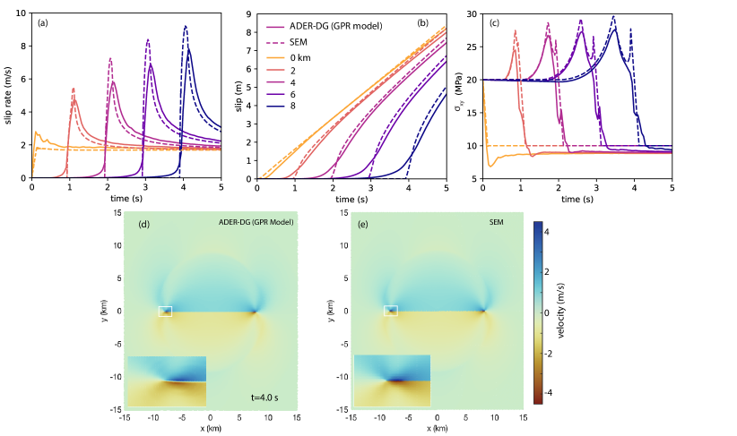
Figure 2: Comparison of the self-similar Kostrov-like crack of the diffuse GPR model (ADER-DG, $p=6$, $W_{fc}=100\,\mathrm{m}$, $L_{fc}=20\,\mathrm{km}$, fault core and host rock material are ’host rock 1’, static AMR) with the discrete fault spectral element SEM2DPACK ($p=6$, $h=100\,\mathrm{m}$) solution; (a) Slip rate, (b) slip and (c) shear stress time series at increasing hypocentral distances, (d,e) velocity wavefield at $t=4\,\mathrm{s}$ (see also Animation S1), and zoom into the rupture tip.

We assume a fully-damaged fault core ($\xi=1$) of prescribed length $L_{fc}=20\,\mathrm{km}$ and width $W_{fc}=100\,\mathrm{m}$ embedded in a continuum material resembling intact elastic rock ($\xi=0$) as illustrated in Fig. 2a. Both, the fault core and the surrounding host rock are treated as the same continuum material besides their differences in $\xi$. The GPR specific material parameters are detailed as ‘host rock 1’ (here, $\lambda_{D}=\lambda_{I},\mu_{D}=\mu_{I}$) in Table S1 in the supplementary material. The model domain is of size $70\,\mathrm{km}\times 70\,\mathrm{km}$ bounded by Dirichlet boundary conditions and employs a statically refined mesh surrounding the fault core. The domain is discretised into hierarchical Cartesian computational grids, spaced $h=2800\,\mathrm{m}$ at the coarsest level, and $h=311\,\mathrm{m}$ at the second refinement level (Table S3). We use polynomial degree $p=6$ and the subcell Finite Volume limiter counts $2\,p+1=13$ subcells in each spatial dimension. Fig.2a-c compares slip, slip rate and shear traction during diffuse crack propagation modeled with the GPR model to a spectral element solution assuming a discrete fault interface spatially discretised with $h=100\,\mathrm{m}$ with SEM2DPACK [2]. The GPR model analog captures the kinematics (i.e., stress drop and fault slip) of the self-similar singular Kostrov crack as well as the emanated seismic waves (Fig. 2d,e and Animation S1), while introducing dynamic differences on the scale of the diffuse fault (zoom-in in Fig. 2d). Slip velocity (Fig. 2a) remains limited in peak, similar to planar fault modeling with off-fault plastic deformation [30]. Fault slip (Fig. 2b) appears smeared out at its onset, yet asymptotically approaches the classical Kostrov crack solution. Similarly, shear stresses (Fig. 2c) appear limited in peak and more diffuse, specifically with respect to the secondary peak associated with the passing rupture front. Importantly, (dynamic) stress drops are comparable to the expectation from fracture mechanics for a plane shear crack (even though peak and dynamic level appear shifted). At the crack tip, we observe an initial out-of-plane rotation within the fault core leading to a localised mismatch in the hypocentral region and at the onset of slip across the fault. The GPR model approaches the analytical solution, as illustrated for increasing polynomial degree $p$ in the electronic supplement (Fig. S1).

ii) Spontaneous dynamic rupture. We next model spontaneous dynamic earthquake rupture in a 2D version [20] of the benchmark problem TPV3 [39] for elastic spontaneous rupture propagation defined by the Southern California Earthquake Center. Our setup resembles the kinematic model (Fig. 1a) including the time-dependent choice of $\beta^{{}^{\prime}}_{D}(t)$ with $C_{1}=10$ with an important distinction: we assume a low-rigidity fault core (‘low velocity fault rock’ in Table S1) by setting P-wave and S-wave velocity in the fault core 50% lower, i.e. $\lambda(\xi)$ and $\mu(\xi)$ are decreased by 30%, with respect to the intact rock. A 50% reduction of seismic wave speeds matches natural fault zone observations. The thickness of the low velocity fault rock unit equals the thickness of the fault core itself where $\xi=1$. The surrounding country rock is again parameterised as fully elastic with the ‘host rock 1’ GPR parametrisation (Table S1). The fault core is $L_{fc}=30\,\mathrm{km}$ long and $W_{fc}=100\,\mathrm{m}$ wide, the domain size is $40\,\mathrm{km}\times 40\,\mathrm{km}$, initial loading is $\sigma_{yy}=-120\,\mathrm{MPa}$ and $\sigma_{xy}=70\,\mathrm{MPa}$. The computational grid is spaced $h=1600\,\mathrm{m}$ at the coarsest level, and $h=177\,\mathrm{m}$ at the second refinement level (Table S3). Fig. 3 compares, similar to the kinematic case, the diffuse low-rigidity fault ADER-DG GPR results to an elastic discrete fault interface spectral element solution. Fault slip rates (Fig. 3a) are limited in peak and are now clearly affected by smaller scale dynamic complexity, e.g. out-of-plane crack rotation and wave reflections, within the fault core. Fault slip (Fig. 3b) asymptotically resembles the discontinuous, elastic solution. Shear stresses (Fig. 3c) are smeared out and shifted, but capture (dynamic) stress drops, similar to the kinematic model in i). We note that residual shear stress levels remain higher potentially reflecting oblique shear developing within the diffuse fault core and/or viscous behaviour within the fault core. The diffuse fault core slows down the emitted seismic waves, while amplifying sharp velocity pulses (Fig. 3d,e and Animation S2) aligning with observational findings [79]. The GPR model successfully resembles frictional linear-slip weakening behaviour[42] within the fault core by defining: $\mu_{f}(x,t)=\mathrm{max}\{{f_{d}},{f_{s}}-({f_{s}}-{f_{d}})\delta(x,t)/D_{c}\}$, with slip-weakening distance $D_{c}=0.4$ m, ${f_{s}}=0.677$ and ${f_{d}}=0.525$ similar to the discrete fault solution, $\delta(x,t)$ denotes here the diffuse slip within the fault core and is measured as the difference of displacements at its adjacent boundaries. Rupture is not initiated by an overstressed patch, which would be inconsistent with deforming material, but as a kinematically driven Kostrov-like shear-crack with $v_{r}=4000\,\mathrm{m/s}$ and within a nucleation time of $t=0.5\,\mathrm{s}$. In the diffuse model, introducing the low velocity fault rock material within the fault core is required to limit rupture speed while resembling slip rate, slip and stress evolution of the discrete reference model. We conclude that the rheological fault core properties, and not the friction law, control important crack dynamics such as rupture speed in our diffuse interface modeling, cf. [41]. A comparison of results assuming a further reduction of fault rock wave speeds to 60% is discussed in the supplementary material.

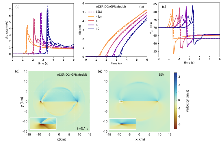
Figure 3: Computational results for the 2D TPV3 dynamic rupture problem. Comparison of the diffuse interface GPR model (ADER-DG, $p=6$, $W_{fc}=100\,\mathrm{m}$, $L_{fc}=30\,\mathrm{km}$, fault core of ’low velocity fault rock’ embedded in ’host rock 1’, static AMR) with the discrete fault spectral element SEM2DPACK solution ($p=6$, $h=100\,\mathrm{m}$), with (a) slip rate, (b) slip and (c) shear stress time series at increasing hypocentral distance. (d,e) Radiated seismic wavefield in terms of particle velocity at $t=3.1\,\mathrm{s}$ (see also Animation S2). Zoom-in the crack tips highlights dynamic rupture complexity within the low-rigidity fault core.

iii) Dynamically generated off-fault shear cracks. Localized shear banding is observed in the vicinity of natural faults spanning a wide spectrum of length scales [56], and contributes to the energy balance of earthquakes. We model dynamically generated off-fault shear cracks by combining the spontaneous dynamic rupture model embedded in ‘low velocity fault rock’ with ‘host rock 2’ outside the fault core (Table S1, $\mu_{D}=0.8571\,\mu_{I},\lambda_{D}=\lambda_{I}+0.6667\,(\mu_{I}-\mu_{D})$ in (3)). ’Host rock 2’ is governed by Drucker–Prager yielding [21, 82, 92] as given by Eq. (7), with $A=1/\sqrt{3}$, $B=\sin(\pi/18)$, and $C=-\cos(\pi/18)\cdot 95\,\mathrm{MPa}$. The model domain size is $20\,\mathrm{km}\times 15\,\mathrm{km}$ spatially discretised with $h=800\,\mathrm{m}$ at the coarsest mesh level (Table S3). We here use dynamic adaptive mesh refinement (AMR) with two refinement levels and refinement factor $\mathfrak{r}=3$ to adapt resolution in regions where the material is close to yielding. The finest spatial discretisation is $h=89\,\mathrm{m}$. Fig. 4a illustrates spontaneous shear-cracking in the extensional quadrants of the main fault core, where the passing rupture induces a dynamic bimaterial effect [84]. While previous models [82] based on ideal plasticity without damage accumulation numerically capture the formation of single sets of shear bands in Drucker-Prager type off-fault material induced by dynamic rupture propagation across a main fault, we here observe the formation of two conjugate sets of shear fractures: Cracks are distributed around two favourable orientations (Fig. 4b). Spacing and length of these shear deformation bands [52, 60] may depend on GPR material parametrization ($Y_{0},\beta_{D}$, cohesion, internal friction angle, etc., see Table S1 and [81]) as well as on the computational mesh and will motivate future analysis, as in Sec. 33.2. High particle velocity is associated with the strong growth of off-fault shear stresses near the fault tip shifting from the propagation direction of the main rupture [28]. We observe the dynamic development of interlaced conjugate shear faulting (Animation S3) resembling recent high-resolution imaging of earthquakes [76].

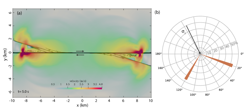
Figure 4: Off-fault shear cracks spontaneously generated in the extensional quadrants of dynamic earthquake rupture (TPV3) in the GPR model (ADER-DG,$p=6$, $W_{fc}=100\,\mathrm{m}$, $L_{fc}=20\,\mathrm{km}$, fault core of ’low velocity fault rock’ embedded in Drucker-Prager type ’host rock 2’, dynamic AMR). (a) Velocity wavefield at $t=5.0\,\mathrm{s}$ (see also Animation S3). Dark colours represent the damage variable $\xi$ illustrating the fault core initialized as fully damaged (cf. Fig. 2a) and the propagating secondary off-fault cracks. (b) Polar diagram of the statistical orientation of off-fault shear cracks. The two dominant orientations are $\approx 20^{\circ}$ and $\approx 120^{\circ}$. The maximum compressive stress ($\sigma_{1}$) has an orientation angle of $65.3^{\circ}$.

3.2 Crack formation in a rock-like disc

The GPR framework can be applied to capture tensile fracture, important for earthquake nucleation processes and the microscale of fault zone fracture and damage. We now show that our model is able to correctly describe the fracture mechanisms observed in laboratory settings. Specifically, we reproduce the experimental results of [38] which involve the compression of a rock disc along its diameter (a so-called Brazilian test). In this case the disc presents a central slit with a given orientation, which influences the early stages of the failure of the rock sample. The test is carried out in two space dimensions on a square computational domain centered at the origin and with sidelength 2.2 units. The interface of the disc is defined by setting $\alpha=0$ outside of the unit-radius circle, without requiring a boundary-fitted mesh. The material used in this test has been derived as a weakened variant of a granite-like brittle rock. In particular, it replicates the strong difference in shear resistance found under compression or tensile loads. The material is characterised by the following choice of parameters: $\rho=2620\,\mathrm{kg/m^{3}}$, $\mu_{I}=\lambda_{I}=21.44\,\mathrm{GPa}$, $\mu_{D}=\lambda_{D}=150.08\,\mathrm{MPa}$, $\theta_{0}=1$, $Y_{0}=10\,\mathrm{MPa}$, $Y_{1}=1\,\mathrm{Pa}$, $a=60$, $\tau_{{I}0}=10^{5}\,\mathrm{s}$, $\tau_{{D}0}=10^{-3}\,\mathrm{s}$, $\beta_{I}=\beta_{D}=0$. For $|y|>1$ the material is modified by setting $Y_{0}=Y_{1}=100\,\mathrm{TPa}$ to model unbreakable clamps. Thermal effects are neglected. For this test, the coefficients of the Drucker–Prager equivalent stress formula (7) are $A=1.0,\ B=1.5,$ and $C=-2.0\,\mathrm{MPa}$. In Fig. 5 we report the computational results from an ADER-DG ($p=3$) scheme on a uniform Cartesian mesh of 192 by 192 cells, showing good agreement with the experimental data. For a detailed mesh refinement study, see the supplementary material.

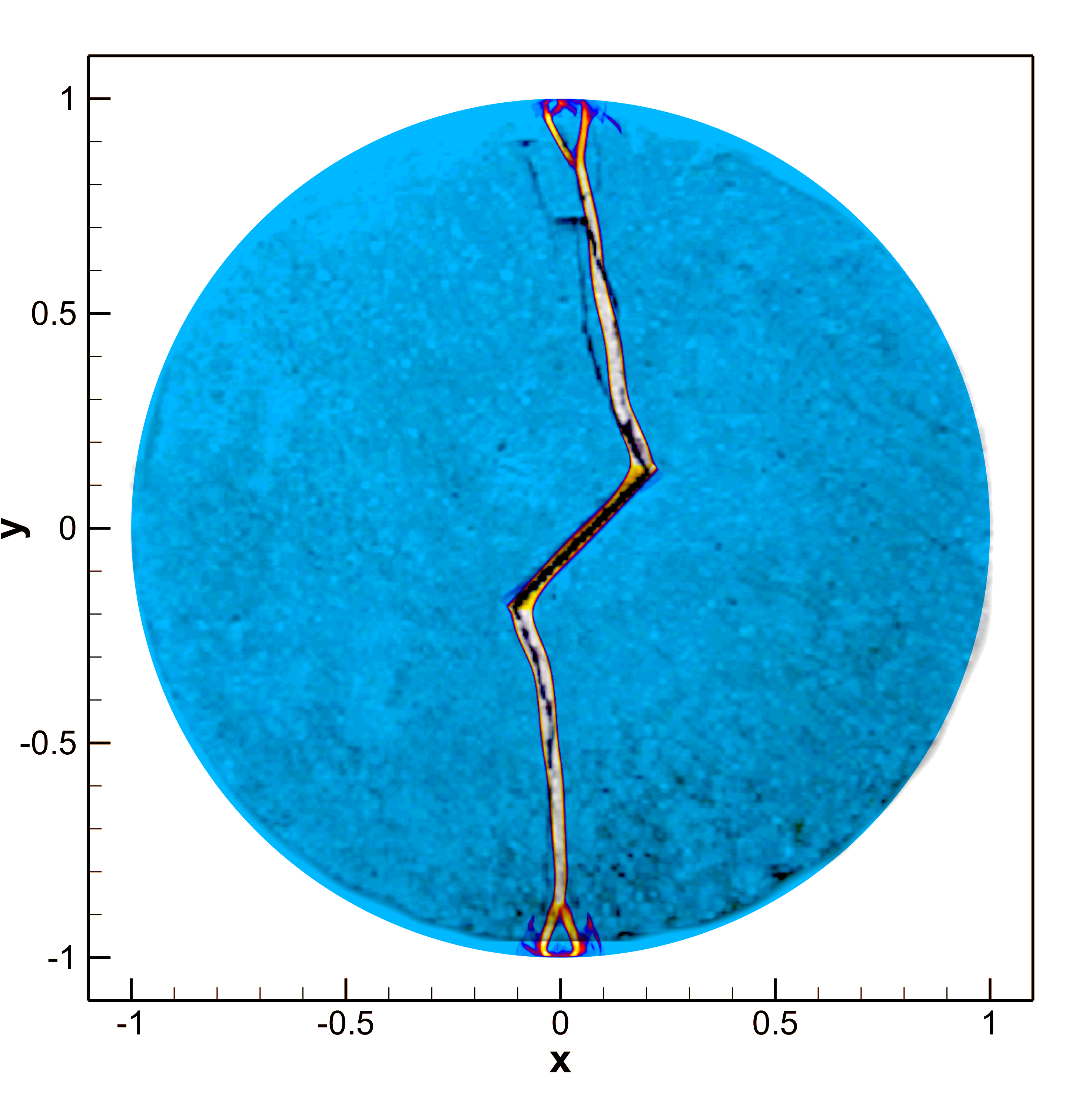
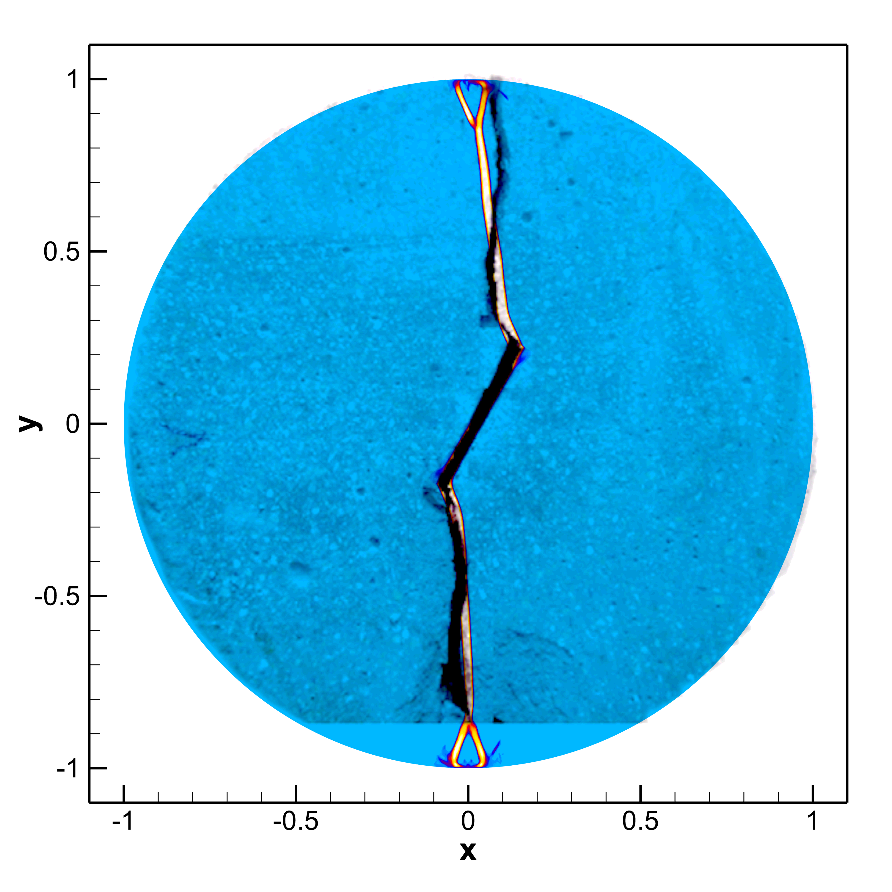
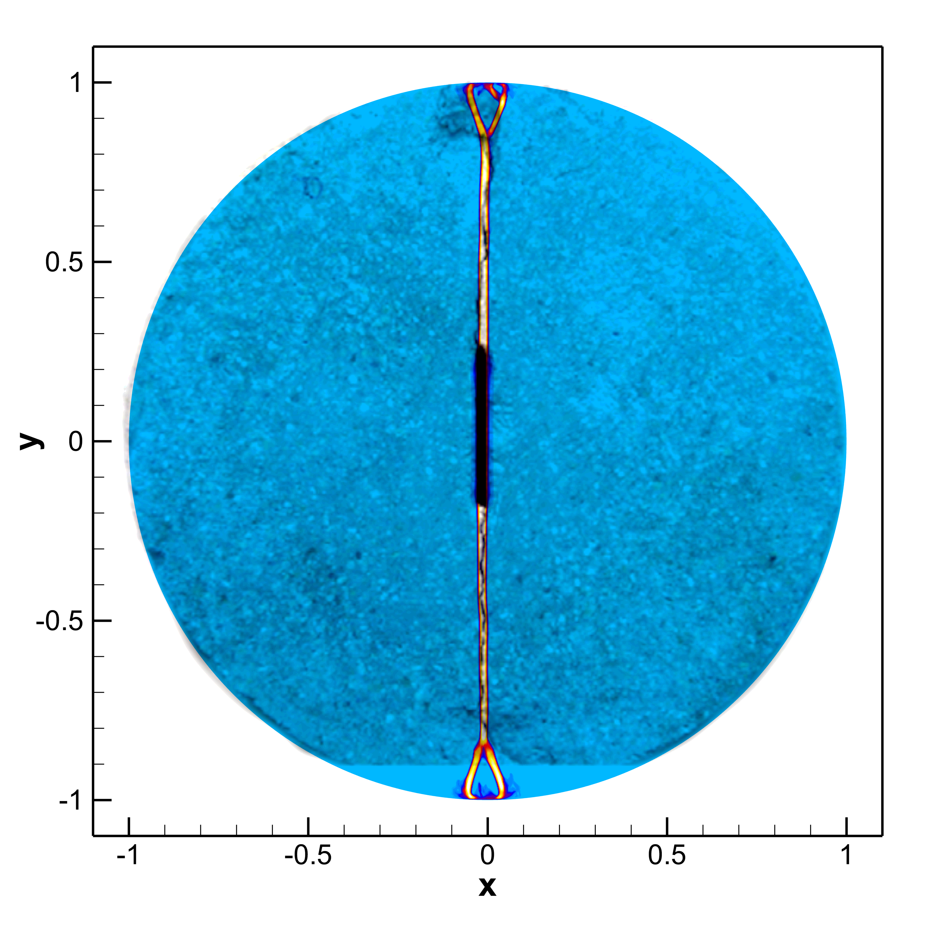
Figure 5: Crack formation in a rock-like disc under vertical load (Brazilian test) for different angles of the pre-damaged area. Comparison of the contour colors of the damage variable $\xi$ obtained in the numerical simulations of the GPR model with the cracks observed in experiments. The simulation results are overlaid on top of the photographs from [38]. From left to right: $45^{\circ}$, $60^{\circ}$ and $90^{\circ}$. Only the regions of the disc where $\alpha>0.5$ are shown.

3.3 Phase transition and natural convection in molten rock-like material

Seismic fault slip velocities and low thermal conductivity of rock can lead to the formation of veins of molten rock (pseudotachylytes), which are thought of as an unambiguous indicator of earthquake deformation, however, are not common features of active faults [77]. In our model, the phase transition between solid and liquid occurs simply via the definition of the total energy by adding the contribution of the latent heat for $T>T_{c}$, see (2), and by modifying the relaxation time for $T>T_{c}$. More precisely, in this example, the relaxation time $\tau_{1}$ is not computed according to (5) and (6) but is considered constant (time-independent) in the solid state and is computed in terms of the dynamic viscosity $\eta$ as $\tau_{1}=\frac{6\eta}{\rho_{0}c_{s}^{2}}$ for the molten state ($T>T_{c}$) treated as a Newtonian fluid. Also, in this example, $\theta_{1}$ has to be taken as $\theta_{1}=\tau_{1}c_{s}(\xi)^{2}/3|{\bm{A}}|^{-5/3}$, see the result of the asymptotic analysis presented in [23]. In the supplementary material of this paper we validate our simple approach for phase transition for a well-known benchmark problem with exact solution, namely the Stefan problem, see [5]. The obtained results clearly show that the proposed model can properly deal with heat conduction and phase transition between liquid and solid phases.

Next, we show the capability of the GPR model to describe also the motion of viscous fluids under the influence of gravity. The stresses acting on faults are key initial conditions for earthquakes and seismic fault dynamics, but are poorly known. At very long time scales, these initial conditions are governed by plate tectonics and mantle convection, which is included in the GPR model as a special case. We therefore simulate a rising bubble in molten rock-like material. In the following, we use SI units. The critical temperature is set to $T_{c}=1000$, the latent heat is $h_{c}=1000$, the gravity vector is $\mathbf{g}=(0,-9.81)$ and the dynamic viscosity of the molten material is $\eta=20$. We furthermore set the remaining parameters to $\rho_{0}=2000$, $\gamma=2$, $p_{0}=2\cdot 10^{5}$, $c_{v}=0.1$, $c_{s}=5$, $\alpha=5$ and $\lambda=0.2$. Initially we set $T=1500$, $v_{i}=0$, ${\bm{A}}={\bm{I}}$, ${\bm{J}}=0$, $p=10^{5}-\|\mathbf{g}\|\rho_{0}y$ and a hot circular bubble of radius $R=0.2$ is initially centered at $\mathbf{x}_{c}=(0,0)$ with a temperature increase of $\Delta T=200$ for $\left\|\mathbf{x}-\mathbf{x}_{c}\right\|\leq R$. The domain is $\Omega=[-2,2]\times[-1,3]$ and simulations are carried out until $t=4$ with an ADER-DG ($p=3$) scheme on a mesh of $200\times 200$ elements. For comparison, we run two simulations, one with the GPR model presented in this paper and another simulation with the compressible Navier-Stokes equations, which serves as a reference solution for the GPR model in the viscous fluid limit. The computational results are depicted in Fig. 6, where we can observe an excellent agreement. This demonstrates that the model presented in this paper is able to correctly describe also natural convection in molten material when $T>T_{c}$.

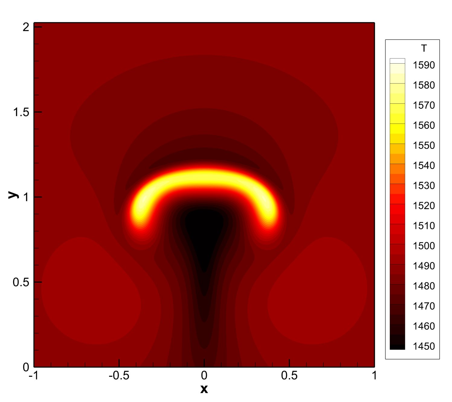
Figure 6: Temperature contours for the rising bubble problem in molten rock-like material at time $t=4$. Solution obtained with the GPR model (left) and Navier-Stokes reference solution (right). The melting temperature is set to $T_{c}=1000$.

4 Summary and Outlook

We have presented a unified hyperbolic model of inelasticity that incorporates finite strain elastoviscoplasticity and viscous fluids in a single PDE system, coupled with a hyperbolic model for continuous modeling of damage, including brittle and ductile fracture as particular cases. The governing equations are formulated in the Eulerian frame and via a diffuse interface approach permit arbitrary geometries of fractures and material boundaries without the necessity of generating interface-aligned meshes. We emphasize that the presented diffuse interface approach is not merely a way to regularize otherwise singular problems as posed by earthquake shear crack nucleation and propagation along zero-thickness interfaces, but potentially allows to fully model volumetric fault zone shearing during earthquake rupture, which includes spontaneous partition of fault slip into intensely localized shear deformation within weaker (possibly cohesionless/ultracataclastic) fault-core gouge and more distributed damage within fault rocks and foliated gouges. The model capabilities were demonstrated in several 2D examples related to rupture processes in earthquake fault zones. We compare kinematic, fully dynamic and off-fault damage GPR diffuse rupture to models employing the traditional elasto-dynamic viewpoint of a fault, namely a planar surface across which slip occurs. We show that the continuum model can reproduce and extend classical solutions, while introducing dynamic differences (i) on the scale of pre-damaged/low-rigidity fault zone, such as out-of-plane rupture rotation, limiting peak slip rates, non-frictional control of rupture speed; and (ii) on the scale of the intact host rock, such as conjugate shear cracking in tensile lobes and amplification of velocity pulses in the emitted wavefield. A natural next step is to combine the successful micro fracture laboratory scale Brazilian tests with dynamic rupture to span the entire scales of fault zone fracture. The GPR parameters for the host rock and fault zone rock material can also be calibrated to resemble natural rock, as e.g. Westerly granite [49]. Also, using the computational capabilities of the model’s ExaHyPE implementation, one can study related effects on ground shaking (see [81, 80] for GPR modeling of 3D seismic wave propagation with complex topography) and detailed 3D fault zone models [91, 86, 85, cf.] including trapped/head waves interacting with dynamic rupture [41]. Inelastic bulk processes are important during earthquake rupture [87, e.g.,], but also in between seismic events, including off-fault damage and its healing, dynamic shear localization and interseismic delocalization, and visco-elasto-plastic relaxation. Since the unified mathematical formulation proposed in this paper is able to describe elasto-plastic solids as well as viscous fluids, future work will also concern the study of fully coupled models of dynamic rupture processes triggered by mantle convection and plate tectonics. Extensions to non-Newtonian fluids will be considered, as well as to elasto-plastic saturated porous media, see e.g. the recent work presented in [43, 71]. We also plan more detailed investigations concerning the onset of melting processes in shear cracks. Finally, we note that the material failure is due to the accumulation of microscopic defects (micro-cracks in rocks or dislocations in crystalline solids). It is thus interesting to remark that the distortion field being the field of non-holonomic basis triads provides a natural basis for further development of the model towards a micro-defects-based damage theory. This can be achieved via concepts of the Riemann-Cartan geometry, such as torsion discussed in [66].

Data Accessibility.

ExaHyPE is free software hosted at www.exahype.org. The presented numerical examples will be accessible and reproducible at https://gitlab.lrz.de/exahype/ExaHyPE-Engine and https://github.com/TEAR-ERC/GPR2DR.

Funding.

This research has been supported by the European Union’s Horizon 2020 Research and Innovation Programme under the projects ExaHyPE, grant no. 671698, ChEESE, grant no. 823844 and TEAR, grant no. 852992. MD and IP also acknowledge funding from the Italian Ministry of Education, University and Research (MIUR) via the Departments of Excellence Initiative 2018–2022 attributed to DICAM of the University of Trento (grant L. 232/2016) and the PRIN 2017 project Innovative numerical methods for evolutionary partial differential equations and applications. SC was also funded by the Deutsche Forschungsgemeinschaft (DFG) under the project DROPIT, grant no. GRK 2160/1. ER was also funded within the framework of the state contract of the Sobolev Institute of Mathematics (project no. 0314-2019-0012). AG also acknowledges funding by the German Research Foundation (DFG) (grants no. GA 2465/2-1, GA 2465/3-1), by KAUST-CRG (grant no. ORS-2017-CRG6 3389.02) and by KONWIHR (project NewWave). Computing resources were provided by the Institute of Geophysics of LMU Munich [59] and the Leibniz Supercomputing Centre (project no. pr63qo).

In memoriam.

This paper is dedicated to the memory of Anne-Katrin Gabriel (*March 7, 1957 †July 25, 2020) whose creativity and curious mind will live on – in science with her daughter Alice.

Supplementary Material for:   A unified first order hyperbolic model for nonlinear dynamic rupture processes in diffuse fracture zones

1 GPR material parametrisation, geometry and computational mesh of the numerical examples of section 3(a) Earthquake shear fracture across a diffuse fault zone

material	$Y_{0}$ (Pa)	$Y_{1}$ (Pa)	$a$	$\alpha_{I}$	$\beta_{I}$	$\alpha_{D}$	$\beta_{D}$	$\mu_{{I},{D}}$	$\lambda_{{I},{D}}$
host rock 1	1.8e22	1.0e20	32.5	36.25	0.0	36.25	1.0e-6	1.0	0.0
host rock 2	1.8e8	1.0e10	32.5	36.25	0.0	36.25	1.0e-6	0.8571	0.6667
low-velocity fault rock	1.8e22	1.0e20	32.5	36.25	0.0	12.687	1.75e-7	1.0	0.0

Table S1: GPR material parameterisation for earthquake shear rupture models in section 3(a). Host rock 1 is the fully elastic material used in the full model domain of case (i), the kinematic Kostrov-like crack. The fully elastic host rock 1 is also surrounding the fault core in case (ii), the spontaneous dynamic rup-ture example. Host rock 2 is the Drucker-Prager type off-fault material of case (iii) in which off-fault shear cracks nucleate and propagate. The (visco-)elastic low-velocity fault rock material is used within the fault core in cases (ii) and (iii) and corresponds to the fully elastic host rock 1 with 50% decreased seismic velocities. Base relaxation times have been set as $\tau_{{I}0}=10^{-6}\cdot\mu_{I}$ and $\tau_{{D}0}=10^{-6}\cdot\mu_{D}$ .

case	$\rho$ (kg/m3)	$c_{p}$ (m/s)	$c_{s}$ (m/s)	$f_{s}$	$f_{d}$	$D_{c}$ or $R_{c}$ (m)	$\sigma_{yy}$ (Pa)	$\sigma_{xy}$ (Pa)
(i)	2500	4000	2309	0.4	0.2	250	-40e6	20e6
(ii)	2676	6000	3464	0.677	0.525	0.4	-120e6	70e6
(iii)	2676	6000	3464	0.677	0.525	0.4	-120e6	70e6

Table S2: Effective GPR material properties and reference friction parameters for section 3(a). Case (i) specifies the parameters of the self-similar Kostrov-like crack model. Cases (ii) and (iii) specify the parameters of the spontaneous dynamic rupture in fully elastic and Drucker-Prager type plastic material. Note that the low-velocity fault rock material of the fault core in cases (ii) and (iii) has $c_{p}$ and $c_{s}$ 50% lower than host rock 1.

case	domain length (m)	domain width (m)	fault core length $L_{fc}$ (m)	fault core width $W_{fc}$ (m)	coarsest mesh size h (m)	static refinement width (m)	mesh refinement level; factor r
(i)	70000	70000	20000	100	2800	1400	2; 3
(ii)	40000	40000	30000	100	1600	800	2; 3
(iii)	20000	15000	20000	100	800	400	2; 3

Table S3: Geometry and computational mesh used in section 3(a). The domain is discretised into hierarchical Cartesian computational grids of two mesh refinement levels and using mesh refinement factor $r=3$. In case (i) it is spaced $h=2800$ m at the coarsest level, and $h_{min}=311$ m at the second refinement level in in the vicinity of the fault core, in case (ii) $h=1600$ m and $h_{min}=177$ m, respectively, and in case (iii), which uses dynamic AMR, $h=800$ m and $h_{min}=89$ m.

2 Earthquake shear fracture animations

Supplementary Animation S1:

A map-view animation of the p=6 GPR Kostrov-like crack and seismic wave radiation model (case i) in terms of velocity is provided as supplementary material and accessible here:
https://youtu.be/CBcbLeqaB_A

Supplementary Animation S2:

A map-view animation of the p=6 GPR dynamic rupture and seismic wavefield TPV3 model (case ii) in terms of velocity is provided as supplementary material and accessible here:
https://youtu.be/wx6-m6XS8C0

Supplementary Animation S3:

A map-view animation of the p=6 GPR co-seismic off-fault shear cracks spontaneously generated in the extensional quadrants of dynamic earthquake rupture TPV3 model and seismic wavefield (case iii) in terms of velocity is provided as supplementary material and accessible here:
https://youtu.be/95oEDZBqIiE

3 P-refinement analysis for the GPR self-similar kinematic Kostrov crack model

[capbesideposition=right,top,capbesidewidth=10cm]figure[] Fault slip rate of the self-similar Kostrov-like crack (case i) modeled with the diffuse ADER-DG GPR method under varying polynomial degree p at 4 km hypocentral distance. As refer-ence the discrete fault spectral element SEM2DPACK solution is given.

4 Low-rigidity fault zone effects on spontaneous dynamic rupture (TPV3 model)

[capbesideposition=right,top,capbesidewidth=5cm]figure[] Further reduction of P- and S-wave velocity of the rheology of the ‘low-velocity fault rock’ for GPR TPV3 (case ii) results. (a,c) are taken from Fig. 3 (a,c) in the main manuscript. (b,d) illus-trate a decrease in rupture speed and increase in peak slip rate while the stress drop is equivalent. All computational results are solving the 2D TPV3 dynamic rupture problem of the diffuse interface GPR model using an ADER-DG ($p=6$, static AMR) scheme with the discrete fault spectral element SEM2DPACK solution ($p=6$, $h=100$ m), with (a,b) slip rate and (c,d) shear stress measured at increasing hypocentral distance.

5 Validation of the phase-transition via the Stefan problem and comparison with the exact solution

Here we validate this simple approach on a well-known benchmark problem with exact solution, namely the Stefan problem, see [5]. We consider the computational domain $\Omega=[0,2]\times[-0.1,+0.1]$ with periodic boundaries in $y$ direction. The model parameters are set to $\gamma=2$, $p_{0}=10^{7}$, $\rho_{0}=1000$, $\alpha=10^{4}$, $\lambda=10^{4}$, $c_{s}=0$. The initial densities are chosen as $\rho_{L}=2000$ for $x<0$ and $\rho_{R}=1000$ for $x\geq 0$. Velocity, ${\bm{J}}$ and the pressure are initially set to zero and ${\bm{A}}$ is initialized with the identity matrix. The critical temperature is chosen as $T_{c}=900$ and the latent heat is $h_{c}=10^{4}$. We now solve the GPR model until time $t=0.2$ with a fourth order ADER-DG scheme on a uniform Cartesian mesh of $400\times 4$ elements and compare our numerical results with the exact solution of the Stefan problem at constant density, see Fig. 5. The agreement is good, in particular considering the fact that in the GPR model density and pressure do not remain constant in time, as they are instead in the exact solution of the Stefan problem. The obtained results clearly show that the proposed model can properly deal with heat conduction and phase transition between liquid and solid phase

[capbesideposition=right,top,capbesidewidth=5cm]figure[] Computational results obtained with the GPR model for the Stefan problem at time $t=0.2$. Comparison with the exact solution of the original Stefan problem at constant density. The melting temperature is set to $T_{c}=900$.

6 Mesh convergence for the Brazilian disc test

Here we report the results of a mesh convergence study carried out on the Brazilian disc test. We aim to show that the main directions in which cracks develop do not depend on the mesh resolution used in the computations. The simulations are carried out with a fourth order ADER-DG scheme with MUSCL-Hancock Finite Volume subcell limiting. We would like to stress that both the intensity of material damage and the problem geometry, as well as the local material properties, are represented by means of scalar fields, so that arbitrarily complex configurations can be simulated without requiring to use any ad-hoc meshing strategies. The setup for the test problem is shown in Fig.6, where we plot the fields associated with the geometrical field $\alpha$ (which identifies the presence of solid material or of air/vacuum) and with a material- type indicator. The use of two different sets of material properties is due to the need to model a clamping apparatus that we approximate as unbreakable. Note that no feature jump coincides with a cell boundary and in general the geometry can be skewed with respect to the computational grid, or even curved.

[capbesideposition=right,top,capbesidewidth=5cm]figure[] Computational results obtained with the GPR model for the Stefan problem at time $t=0.2$. Comparison with the exact solution of the original Stefan problem at constant density. The melting temperature is set to $T_{c}=900$.

In Fig.S1 we observe that a three-fold increase in the mesh resolution (from 64 cells per space dimension, to 96, to 128, to 192) allows to achieve better sharpness and definition of the cracks, but leaves their position essentially unaltered. For the last two steps, the crack topology converges to a stable configuration also at the points of contact between the clamps and the sample, which appear to be more sensitive to grid resolution with respect to the interior of the disc. Furthermore, in no case we are able to observe any Cartesian mesh-imprinting artefacts in our solutions.

Figure S1: Mesh convergence study for crack formation in a rock-like disc under vertical load (Brazilian test). We also compare the contour colours of the damage parameter $\xi$ obtained in the numerical simulations of the GPR model with the cracks observed in experiments. From left to right, the inclination angles of the pre-damaged slit are: $45^{\circ}$, $60^{\circ}$ and $90^{\circ}$. From top to bottom, the number of grid cells in each dimension is: 64, 96, 128, and 192.

References

- [1] M. Ambati, T. Gerasimov, and L. De Lorenzis. A review on phase-field models of brittle fracture and a new fast hybrid formulation. Computational Mechanics, 55(2):383–405, 2015.
- [2] J.-P. Ampuero. SEM2DPACK, a spectral element software for 2D seismic wave propagation and earthquake source dynamics, v2.3.8, 2012. https://sourceforge.net/projects/sem2d/.
- [3] D.J. Andrews. Rupture velocity of plane strain shear cracks. Journal of Geophysical Research, 81(32):5679–5687, 1976.
- [4] D.J. Andrews. Rupture dynamics with energy loss outside the slip zone. Journal of Geophysical Research: Solid Earth, 110(B1), 2005.
- [5] H. D. Baehr and K. Stephan. Heat and Mass Transfer. Springer, 2011.
- [6] H.S Bhat, A.J. Rosakis, and C.G. Sammis. A micromechanics based constitutive model for brittle failure at high strain rates. Journal of Applied Mechanics, 79(3), 2012.
- [7] M. J. Borden, T.J.R. Hughes, C.M. Landis, and C.V. Verhoosel. A higher-order phase-field model for brittle fracture: Formulation and analysis within the isogeometric analysis framework. Computer Methods in Applied Mechanics and Engineering, 273:100–118, 2014.
- [8] B. Bourdin, G.A. Francfort, and J.J. Marigo. Numerical experiments in revisited brittle fracture. Journal of the Mechanics and Physics of Solids, 48(4):797–826, 2000.
- [9] H.J. Bungartz, M. Mehl, T. Neckel, and T. Weinzierl. The PDE framework Peano applied to fluid dynamics: An efficient implementation of a parallel multiscale fluid dynamics solver on octree-like adaptive Cartesian grids. Computational Mechanics, 46:103–114, 2010.
- [10] S. Busto, S. Chiocchetti, M. Dumbser, E. Gaburro, and I. Peshkov. High order ADER schemes for continuum mechanics. Frontiers in Physiccs, 8:32, 2020.
- [11] Y. Cheng, Z.E. Ross, and Y. Ben-Zion. Diverse volumetric faulting patterns in the San Jacinto fault zone. Journal of Geophysical Research: Solid Earth, 123(6):5068–5081, 2018.
- [12] F.M. Chester, J.P. Evans, and R.L. Biegel. Internal structure and weakening mechanisms of the San Andreas fault. Journal of Geophysical Research: Solid Earth, 98(B1):771–786, 1993.
- [13] L.R. Chiarelli et al. Comparison of high order finite element and discontinuous Galerkin methods for phase field equations: Application to structural damage. Computers & Mathematics with Applications, 74(7):1542–1564, 2017.
- [14] S. Chiocchetti and C. Müller. A Solver for Stiff Finite-Rate Relaxation in Baer-Nunziato Two-Phase Flow Models. Fluid Mechanics and its Applications, 121:31–44, 2020.
- [15] S. Chiocchetti, I. Peshkov, S. Gavrilyuk, and M. Dumbser. High order ADER schemes and GLM curl cleaning for a first order hyperbolic formulation of compressible flow with surface tension. Journal of Computational Physics, 2020.
- [16] Y. Cui et al. Physics-based seismic hazard analysis on petascale heterogeneous supercomputers. In SC ’13: Proceedings of the International Conference on High Performance Computing, Networking, Storage and Analysis, pages 1–12, 2013.
- [17] L.A. Dalguer, K. Irikura, and J.D. Riera. Simulation of tensile crack generation by three-dimensional dynamic shear rupture propagation during an earthquake. Journal of Geophysical Research: Solid Earth, 108(B3), 2003.
- [18] S.M. Day, L.A. Dalguer, N. Lapusta, and Y. Liu. Comparison of finite difference and boundary integral solutions to three-dimensional spontaneous rupture. Journal of Geophysical Research: Solid Earth, 110(B12), 2005.
- [19] R. de Borst, J.J.C. Remmers, A. Needleman, and M.A. Abellan. Discrete vs smeared crack models for concrete fracture: bridging the gap. International journal for numerical and analytical methods in geomechanics, 28(7-8):583–607, 2004.
- [20] J. de la Puente, J.-P. Ampuero, and M. Käser. Dynamic rupture modeling on unstructured meshes using a discontinuous Galerkin method. Journal of Geophysical Research: Solid Earth, 114(B10), 2009.
- [21] D.C. Drucker and W. Prager. Soil mechanics and plastic analysis or limit design. Quarterly of Applied Mathematics, 10(2):157–165, 1952.
- [22] M. Dumbser, F. Fambri, M. Tavelli, M. Bader, and T. Weinzierl. Efficient implementation of ADER discontinuous Galerkin schemes for a scalable hyperbolic PDE engine. Axioms, 7:63, 2018.
- [23] M. Dumbser, I. Peshkov, E. Romenski, and O. Zanotti. High order ADER schemes for a unified first order hyperbolic formulation of continuum mechanics: Viscous heat-conducting fluids and elastic solids. Journal of Computational Physics, 314:824–862, 2016.
- [24] M. Dumbser, O. Zanotti, R. Loubère, and S. Diot. A posteriori subcell limiting of the discontinuous Galerkin finite element method for hyperbolic conservation laws. Journal of Computational Physics, 278:47–75, 2014.
- [25] L. O. Eastgate et al. Fracture in mode I using a conserved phase-field model. Physical Review E, 65(3):1–10, 2002.
- [26] D.W. Forsyth, T. Lay, R.C. Aster, and B. Romanowicz. Grand challenges for seismology. EOS, Transactions American Geophysical Union, 90(41):361–362, 2009.
- [27] G.A. Francfort and J.-J. Marigo. Revisiting brittle fracture as an energy minimization problem. Journal of the Mechanics and Physics of Solids, 46(8):1319–1342, 1998.
- [28] L.B. Freund. Dynamic Fracture Mechanics. Cambridge University Press, 1990.
- [29] A.A. Gabriel, J.-P. Ampuero, L.A. Dalguer, and P.M. Mai. The transition of dynamic rupture styles in elastic media under velocity-weakening friction. Journal of Geophysical Research: Solid Earth, 117(B9), 2012.
- [30] A.A. Gabriel, J.-P. Ampuero, L.A. Dalguer, and P.M. Mai. Source properties of dynamic rupture pulses with off-fault plasticity. Journal of Geophysical Research: Solid Earth, 118:4117–4126, 2013.
- [31] M. Giaquinta, P.M. Mariano, G. Modica, and D. Mucci. Ground states of simple bodies that may undergo brittle fractures. Physica D: Nonlinear Phenomena, 239(15):1485–1502, 2010.
- [32] S.K. Godunov. An interesting class of quasilinear systems. Dokl. Akad. Nauk SSSR, 139(3):521–523, 1961.
- [33] S.K. Godunov. Elements of mechanics of continuous media. Nauka, 1978. (in Russian).
- [34] S.K. Godunov, T.Y. Mikhailova, and E.I. Romenskii. Systems of thermodynamically coordinated laws of conservation invariant under rotations. Siberian Mathematical Journal, 37:690–705, 1996.
- [35] S.K. Godunov and E.I. Romenski. Nonstationary equations of nonlinear elasticity theory in Eulerian coordinates. Journal of Applied Mechanics and Technical Physics, 13(6):868–884, 1972.
- [36] H. Gomez and K.G. van der Zee. Computational Phase-Field Modeling. In Encyclopedia of Computational Mechanics Second Edition, pages 1–35. John Wiley & Sons, Chichester, UK, 2017.
- [37] A.A. Griffith. The phenomena of rupture and flow in solids. Philosophical Transactions of the Royal Society of London. Series A, Containing Papers of a Mathematical or Physical Character, 221(582-593):163–198, 1921.
- [38] H. Haeri, K. Shahriar, M. Fatehi Marji, and P. Moarefvand. Experimental and numerical study of crack propagation and coalescence in pre-cracked rock-like disks. International Journal of Rock Mechanics and Mining Sciences, 67:20 – 28, 2014.
- [39] R.A. Harris et al. A suite of exercises for verifying dynamic earthquake rupture codes. Seismological Research Letters, 89(3):1146–1162, 2018.
- [40] A. Heinecke et al. Petascale high order dynamic rupture earthquake simulations on heterogeneous supercomputers. In SC’14: Proceedings of the International Conference for High Performance Computing, Networking, Storage and Analysis, pages 3–14. IEEE, 2014.
- [41] Y. Huang, J.-P. Ampuero, and D. V. Helmberger. Earthquake ruptures modulated by waves in damaged fault zones. Journal of Geophysical Research: Solid Earth, 119(4):3133–3154, 2014.
- [42] Y. Ida. Cohesive force across the tip of a longitudinal-shear crack and griffith’s specific surface energy. Journal of Geophysical Research, 77(20):3796–3805, 1972.
- [43] H. Jackson and N. Nikiforakis. A numerical scheme for non-Newtonian fluids and plastic solids under the GPR model. Journal of Computational Physics, 387:410–429, 2019.
- [44] D. Kamensky, G. Moutsanidis, and Yu. Bazilevs. Hyperbolic phase field modeling of brittle fracture: Part I - Theory and simulations. Journal of the Mechanics and Physics of Solids, 121:81–98, 2018.
- [45] M. Kikuchi. Inelastic effects on crack propagation. Journal of Physics of the Earth, 23(2):161–172, 1975.
- [46] B.V. Kostrov. Self–similar problems of propagation of shear cracks. Journal of Applied Mathematics and Mechanics, 28(5):1077–1087, 1964.
- [47] V.I. Levitas, H. Jafarzadeh, G.H. Farrahi, and M. Javanbakht. Thermodynamically consistent and scale-dependent phase field approach for crack propagation allowing for surface stresses. International Journal of Plasticity, 111:1–35, 2018.
- [48] T. Liebe and P. Steinmann. Theory and numerics of a thermodynamically consistent framework for geometrically linear gradient plasticity. International Journal for Numerical Methods in Engineering, 51(12):1437–1467, aug 2001.
- [49] D.A. Lockner. A generalized law for brittle deformation of westerly granite. Journal of Geophysical Research: Solid Earth, 103(B3):5107–5123, 1998.
- [50] E. Lorentz and A. Benallal. Gradient constitutive relations: numerical aspects and application to gradient damage. Computer Methods in Applied Mechanics and Engineering, 194(50-52):5191–5220, dec 2005.
- [51] V. Lyakhovsky, Y. Ben-Zion, and A. Agnon. A viscoelastic damage rheology and rate-and state-dependent friction. Geophysical Journal International, 161(1):179–190, 2005.
- [52] X. Ma and A. Elbanna. Strain localization in dry sheared granular materials: A compactivity-based approach. Physical Review E, 98(2):022906, 2018.
- [53] P. M. Mariano. Physical significance of the curvature varifold-based description of crack nucleation. Rend. Lincei Mat. Appl., 21:215–233, 2010.
- [54] C. Miehe, L.M. Schänzel, and H. Ulmer. Phase field modeling of fracture in multi-physics problems. Part I. Balance of crack surface and failure criteria for brittle crack propagation in thermo-elastic solids. Computer Methods in Appl. Mechanics and Engineering, 294:449–485, 2015.
- [55] H. Mirzabozorg and M. Ghaemian. Non-linear behavior of mass concrete in three-dimensional problems using a smeared crack approach. Earthquake engineering & structural dynamics, 34(3):247–269, 2005.
- [56] T.M. Mitchell and D.R. Faulkner. The nature and origin of off-fault damage surrounding strike-slip fault zones with a wide range of displacements: A field study from the atacama fault system, northern chile. Journal of Structural Geology, 31(8):802 – 816, 2009.
- [57] N. Moës, J. Dolbow, and T. Belytschko. A finite element method for crack growth without remeshing. International Journal for Numerical Methods in Engineering, 46(1):131–150, 1999.
- [58] S. Nielsen. From slow to fast faulting: recent challenges in earthquake fault mechanics. Philosophical Transactions of the Royal Society A: Mathematical, Physical and Engineering Sciences, 375(2103):20160016, 2017.
- [59] J. Oeser, H.P. Bunge, and M. Mohr. Cluster design in the Earth Sciences – Tethys. In Int. Conference on High Performance Computing and Communications, pages 31–40. Springer, 2006.
- [60] K. Okubo et al. Dynamics, radiation, and overall energy budget of earthquake rupture with coseismic off-fault damage. Journal of Geophysical Research: Solid Earth, 124:11771–11801, 2019.
- [61] K. Okubo, E. Rougier, Z. Lei, and H.S. Bhat. Modeling earthquakes with off-fault damage using the combined finite-discrete element method. Computational Particle Mechanics, 2020.
- [62] F.X. Passelègue et al. Frictional evolution, acoustic emissions activity, and off-fault damage in simulated faults sheared at seismic slip rates. Journal of Geophysical Research: Solid Earth, 121:7490–7513, 2016.
- [63] M. Pavelka, V. Klika, and M. Grmela. Multiscale Thermo-Dynamics. De Gruyter, Berlin, 2018.
- [64] I. Peshkov, M. Pavelka, E. Romenski, and M. Grmela. Continuum Mechanics and Thermodynamics in the Hamilton and the Godunov-type Formulations. Continuum Mechanics and Thermodynamics, 30:1343–1378, 2018.
- [65] I. Peshkov and E. Romenski. A hyperbolic model for viscous newtonian flows. Continuum Mechanics and Thermodynamics, 28:85–104, 2016.
- [66] I. Peshkov, E. Romenski, and M. Dumbser. Continuum mechanics with torsion. Continuum Mechanics and Thermodynamics, 31(5):1517–1541, 2019.
- [67] V. Peshkov. Second sound in helium ii. Journal of Physics (USSR), 8:381, 1944.
- [68] A. Reinarz et al. Exahype: An engine for parallel dynamically adaptive simulations of wave problems. Computer Physics Communications, 254:107251, 2020.
- [69] A. D. Resnyansky, E. I. Romensky, and N K Bourne. Constitutive modeling of fracture waves. Journal of Applied Physics, 93(3):1537–1545, 2003.
- [70] E. Romenski, D. Drikakis, and E. Toro. Conservative Models and Numerical Methods for Compressible Two-Phase Flow. Journal of Scientific Computing, 42(1):68–95, 2010.
- [71] E. Romenski, G. Reshetova, I. Peshkov, and M. Dumbser. Modeling wavefields in saturated elastic porous media based on thermodynamically compatible system theory for two-phase solid-fluid mixtures. Computers & Fluids, 206:104587, 2020.
- [72] E. Romenski, A.D. Resnyansky, and E.F. Toro. Conservative hyperbolic formulation for compressible two-phase flow with different phase pressures and temperatures. Quarterly of Applied Mathematics, 65(2):259–279, 2007.
- [73] E. I. Romenski. Dynamic three-dimensional equations of the Rakhmatulin elastic-plastic model. Journal of Applied Mechanics and Technical Physics, 20(2):229–244, 1979.
- [74] E. I. Romenski. Deformation model for brittle materials and the structure of failure waves. Journal of Applied Mechanics and Technical Physics, 48(3):437–444, 2007.
- [75] E.I. Romenski. Hyperbolic systems of thermodynamically compatible conservation laws in continuum mechanics. Mathematical and computer modelling, 28(10):115–130, 1998.
- [76] Z.E. Ross et al. Hierarchical interlocked orthogonal faulting in the 2019 ridgecrest earthquake sequence. Science, 366(6463):346–351, 2019.
- [77] R.H. Sibson. Generation of pseudotachylyte by ancient seismic faulting. Geophysical Journal International, 43(3):775–794, 1975.
- [78] R. Spatschek, E. Brener, and A. Karma. Phase field modeling of crack propagation. Philosophical Magazine, 91(1):75–95, 2011.
- [79] P. Spudich and K. B. Olsen. Fault zone amplified waves as a possible seismic hazard along the Calaveras Fault in central California. Geophysical Research Letters, 28(13):2533–2536, 2001.
- [80] M. Tavelli et al. A simple diffuse interface approach on adaptive cartesian grids for the linear elastic wave equations with complex topography. Journal of Computational Physics, 386:158–189, 2019.
- [81] M. Tavelli, E. Romenski, S. Chiocchetti, A.-A. Gabriel, and M. Dumbser. Space-time adaptive ADER discontinuous Galerkin schemes for nonlinear hyperelasticity with material failure. Journal of Computational Physics, page 109758, 2020.
- [82] E.L. Templeton and J.R. Rice. Off-fault plasticity and earthquake rupture dynamics: 1. dry materials or neglect of fluid pressure changes. Journal of Geophysical Research: Solid Earth, 113(B9), 2008.
- [83] M.Y. Thomas and H.S. Bhat. Dynamic evolution of off-fault medium during an earthquake: a micromechanics based model. Geophysical Journal International, 214(2):1267–1280, 2018.
- [84] M.Y. Thomas, H.S. Bhat, and Y. Klinger. Effect of Brittle Off-Fault Damage on Earthquake Rupture Dynamics, chapter 14, pages 255–280. American Geophysical Union, 2017.
- [85] T. Ulrich et al. Coupled, physics-based modeling reveals earthquake displacements are critical to the 2018 Palu, Sulawesi Tsunami. Pure and Applied Geophysics, 176(10):4069–4109, 2019.
- [86] T. Ulrich, A.-A. Gabriel, J.P. Ampuero, and W. Xu. Dynamic viability of the 2016 Mw 7.8 Kaikōura earthquake cascade on weak crustal faults. Nature communications, 10(1):1–16, 2019.
- [87] T. Ulrich, A.-A. Gabriel, and E.H. Madden. Stress, rigidity and sediment strength control megathrust earthquake and tsunami dynamics. EarthArXiv, 2020. submitted. https://eartharxiv.org/s9263/.
- [88] C. Uphoff et al. Extreme scale multi-physics simulations of the tsunamigenic 2004 sumatra megathrust earthquake. In Proceedings of the international conference for high performance computing, networking, storage and analysis, pages 1–16, 2017.
- [89] T. Weinzierl and M. Mehl. Peano - A traversal and storage scheme for octree-like adaptive Cartesian multiscale grids. SIAM Journal on Scientific Computing, 33:2732–2760, 2011.
- [90] C.A.J. Wibberley, G. Yielding, and G. Di Toro. Recent advances in the understanding of fault zone internal structure: a review. Geological Society, London, Special Publications, 299:5–33, 2008.
- [91] S. Wollherr, A.-A. Gabriel, and P.M. Mai. Landers 1992 ’reloaded’: Integrative dynamic earthquake rupture modeling. Journal of Geophysical Research: Solid Earth, 124(7):6666–6702, 2019.
- [92] S. Wollherr, A.-A. Gabriel, and C. Uphoff. Off-fault plasticity in three-dimensional dynamic rupture simulations using a modal Discontinuous Galerkin method on unstructured meshes. Geophysical Journal International, 214:1556–1584, 2018.
- [93] T. Yamashita. Generation of microcracks by dynamic shear rupture and its effects on rupture growth and elastic wave radiation. Geophysical Journal International, 143(2):395–406, 2000.
- [94] O. Zanotti, F. Fambri, M. Dumbser, and A. Hidalgo. Space-time adaptive ADER discontinuous Galerkin finite element schemes with a posteriori subcell finite volume limiting. Computers and Fluids, 118:204–224, 2015.
- [95] X. Zhang, S.W. Sloan, C. Vignes, and D. Sheng. A modification of the phase-field model for mixed mode crack propagation in rock-like materials. Computer Methods in Applied Mechanics and Engineering, 322:123–136, 2017.