Luminosity of radio pulsar and its new emission death line

Abstract

We investigated the pulsar radio luminosity (L), emission efficiency (ratio of radio luminosity to its spin-down power $\dot{E}$), and death line in the diagram of magnetic field ($B$) versus spin period ($P$), and found that the dependence of pulsar radio luminosity on its spin-down power ($L-\dot{E}$) is very weak, shown as $L\sim\dot{E}^{0.06}$, which deduces an equivalent inverse correlation between emission efficiency and spin-down power as $\xi\sim\dot{E}^{-0.94}$. Furthermore, we examined the distributions of radio luminosity of millisecond and normal pulsars, and found that, for the similar spin-down powers, the radio luminosity of millisecond pulsars is about one order of magnitude lower than that of the normal pulsars. The analysis of pulsar radio flux suggests that this correlations are not due to a selective effect, but are intrinsic to the pulsar radio emission physics. Their radio radiations may be dominated by the different radiation mechanisms. The cut-off phenomenon of currently observed radio pulsars in $B-P$ diagram is usually referred as the “pulsar death line”, which corresponds to $\dot{E}\approx 10^{30}$ erg$\cdot$s^-1 and is obtained by the cut-off voltage of electron acceleration gap in the polar cap model of pulsar proposed by Ruderman and Sutherland. Observationally, this death line can be inferred by the actual observed pulsar flux $S\geq$ 1 mJy and 1 kpc distance, together with the maximum radio emission efficiency of 1%. However, the observation data show that the 37 pulsars pass over the death line, including the recently observed two pulsars with long periods of 23.5 s and 12.1 s ,which violate the prediction of polar cap model. At present, the actual observed pulsar flux can reach 0.01 mJy by FAST telescope, which will arise the observational limit of spin-down power of pulsar as low as $\dot{E}\approx 10^{28}$ erg/s. This means that the new death line is downward shifted two orders of magnitude, which might be favorably referred as the “observational limit–line”, and accordingly the pulsar theoretical model for the cut-off voltage of gap should be heavily modified.

1 Introduction

It is generally accepted that the radio radiation of a pulsar originates from the generation of electron-positron pairs in its magnetic magnetosphere (Ruderman & Sutherland 1975; Sturrock 1971; Goldreich & Julian 1969; Arons & Scharlemann 1979; van den Heuvel. 2006; Machabeli & Usov 1979; Cheng & Ruderman 1980; Melrose 1978; Lin & Qiao 1997). When the radio pulsar does not have enough pairs to generate the pulses, it will be ceased (Ruderman & Sutherland 1975, hereafter RS75), which is ascribed to the limited voltage of the gap $\Phi_{max}\approx\frac{BR^{3}\Omega^{2}}{2c^{2}}$, where $B$ is the neutron star (NS) polar magnetic field strength at surface, $\Omega$ is the angular velocity associated with spin period $P$ as $\Omega=2\pi/P$, and $R$ is the NS radius. The so-called radio pulsar death line is defined by setting $\Delta V=\Phi_{max}=10^{12}{\rm Volt}\Rightarrow B_{12}/P^{2}\simeq 0.2$ (Bhattacharya & van den Heuvel 1991), where $B_{12}$ is the NS magnetic field in the units of $10^{12}$ G (Ruderman & Sutherland 1975; Bhattacharya & van den Heuvel 1991). Under the assumption of the magnetic dipole model (Shapiro & Teukolsky 1983; Lorimer & Kramer 2012; Lyne & Graham-Smith 2012), the limited voltage of the gap corresponds to the rotational energy loss rate of $\dot{E}\simeq 1.5\times 10^{30}$erg$\cdot$s^-1 (Bhattacharya & van den Heuvel 1991), which is usually referred as the death line of radio pulsars, as shown in Fig.1. Until now approximately 2700 radio pulsars have been found (ATNF Pulsar Catalogue, Manchester et al 2005; Lorimer et al 2019), most of which are situated above the death line, in the magnetic field versus period ($B-P$) diagram (see Fig. 1).

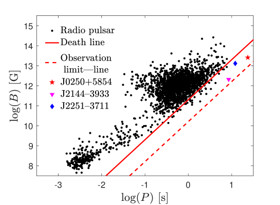
Figure 1: The magnetic field versus period ($B-P$) diagram for the radio pulsars. The solid line is the death line defined as $B_{12}/P^{2}\cong 0.2$ (e.g., Ruderman & Sutherland 1975; Bhattacharya & van den Heuvel 1991), and the dashed line is the “observational limit—line” corresponds to $\dot{E}\simeq 10^{28}$ erg s^-1 (see section 2.6). The pulsar samples are taken from the ATNF Pulsar Catalogue: https://www.atnf.csiro.au/research/pulsar/psrcat/ (Manchester et al 2005)

However, from Figure. 1, we find that 37 pulsars are observed below the death line, including the long-period pulsar J0250+5854 ($P=23.5$ s, Tan et al 2018) and J2251–3711($P=12.1$ s, Morello et al. 2019) and J2144–3933 ($P=8.5$ s, Young et al 1999). These pulsars are characterized as low spin-down power radio pulsars (hereafter low-$\dot{E}$), thus the RS75 model should be modified to explain this fact.

Zhang et al (2000) reinvestigated the radio pulsar “death lines” within the framework of the vacuum gap model (V—model) and the space—charge—limited flow model (SCLF) with either curvature radiation (CR) or inverse Compton scattering (ICS) photons as the source of pairs. They found that the ICS induced SCLF model can maintain a strong pair generation in the pulsar J2144–3933. Tan et al (2018) found that the curvature radiation and inverse Compton scattering death lines of SCLF model (Zhang et al 2000) were both located below the position of PSR J0250 + 5854. Gil & Mitra (2001) argued that the death line of curvature radiation can be moved further down by considering very curved magnetic field lines with a radius of curvature much smaller than the radius of a typical neutron star. Harding & Muslimov (2011) proposed an offset pole with a distorted magnetic field. The death line of curvature radiation in the SCLF model can move downward. Zhou et al (2017) investigated the neutron star equation of state and found that the heavier neutron stars can explain the presence of radio pulsars outside the standard death line. The most concise explanation of the current death line is proposed by Szary et al (2014). They believe that the upper limit of radio radiation efficiency ($\xi\sim 0.01$) is equivalent to the death line. Although there are many explanations at present, none of them can explain the fact that 37 radio pulsars pass through the death line.

In this paper, to pursue the cause of the death line crisis, we investigated the luminosity, radiation efficiency, and “death line” of radio pulsars. In Section 2, we introduce the calculation formula of radio luminosity and the definition of radiation efficiency. And explore whether the $\xi-\dot{E}$ association is intrinsic, where the effects of pulsar magnetic field and period on radiation efficiency are studied, and we present the “observational limit—line” to replace the death in $B-P$ diagram. Sections 3 is dedicated to the discussion and conclusion.

2 statistics of pulsar radio luminosity

In this section, we study the relation between the spin-down power and radio luminosity of pulsars.

2.1 Radio luminosity and emission efficiency

The precise estimation of the pulsar radio luminosity is difficult on account of various reasons (see Lorimer & Kramer 2012), and our analysis is based on the radio pulsar luminosities of ATNF Catalogue at the wave band of 1400 MHz (Manchester et al 2005). The observed flux density of a radio source is measured in Jansky defined as 1 Jy=$10^{-26}W\cdot m^{-2}\cdot$ Hz${}^{-1}=10^{-23}$erg$\cdot$s${}^{-1}\cdot$ cm${}^{-2}\cdot$Hz^-1, based on which the total radio luminosity ($L$) of the pulsar is calculated by the formula provided by Lorimer & Kramer (2012):

$$L=\frac{4\pi d^{2}}{\delta}sin^{2}(\frac{\rho}{2})\int_{\nu_{min}}^{\nu_{max}}S_{mean}(\nu)\,d(\nu)$$ (1)

where $d$ is the pulsar distances, the pulse duty cycle $\delta=W_{eq}/P$ with $W_{eq}$ being the equivalent pulse width. $\nu_{min}$ and $\nu_{max}$ describe the frequency range in which the pulsar is detected and studied, $S_{mean}(\nu)$ is the mean flux density measured at frequency $\nu$, and $\rho$ is the emitting angle of the pulse beam. Lorimer & Kramer (2012) employ 1400 MHz as the reference frequency and assume the typical values for all pulsars: $\delta\approx 0.04$, $\rho\approx 6^{\circ}$, $\nu_{min}\approx 10^{7}$ Hz, $\nu_{max}\approx 10^{11}$ Hz, thus the equation 1 can be expressed as follows:

$$L\simeq 7.4\times 10^{27}\,{\rm erg\cdot s^{-1}}(\frac{d}{\rm kpc})^{2}(\frac{S_{\rm 1400}}{\rm mJy})$$ (2)

where $S_{1400}$ is the mean flux density at 1400 MHz (mJy).

For the efficiency of radio pulsar radiation, defined as ratio of radio emission power to that of NS spin-down power, can be written as (e.g., Szary et al 2014; Malov & Malov 2006),

$$\xi\equiv\frac{L}{\dot{E}}$$ (3)

where $\dot{E}$ is the spin-down power (also called spin-down luminosity).

2.2 Radio luminosity and spin-down power

For radio pulsars, to uncover their emission mechanisms, we investigate the statistical properties of the radio luminosity ($L$) and emission efficiency ($\xi$) as a function of the spin-down power, respectively, as shown in Figure. 2.

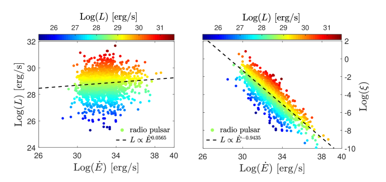
Figure 2: Dependence of the radio luminosity (left panel) and emission efficiency (right panel) on the spin-down power. The colors of samples correspond to the different values of radio luminosity. The pulsar samples are taken from the ATNF Pulsar Catalogue: https://www.atnf.csiro.au/research/pulsar/psrcat/ (Manchester et al 2005).

It is worth noting that the quantities $L$ and $\dot{E}$ of the pulsar are two independent parameters by the different measurements. The best fitting indicates that there is basically a very weak dependence between the radio luminosity and spin-down power, as $L\propto\dot{E}^{0.0565}$. The fitting coefficients of the power law index (with 95% confidence bounds) is given as 0.0565 with the regime of (0.0296,0.0834), implying that the correlation is still weak. In other words, the correlation is very diffuse and the goodness (R-square) of fit is only 0.093. In addition, the dependence of radio emission efficiency and spin-down power, $\xi-\dot{E}$, as shown in Figure. 2, is also found to be $\xi\propto\dot{E}^{-0.94}$. In fact, both correlations $L-\dot{E}$ and $\xi-\dot{E}$ are equivalent, since the difference of their power-law indices is 0.06 - 0.94 = 1. Therefore, the declaim of the inverse relation between the radio efficiency and spin-down power present no useful information of the pulsar intrinsic emission physics (Szary et al 2014), or mathematically the $\xi-\dot{E}$ correlation is equivalent to the $L-\dot{E}$ correlation. An alternative interpretation of the process underlying the cessation of pulsar emission is presented in Szary et al (2014), where a model-independent statement can be made that the death line of radio pulsars corresponds to an upper limit in the efficiency of radio emission. By the weak correlation between $L-\dot{E}$ and $\xi-\dot{E}$, we know that this interpretation of pulsar radio signal “death” is unreliable.

2.3 Radio luminosity of recycled and normal pulsars

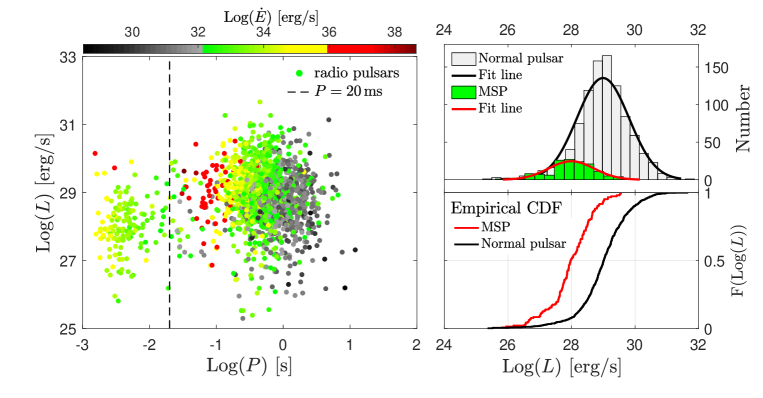
Figure 3: The left panel shows the dependence of radio luminosity on the spin period. The left panel is the histogram of radio luminosity (upper) and cumulative distribution (lower). various colors of samples correspond to the different values of pulsar spin-down power.

As can be seen from the left panel of Figure. 3, the recycled pulsars and normal pulsars can be divided into two parts by the boundary value of $P=20$ ms, and the radio luminosity of two types of pulsars have no clear correlations with the spin period. However, we also noticed that the radio luminosity of millisecond pulsars is averagely lower than that of normal pulsars. For the similar spin-down power regimes of $1.41\times 10^{32}\sim 6.25\times 10^{35}$ erg/s, the average values of both types are $3.02\times 10^{28}$ erg/s and $4.84\times 10^{29}$ erg/s, respectively, or the averaged radio luminosity of millisecond pulsars is about one order of magnitude lower than that of the normal pulsars. A further comparison of normal and millisecond pulsars is performed within the spin-down power range of $1.41\times 10^{32}\sim 6.25\times 10^{35}$ erg/s. A cumulative distribution test of their radio luminosities also exhibited the same conclusion (see CDF in Figure. 3). Through the histogram test, it was found that the radio luminosity distribution of both types of pulsars have two distinct peaks (see the histogram in Figure. 3). These clearly express the significant difference between the two types of pulsars, which may provide the valuable information for the distinctive pulsar’s radio radiation mechanism of both types of pulsars.

2.3.1 Selective effect

Cordes & Chernoff (1997) likelihood analysis on the data from extant surveys (22 pulsars with spin periods less than 20 ms) accounts for the following important selection effects: (1) the survey sensitivity described by the flux density ($S_{\rm min}$) as a function of direction, spin period, and sky coverage; (2) the interstellar scintillation, which modulates the pulse flux and causes a net increase in search volume of  30%; and (3) errors in the pulsar distance scale. It can be seen that its selection effect is mainly affected by the survey sensitivity and pulsar flux density. The detectability of pulsars by the work of Faucher-Giguère & Kaspi (2006) depends on its inherent characteristics (such as brightness, pulse period and duty cycle), its location (distance, DM, interstellar scattering and brightness temperature of the background sky) and the details of the observation system. These factors all affect the minimum observable flux density ($S_{\rm min}$). We studied the pulse flux density distribution of millisecond pulsars and normal pulsars, and then analyzed whether there is a selective effect.

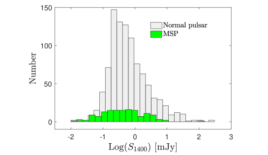
Figure 4: Histogram of flux density at 1400 MHz.

Under the condition that the energy loss rate range is $1.41\times 10^{32}\sim 6.25\times 10^{35}$ erg/s, the observed flux density is shown in Figure. 4, where the distribution range and peak value of flux density for both types of pulsars are consistent, so the selection effect is not found. Therefore, the analysis of radio flux density suggests that the upper part correlations are not due to the selection effect, but are intrinsic to the radio emission physics of pulsars.

2.3.2 emission efficiency

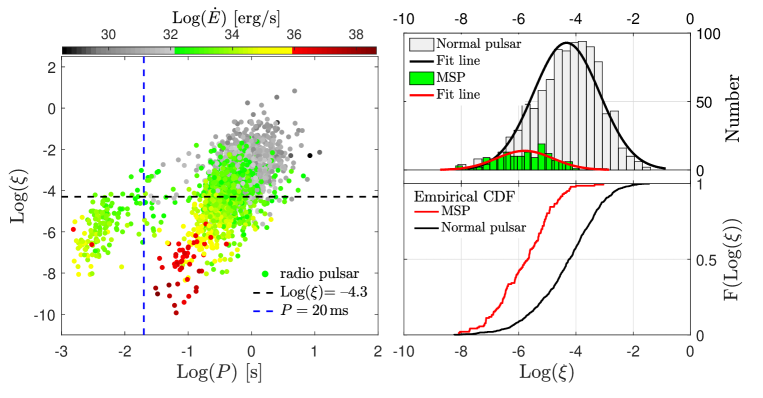
Figure 5: The left panel shows the dependence of radio emission efficiency on the spin period. The right panel is the histogram of radio emission efficiency (upper) and cumulative distribution (lower). The colors of samples correspond to the different values of pulsar spin-down power.

As can be seen from the upper panel of Figure. 5, the radio emission efficiency of the pulsar is positively correlated with the spin period (for $P>20$ms with $L\propto P^{1.9}$), which was noticed by Malov & Malov (2006). However, this conclusion has little physical significance, since the correlation $\dot{E}\propto\dot{P}/P^{3}$ will result in the proportional dependence of the efficiency $\xi$ to the spin period. We noticed that the radio emission efficiency of millisecond pulsars is generally less than $10^{-4}$ (see in Figure. 5), which is lower than those of most normal pulsars. For a similar spin-down power range $1.41\times 10^{32}\sim 6.25\times 10^{35}$ erg/s. Their average radiation efficiency is $1.73\times 10^{-5}$ and $5.69\times 10^{-4}$, respectively. Thus, it is found that the emission efficiency of millisecond pulsars is averagely one order of magnitude lower than that of normal pulsars. Examination of these two types of pulsars by histogram and cumulative distribution reveals that there exists a relatively large difference in their emission efficiency. This provides us with very valuable information because, for some physical reason, the radio luminosity of the millisecond pulsar at a similar spin-down power is one order of magnitude lower than that of a normal pulsar, and ultimately its emission efficiency is also one order of magnitude lower, which provides a valuable hint for the different radio radiation process of two types of pulsars.

2.4 radio fluxes and spin-down power relation

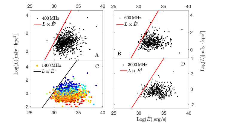
Figure 6: Dependence of the flux density on the spin-down power for various radio bands. The sub-figures A, B, C and D show the $S-\dot{E}$ relationship at center frequencies 400 MHz, 600 MHz, 1400 MHz, and 3000 MHz, respectively. The color of the sample in the sub-figure C corresponds to the date of pulsar discovery.

We investigate the statistical properties of the radio mean flux density as a function of the spin-down power as shown in Figure. 6. There is basically a very weak dependence between the two quantities. When the spin-down power of the pulsar is reduced to $\sim\dot{E}\simeq 10^{34}$ erg/s. We notice that the maximum flux density of pulsars increase with the spin-down power. The impact of energy loss rate on the pulsar flux density exist significantly. We found that there exists a proportional relation $S\propto\dot{E^{1}}$ between the flux density and spin-down power, which is clear when the spin-down power is less than $\dot{E}\simeq 10^{34}$ erg/s. This provides us with very interesting and valuable information on radio radiation mechanism. Furthermore, the relation between the flux density and spin-down power has no significant cut-off near $\dot{E}\simeq 10^{30}$ erg/s. In addition, it is worth noting that the value of the flux density has a significant stratification in the date of pulsar discovery, or more recently discovered pulsars are shown with the low flux density (see in Figure. 6 at frequencies 1400 MHz ).

2.5 Pulsar distance

There are 37 low-$\dot{E}$ pulsars, which are distributed below the death-line ($\dot{E}\simeq 10^{30}$ erg/s) in $B-P$ diagram (see Figure. 1). To investigate their properties, we compare their distances to our solar system with the other pulsars that are distributed above the death-line. In the Figure. 7, we find that the distances of the low-$\dot{E}$ pulsars are relatively close to our solar system, compared to those of other pulsars. For two groups of pulsars, below/above the death-line that are corresponding to low/high $\dot{E}$, we study their distance distributions by Kolmogorov-Smirnov test (hereafter KS-test), and obtain that the returned value of h = 1 rejects the null hypothesis at the default 5% significance level, implying the two groups belong to the different distributions. In detail, the average distance of the low (high) $\dot{E}$ pulsars is 3.6 kpc (5.6 kpc).

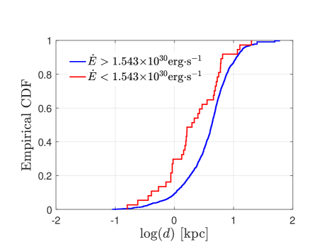
Figure 7: The cumulative distribution of pulsar distance. The red line belongs to the low-$\dot{E}$ radio pulsar, and the purple line is the other radio pulsar.

2.6 Death line and “observation limit-line”

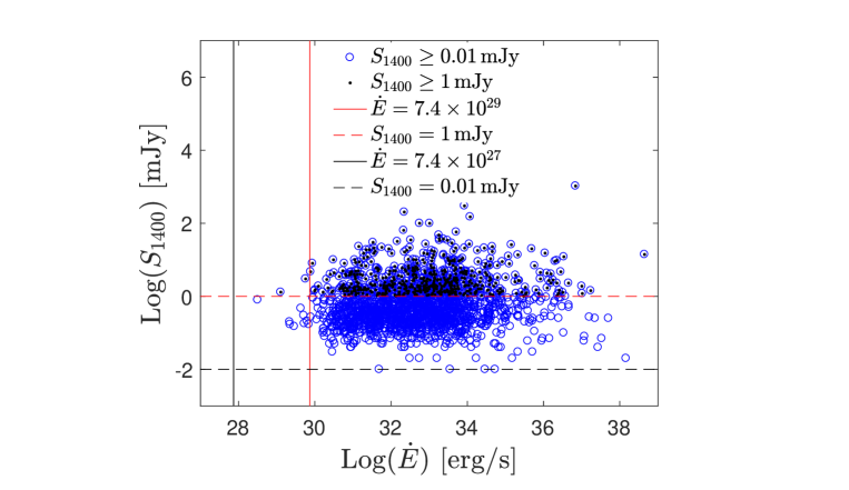
Figure 8: Dependence of the flux density on the spin-down power.

Considering equation 2 and equation 3, we can get a formula of the radio efficiency,

$$\xi\equiv\frac{L}{\dot{E}}\simeq\frac{7.4\times 10^{27}\,{\rm erg\cdot s^{-1}}(\frac{d}{\rm kpc})^{2}(\frac{S_{\rm 1400}}{\rm mJy})}{\dot{E}}\;.$$ (4)

Under the condition that the pulsar distance is 1 kpc and the observed pulsar flux density can reach $\geq$ 1 mJy, the corresponding radio luminosity of $L\geq 7.4\times 10^{27}$ erg$\cdot$s^-1 is obtained (Lorimer & Kramer 2012). If the upper limit of pulsar radiation efficiency (equation 3) is set as $\xi=$ 0.01 (proposed by Szary et al 2014), then the corresponding spin-down power $\dot{E}\geq 7.4\times 10^{29}\approx 10^{30}$ erg$\cdot$s^-1 can be derived (see in Figure 8). This means that the minimum spin-down power that can be observed under this condition is $\approx 10^{30}$ erg/s. This value is very close to the spin-down power of the death line as $1.542\times 10^{30}$ erg/s (Ruderman & Sutherland 1975). At present, especially in the observation of FAST (Nan et al. 2011), the actual observed pulsar flux is about $\geq 0.01$ mJy (Manchester et al 2005), which is corresponding to a radio luminosity of $L\geq 10^{26}$ erg$\cdot$s^-1 at the distance of 1 kpc. Therefore, the current “observation limit—line” can reach the order of $\dot{E}=10^{28}$ erg$\cdot$s^-1 (see in Figure. 1 and Figure. 8). As shown in Figure. 1, it is obvious that all currently observed radio pulsars are above this limit line, and as a result the conception of pulsar graveyard (Bhattacharya & van den Heuvel 1991) is only that is beyond “observation limit—line” of the radio telescope. This observation limitation will lead to the phenomenon that the cutoff line of “seeing”” pulsars happens at a certain spin-down power value (see Figure. 1).

From the model construction, the researchers predict the death line of pulsar that is corresponding to the cut-off of the polar cap for radio pulse emissions, however 37 low-$\dot{E}$ pulsars break this condition. On the existence of the death line, we suspect its reality, on which the following arguments are proposed.

At first, from the $L-\dot{E}$ dependence, the pulsar luminosity is very weak dependent of $\dot{E}$, this means that the low-$\dot{E}$ does not means a low radio luminosity.

Secondly, the 37 low-$\dot{E}$ pulsars are located very close to the solar system, which should account for their radio flux density over the telescope sensitivity.

Thirdly, from the flux density versus $\dot{E}$ diagram, there does not exist a sharp cut-off line to distinguish the low-$\dot{E}$ from the other sources, but the low-$\dot{E}$ pulsars are randomly distributed. From Figure. 6, the maximum flux density of pulsars increase with the $\dot{E}$, so the low-$\dot{E}$ pulsars require the high sensitivity.

Fourth, the minimum observable spin-down power is related to the minimum value of the actual flux density currently observed.

Therefore, we think that it is the telescope sensitivity not the $\dot{E}$ to account for the less pulsars appearing below the “death line”, so enhancing the telescope sensitivity could increase the number of pulsars there. How the radio radiation of pulsars died is not clear, but we found that the classic death line (RS75) and the current pulsar’s cut-off line can be ascribed to the ”observation limit–line”. Thus, we rather insist that there exists a temporary “observation limit–line”, which would be shifted to the low-$\dot{E}$ with enhancing the radio telescope sensitivity.

3 Discussion and conclusion

We investigate the statistical properties of radio luminosity of large samples of pulsars, the following conclusions are drawn below.

(1) An alternative interpretation of the process underlying the cessation of pulsar emission is not reliable. Because mathematically, the efficiency and spin-down power $\xi-\dot{E}$ correlation is equivalent to the $L-\dot{E}$ correlation, thus the inverse relation of $\xi-\dot{E}$ has the same meaning of the weak dependence of $L-\dot{E}$.

(2) For the same range of $\dot{E}$ ($1.41\times 10^{32}\sim 6.25\times 10^{35}$ erg/s), on the radio luminosity of milliseconds and normal pulsars, we find that the average value of the latter is one order of magnitude higher than the average value of the former. Their radio radiation is may dominated by different radiation mechanisms. The analysis of radio fluxes suggests that this correlations are not due to a selection effect, but are intrinsic to the pulsar radio emission physics.

(3) The maximum flux density of pulsars increase with the $\dot{E}$, shown as $S\propto\dot{E^{1}}$.. This relation is evident when the spin-down power is less than $10^{34}$ erg/s.

(4) From the RS75 model for the radio pulsar emission, there exists a death-line in $B-P$ diagram as inferred from the cut-off voltage of pulse emissions, which is corresponding to $\dot{E}\approx 10^{30}$ erg/s. From the pulsar observation, when the actual observed pulsar flux density $S\geq$ 1 mJy and distance of 1 kpc arises a radio luminosity of $L\geq 10^{28}$ erg/s, which can deduce a limit $\dot{E}\approx 10^{30}$ erg/s if the radio emission efficiency is 1%. At present, the actual observed pulsar flux density can reach a low value of 0.01 mJy, and the current observation limit line is obtained as $\dot{E}\approx 10^{28}$ erg$\cdot$s^-1 for the distance of 1 kpc and maximum radio efficiency of 1%, based on which all observed pulsars in $B-P$ diagram lie above this “new death-line”. In other words, because of this limit line, with the enhance of the telescope sensitivity, pulsars with the spin-down power less than the limited value $\dot{E}\approx 10^{28}$ erg$\cdot$s^-1 can be observed (c.f. the cases of pulsars with the long spin periods of P=8.5s and P=23.5 s). Furthermore, the conception of the current death line should be heavily modified, so does the proposed pulsar emission mechanism by RS model.

Thus, the coincidence of theoretical minimum $\dot{E}\approx 10^{30}$ erg/s with the assumed minimum observational luminosity strengthens the existence of death line. However, the 37 pulsars are found to violate the condition of pulsar death, including the three longest period pulsar (J0250+5854, J2144–3933, and J2251–3711), investigations of which indicates that most of the 37 pulsars are detected with the lower sensitivity than 1 mJy, and with the averaged distance less than those above the death line. The low spin-down powers are corresponding to the long-period pulsars, however, the observations of which exist the selective effect. As declaimed, due to the radio interference, hardware and software high-pass filters, the radio pulsar surveys typically reduce the sensitivity to the long-period pulsars (Faucher-Giguère & Kaspi 2006), and the presence of red noise also reduces the sensitivity detecting the long-period pulsars (Tan et al 2018). In addition, most pulsar surveys last a relatively short time of only a few minutes, which make most of long-period pulsars missed if there are few pulses during the observations (Tan et al 2018). With the improvement of the detection efficiency for the long-period pulsars, the more pulsar samples will appear in the region of low-$\dot{E}$ in $B-P$ diagram.

4 Acknowledgements

This research is Supported by National Natural Science Foundation of China (U1731238, 1731218, 11565010),The Science and Technology Fund of Guizhou Province ((2015)4015,(2016)-4008,(2017)5726-37), the National Natural Science Foundation of China NSFC (11773005, U1631236, U1938117. 11703001, 11690024, 11725313 ), NAOC-Y834081V01, the National Program on Key Research and Development Project (Grant No.2017YFA0402600), the Strategic Priority Research Program of the Chinese Academy of Sciences (Grant No.XDB23000000), and the CAS International Partnership Program (No.114A11KYSB20160008). We thank R.N. Manchester, G. Hobbs and D. Lorimer for discussions. We are also grateful for the anonymous referee for critic comments that help us to improve the quality of the paper. )

References

- Arons & Scharlemann (1979) Arons, J., & Scharlemann, E. T. 1979, ApJ, 231, 854
- Bhattacharya & van den Heuvel (1991) Bhattacharya, D., & van den Heuvel, E. P. J. 1991, Phys. Rep., 203, 1
- Cheng & Ruderman (1980) Cheng, A. F., & Ruderman, M. A. 1980, ApJ, 235, 576
- Cordes & Chernoff (1997) Cordes J. M., Chernoff D. F., 1997, ApJ, 482, 971
- Faucher-Giguère & Kaspi (2006) Faucher-Giguère, C.-A., & Kaspi, V. M. 2006, ApJ, 643, 332
- Gil & Mitra (2001) Gil, J., & Mitra, D. 2001, ApJ, 550, 383
- Goldreich & Julian (1969) Goldreich, P., & Julian, W. H. 1969, ApJ, 157, 869
- Harding & Muslimov (2011) Harding, A. K., & Muslimov, A. G. 2011, ApJ, 726, L10
- Lin & Qiao (1997) Lin, W. P., Zhang, B., & Qiao, G. J. 1997, Annual Review of Earth and Planetary Sciences, 1,
- Lorimer & Kramer (2012) Lorimer, D. R., & Kramer, M. 2012, Handbook of Pulsar Astronomy, by D. R. Lorimer , M. Kramer, Cambridge, UK: Cambridge University Press, 2012,
- Lorimer et al (2019) Lorimer, D., Pol, N., Rajwade, K., et al. 2019, BAAS, 51, 261
- Lyne & Graham-Smith (2012) Lyne, A., & Graham-Smith, F. 2012, Pulsar Astronomy, by Andrew Lyne , Francis Graham-Smith, Cambridge, UK: Cambridge University Press, 2012,
- Manchester et al (2005) Manchester, R. N., Hobbs, G. B., Teoh, A., & Hobbs, M. 2005, AJ, 129, 1993
- Machabeli & Usov (1979) Machabeli, G. Z., & Usov, V. V. 1979, NASA STI/Recon Technical Report N, 80,
- Melrose (1978) Melrose, D. B. 1978, ApJ, 225, 557
- Malov & Malov (2006) Malov, I. F., & Malov, O. I. 2006, Astronomy Reports, 50, 483
- Morello et al. (2019) Morello, V., Keane, E. F., Enoto, T., et al. 2019, arXiv:1910.04124
- Nan et al. (2011) Nan, R., Li, D., Jin, C., et al. 2011, International Journal of Modern Physics D, 20, 989
- Ruderman & Sutherland (1975) Ruderman, M. A., & Sutherland, P. G. 1975, ApJ, 196, 51
- Shapiro & Teukolsky (1983) Shapiro, S. L., & Teukolsky, S. A. 1983, Research supported by the National Science Foundation. New York, Wiley-Interscience, 1983, 663 p.,
- Szary et al (2014) Szary, A., Zhang, B., Melikidze, G. I., Gil, J., & Xu, R.-X. 2014, ApJ, 784, 59
- Sturrock (1971) Sturrock, P. A. 1971, ApJ, 164, 529 187
- Tan et al (2018) Tan, C. M., Bassa, C. G., Cooper, S., et al. 2018, ApJ, 866, 54
- van den Heuvel. (2006) van den Heuvel, E P J. Science, 2006, 312: 539
- Young et al (1999) Young, M. D., Manchester, R. N., & Johnston, S. 1999, Nature, 400, 848
- Zhang et al (2000) Zhang, B., Harding, A. K., & Muslimov, A. G. 2000, ApJ, 531, L135
- Zhou et al (2017) Zhou, X., Tong, H., Zhu, C., & Wang, N. 2017, MNRAS, 472, 2403